11institutetext: Ethan Anderes 22institutetext: Department of Statistics, University of California Davis, California, U.S.A. 22email: anderes@ucdavis.edu 33institutetext: Steffen Borgwardt (corresponding author) 44institutetext: Fakultät für Mathematik, Technische Universität München, Germany 44email: borgwardt@ma.tum.de 55institutetext: Jacob Miller 66institutetext: Department of Mathematics, University of California Davis, California, U.S.A. 66email: jmiller@math.ucdavis.edu

Discrete Wasserstein Barycenters:
Optimal Transport for Discrete Data

Ethan Anderes    Steffen Borgwardt    Jacob Miller
Abstract

Wasserstein barycenters correspond to optimal solutions of transportation problems for several marginals, and as such have a wide range of applications ranging from economics to statistics and computer science. When the marginal probability measures are absolutely continuous (or vanish on small sets) the theory of Wasserstein barycenters is well-developed (see the seminal paper ac-11 ). However, exact continuous computation of Wasserstein barycenters in this setting is tractable in only a small number of specialized cases. Moreover, in many applications data is given as a set of probability measures with finite support. In this paper, we develop theoretical results for Wasserstein barycenters in this discrete setting. Our results rely heavily on polyhedral theory which is possible due to the discrete structure of the marginals.

Our results closely mirror those in the continuous case with a few exceptions. In this discrete setting we establish that Wasserstein barycenters must also be discrete measures and there is always a barycenter which is provably sparse. Moreover, for each Wasserstein barycenter there exists a non-mass-splitting optimal transport to each of the discrete marginals. Such non-mass-splitting transports do not generally exist between two discrete measures unless special mass balance conditions hold. This makes Wasserstein barycenters in this discrete setting special in this regard.

We illustrate the results of our discrete barycenter theory with a proof-of-concept computation for a hypothetical transportation problem with multiple marginals: distributing a fixed set of goods when the demand can take on different distributional shapes characterized by the discrete marginal distributions. A Wasserstein barycenter, in this case, represents an optimal distribution of inventory facilities which minimize the squared distance/transportation cost totaled over all demands.

Keywords:
barycenter optimal transport multiple marginals polyhedral theory mathematical programming
MSC:
90B80 90C05 90C10 90C46 90C90

1 Introduction

Optimal transportation problems with multiple marginals are becoming important in applications ranging from economics and finance bhp-13 ; ce-10 ; cmn-10 ; ght-14 to condensed matter physics and image processing bpg-12 ; cfk-13 ; jzd-98 ; rpdb-12 ; ty-05 . The so-called Wasserstein barycenter corresponds to optimal solutions for these problems, and as such has seen a flurry of recent activity (see ac-11 ; bk-12 ; bll-11 ; coo-14 ; cd-14 ; mmh-11 ; mtbmmh-15 ; p-11b ; p-13 ; p-11 ; p-14 ; tmmh-14 ). Given probability measures P1,,PNsubscript𝑃1subscript𝑃𝑁P_{1},\ldots,P_{N} on dsuperscript𝑑\mathbb{R}^{d}, a Wasserstein barycenter is any probability measure P¯¯𝑃\bar{P} on dsuperscript𝑑\mathbb{R}^{d} which satisfies

i=1NW2(P¯,Pi)2=infP𝒫2(d)i=1NW2(P,Pi)2superscriptsubscript𝑖1𝑁subscript𝑊2superscript¯𝑃subscript𝑃𝑖2subscriptinfimum𝑃superscript𝒫2superscript𝑑superscriptsubscript𝑖1𝑁subscript𝑊2superscript𝑃subscript𝑃𝑖2\sum_{i=1}^{N}W_{2}(\bar{P},P_{i})^{2}=\inf_{P\in\mathcal{P}^{2}(\mathbb{R}^{d})}\sum_{i=1}^{N}W_{2}(P,P_{i})^{2} (1)

where W2subscript𝑊2W_{2} denotes the quadratic Wasserstein distance and 𝒫2(d)superscript𝒫2superscript𝑑\mathcal{P}^{2}(\mathbb{R}^{d}) denotes the set of all probability measures on dsuperscript𝑑\mathbb{R}^{d} with finite second moments. See the excellent monographs v-03 ; v-09 for a review of the Wasserstein metric and optimal transportation problems.

Much of the recent activity surrounding Wasserstein barycenters stems, in part, from the seminal paper ac-11 . In that paper, Agueh and Carlier establish existence, uniqueness and an optimal transport characterization of P¯¯𝑃\bar{P} when P1,,PNsubscript𝑃1subscript𝑃𝑁P_{1},\ldots,P_{N} have sufficient regularity (those which vanish on small sets or which have a density with respect to Lebesgue measure). The transportation characterization of P¯¯𝑃\bar{P}, in particular, provides a theoretical connection with the solution of (1) and the estimation of deformable templates used in medical imaging and computer vision (see jzd-98 ; ty-05 and references therein). Heuristically, any measure P¯¯𝑃\bar{P} is said to be a deformable template if there exists a set of deformations φ1,,φNsubscript𝜑1subscript𝜑𝑁\varphi_{1},\ldots,\varphi_{N} which push-forward P¯¯𝑃\bar{P} to P1,,PNsubscript𝑃1subscript𝑃𝑁P_{1},\ldots,P_{N}, respectively, and are all “as close as possible” to the identity map. Using a quadratic norm on the distance of each map φ1(x),,φN(x)subscript𝜑1𝑥subscript𝜑𝑁𝑥\varphi_{1}(x),\ldots,\varphi_{N}(x) to x𝑥x, a deformable template P¯¯𝑃\bar{P} then satisfies

P¯arginfP𝒫2(d)[inf {(φ1,,φN) s.t. s.t. φi(P)=Pi} i=1Nd|φi(x)x|2𝑑P(x)].¯𝑃argsubscriptinfimum𝑃superscript𝒫2superscript𝑑delimited-[]subscriptinfimum {(φ1,,φN) s.t. s.t. φi(P)=Pi} superscriptsubscript𝑖1𝑁subscriptsuperscript𝑑superscriptsubscript𝜑𝑖𝑥𝑥2differential-d𝑃𝑥\bar{P}\in\text{arg}\inf_{P\in\mathcal{P}^{2}(\mathbb{R}^{d})}\left[\inf_{\shortstack{\scriptsize$\{(\varphi_{1},\ldots,\varphi_{N})$\phantom{ s.t. }\\ \scriptsize s.t. $\varphi_{i}(P)=P_{i}\}$ }}\sum_{i=1}^{N}\int_{\mathbb{R}^{d}}|\varphi_{i}(x)-x|^{2}dP(x)\right]. (2)

The results of Agueh and Carlier establish that (1) and (2) share the same solution set when P1,,PNsubscript𝑃1subscript𝑃𝑁P_{1},\ldots,P_{N} have densities with respect to Lebesgue measures (for example).
Refer to caption
Refer to caption
Refer to caption
Refer to caption
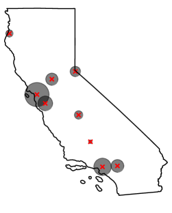
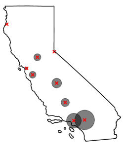
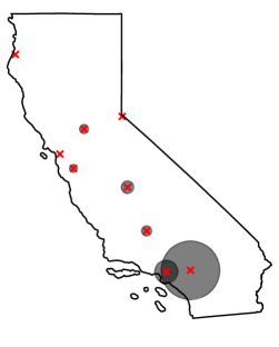
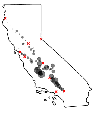
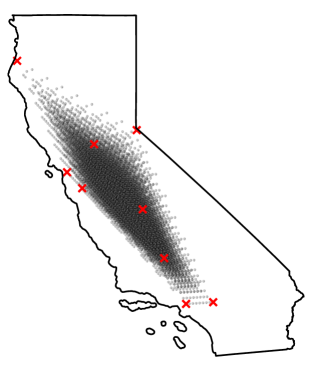
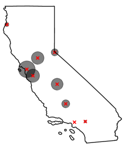
Figure 1: The above four images represent hypothetical monthly demands (as a percentage of total supply) for distributing a fixed set of goods to nine California cities (denoted by red ‘x’ marks) in four different months (February, March, June and July). Percent demand within each month is plotted proportional to disk area and is computed from monthly average temperature and population within each city (see Section 4 for details). When percent demand is treated as a discrete probability distribution, one for each month, the Wasserstein barycenter represents the optimal distribution of inventory facilities which minimize total squared distance/transportation cost over multiple monthly demand requirements. This example serves to illustrate the applicability of the main theoretical properties derived in this paper. Theorem 2.2, for example, establishes that the optimal inventory distribution is a sparse discrete probability distribution with tight bounds on the scarcity of the barycenter support. In particular, the optimal inventory facilities are located at a small number of sites with relatively large storage capacity, rather than a large number small-capacity facilities distributed over a diffuse set of locations. Theorem 2.1 shows that the optimal transportation plan assigns each to barycenter inventory facility exactly one city to supply each month. Indeed, this type of non-mass-splitting property of optimal mass transportation is known for absolutely continuous probability distributions but does not usually hold for discrete probability distributions. The discrete Wasserstein barycenter is unique in this regard: there always exists a non-mass-splitting optimal transportation plan to each of the individual probability distributions (represented by monthly demand in this example). The Wasserstein barycenter for this example is shown in Figure 2 and some of the optimal transportation plans are shown in Figure 3. Finally, the computational details of this example are presented in Section 4.

While absolutely continuous barycenters are mathematically interesting, in practice, data is often given as a set of discrete probability measures P1,,PNsubscript𝑃1subscript𝑃𝑁P_{1},\ldots,P_{N}, i.e. those with finite support in dsuperscript𝑑\mathbb{R}^{d}. For example, in Figure 1 the discrete measures denote different demand distributions over 999 California cities for different months (this example is analyzed in detail in Section 4). For the remainder of the paper we refer to a discrete Wasserstein barycenter as any probability measure P¯¯𝑃\bar{P} which satisfies (1) and where all the P1,,PNsubscript𝑃1subscript𝑃𝑁P_{1},\ldots,P_{N} have discrete support.

In this paper we develop theoretical results for discrete Wasserstein barycenters. Our results closely mirror those in the continuous case with a few exceptions. In the discrete case, the uniqueness and absolute continuity of the barycenter is lost. More importantly, however, is the fact that P¯¯𝑃\bar{P} is provably discrete when the marginals are discrete (see Proposition 1). This guarantees that finite-dimensional linear programming will yield all possible optimal P¯¯𝑃\bar{P}, and this in turn is utilized in this paper to study the properties of these barycenters from the point of view of polyhedral theory. In doing so, we find remarkable differences and similarities between continuous and discrete barycenters. In particular, unlike the continuous case, there is always a discrete barycenter with provably sparse finite support; however, analogously to the continuous case, there still exists non-mass-splitting optimal transports from the discrete barycenter to each discrete marginal. Such non-mass-splitting transports generally do not exist between two discrete measures unless special mass balance conditions hold. This makes discrete barycenters special in this regard.

In Section 2, we introduce the necessary formal notation and state our main results. The corresponding proofs are found in Section 333. To illustrate our theoretical results we provide a computational example, dicussed in Section 4 and Figures 1-3, for a hypothetical transportation problem with multiple marginals: distributing a fixed set of goods when the demand can take on different distributional shapes characterized by P1,,PNsubscript𝑃1subscript𝑃𝑁P_{1},\ldots,P_{N}. A Wasserstein barycenter, in this case, represents an optimal distribution of inventory facilities which minimize the squared distance/transportation cost totaled over all demands P1,,PNsubscript𝑃1subscript𝑃𝑁P_{1},\ldots,P_{N}.

Refer to caption
Refer to caption
Figure 2: The leftmost image shows a Wasserstein barycenter computed from 888 discrete probability distributions, each representing a different monthly demand (444 of the months are shown in Figure 1). Notice that barycenter support is extremely sparse—supported on 636363 discrete locations—as compared to the 128701287012870 possible barycenter support points (shown in the rightmost image) guaranteed by Proposition 1. Notice that Theorem 2.2 gives an upper bound of 656565 support points for the optimal Wasserstein barycenter shown here. The role of Proposition 1, on the other hand, is to give a finite set inclusion bound on the possible barycenter support points (shown at right in this example). This result yields the finite dimensional linear program characterization of optimal Wasserstein barycenters which is key to the analysis presented in this paper.

2 Results

For the remainder of this paper P1,,PNsubscript𝑃1subscript𝑃𝑁P_{1},\ldots,P_{N} will denote discrete probability measures on dsuperscript𝑑\mathbb{R}^{d} with finite second moments. Let 𝒫2(d)superscript𝒫2superscript𝑑\mathcal{P}^{2}(\mathbb{R}^{d}) denote the space of all probability measures with finite second moments on dsuperscript𝑑\mathbb{R}^{d}. Recall, a Wasserstein barycenter P¯¯𝑃\bar{P} is an optimizer to the problem

infP𝒫2(d)i=1NW2(P,Pi)2.subscriptinfimum𝑃superscript𝒫2superscript𝑑superscriptsubscript𝑖1𝑁subscript𝑊2superscript𝑃subscript𝑃𝑖2\inf_{P\in\mathcal{P}^{2}(\mathbb{R}^{d})}\sum_{i=1}^{N}W_{2}(P,P_{i})^{2}. (3)

The first important observation is that all optimizers of (3) must be supported in the finite set Sd𝑆superscript𝑑S\subset\mathbb{R}^{d} where

S={x1++xNN| xisupp(Pi)}𝑆conditional-setsubscript𝑥1subscript𝑥𝑁𝑁 subscript𝑥𝑖suppsubscript𝑃𝑖S=\left\{\frac{x_{1}+\ldots+x_{N}}{N}\big{|}\text{ }x_{i}\in\text{supp}(P_{i})\right\} (4)

is the set of all possible centroids coming from a combination of support points, one from each measure Pisubscript𝑃𝑖P_{i}. In particular, letting 𝒫𝒮2(d)={P𝒫2(d)| supp(P)S}superscriptsubscript𝒫𝒮2superscript𝑑conditional-set𝑃superscript𝒫2superscript𝑑 supp𝑃𝑆\mathcal{P}_{\mathcal{S}}^{2}(\mathbb{R}^{d})=\{P\in\mathcal{P}^{2}(\mathbb{R}^{d})|\text{ }\text{supp}(P)\subseteq S\} the infinite dimensional problem (3) can be solved by replacing the requirement P𝒫2(d)𝑃superscript𝒫2superscript𝑑P\in\mathcal{P}^{2}(\mathbb{R}^{d}) with P𝒫𝒮2(d)𝑃superscriptsubscript𝒫𝒮2superscript𝑑P\in\mathcal{P}_{\mathcal{S}}^{2}(\mathbb{R}^{d}) to yield a finite dimensional minimization problem. This result follows from Proposition 1 below.

Proposition 1

Suppose P1,,PNsubscript𝑃1subscript𝑃𝑁P_{1},\ldots,P_{N} are discrete probability measures on dsuperscript𝑑\mathbb{R}^{d}. Let Π(P1,,PN)Πsubscript𝑃1subscript𝑃𝑁\Pi({P_{1},\ldots,P_{N}}) denote the set of all coupled random vectors (X1,,XN)subscript𝑋1subscript𝑋𝑁(X_{1},\ldots,X_{N}) with marginals XiPisimilar-tosubscript𝑋𝑖subscript𝑃𝑖X_{i}\sim P_{i} and let X¯¯𝑋\overline{X} denote the coordinate average X1++XNNsubscript𝑋1subscript𝑋𝑁𝑁\frac{X_{1}+\ldots+X_{N}}{N}. Let S𝑆S be defined as in (4).

  1. i)

    There exists (X1o,,XNo)Π(P1,,PN)subscriptsuperscript𝑋𝑜1superscriptsubscript𝑋𝑁𝑜Πsubscript𝑃1subscript𝑃𝑁(X^{o}_{1},\ldots,X_{N}^{o})\in\Pi({P_{1},\ldots,P_{N}}) such that

    E|Xo¯|2=sup (X1,,XN) Π(P1,,PN) E|X¯|2.𝐸superscript¯superscript𝑋𝑜2subscriptsupremum (X1,,XN) Π(P1,,PN) 𝐸superscript¯𝑋2E\bigl{|}\overline{X^{o}}\bigr{|}^{2}=\sup_{\shortstack{\scriptsize$(X_{1},\ldots,X_{N})$\\ \scriptsize$\quad\quad\in\Pi({P}_{1},\ldots,{P}_{N})$ }}E\bigl{|}\overline{X}\bigr{|}^{2}. (5)
  2. ii)

    Any (X1o,,XNo)Π(P1,,PN)subscriptsuperscript𝑋𝑜1superscriptsubscript𝑋𝑁𝑜Πsubscript𝑃1subscript𝑃𝑁(X^{o}_{1},\ldots,X_{N}^{o})\in\Pi({P_{1},\ldots,P_{N}}) which satisfies (5) has supp(Xo¯)Ssupp¯superscript𝑋𝑜𝑆\text{supp}(\mathcal{L}\overline{X^{o}})\subseteq S and

    i=1NW2(Xo¯,Pi)2=infP𝒫2(d)i=1NW2(P,Pi)2=infPmissingP𝒮2(d)i=1NW2(P,Pi)2.superscriptsubscript𝑖1𝑁subscript𝑊2superscript¯superscript𝑋𝑜subscript𝑃𝑖2subscriptinfimum𝑃superscript𝒫2superscript𝑑superscriptsubscript𝑖1𝑁subscript𝑊2superscript𝑃subscript𝑃𝑖2subscriptinfimum𝑃missingsuperscriptsubscript𝑃𝒮2superscript𝑑superscriptsubscript𝑖1𝑁subscript𝑊2superscript𝑃subscript𝑃𝑖2\sum_{i=1}^{N}W_{2}\bigl{(}\mathcal{L}\overline{X^{o}},P_{i}\bigr{)}^{2}=\inf_{P\in\mathcal{P}^{2}(\mathbb{R}^{d})}\sum_{i=1}^{N}W_{2}(P,P_{i})^{2}=\inf_{P\in\mathcal{\mathcal{missing}}{P}_{\mathcal{S}}^{2}(\mathbb{R}^{d})}\sum_{i=1}^{N}W_{2}(P,P_{i})^{2}. (6)

    where Xo¯¯superscript𝑋𝑜\mathcal{L}\overline{X^{o}} denotes the distribution (or law) of Xo¯¯superscript𝑋𝑜\overline{X^{o}}.

  3. iii)

    Any P¯argminP𝒫2(d)i=1NW2(P,Pi)2¯𝑃subscript𝑃superscript𝒫2superscript𝑑superscriptsubscript𝑖1𝑁subscript𝑊2superscript𝑃subscript𝑃𝑖2\bar{P}\in\arg\min\limits_{P\in\mathcal{P}^{2}(\mathbb{R}^{d})}\sum\limits_{i=1}^{N}W_{2}(P,P_{i})^{2} satisfies supp(P¯)Ssupp¯𝑃𝑆\text{supp}(\bar{P})\subseteq S.

Notice that the existence of (X1o,,XNo)superscriptsubscript𝑋1𝑜superscriptsubscript𝑋𝑁𝑜(X_{1}^{o},\ldots,X_{N}^{o}), in part i) of the above proposition, follows immediately from the general results found in Kellerer k-84 and Rachev r-84 . Parts ii) and iii) are proved in Section 3. We also remark that during the preparation of this manuscript the authors became aware that Proposition 1 was independently noted in coo-14 , with a sketch of a proof. For completeness we will include a detailed proof of this statement which will also provide additional groundwork for Theorem 2.1 and Theorem 2.2 below.
Refer to caption
Refer to caption
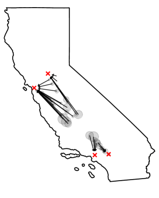
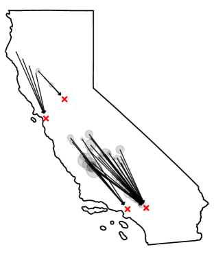
Figure 3: These two plots illustrate the special property of discrete Wasserstein barycenters proved in Theorem 2.1: there is no mass-splitting when optimally transporting the inventory at each barycenter support to the corresponding demand for each month. The image at left shows all the transported mass flowing from the optimal barycenter into San Francisco, Sacramento, Los Angeles and San Bernardino for month of March (the corresponding March demand is shown middle-left in Figure 1). The image at right shows the corresponding optimal transport for the month of July. Notice that these figures only show the barycenter support points which transport into the four cities shown here. The other barycenter supports transport goods to the other five cities not shown. We remark that Theorem 2.1 also establishes that transportation is balanced so that the transportation displacements sum to zero at each barycenter support point.

Proposition 1 guarantees that any barycenter P¯¯𝑃\bar{P} computed with discrete marginals has the form

P¯=𝐱Sz𝐱δ𝐱,z𝐱0.formulae-sequence¯𝑃subscript𝐱𝑆subscript𝑧𝐱subscript𝛿𝐱subscript𝑧𝐱subscriptabsent0\bar{P}=\sum_{{\bf x}\in S}z_{\bf x}\delta_{\bf x},\hskip 14.45377ptz_{\bf x}\in\mathbb{R}_{\geq 0}. (7)

Here δ𝐱subscript𝛿𝐱\delta_{\bf x} is the Dirac-δ𝛿\delta-function at 𝐱d𝐱superscript𝑑{\bf x}\in\mathbb{R}^{d} and z𝐱subscript𝑧𝐱z_{\bf x} corresponds to the mass (or probability) at 𝐱𝐱{\bf x}. This implies that any coupling of P¯¯𝑃\bar{P} with Pisubscript𝑃𝑖P_{i}, which realizes the Wasserstein distance, is in fact characterized by a finite matrix. Treating the coordinates of these matrices and the values z𝐱subscript𝑧𝐱z_{\bf x} as variables, the set of all solutions to (1) are obtained through a finite-dimensional linear program (see (23) below). In coo-14 a similar linear program was used to find approximate barycenters for sets of absolutely continuous measures by finitely approximating the support of P¯¯𝑃\bar{P} (which is sub-optimal for the continuous problem). Our use of the finite linear program characterization of P¯¯𝑃\bar{P} is different from continuous approximation. We use a version of the linear program to analyze properties of discrete barycenters themselves. Indeed, since the set of all discrete barycenters is on a face of the underlying polyhedron, one can study their properties by means of polyhedral theory.

Our first theorem illustrates a similarity between barycenters defined from absolutely continuous P1,,PNsubscript𝑃1subscript𝑃𝑁P_{1},\ldots,P_{N} and barycenters defined in the discrete setting. The results of ac-11 establish, in the absolutely continuous case, that there exist optimal transports from the barycenter to each Pisubscript𝑃𝑖P_{i} which are optimal in the sense of Wasserstein distance and are gradients of convex functions. Theorem 2.1 shows that such transports not only exist for discrete barycenters but also share similar properties.

Theorem 2.1

Suppose P1,,PNsubscript𝑃1subscript𝑃𝑁P_{1},\ldots,P_{N} are discrete probability measures. Let P¯¯𝑃\bar{P} denote a Wasserstein barycenter solution to (1) and let X𝑋X be a random variable with distribution P¯¯𝑃\bar{P}. Then there exist finite convex functions ψi:dd:subscript𝜓𝑖superscript𝑑superscript𝑑\psi_{i}:\mathbb{R}^{d}\rightarrow\mathbb{R}^{d}, for each i=1,,N𝑖1𝑁i=1,\ldots,N, such that

  1. i)

    ψi(P¯)=Pi, i.subscript𝜓𝑖¯𝑃subscript𝑃𝑖 for-all𝑖\displaystyle\nabla\psi_{i}(\bar{P})=P_{i},\text{ }\forall i.

  2. ii)

    E|Xψi(X)|2=W2(P¯,Pi)2, i.𝐸superscript𝑋subscript𝜓𝑖𝑋2subscript𝑊2superscript¯𝑃subscript𝑃𝑖2 for-all𝑖\displaystyle E|X-\nabla\psi_{i}(X)|^{2}=W_{2}(\bar{P},P_{i})^{2},\text{ }\forall i.

  3. iii)

    1Ni=1Nψi(xj)=xj, xjsupp(P¯).formulae-sequence1𝑁superscriptsubscript𝑖1𝑁subscript𝜓𝑖subscript𝑥𝑗subscript𝑥𝑗 for-allsubscript𝑥𝑗supp¯𝑃\displaystyle\frac{1}{N}\sum_{i=1}^{N}\nabla\psi_{i}(x_{j})=x_{j},\text{ }\forall x_{j}\in\text{supp}(\bar{P}).

  4. iv)

    1Ni=1Nψi(xj)=|xj|22, xjsupp(P¯).formulae-sequence1𝑁superscriptsubscript𝑖1𝑁subscript𝜓𝑖subscript𝑥𝑗superscriptsubscript𝑥𝑗22 for-allsubscript𝑥𝑗supp¯𝑃\displaystyle\frac{1}{N}\sum_{i=1}^{N}\psi_{i}(x_{j})=\frac{|x_{j}|^{2}}{2},\text{ }\forall x_{j}\in\text{supp}(\bar{P}).

Intuitively, one would expect the support of a barycenter to be large to accommodate such a condition. This is particularly plausible since such these transports must realize the Wasserstein distance between each measure and the barycenter. However, it has been noted that the barycenters of discrete measures are often sparse in practice; see for example cd-14 . Our second main result resolves this tension and establishes that there always is a Wasserstein barycenter whose solution is theoretically guaranteed to be sparse.

Theorem 2.2

Suppose P1,,PNsubscript𝑃1subscript𝑃𝑁P_{1},\ldots,P_{N} are discrete probability measures, and let Si=|supp(Pi)|subscript𝑆𝑖suppsubscript𝑃𝑖S_{i}=|\text{supp}(P_{i})|. Then there exists a barycenter P¯¯𝑃\bar{P} of these measures such that

|supp(P¯)|i=1NSiN+1.supp¯𝑃superscriptsubscript𝑖1𝑁subscript𝑆𝑖𝑁1|\text{supp}(\bar{P})|\leq\sum_{i=1}^{N}S_{i}-N+1. (8)

We would like to stress how low this guaranteed upper bound on the size of the support of the barycenter actually is. For example, let every Pisubscript𝑃𝑖P_{i} have a support of the same cardinality T𝑇T. Then |S|TN𝑆superscript𝑇𝑁|S|\leq T^{N} and if the support points are in general position one has |S|=TN𝑆superscript𝑇𝑁|S|=T^{N}. In contrast, the support of the barycenter has cardinality at most NT𝑁𝑇NT.

Additionally, the bound in Theorem 2.2 is the best possible in the sense that, for any natural numbers N𝑁N and W𝑊W, it is easy to come up with a set of N𝑁N measures for which |supp(P¯)|=i=1NSiN+1=Wsupp¯𝑃superscriptsubscript𝑖1𝑁subscript𝑆𝑖𝑁1𝑊|\text{supp}(\bar{P})|=\sum_{i=1}^{N}S_{i}-N+1=W: Choose P1subscript𝑃1P_{1} to have W𝑊W support points and uniformly distributed mass 1W1𝑊\frac{1}{W} on each of these points. Choose the other Pisubscript𝑃𝑖P_{i} to have a single support point of mass 111. Then |S|=W𝑆𝑊|S|=W and the barycenter uses all of these possible support points with mass 1W1𝑊\frac{1}{W}.

A particularly frequent setting in applications is that all the Pisubscript𝑃𝑖P_{i} are supported on the same discrete grid, uniform in all directions, in dsuperscript𝑑\mathbb{R}^{d}. See for example cd-14 ; rpdb-12 for applications in computer vision with d=2𝑑2d=2. In this situation, the set S𝑆S of possible centroids is a finer uniform grid in dsuperscript𝑑\mathbb{R}^{d}, which allows us to strengthen the results in Proposition 1 and Theorem 2.2.

Corollary 1

Let P1,,PNsubscript𝑃1subscript𝑃𝑁P_{1},\ldots,P_{N} be discrete probability measures supported on an L1××Ldsubscript𝐿1subscript𝐿𝑑L_{1}{\times}\ldots{\times}L_{d}-grid, uniform in all directions, in dsuperscript𝑑\mathbb{R}^{d}. Then there exists a barycenter P¯¯𝑃\bar{P} supported on a refined (N(L11)+1)××(N(Ld1)+1)𝑁subscript𝐿111𝑁subscript𝐿𝑑11(N(L_{1}-1)+1)\times\ldots\times(N(L_{d}-1)+1)-grid, uniform in all directions, with |supp(P¯)|N(i=1dLi1)+1supp¯𝑃𝑁superscriptsubscriptproduct𝑖1𝑑subscript𝐿𝑖11|\text{supp}(\bar{P})|\leq N(\prod\limits_{i=1}^{d}L_{i}-1)+1. In particular, the density of the support of the barycenter on this finer grid is less than

1Nd1i=1dLi(Li1).1superscript𝑁𝑑1superscriptsubscriptproduct𝑖1𝑑subscript𝐿𝑖subscript𝐿𝑖1\frac{1}{N^{d-1}}\prod\limits_{i=1}^{d}\frac{L_{i}}{(L_{i}-1)}.

3 Proofs

In this section we prove the results outlined in Section 2. We begin with a proof of Proposition 1.

3.1 Existence of Discrete Barycenters

Recall that a discrete barycenter P¯¯𝑃\bar{P} is an optimizer of (3)3(\ref{barycenter}) when P1,,PNsubscript𝑃1subscript𝑃𝑁P_{1},\ldots,P_{N} are discrete probability measures. We will show that P¯¯𝑃\bar{P} must have the form of a coordinatewise average of optimally coupled random vectors with marginals given by the Pisubscript𝑃𝑖P_{i}. In particular, we will establish the existence of N𝑁N random vectors X1o,,XNosuperscriptsubscript𝑋1𝑜superscriptsubscript𝑋𝑁𝑜X_{1}^{o},\ldots,X_{N}^{o} with marginal distributions XioPisimilar-tosuperscriptsubscript𝑋𝑖𝑜subscript𝑃𝑖X_{i}^{o}\sim P_{i} that are as highly correlated as possible so that the variability in the average Xo¯=X1o++XNoN¯superscript𝑋𝑜superscriptsubscript𝑋1𝑜superscriptsubscript𝑋𝑁𝑜𝑁\overline{X^{o}}=\frac{X_{1}^{o}+\cdots+X_{N}^{o}}{N} is maximized. Once these coupled random vectors X1o,,XNosuperscriptsubscript𝑋1𝑜superscriptsubscript𝑋𝑁𝑜X_{1}^{o},\ldots,X_{N}^{o} are obtained, the distribution of the average Xo¯¯superscript𝑋𝑜\overline{X^{o}} (denoted Xo¯¯superscript𝑋𝑜\mathcal{L}\overline{X^{o}}) will serve as P¯¯𝑃\bar{P}.

Proof (of Proposition 1)

As remarked earlier, part i) of Proposition 1 follows from the general results of Kellerer k-84 and Rachev r-84 . Therefore there exists an optimally coupled random vector (X1o,,XNo)Π(P1,,PN)superscriptsubscript𝑋1𝑜superscriptsubscript𝑋𝑁𝑜Πsubscript𝑃1subscript𝑃𝑁(X_{1}^{o},\ldots,X_{N}^{o})\in\Pi({P_{1},\ldots,P_{N}}) which satisfies (5). We will show that

i=1NW2(Xo¯,Pi)2=infP𝒫2(d)i=1NW2(P,Pi)2.superscriptsubscript𝑖1𝑁subscript𝑊2superscript¯superscript𝑋𝑜subscript𝑃𝑖2subscriptinfimum𝑃superscript𝒫2superscript𝑑superscriptsubscript𝑖1𝑁subscript𝑊2superscript𝑃subscript𝑃𝑖2\sum_{i=1}^{N}W_{2}\bigl{(}\mathcal{L}\overline{X^{o}},P_{i}\bigr{)}^{2}=\inf_{P\in\mathcal{P}^{2}(\mathbb{R}^{d})}\sum_{i=1}^{N}W_{2}(P,P_{i})^{2}. (9)

Notice the definition of S𝑆S automatically implies supp(Xo¯)Ssupp¯superscript𝑋𝑜𝑆\text{supp}(\mathcal{L}\overline{X^{o}})\subseteq S so that (9) will imply

i=1NW2(Xo¯,Pi)2=inf𝒫𝒮2(d)i=1NW2(P,Pi)2=infP𝒫2(d)i=1NW2(P,Pi)2superscriptsubscript𝑖1𝑁subscript𝑊2superscript¯superscript𝑋𝑜subscript𝑃𝑖2subscriptinfimumsuperscriptsubscript𝒫𝒮2superscript𝑑superscriptsubscript𝑖1𝑁subscript𝑊2superscript𝑃subscript𝑃𝑖2subscriptinfimum𝑃superscript𝒫2superscript𝑑superscriptsubscript𝑖1𝑁subscript𝑊2superscript𝑃subscript𝑃𝑖2\sum_{i=1}^{N}W_{2}\bigl{(}\mathcal{L}\overline{X^{o}},P_{i}\bigr{)}^{2}=\inf_{\mathcal{P}_{\mathcal{S}}^{2}(\mathbb{R}^{d})}\sum_{i=1}^{N}W_{2}(P,P_{i})^{2}=\inf_{P\in\mathcal{P}^{2}(\mathbb{R}^{d})}\sum_{i=1}^{N}W_{2}(P,P_{i})^{2} (10)

and complete the proof of part ii).

So suppose P𝒫2(d)𝑃superscript𝒫2superscript𝑑P\in\mathcal{P}^{2}(\mathbb{R}^{d}). Then for all i=1,,N𝑖1𝑁i=1,\ldots,N there exists an optimally coupled random vector (Yi,Xi)Π(P,Pi)subscriptsuperscript𝑌𝑖superscriptsubscript𝑋𝑖Π𝑃subscript𝑃𝑖(Y^{*}_{i},X_{i}^{*})\in\Pi(P,P_{i}) such that W2(P,Pi)2=E|YiXi|2subscript𝑊2superscript𝑃subscript𝑃𝑖2𝐸superscriptsubscriptsuperscript𝑌𝑖superscriptsubscript𝑋𝑖2W_{2}(P,P_{i})^{2}=E|Y^{*}_{i}-X_{i}^{*}|^{2}. (This is a well known property of the Wasserstein distance W2subscript𝑊2W_{2}, see for example Proposition 2.1 in v-03 .) Since the random variables Y1,,YNsubscriptsuperscript𝑌1subscriptsuperscript𝑌𝑁Y^{*}_{1},\ldots,Y^{*}_{N} all have distribution P𝑃P it is easy to see that there exists a generalized Gluing lemma for the existence of a random vector (Y,X1,,XN)Π(P,P1,,PN)𝑌subscript𝑋1subscript𝑋𝑁Π𝑃subscript𝑃1subscript𝑃𝑁(Y,X_{1},\ldots,X_{N})\in\Pi(P,P_{1},\ldots,P_{N}) such that (Y,Xi)𝑌subscript𝑋𝑖(Y,X_{i}) has the same distribution as (Y,Xi)superscript𝑌superscriptsubscript𝑋𝑖(Y^{*},X_{i}^{*}) for each i𝑖i. This can be seeing by first sampling a single YPsimilar-to𝑌𝑃Y\sim P then sample X1,,XNsubscript𝑋1subscript𝑋𝑁X_{1},\ldots,X_{N} independently conditional on Y𝑌Y where the conditional distribution Pr(Xi=x|Y=y)𝑃𝑟subscript𝑋𝑖conditional𝑥𝑌𝑦Pr(X_{i}=x|Y=y) is set to Pr(Xi=x|Y=y)𝑃𝑟superscriptsubscript𝑋𝑖conditional𝑥superscript𝑌𝑦Pr(X_{i}^{*}=x|Y^{*}=y) (the finite support of P1,,PNsubscript𝑃1subscript𝑃𝑁P_{1},\ldots,P_{N} is sufficient to guarantee existence of these conditional distributions). This yields

1Ni=1NW2(P,Pi)2=1Ni=1NE|YiXi|2=1Ni=1NE|YXi|2.1𝑁superscriptsubscript𝑖1𝑁subscript𝑊2superscript𝑃subscript𝑃𝑖21𝑁superscriptsubscript𝑖1𝑁𝐸superscriptsuperscriptsubscript𝑌𝑖subscriptsuperscript𝑋𝑖21𝑁superscriptsubscript𝑖1𝑁𝐸superscript𝑌subscript𝑋𝑖2\frac{1}{N}\sum_{i=1}^{N}W_{2}(P,P_{i})^{2}=\frac{1}{N}\sum_{i=1}^{N}E|Y_{i}^{*}-X^{*}_{i}|^{2}=\frac{1}{N}\sum_{i=1}^{N}E|Y-X_{i}|^{2}. (11)

Now note that XiPisimilar-tosubscript𝑋𝑖subscript𝑃𝑖X_{i}\sim P_{i} and XioPisimilar-tosuperscriptsubscript𝑋𝑖𝑜subscript𝑃𝑖X_{i}^{o}\sim P_{i}. Thus

i=1NE|Xo¯Xio|2superscriptsubscript𝑖1𝑁𝐸superscript¯superscript𝑋𝑜subscriptsuperscript𝑋𝑜𝑖2\displaystyle\sum_{i=1}^{N}E\bigl{|}\overline{X^{o}}-X^{o}_{i}\bigr{|}^{2} =i=1NE|Xo¯|22Ei=1NXo¯,Xio+i=1NE|Xio|2=NE|Xo¯|2+i=1NE|Xio|2\displaystyle=\sum_{i=1}^{N}E\bigl{|}\overline{X^{o}}\bigr{|}^{2}-2E\sum_{i=1}^{N}\langle\overline{X^{o}},X^{o}_{i}\rangle+\sum_{i=1}^{N}E\bigl{|}X^{o}_{i}\bigl{|}^{2}=-NE\bigl{|}\overline{X^{o}}\bigr{|}^{2}+\sum_{i=1}^{N}E\bigl{|}X^{o}_{i}\bigl{|}^{2}
=NE|Xo¯|2+i=1NE|Xi|2=inf (X1,,XN) Π(P1,,PN) NE|X¯|2+i=1NE|Xi|2\displaystyle=-NE\bigl{|}\overline{X^{o}}\bigr{|}^{2}+\sum_{i=1}^{N}E\bigl{|}X_{i}\bigl{|}^{2}=\inf_{\shortstack{\scriptsize$(X_{1},\ldots,X_{N})$\\ \scriptsize$\quad\quad\in\Pi({P}_{1},\ldots,{P}_{N})$ }}-NE\bigl{|}\overline{X}\bigr{|}^{2}+\sum_{i=1}^{N}E\bigl{|}X_{i}\bigl{|}^{2}
=inf (X1,,XN) Π(P1,,PN) i=1NE|X¯|22Ei=1NX¯,Xi+i=1NE|Xi|2\displaystyle=\inf_{\shortstack{\scriptsize$(X_{1},\ldots,X_{N})$\\ \scriptsize$\quad\quad\in\Pi({P}_{1},\ldots,{P}_{N})$ }}\sum_{i=1}^{N}E\bigl{|}\overline{X}\bigr{|}^{2}-2E\sum_{i=1}^{N}\langle\overline{X},X_{i}\rangle+\sum_{i=1}^{N}E\bigl{|}X_{i}\bigl{|}^{2}
=inf (X1,,XN) Π(P1,,PN) i=1NE|X¯Xi|2.absentsubscriptinfimum (X1,,XN) Π(P1,,PN) superscriptsubscript𝑖1𝑁𝐸superscript¯𝑋subscript𝑋𝑖2\displaystyle=\inf_{\shortstack{\scriptsize$(X_{1},\ldots,X_{N})$\\ \scriptsize$\quad\quad\in\Pi(P_{1},\ldots,P_{N})$ }}\sum_{i=1}^{N}E\bigl{|}\overline{X}-X_{i}\bigr{|}^{2}. (12)

Also, note that

E|Xo¯Xio|2inf(Y,X)Π(Xo¯,Pi)E|YX|2=W2(Xo¯,Pi)2.𝐸superscript¯superscript𝑋𝑜subscriptsuperscript𝑋𝑜𝑖2subscriptinfimum𝑌𝑋Π¯superscript𝑋𝑜subscript𝑃𝑖𝐸superscript𝑌𝑋2subscript𝑊2superscript¯superscript𝑋𝑜subscript𝑃𝑖2E|\overline{X^{o}}-X^{o}_{i}|^{2}\geq\inf_{(Y,X)\in\Pi(\mathcal{L}\overline{X^{o}},P_{i})}E|Y-X|^{2}=W_{2}(\mathcal{L}\overline{X^{o}},P_{i})^{2}. (13)

Combining (3.1)3.1(\ref{hugeThing}) and (13)13(\ref{smallThing}), we get

1Ni=1NE|X¯Xi|21Ni=1NE|Xo¯Xio|21Ni=1NW2(Xo¯,Pi)2.1𝑁superscriptsubscript𝑖1𝑁𝐸superscript¯𝑋subscript𝑋𝑖21𝑁superscriptsubscript𝑖1𝑁𝐸superscript¯superscript𝑋𝑜subscriptsuperscript𝑋𝑜𝑖21𝑁superscriptsubscript𝑖1𝑁subscript𝑊2superscript¯superscript𝑋𝑜subscript𝑃𝑖2\frac{1}{N}\sum_{i=1}^{N}E|\overline{X}-X_{i}|^{2}\geq\frac{1}{N}\sum_{i=1}^{N}E|\overline{X^{o}}-X^{o}_{i}|^{2}\geq\frac{1}{N}\sum_{i=1}^{N}W_{2}(\mathcal{L}\overline{X^{o}},P_{i})^{2}. (14)

Further we have a minorant for the right hand side of (11) as follows

1Ni=1NE|YXi|21𝑁superscriptsubscript𝑖1𝑁𝐸superscript𝑌subscript𝑋𝑖2\displaystyle\frac{1}{N}\sum_{i=1}^{N}E|Y-X_{i}|^{2} =1Ni=1NE|YX¯+X¯Xi|2absent1𝑁superscriptsubscript𝑖1𝑁𝐸superscript𝑌¯𝑋¯𝑋subscript𝑋𝑖2\displaystyle=\frac{1}{N}\sum_{i=1}^{N}E|Y-\overline{X}+\overline{X}-X_{i}|^{2}
=1Ni=1NE|YX¯|2+2NEi=1NYX¯,X¯Xi+1Ni=1NE|X¯Xi|2absent1𝑁superscriptsubscript𝑖1𝑁𝐸superscript𝑌¯𝑋22𝑁𝐸superscriptsubscript𝑖1𝑁𝑌¯𝑋¯𝑋subscript𝑋𝑖1𝑁superscriptsubscript𝑖1𝑁𝐸superscript¯𝑋subscript𝑋𝑖2\displaystyle=\frac{1}{N}\sum_{i=1}^{N}E|Y-\overline{X}|^{2}+\frac{2}{N}E\sum_{i=1}^{N}\langle Y-\overline{X},\overline{X}-X_{i}\rangle+\frac{1}{N}\sum_{i=1}^{N}E|\overline{X}-X_{i}|^{2}
=E|YX¯|2+2NEYX¯,i=1N(X¯Xi)+1Ni=1NE|X¯Xi|2absent𝐸superscript𝑌¯𝑋22𝑁𝐸𝑌¯𝑋superscriptsubscript𝑖1𝑁¯𝑋subscript𝑋𝑖1𝑁superscriptsubscript𝑖1𝑁𝐸superscript¯𝑋subscript𝑋𝑖2\displaystyle=E|Y-\overline{X}|^{2}+\frac{2}{N}E\langle Y-\overline{X},\sum_{i=1}^{N}(\overline{X}-X_{i})\rangle+\frac{1}{N}\sum_{i=1}^{N}E|\overline{X}-X_{i}|^{2}
=E|YX¯|2+1Ni=1NE|X¯Xi|21Ni=1NE|X¯Xi|2.absent𝐸superscript𝑌¯𝑋21𝑁superscriptsubscript𝑖1𝑁𝐸superscript¯𝑋subscript𝑋𝑖21𝑁superscriptsubscript𝑖1𝑁𝐸superscript¯𝑋subscript𝑋𝑖2\displaystyle=E|Y-\overline{X}|^{2}+\frac{1}{N}\sum_{i=1}^{N}E|\overline{X}-X_{i}|^{2}\geq\frac{1}{N}\sum_{i=1}^{N}E|\overline{X}-X_{i}|^{2}. (15)

Putting (11), (14), and (15) together we obtain

1Ni=1NW2(P,Pi)2=1Ni=1NE|YXi|21Ni=1NE|X¯Xi|21Ni=1NW2(Xo¯,Pi)2.1𝑁superscriptsubscript𝑖1𝑁subscript𝑊2superscript𝑃subscript𝑃𝑖21𝑁superscriptsubscript𝑖1𝑁𝐸superscript𝑌subscript𝑋𝑖21𝑁superscriptsubscript𝑖1𝑁𝐸superscript¯𝑋subscript𝑋𝑖21𝑁superscriptsubscript𝑖1𝑁subscript𝑊2superscript¯superscript𝑋𝑜subscript𝑃𝑖2\frac{1}{N}\sum_{i=1}^{N}W_{2}(P,P_{i})^{2}=\frac{1}{N}\sum_{i=1}^{N}E|Y-X_{i}|^{2}\geq\frac{1}{N}\sum_{i=1}^{N}E|\overline{X}-X_{i}|^{2}\geq\frac{1}{N}\sum_{i=1}^{N}W_{2}(\mathcal{L}\overline{X^{o}},P_{i})^{2}. (16)

This shows that Xo¯¯superscript𝑋𝑜\mathcal{L}\overline{X^{o}} is a minimizer of our problem and hence a barycenter, proving part i).

Finally, to prove part iii), note that if P𝒫2(d)𝑃superscript𝒫2superscript𝑑P\in\mathcal{P}^{2}(\mathbb{R}^{d}) and supp(P)Snot-subset-of-nor-equalssupp𝑃𝑆\text{supp}(P)\nsubseteq S, then any coupling (Y,X1,,XN)Π(P,P1,,PN)𝑌subscript𝑋1subscript𝑋𝑁Π𝑃subscript𝑃1subscript𝑃𝑁(Y,X_{1},\ldots,X_{N})\in\Pi(P,P_{1},\ldots,P_{N}) must satisfy E|YX¯|2>0𝐸superscript𝑌¯𝑋20E|Y-\overline{X}|^{2}>0 (since supp(X¯)Ssupp¯𝑋𝑆\text{supp}(\overline{X})\subseteq S and supp(P)Snot-subset-of-nor-equalssupp𝑃𝑆\text{supp}(P)\nsubseteq S). This implies, by the last line of (15), that

1Ni=1NE|YXi|2>1Ni=1NE|X¯Xi|2,1𝑁superscriptsubscript𝑖1𝑁𝐸superscript𝑌subscript𝑋𝑖21𝑁superscriptsubscript𝑖1𝑁𝐸superscript¯𝑋subscript𝑋𝑖2\frac{1}{N}\sum_{i=1}^{N}E|Y-X_{i}|^{2}>\frac{1}{N}\sum_{i=1}^{N}E|\overline{X}-X_{i}|^{2}, (17)

and hence that

1Ni=1NW2(P,Pi)2=1Ni=1NE|YXi|2>1Ni=1NE|X¯Xi|21Ni=1NW2(Xo¯,Pi)2,1𝑁superscriptsubscript𝑖1𝑁subscript𝑊2superscript𝑃subscript𝑃𝑖21𝑁superscriptsubscript𝑖1𝑁𝐸superscript𝑌subscript𝑋𝑖21𝑁superscriptsubscript𝑖1𝑁𝐸superscript¯𝑋subscript𝑋𝑖21𝑁superscriptsubscript𝑖1𝑁subscript𝑊2superscript¯superscript𝑋𝑜subscript𝑃𝑖2\frac{1}{N}\sum_{i=1}^{N}W_{2}(P,P_{i})^{2}=\frac{1}{N}\sum_{i=1}^{N}E|Y-X_{i}|^{2}>\frac{1}{N}\sum_{i=1}^{N}E|\overline{X}-X_{i}|^{2}\geq\frac{1}{N}\sum_{i=1}^{N}W_{2}(\mathcal{L}\overline{X^{o}},P_{i})^{2}, (18)

so that P𝑃P is not a barycenter. Therefore for any barycenter P¯¯𝑃\bar{P}, we must have supp(P¯)Ssupp¯𝑃𝑆\text{supp}(\bar{P})\subseteq S, which proves part iii). ∎

3.2 Linear Programming and Optimal Transport

Let us now develop a linear programming model (LP) for the exact computation of a discrete barycenter. Suppose we have a set of discrete measures Pisubscript𝑃𝑖P_{i}, i=1,,N𝑖1𝑁i=1,\ldots,N, and additionally another discrete measure P𝑃P. Let S0=|supp(P)|subscript𝑆0supp𝑃S_{0}=|\text{supp}(P)| and Si=|supp(Pi)|subscript𝑆𝑖suppsubscript𝑃𝑖S_{i}=|\text{supp}(P_{i})| for each i𝑖i as before. Let xjsubscript𝑥𝑗x_{j}, j=1,,S0𝑗1subscript𝑆0j=1,\ldots,S_{0} be the points in the support of P𝑃P, each with mass djsubscript𝑑𝑗d_{j}, and let xiksubscript𝑥𝑖𝑘x_{ik}, k=1,,Si𝑘1subscript𝑆𝑖k=1,\ldots,S_{i} be the points in the support of Pisubscript𝑃𝑖P_{i}, each with mass diksubscript𝑑𝑖𝑘d_{ik}. For the sake of a simple notation in the following, when summing over these values, the indices take the full range unless stated otherwise.

If (X,Yi)Π(P,Pi)𝑋subscript𝑌𝑖Π𝑃subscript𝑃𝑖(X,Y_{i})\in\Pi(P,P_{i}), then this coupling can be viewed as a finite matrix, since both probability measures are discrete. We define yijk0subscript𝑦𝑖𝑗𝑘0y_{ijk}\geq 0 to be the value of the entry corresponding to the margins xjsubscript𝑥𝑗x_{j} and xiksubscript𝑥𝑖𝑘x_{ik} in this finite matrix.

Note in this coupling that kyijk=djsubscript𝑘subscript𝑦𝑖𝑗𝑘subscript𝑑𝑗\sum_{k}y_{ijk}=d_{j} for all j𝑗j and that jyijk=diksubscript𝑗subscript𝑦𝑖𝑗𝑘subscript𝑑𝑖𝑘\sum_{j}y_{ijk}=d_{ik} for all k𝑘k and further that

E|XY|2=j,k|xjxik|2yijk=j,kcijkyijk,𝐸superscript𝑋𝑌2subscript𝑗𝑘superscriptsubscript𝑥𝑗subscript𝑥𝑖𝑘2subscript𝑦𝑖𝑗𝑘subscript𝑗𝑘subscript𝑐𝑖𝑗𝑘subscript𝑦𝑖𝑗𝑘E|X-Y|^{2}=\sum_{j,k}|x_{j}-x_{ik}|^{2}\cdot y_{ijk}=\sum_{j,k}c_{ijk}\cdot y_{ijk}, (19)

where cijk:=|xjxik|2assignsubscript𝑐𝑖𝑗𝑘superscriptsubscript𝑥𝑗subscript𝑥𝑖𝑘2c_{ijk}:=|x_{j}-x_{ik}|^{2} just by definition.

Given a non-negative vector 𝐲=(yijk)0𝐲subscript𝑦𝑖𝑗𝑘0{\bf y}=(y_{ijk})\geq 0 that satisfies kyijk=djsubscript𝑘subscript𝑦𝑖𝑗𝑘subscript𝑑𝑗\sum_{k}y_{ijk}=d_{j} for all i𝑖i and j𝑗j and jyijk=diksubscript𝑗subscript𝑦𝑖𝑗𝑘subscript𝑑𝑖𝑘\sum_{j}y_{ijk}=d_{ik} for all i𝑖i and k𝑘k, we call 𝐲𝐲{\bf y} an N-star transport between P𝑃P and the Pisubscript𝑃𝑖P_{i}. We define the cost of this transport to be c(𝐲):=i,j,kcijkyijkassign𝑐𝐲subscript𝑖𝑗𝑘subscript𝑐𝑖𝑗𝑘subscript𝑦𝑖𝑗𝑘c({\bf y}):=\sum_{i,j,k}c_{ijk}\cdot y_{ijk}.

Further there exist vectors (X,Yi)Π(P,Pi)superscript𝑋superscriptsubscript𝑌𝑖Π𝑃subscript𝑃𝑖(X^{*},Y_{i}^{*})\in\Pi(P,P_{i}) for all i𝑖i, and a corresponding N𝑁N-star transport 𝐲superscript𝐲{\bf y^{*}}, such that

iW2(P,Pi)2=iE|XY|2=c(𝐲).subscript𝑖subscript𝑊2superscript𝑃subscript𝑃𝑖2subscript𝑖𝐸superscriptsuperscript𝑋superscript𝑌2𝑐superscript𝐲\sum_{i}W_{2}(P,P_{i})^{2}=\sum_{i}E|X^{*}-Y^{*}|^{2}=c({\bf y^{*}}). (20)

For any (X,Yi)Π(P,Pi)𝑋subscript𝑌𝑖Π𝑃subscript𝑃𝑖(X,Y_{i})\in\Pi(P,P_{i}) we also have E|XYi|2E|XYi|2𝐸superscriptsuperscript𝑋superscriptsubscript𝑌𝑖2𝐸superscript𝑋subscript𝑌𝑖2E|X^{*}-Y_{i}^{*}|^{2}\leq E|X-Y_{i}|^{2}, and hence it is easily seen that 𝐲superscript𝐲{\bf y^{*}} is an optimizer to the following linear program

min𝐲subscript𝐲\displaystyle\min_{\bf y}  c(𝐲) 𝑐𝐲\displaystyle\text{ }\text{ }c({\bf y})
kyijk=subscript𝑘subscript𝑦𝑖𝑗𝑘absent\displaystyle\sum_{k}y_{ijk}=  dj,  i=1,,N, j=1,,S0,formulae-sequence subscript𝑑𝑗  for-all𝑖1𝑁 for-all𝑗1subscript𝑆0\displaystyle\text{ }\text{ }d_{j},\text{ }\text{ }\forall i=1,\ldots,N,\text{ }\forall j=1,\ldots,S_{0},
jyijk=subscript𝑗subscript𝑦𝑖𝑗𝑘absent\displaystyle\sum_{j}y_{ijk}=  dik,  i=1,,N, k=1,,Si,formulae-sequence subscript𝑑𝑖𝑘  for-all𝑖1𝑁 for-all𝑘1subscript𝑆𝑖\displaystyle\text{ }\text{ }d_{ik},\text{ }\text{ }\forall i=1,\ldots,N,\text{ }\forall k=1,\ldots,S_{i}, (21)
yijksubscript𝑦𝑖𝑗𝑘absent\displaystyle y_{ijk}\geq  0,     i=1,,N, j=1,,S0, k=1,,Si.formulae-sequence 0     for-all𝑖1𝑁 for-all𝑗1subscript𝑆0 for-all𝑘1subscript𝑆𝑖\displaystyle\text{ }\text{ }0,\text{ }\text{ }\text{ }\text{ }\text{ }\forall i=1,\ldots,N,\text{ }\forall j=1,\ldots,S_{0},\text{ }\forall k=1,\ldots,S_{i}.

Now suppose we wish to find a barycenter using a linear program. Then using Proposition 1 we know that this amounts to finding a solution to

minP𝒫𝒮2(d)i=1NW2(P,Pi)2,P=𝐱Sz𝐱δ𝐱,z𝐱0.formulae-sequencesubscript𝑃superscriptsubscript𝒫𝒮2superscript𝑑superscriptsubscript𝑖1𝑁subscript𝑊2superscript𝑃subscript𝑃𝑖2𝑃subscript𝐱𝑆subscript𝑧𝐱subscript𝛿𝐱subscript𝑧𝐱subscriptabsent0\min_{P\in\mathcal{P}_{\mathcal{S}}^{2}(\mathbb{R}^{d})}\sum_{i=1}^{N}W_{2}(P,P_{i})^{2},\hskip 36.135ptP=\sum_{{\bf x}\in S}z_{\bf x}\delta_{\bf x},\hskip 14.45377ptz_{\bf x}\in\mathbb{R}_{\geq 0}. (22)

Using this we can expand the possible support of P𝑃P in the previous LP to S𝑆S, and let the mass at each xjSsubscript𝑥𝑗𝑆x_{j}\in S be represented by a variable zj0subscript𝑧𝑗0z_{j}\geq 0. This is a probability distribution if and only if the constraint jzj=1subscript𝑗subscript𝑧𝑗1\sum_{j}z_{j}=1 is satisfied. Then every exact barycenter, up to measure-zero sets, must be represented by some assignment of these variables and hence is an optimizer of the LP

min𝐲,𝐳subscript𝐲𝐳\displaystyle\min_{\bf y,z}  c(𝐲) 𝑐𝐲\displaystyle\text{ }\text{ }c({\bf y})
kyijk=subscript𝑘subscript𝑦𝑖𝑗𝑘absent\displaystyle\sum_{k}y_{ijk}=  zj,  i=1,,N, j=1,,S0,formulae-sequence subscript𝑧𝑗  for-all𝑖1𝑁 for-all𝑗1subscript𝑆0\displaystyle\text{ }\text{ }z_{j},\text{ }\text{ }\forall i=1,\ldots,N,\text{ }\forall j=1,\ldots,S_{0},
jyijk=subscript𝑗subscript𝑦𝑖𝑗𝑘absent\displaystyle\sum_{j}y_{ijk}=  dik,  i=1,,N, k=1,,Si,formulae-sequence subscript𝑑𝑖𝑘  for-all𝑖1𝑁 for-all𝑘1subscript𝑆𝑖\displaystyle\text{ }\text{ }d_{ik},\text{ }\text{ }\forall i=1,\ldots,N,\text{ }\forall k=1,\ldots,S_{i},
yijksubscript𝑦𝑖𝑗𝑘absent\displaystyle y_{ijk}\geq  0,     i=1,,N, j=1,,S0, k=1,,Si,formulae-sequence 0     for-all𝑖1𝑁 for-all𝑗1subscript𝑆0 for-all𝑘1subscript𝑆𝑖\displaystyle\text{ }\text{ }0,\text{ }\text{ }\text{ }\text{ }\text{ }\forall i=1,\ldots,N,\text{ }\forall j=1,\ldots,S_{0},\text{ }\forall k=1,\ldots,S_{i},
zjsubscript𝑧𝑗absent\displaystyle z_{j}\geq  0,     j=1,,S0.formulae-sequence 0     for-all𝑗1subscript𝑆0\displaystyle\text{ }\text{ }0,\text{ }\text{ }\text{ }\text{ }\text{ }\forall j=1,\ldots,S_{0}. (23)

Since each Pisubscript𝑃𝑖P_{i} is a probability distribution it is easy to see that jzj=1subscript𝑗subscript𝑧𝑗1\sum_{j}z_{j}=1 is just a consequence of satisfaction of the other constraints. Any optimizer (𝐲,𝐳)superscript𝐲superscript𝐳({\bf y^{*}},{\bf z^{*}}) to this LP is a barycenter P¯¯𝑃\bar{P} in that

minP𝒫𝒮2(d)i=1NW2(P,Pi)2=i=1NW2(P¯,Pi)2=c(𝐲) and P¯=jzjδxj.formulae-sequencesubscript𝑃superscriptsubscript𝒫𝒮2superscript𝑑superscriptsubscript𝑖1𝑁subscript𝑊2superscript𝑃subscript𝑃𝑖2superscriptsubscript𝑖1𝑁subscript𝑊2superscript¯𝑃subscript𝑃𝑖2𝑐superscript𝐲 and ¯𝑃subscript𝑗subscriptsuperscript𝑧𝑗subscript𝛿subscript𝑥𝑗\min_{P\in\mathcal{P}_{\mathcal{S}}^{2}(\mathbb{R}^{d})}\sum_{i=1}^{N}W_{2}(P,P_{i})^{2}=\sum_{i=1}^{N}W_{2}(\bar{P},P_{i})^{2}=c({\bf y^{*}})\hskip 21.68121pt\text{ and }\hskip 21.68121pt\bar{P}=\sum_{j}z^{*}_{j}\delta_{x_{j}}. (24)

It is notable that the LP in (23)23(\ref{LPequ}) corresponds to N𝑁N transportation problems, linked together with variables zjsubscript𝑧𝑗z_{j}, representing a common marginal for each transportation problem. In fact it is not hard to show that in the case N=2𝑁2N=2 this LP can be replaced with a network flow LP on a directed graph. It is easily seen that this LP is both bounded (it is a minimization of a positive linear sum of non-negative variables) and feasible (assign an arbitary zj=1subscript𝑧𝑗1z_{j}=1 and the remainder of them 00 and this reduces to solving N𝑁N transportation LPs). Thus it becomes useful to write down the dual LP, which also bares similarity to a dual transportation problem

maxτ,θsubscript𝜏𝜃\displaystyle\max_{\bf\tau,\theta}  i,kdikτik subscript𝑖𝑘subscript𝑑𝑖𝑘subscript𝜏𝑖𝑘\displaystyle\text{ }\text{ }\sum_{i,k}d_{ik}\cdot\tau_{ik}
θij+τiksubscript𝜃𝑖𝑗subscript𝜏𝑖𝑘absent\displaystyle\theta_{ij}+\tau_{ik}\leq  cijk,  i=1,,N, j=1,,S0, k=1,,Si,formulae-sequence subscript𝑐𝑖𝑗𝑘  for-all𝑖1𝑁 for-all𝑗1subscript𝑆0 for-all𝑘1subscript𝑆𝑖\displaystyle\text{ }\text{ }c_{ijk},\text{ }\text{ }\forall i=1,\ldots,N,\text{ }\forall j=1,\ldots,S_{0},\text{ }\forall k=1,\ldots,S_{i},
jθijsubscript𝑗subscript𝜃𝑖𝑗absent\displaystyle\sum_{j}\theta_{ij}\geq  0,     i=1,,N, j=1,,S0,formulae-sequence 0     for-all𝑖1𝑁 for-all𝑗1subscript𝑆0\displaystyle\text{ }\text{ }0,\text{ }\text{ }\text{ }\text{ }\text{ }\forall i=1,\ldots,N,\text{ }\forall j=1,\ldots,S_{0}, (25)

where there is a variable τiksubscript𝜏𝑖𝑘\tau_{ik} for each defining measure i𝑖i and each xiksupp(Pi)subscript𝑥𝑖𝑘suppsubscript𝑃𝑖x_{ik}\in\text{supp}(P_{i}) and a variable θijsubscript𝜃𝑖𝑗\theta_{ij} for each defining measure i𝑖i and each xjSsubscript𝑥𝑗𝑆x_{j}\in S.

These LPs not only will be used for computations in Section 4, but also can be used to develop the necessary theory for Theorem 2.1.

Lemma 1

Let P1,,PNsubscript𝑃1subscript𝑃𝑁P_{1},\ldots,P_{N} be discrete probability measures with a barycenter P¯¯𝑃\bar{P} given by a solution (𝐲,𝐳)superscript𝐲superscript𝐳({\bf y^{*}},{\bf z^{*}}) to (23). Then

  1. i)

    For any xjsupp(P¯)subscript𝑥𝑗supp¯𝑃x_{j}\in\text{supp}(\bar{P}) (i.e. zj>0superscriptsubscript𝑧𝑗0z_{j}^{*}>0) combined with any choice of xikisupp(Pi)subscript𝑥𝑖subscript𝑘𝑖suppsubscript𝑃𝑖x_{ik_{i}}\in\text{supp}(P_{i}) for i=1,,N𝑖1𝑁i=1,\ldots,N such that yijki>0subscriptsuperscript𝑦𝑖𝑗subscript𝑘𝑖0y^{*}_{ijk_{i}}>0 for each i𝑖i, one then has xj=1Nixikisubscript𝑥𝑗1𝑁subscript𝑖subscript𝑥𝑖subscript𝑘𝑖x_{j}=\frac{1}{N}\sum_{i}x_{ik_{i}}.

  2. ii)

    For any xjsupp(P¯)subscript𝑥𝑗supp¯𝑃x_{j}\in\text{supp}(\bar{P}) and i=1,,N𝑖1𝑁i=1,\ldots,N, one has |{yijk>0| xiksupp(Pi)}|=1conditional-setsubscriptsuperscript𝑦𝑖𝑗𝑘0 subscript𝑥𝑖𝑘suppsubscript𝑃𝑖1\big{|}\;\{y^{*}_{ijk}>0|\text{ }x_{ik}\in\text{supp}(P_{i})\}\;\big{|}=1.

Proof

i) Suppose the statement in i) is false. Then there exists an xj0supp(P¯)subscript𝑥subscript𝑗0supp¯𝑃x_{j_{0}}\in\text{supp}(\bar{P}) and there are points xikisupp(Pi)subscript𝑥𝑖subscript𝑘𝑖suppsubscript𝑃𝑖x_{ik_{i}}\in\text{supp}(P_{i}) for i=1,,N𝑖1𝑁i=1,\ldots,N such that yij0ki>0subscriptsuperscript𝑦𝑖subscript𝑗0subscript𝑘𝑖0y^{*}_{ij_{0}k_{i}}>0 for each i𝑖i and xj01Nixikisubscript𝑥subscript𝑗01𝑁subscript𝑖subscript𝑥𝑖subscript𝑘𝑖x_{j_{0}}\neq\frac{1}{N}\sum_{i}x_{ik_{i}}.

Let α=miniyij0ki>0𝛼subscript𝑖subscriptsuperscript𝑦𝑖subscript𝑗0subscript𝑘𝑖0\alpha=\min_{i}y^{*}_{ij_{0}k_{i}}>0 and let xj=1Nixikisubscript𝑥superscript𝑗1𝑁subscript𝑖subscript𝑥𝑖subscript𝑘𝑖x_{j^{*}}=\frac{1}{N}\sum_{i}x_{ik_{i}}. Then define (𝐲^,𝐳^)^𝐲^𝐳({\bf\hat{y}},{\bf\hat{z}}) such that y^ij0ki=yij0kiαsubscript^𝑦𝑖subscript𝑗0subscript𝑘𝑖subscriptsuperscript𝑦𝑖subscript𝑗0subscript𝑘𝑖𝛼\hat{y}_{ij_{0}k_{i}}=y^{*}_{ij_{0}k_{i}}-\alpha for each i𝑖i, y^ijki=yijki+αsubscript^𝑦𝑖superscript𝑗subscript𝑘𝑖subscriptsuperscript𝑦𝑖superscript𝑗subscript𝑘𝑖𝛼\hat{y}_{ij^{*}k_{i}}=y^{*}_{ij^{*}k_{i}}+\alpha for each i𝑖i, z^j0=zj0αsubscript^𝑧subscript𝑗0subscriptsuperscript𝑧subscript𝑗0𝛼\hat{z}_{j_{0}}=z^{*}_{j_{0}}-\alpha, z^j=zj+αsubscript^𝑧superscript𝑗subscriptsuperscript𝑧superscript𝑗𝛼\hat{z}_{j^{*}}=z^{*}_{j^{*}}+\alpha, and z^j=zjsubscript^𝑧𝑗subscriptsuperscript𝑧𝑗\hat{z}_{j}=z^{*}_{j} and y^ijk=yijksubscript^𝑦𝑖𝑗𝑘subscriptsuperscript𝑦𝑖𝑗𝑘\hat{y}_{ijk}=y^{*}_{ijk} for all other variables.

It is easily checked that (𝐲^,𝐳^)^𝐲^𝐳({\bf\hat{y}},{\bf\hat{z}}) is also a feasible solution to (23). Further

c(𝐲^)=c(𝐲)+α(icijkiicij0ki)<c(𝐲),𝑐^𝐲𝑐superscript𝐲𝛼subscript𝑖subscript𝑐𝑖superscript𝑗subscript𝑘𝑖subscript𝑖subscript𝑐𝑖subscript𝑗0subscript𝑘𝑖𝑐superscript𝐲c({\bf\hat{y}})=c({\bf y^{*}})+\alpha\left(\sum_{i}c_{ij^{*}k_{i}}-\sum_{i}c_{ij_{0}k_{i}}\right)<c({\bf y^{*}}), (26)

where the strict inequality follows since xj01Nixiki=xjsubscript𝑥subscript𝑗01𝑁subscript𝑖subscript𝑥𝑖subscript𝑘𝑖subscript𝑥superscript𝑗x_{j_{0}}\neq\frac{1}{N}\sum_{i}x_{ik_{i}}=x_{j^{*}} and therefore

icij0ki=i|xj0xiki|2>i|xjxiki|2=icijki,subscript𝑖subscript𝑐𝑖subscript𝑗0subscript𝑘𝑖subscript𝑖superscriptsubscript𝑥subscript𝑗0subscript𝑥𝑖subscript𝑘𝑖2subscript𝑖superscriptsubscript𝑥superscript𝑗subscript𝑥𝑖subscript𝑘𝑖2subscript𝑖subscript𝑐𝑖superscript𝑗subscript𝑘𝑖\sum_{i}c_{ij_{0}k_{i}}=\sum_{i}|x_{j_{0}}-x_{ik_{i}}|^{2}>\sum_{i}|x_{j^{*}}-x_{ik_{i}}|^{2}=\sum_{i}c_{ij^{*}k_{i}}, (27)

which is a contradiction with P¯¯𝑃\bar{P} being a barycenter.

ii) If xjsupp(P¯)subscript𝑥𝑗supp¯𝑃x_{j}\in\text{supp}(\bar{P}), then zj>0subscriptsuperscript𝑧𝑗0z^{*}_{j}>0 and therefore |{yijk>0| xiksupp(Pi)}|1conditional-setsubscriptsuperscript𝑦𝑖𝑗𝑘0 subscript𝑥𝑖𝑘suppsubscript𝑃𝑖1\big{|}\;\{y^{*}_{ijk}>0|\text{ }x_{ik}\in\text{supp}(P_{i})\}\;\big{|}\geq 1 for all i𝑖i is an immediate consequence of the contraints in (23). Suppose rhe statement is false, then there is some xjsupp(P¯)subscript𝑥𝑗supp¯𝑃x_{j}\in\text{supp}(\bar{P}) such that, without loss of generality, |{y1jk>0| x1ksupp(P1)}|2conditional-setsubscriptsuperscript𝑦1𝑗𝑘0 subscript𝑥1𝑘suppsubscript𝑃12\big{|}\{y^{*}_{1jk}>0|\text{ }x_{1k}\in\text{supp}(P_{1})\}\big{|}\geq 2. Then we can choose x1kx1k′′subscript𝑥1superscript𝑘subscript𝑥1superscript𝑘′′x_{1k^{\prime}}\neq x_{1k^{\prime\prime}} such that y1jk,y1jk′′>0subscriptsuperscript𝑦1𝑗superscript𝑘subscriptsuperscript𝑦1𝑗superscript𝑘′′0y^{*}_{1jk^{\prime}},y^{*}_{1jk^{\prime\prime}}>0 and further can choose xikisubscript𝑥𝑖subscript𝑘𝑖x_{ik_{i}} for i=2,,N𝑖2𝑁i=2,\ldots,N such that yijki>0subscript𝑦𝑖𝑗subscript𝑘𝑖0y_{ijk_{i}}>0 for each i𝑖i. Then this implies, by part (i)𝑖(i), that

1N(x1k+i=2Nxiki)=xj=1N(x1k′′+i=2Nxiki),1𝑁subscript𝑥1superscript𝑘superscriptsubscript𝑖2𝑁subscript𝑥𝑖subscript𝑘𝑖subscript𝑥𝑗1𝑁subscript𝑥1superscript𝑘′′superscriptsubscript𝑖2𝑁subscript𝑥𝑖subscript𝑘𝑖\frac{1}{N}\bigl{(}x_{1k^{\prime}}+\sum_{i=2}^{N}x_{ik_{i}}\bigr{)}=x_{j}=\frac{1}{N}\bigl{(}x_{1k^{\prime\prime}}+\sum_{i=2}^{N}x_{ik_{i}}\bigr{)}, (28)

which in turn immediately would imply x1k=x1k′′subscript𝑥1superscript𝑘subscript𝑥1superscript𝑘′′x_{1k^{\prime}}=x_{1k^{\prime\prime}}; a contradiction with our choice of x1kx1k′′subscript𝑥1superscript𝑘subscript𝑥1superscript𝑘′′x_{1k^{\prime}}\neq x_{1k^{\prime\prime}}. Hence |{y1jk>0| xiksupp(P1)}|=1conditional-setsubscriptsuperscript𝑦1𝑗𝑘0 subscript𝑥𝑖𝑘suppsubscript𝑃11\big{|}\;\{y^{*}_{1jk}>0|\text{ }x_{ik}\in\text{supp}(P_{1})\}\;\big{|}=1. ∎

Lemma 1 already implies that there exists a transport from any barycenter P¯¯𝑃\bar{P} to each Pisubscript𝑃𝑖P_{i}. However, to prove Theorem 2.1 we need the concept of strict complimentary slackness. If you have a primal LP {min𝐜T𝐱| 𝐀𝐱=𝐛, 𝐱𝟎}conditional-setsuperscript𝐜𝑇𝐱formulae-sequence 𝐀𝐱𝐛 𝐱0\{\min{\bf c}^{T}{\bf x}|\text{ }{\bf A}{\bf x}={\bf b},\text{ }{\bf x}\geq{\bf 0}\} which is bounded and feasible and its dual LP {max𝐛T𝐲| 𝐀T𝐲𝐜}conditional-setsuperscript𝐛𝑇𝐲 superscript𝐀𝑇𝐲𝐜\{\max{\bf b}^{T}{\bf y}|\text{ }{\bf A}^{T}{\bf y}\leq{\bf c}\}, then complimentary slackness states that the tuple (𝐱,𝐲)superscript𝐱superscript𝐲({\bf x^{*}},{\bf y^{*}}) gives optimizers for both of these problems if and only if xi(ci𝐚𝐢T𝐲)=0subscriptsuperscript𝑥𝑖subscript𝑐𝑖superscriptsubscript𝐚𝐢𝑇superscript𝐲0x^{*}_{i}(c_{i}-{\bf a_{i}}^{T}{\bf y^{*}})=0 for all i𝑖i, where 𝐚𝐢subscript𝐚𝐢{\bf a_{i}} is the i𝑖i-th column of 𝐀𝐀{\bf A}. This statement can be strengthened in form of the strict complimentary slackness condition z-94 :

Proposition 2

Given a primal LP {min𝐜T𝐱| 𝐀𝐱=𝐛, 𝐱𝟎}conditional-setsuperscript𝐜𝑇𝐱formulae-sequence 𝐀𝐱𝐛 𝐱0\{\min{\bf c}^{T}{\bf x}|\text{ }{\bf A}{\bf x}={\bf b},\text{ }{\bf x}\geq{\bf 0}\} and the corresponding dual LP
{max𝐛T𝐲| 𝐀T𝐲𝐜}conditional-setsuperscript𝐛𝑇𝐲 superscript𝐀𝑇𝐲𝐜{\{\max{\bf b}^{T}{\bf y}|\text{ }{\bf A}^{T}{\bf y}\leq{\bf c}\}}, both bounded and feasible, there exists a tuple of optimal solutions (𝐱,𝐲)superscript𝐱superscript𝐲({\bf x^{*}},{\bf y^{*}}), to the primal and dual respectively, such that for all i𝑖i

xi(ci𝐚𝐢T𝐲)=0,xi+(ci𝐚𝐢T𝐲)>0.formulae-sequencesubscriptsuperscript𝑥𝑖subscript𝑐𝑖superscriptsubscript𝐚𝐢𝑇superscript𝐲0subscriptsuperscript𝑥𝑖subscript𝑐𝑖superscriptsubscript𝐚𝐢𝑇superscript𝐲0x^{*}_{i}(c_{i}-{\bf a_{i}}^{T}{\bf y^{*}})=0,\hskip 72.26999ptx^{*}_{i}+(c_{i}-{\bf a_{i}}^{T}{\bf y^{*}})>0. (29)

With these tools, we are now ready to prove Theorem 2.1.

Proof (Proof of Theorem 2.1)

Let (𝐲,𝐳,τ,θ)superscript𝐲superscript𝐳superscript𝜏superscript𝜃({\bf y^{*}},{\bf z^{*}},{\bf\tau^{*}},{\bf\theta^{*}}) be a solution to (23) and (25), as guaranteed by Proposition 2. Let P¯¯𝑃\bar{P} be a barycenter corresponding to the solution (𝐲^,𝐳^)^𝐲^𝐳(\hat{\bf y},\hat{\bf z}). For each xjsupp(P¯)subscript𝑥𝑗supp¯𝑃x_{j}\in\text{supp}(\bar{P}) let xikjsupp(Pi)subscript𝑥𝑖subscript𝑘𝑗suppsubscript𝑃𝑖x_{ik_{j}}\in\text{supp}(P_{i}) be the unique location such that y^ijkj>0subscript^𝑦𝑖𝑗subscript𝑘𝑗0\hat{y}_{ijk_{j}}>0 as guaranteed by Lemma 1 part ii). Now for each i𝑖i define

ψi(x)=maxxiksupp(Pi)x,xik12|xik|2+12τik.subscript𝜓𝑖𝑥subscriptsubscript𝑥𝑖𝑘suppsubscript𝑃𝑖𝑥subscript𝑥𝑖𝑘12superscriptsubscript𝑥𝑖𝑘212subscriptsuperscript𝜏𝑖𝑘\psi_{i}(x)=\max_{x_{ik}\in\text{supp}(P_{i})}\langle x,x_{ik}\rangle-\frac{1}{2}|x_{ik}|^{2}+\frac{1}{2}\tau^{*}_{ik}. (30)

Using Lemma 1 part i), it is easy to see that for proving part i)-iii) of Theorem 2.1 it suffices to show that for each ψisubscript𝜓𝑖\psi_{i} we have that ψi(xj)=xikjsubscript𝜓𝑖subscript𝑥𝑗subscript𝑥𝑖subscript𝑘𝑗\nabla\psi_{i}(x_{j})=x_{ik_{j}} for each xjsupp(P¯)subscript𝑥𝑗supp¯𝑃x_{j}\in\text{supp}(\bar{P}).

By definition, each ψisubscript𝜓𝑖\psi_{i} is convex (as the maximum over a set of linear functions) and ψi(x)subscript𝜓𝑖𝑥\psi_{i}(x) is finite for all xd𝑥superscript𝑑x\in\mathbb{R}^{d}. Further

|x|22ψi(x)superscript𝑥22subscript𝜓𝑖𝑥\displaystyle|x|^{2}-2\psi_{i}(x) =|x|22maxxiksupp(Pi)x,xik12|xik|2+12τikabsentsuperscript𝑥22subscriptsubscript𝑥𝑖𝑘suppsubscript𝑃𝑖𝑥subscript𝑥𝑖𝑘12superscriptsubscript𝑥𝑖𝑘212subscriptsuperscript𝜏𝑖𝑘\displaystyle=|x|^{2}-2\max_{x_{ik}\in\text{supp}(P_{i})}\langle x,x_{ik}\rangle-\frac{1}{2}|x_{ik}|^{2}+\frac{1}{2}\tau^{*}_{ik}
=minxiksupp(Pi)|x|22x,xik+|xik|2τikabsentsubscriptsubscript𝑥𝑖𝑘suppsubscript𝑃𝑖superscript𝑥22𝑥subscript𝑥𝑖𝑘superscriptsubscript𝑥𝑖𝑘2subscriptsuperscript𝜏𝑖𝑘\displaystyle=\min_{x_{ik}\in\text{supp}(P_{i})}|x|^{2}-2\langle x,x_{ik}\rangle+|x_{ik}|^{2}-\tau^{*}_{ik}
=minxiksupp(Pi)|xxik|2τik,absentsubscriptsubscript𝑥𝑖𝑘suppsubscript𝑃𝑖superscript𝑥subscript𝑥𝑖𝑘2subscriptsuperscript𝜏𝑖𝑘\displaystyle=\min_{x_{ik}\in\text{supp}(P_{i})}|x-x_{ik}|^{2}-\tau^{*}_{ik}, (31)

and hence

|xj|22ψi(xj)=minxiksupp(Pi)|xjxik|2τik=minxiksupp(Pi)cijkτik.superscriptsubscript𝑥𝑗22subscript𝜓𝑖subscript𝑥𝑗subscriptsubscript𝑥𝑖𝑘suppsubscript𝑃𝑖superscriptsubscript𝑥𝑗subscript𝑥𝑖𝑘2subscriptsuperscript𝜏𝑖𝑘subscriptsubscript𝑥𝑖𝑘suppsubscript𝑃𝑖subscript𝑐𝑖𝑗𝑘subscriptsuperscript𝜏𝑖𝑘|x_{j}|^{2}-2\psi_{i}(x_{j})=\min_{x_{ik}\in\text{supp}(P_{i})}|x_{j}-x_{ik}|^{2}-\tau^{*}_{ik}=\min_{x_{ik}\in\text{supp}(P_{i})}c_{ijk}-\tau^{*}_{ik}. (32)

By complimentary slackness, we have that since y^ijkj0subscript^𝑦𝑖𝑗subscript𝑘𝑗0\hat{y}_{ijk_{j}}\neq 0, that cijkjτikjθij=0subscript𝑐𝑖𝑗subscript𝑘𝑗subscriptsuperscript𝜏𝑖subscript𝑘𝑗subscriptsuperscript𝜃𝑖𝑗0c_{ijk_{j}}-\tau^{*}_{ik_{j}}-\theta^{*}_{ij}=0. Therefore by strict complimentary slackness we get yijkj0subscriptsuperscript𝑦𝑖𝑗subscript𝑘𝑗0y^{*}_{ijk_{j}}\neq 0 and hence by Lemma 1 part ii) we get yijk=0subscriptsuperscript𝑦𝑖𝑗𝑘0y^{*}_{ijk}=0 for all kkj𝑘subscript𝑘𝑗k\neq k_{j}. This implies by strict complimentary slackness that for all kkj𝑘subscript𝑘𝑗k\neq k_{j} we obtain cijkτikθij0subscript𝑐𝑖𝑗𝑘subscriptsuperscript𝜏𝑖𝑘subscriptsuperscript𝜃𝑖𝑗0c_{ijk}-\tau^{*}_{ik}-\theta^{*}_{ij}\neq 0 and therefore, by feasibility, that cijkτik<θijsubscript𝑐𝑖𝑗𝑘subscriptsuperscript𝜏𝑖𝑘subscriptsuperscript𝜃𝑖𝑗c_{ijk}-\tau^{*}_{ik}<\theta^{*}_{ij}. Factoring in that cijkjτikj=θijsubscript𝑐𝑖𝑗subscript𝑘𝑗subscriptsuperscript𝜏𝑖subscript𝑘𝑗subscriptsuperscript𝜃𝑖𝑗c_{ijk_{j}}-\tau^{*}_{ik_{j}}=\theta^{*}_{ij} by complimentary slackness we have that |xj|22ψi(xj)=θijsuperscriptsubscript𝑥𝑗22subscript𝜓𝑖subscript𝑥𝑗subscriptsuperscript𝜃𝑖𝑗|x_{j}|^{2}-2\psi_{i}(x_{j})=\theta^{*}_{ij}. Further, since the function corresponding to kjsubscript𝑘𝑗k_{j} is the only continuous function in the minimization that achieves this minimum at xjsubscript𝑥𝑗x_{j} (by the above argument), we obtain that for x𝑥x in some neighborhood of xjsubscript𝑥𝑗x_{j}

|x|22ψi(x)=|xxikj|2τikj,superscript𝑥22subscript𝜓𝑖𝑥superscript𝑥subscript𝑥𝑖subscript𝑘𝑗2subscriptsuperscript𝜏𝑖subscript𝑘𝑗\displaystyle|x|^{2}-2\psi_{i}(x)=|x-x_{ik_{j}}|^{2}-\tau^{*}_{ik_{j}},
\displaystyle\Rightarrow\;\; ψi(x)=x,xikj12|xikj|2+12τikj,subscript𝜓𝑖𝑥𝑥subscript𝑥𝑖subscript𝑘𝑗12superscriptsubscript𝑥𝑖subscript𝑘𝑗212subscriptsuperscript𝜏𝑖subscript𝑘𝑗\displaystyle\psi_{i}(x)=\langle x,x_{ik_{j}}\rangle-\frac{1}{2}|x_{ik_{j}}|^{2}+\frac{1}{2}\tau^{*}_{ik_{j}},
\displaystyle\Rightarrow\;\; ψi(x)=xikj,subscript𝜓𝑖𝑥subscript𝑥𝑖subscript𝑘𝑗\displaystyle\nabla\psi_{i}(x)=x_{ik_{j}}, (33)

so that ψi(xj)=xikjsubscript𝜓𝑖subscript𝑥𝑗subscript𝑥𝑖subscript𝑘𝑗\nabla\psi_{i}(x_{j})=x_{ik_{j}}. Further, note that complimentary slackness implies iθij=0subscript𝑖subscriptsuperscript𝜃𝑖𝑗0\sum_{i}\theta^{*}_{ij}=0 for each xjsupp(P¯)subscript𝑥𝑗supp¯𝑃x_{j}\in\text{supp}(\bar{P}) and hence

0=iθij=i|xj|22ψi(xj)0subscript𝑖subscriptsuperscript𝜃𝑖𝑗subscript𝑖superscriptsubscript𝑥𝑗22subscript𝜓𝑖subscript𝑥𝑗0=\sum_{i}\theta^{*}_{ij}=\sum_{i}|x_{j}|^{2}-2\psi_{i}(x_{j}) (35)
1Niψi(xj)=|xj|22.absent1𝑁subscript𝑖subscript𝜓𝑖subscript𝑥𝑗superscriptsubscript𝑥𝑗22\Rightarrow\frac{1}{N}\sum_{i}\psi_{i}(x_{j})=\frac{|x_{j}|^{2}}{2}. (36)

This shows part iv) of Theorem 2.1 and thus completes the proof. ∎

3.3 Sparsity and Transportation Schemes

As before, let P1,,PNsubscript𝑃1subscript𝑃𝑁P_{1},\ldots,P_{N} be discrete probability measures, with point masses diksubscript𝑑𝑖𝑘d_{ik} for xiksupp(Pi)subscript𝑥𝑖𝑘suppsubscript𝑃𝑖x_{ik}\in\text{supp}(P_{i}) defined as in the previous subsection. Then for any set 𝒮S×supp(P1)××supp(PN)𝒮𝑆suppsubscript𝑃1suppsubscript𝑃𝑁\mathcal{S}\subseteq S\times\text{supp}(P_{1})\times\ldots\times\text{supp}(P_{N}) we fix an arbitary order on 𝒮𝒮\mathcal{S}, i.e. 𝒮={s1,s2,,sm}𝒮subscript𝑠1subscript𝑠2subscript𝑠𝑚\mathcal{S}=\{s_{1},s_{2},\dots,s_{m}\} where each sh=(qh0,qh1,,qhN)subscript𝑠subscript𝑞0subscript𝑞1subscript𝑞𝑁s_{h}=(q_{h0},q_{h1},\dots,q_{hN}), and define a location-fixed transportation scheme as the set

𝒯(𝒮):={𝐰0|𝒮||h=1,qhi=xikmwh=dik, i=1,,N, k=1,,Si}.assign𝒯𝒮conditional-set𝐰superscriptsubscriptabsent0𝒮formulae-sequencesuperscriptsubscript1subscript𝑞𝑖subscript𝑥𝑖𝑘𝑚subscript𝑤subscript𝑑𝑖𝑘formulae-sequence for-all𝑖1𝑁 for-all𝑘1subscript𝑆𝑖\mathcal{T}(\mathcal{S}):=\{{\bf w}\in\mathbb{R}_{\geq 0}^{|\mathcal{S}|}|\sum_{\begin{subarray}{c}h=1,\\ q_{hi}=x_{ik}\end{subarray}}^{m}w_{h}=d_{ik},\text{ }\forall i=1,\dots,N,\text{ }\forall k=1,\dots,S_{i}\}. (37)

Informally, the coefficients of 𝐰𝒯(𝒮)𝐰𝒯𝒮{\bf w}\in\mathcal{T}(\mathcal{S}) correspond to an amount of transported mass from a given location in S𝑆S to combinations of support points in the Pisubscript𝑃𝑖P_{i}, where each of these support points receives the correct total amount. Given a 𝐰𝐰{\bf w}, we define its corresponding discrete probability measure

P(𝐰,𝒮):=h=1mwhδqh0,assign𝑃𝐰𝒮superscriptsubscript1𝑚subscript𝑤subscript𝛿subscript𝑞0P({\bf w},\mathcal{S}):=\sum_{h=1}^{m}w_{h}\delta_{q_{h0}}, (38)

and the cost of this pair (𝐰,𝒮)𝐰𝒮({\bf w},\mathcal{S})

c(𝐰,𝒮):=h=1mchwh,   ch=i=1N|qh0qhi|2.formulae-sequenceassign𝑐𝐰𝒮superscriptsubscript1𝑚subscript𝑐subscript𝑤   subscript𝑐superscriptsubscript𝑖1𝑁superscriptsubscript𝑞0subscript𝑞𝑖2c({\bf w},\mathcal{S}):=\sum_{h=1}^{m}c_{h}w_{h},\text{ }\text{ }\text{ }c_{h}=\sum_{i=1}^{N}|q_{h0}-q_{hi}|^{2}. (39)

In the following, let supp(𝐰)supp𝐰\text{supp}({\bf w}) denote the set of strictly positive entries of w. Informally, we now give a translation between N𝑁N-star transports, the feasible region of (3.2)3.2(\ref{nstar}), and location-fixed transportation schemes.

Lemma 2

Given 𝒮S×supp(P1)××supp(PN)𝒮𝑆suppsubscript𝑃1suppsubscript𝑃𝑁\mathcal{S}\subseteq S\times\text{supp}(P_{1})\times\ldots\times\text{supp}(P_{N}) such that 𝒯(𝒮)𝒯𝒮\mathcal{T}(\mathcal{S})\neq\varnothing:

  1. i)

    For each 𝐰𝒯(𝒮)𝐰𝒯𝒮{\bf w}\in\mathcal{T}(\mathcal{S}), P(𝐰,𝒮)𝑃𝐰𝒮P({\bf w},\mathcal{S}) is a probability measure with |supp(P(𝐰,𝒮))||supp(𝐰)|supp𝑃𝐰𝒮supp𝐰|\text{supp}(P({\bf w},\mathcal{S}))|\leq|\text{supp}({\bf w})|.

  2. ii)

    For each 𝐰𝒯(𝒮)𝐰𝒯𝒮{\bf w}\in\mathcal{T}(\mathcal{S}), there exists an N𝑁N-star transport 𝐲𝐲{\bf y} between P(𝐰,𝒮)𝑃𝐰𝒮P({\bf w},\mathcal{S}) and P1,,PNsubscript𝑃1subscript𝑃𝑁P_{1},\ldots,P_{N} such that c(𝐰,𝒮)=c(𝐲)𝑐𝐰𝒮𝑐𝐲c({\bf w},\mathcal{S})=c({\bf y}).

  3. iii)

    For every discrete probability measure P𝑃P supported on S𝑆S and N𝑁N-star transport 𝐲𝐲{\bf y} between P𝑃P and P1,,PNsubscript𝑃1subscript𝑃𝑁P_{1},\ldots,P_{N} there exists a pair (𝐰,𝒮)𝐰superscript𝒮({\bf w},\mathcal{S^{\prime}}) such that: 𝐰𝒯(𝒮)𝐰𝒯superscript𝒮{\bf w}\in\mathcal{T}(\mathcal{S^{\prime}}), P=P(𝐰,𝒮)𝑃𝑃𝐰superscript𝒮P=P({\bf w},\mathcal{S^{\prime}}), and c(𝐰,𝒮)=c(𝐲)𝑐𝐰superscript𝒮𝑐𝐲c({\bf w},\mathcal{S^{\prime}})=c({\bf y}).

Proof

i) |supp(P(𝐰,𝒮))||supp(𝐰)|supp𝑃𝐰𝒮supp𝐰|\text{supp}(P({\bf w},\mathcal{S}))|\leq|\text{supp}({\bf w})| is clear by definition (note that strictness of this inequality can occur if there exist non-zero wh,whsubscript𝑤subscript𝑤superscriptw_{h},w_{h^{\prime}} for which qh0=qh0subscript𝑞0subscript𝑞superscript0q_{h0}=q_{h^{\prime}0}). To see that P(𝐰,𝒮)𝑃𝐰𝒮P({\bf w},\mathcal{S}) is a probability measure it suffices to show that h=1mwh=1superscriptsubscript1𝑚subscript𝑤1\sum_{h=1}^{m}w_{h}=1. This holds since for any i=1,,N𝑖1𝑁i=1,\ldots,N we have

h=1mwh=k=1Sih,qhi=xikwh=k=1Sidik=1,superscriptsubscript1𝑚subscript𝑤superscriptsubscript𝑘1subscript𝑆𝑖subscriptsubscript𝑞𝑖subscript𝑥𝑖𝑘subscript𝑤superscriptsubscript𝑘1subscript𝑆𝑖subscript𝑑𝑖𝑘1\sum_{h=1}^{m}w_{h}=\sum_{k=1}^{S_{i}}\sum_{\begin{subarray}{c}h,\\ q_{hi}=x_{ik}\end{subarray}}w_{h}=\sum_{k=1}^{S_{i}}d_{ik}=1, (40)

since the Pisubscript𝑃𝑖P_{i} are probability measures.

ii) For each i=1,,N𝑖1𝑁i=1,\ldots,N, j=1,,|S|𝑗1𝑆j=1,\ldots,|S|, k=1,,Si𝑘1subscript𝑆𝑖k=1,\ldots,S_{i} define

yijk=h=1qh0=xjqhi=xikmwh.subscript𝑦𝑖𝑗𝑘superscriptsubscript1subscript𝑞0subscript𝑥𝑗subscript𝑞𝑖subscript𝑥𝑖𝑘𝑚subscript𝑤y_{ijk}=\sum_{\begin{subarray}{c}h=1\\ q_{h0}=x_{j}\\ q_{hi}=x_{ik}\end{subarray}}^{m}w_{h}. (41)

Clearly yijk0subscript𝑦𝑖𝑗𝑘0y_{ijk}\geq 0 and it is easily checked that jyijk=diksubscript𝑗subscript𝑦𝑖𝑗𝑘subscript𝑑𝑖𝑘\sum_{j}y_{ijk}=d_{ik} for any i𝑖i and k𝑘k and that kyijksubscript𝑘subscript𝑦𝑖𝑗𝑘\sum_{k}y_{ijk} is the mass at location xjSsubscript𝑥𝑗𝑆x_{j}\in S in the measure P(𝐰,𝒮)𝑃𝐰𝒮P({\bf w},\mathcal{S}).

Hence 𝐲𝐲{\bf y} is an N𝑁N-star transport between P(𝐰,𝒮)𝑃𝐰𝒮P({\bf w},\mathcal{S}) and P1,,PNsubscript𝑃1subscript𝑃𝑁P_{1},\ldots,P_{N}. Further we have

c(𝐲)𝑐𝐲\displaystyle c({\bf y}) =i,j,k|xjxik|2yijk=i,j,k|xjxik|2h=1qh0=xjqhi=xikmwh=i=1Nj,kh=1qh0=xjqhi=xikm|qh0qhi|2whabsentsubscript𝑖𝑗𝑘superscriptsubscript𝑥𝑗subscript𝑥𝑖𝑘2subscript𝑦𝑖𝑗𝑘subscript𝑖𝑗𝑘superscriptsubscript𝑥𝑗subscript𝑥𝑖𝑘2superscriptsubscript1subscript𝑞0subscript𝑥𝑗subscript𝑞𝑖subscript𝑥𝑖𝑘𝑚subscript𝑤superscriptsubscript𝑖1𝑁subscript𝑗𝑘superscriptsubscript1subscript𝑞0subscript𝑥𝑗subscript𝑞𝑖subscript𝑥𝑖𝑘𝑚superscriptsubscript𝑞0subscript𝑞𝑖2subscript𝑤\displaystyle=\sum_{i,j,k}|x_{j}-x_{ik}|^{2}\cdot y_{ijk}=\sum_{i,j,k}|x_{j}-x_{ik}|^{2}\cdot\sum_{\begin{subarray}{c}h=1\\ q_{h0}=x_{j}\\ q_{hi}=x_{ik}\end{subarray}}^{m}w_{h}=\sum_{i=1}^{N}\sum_{j,k}\sum_{\begin{subarray}{c}h=1\\ q_{h0}=x_{j}\\ q_{hi}=x_{ik}\end{subarray}}^{m}|q_{h0}-q_{hi}|^{2}\cdot w_{h}
=i=1Nh=1m|qh0qhi|2wh=h=1mchwh=c(𝐰,𝒮).absentsuperscriptsubscript𝑖1𝑁superscriptsubscript1𝑚superscriptsubscript𝑞0subscript𝑞𝑖2subscript𝑤superscriptsubscript1𝑚subscript𝑐subscript𝑤𝑐𝐰𝒮\displaystyle=\sum_{i=1}^{N}\sum_{h=1}^{m}|q_{h0}-q_{hi}|^{2}\cdot w_{h}=\sum_{h=1}^{m}c_{h}w_{h}=c({\bf w},\mathcal{S}). (42)

iii) We note first that all of our arguments up to now not only hold for Pisubscript𝑃𝑖P_{i} and P𝑃P being probability measures, but for any measures with total mass 0r10𝑟10\leq r\leq 1 that is the same for all Pisubscript𝑃𝑖P_{i} and P𝑃P. Using this fact we prove this part of the lemma for these types of measures by induction on |supp(𝐲)|supp𝐲|\text{supp}({\bf y})|.

For |supp(𝐲)|=0supp𝐲0|\text{supp}({\bf y})|=0, we clearly have that any 𝒮𝒮\mathcal{S} paired with 𝐰=𝟎𝐰0{\bf w}={\bf 0} satifies the given conditions. So suppose |supp(𝐲)|>0supp𝐲0|\text{supp}({\bf y})|>0, then let μ=minyijk>0yijk𝜇subscriptsubscript𝑦𝑖𝑗𝑘0subscript𝑦𝑖𝑗𝑘\mu=\min_{y_{ijk}>0}y_{ijk} and let (i,j,k)superscript𝑖superscript𝑗superscript𝑘(i^{*},j^{*},k^{*}) be a triplet such that yijk=argminyijk>0yijksubscript𝑦superscript𝑖superscript𝑗superscript𝑘argsubscriptsubscript𝑦𝑖𝑗𝑘0subscript𝑦𝑖𝑗𝑘y_{i^{*}j^{*}k^{*}}=\text{arg}\min_{y_{ijk}>0}y_{ijk}. This implies that djμsubscript𝑑superscript𝑗𝜇d_{j^{*}}\geq\mu and so for each i=1,,N𝑖1𝑁i=1,\ldots,N there exists a kisubscript𝑘𝑖k_{i} such that yijkiμsubscript𝑦𝑖superscript𝑗subscript𝑘𝑖𝜇y_{ij^{*}k_{i}}\geq\mu. In particular one can choose ki=ksubscript𝑘superscript𝑖superscript𝑘k_{i^{*}}=k^{*} here. We then have a vector 𝐲superscript𝐲{\bf y^{\prime}} with yijki=yijkiμsubscriptsuperscript𝑦𝑖superscript𝑗subscript𝑘𝑖subscript𝑦𝑖superscript𝑗subscript𝑘𝑖𝜇y^{\prime}_{ij^{*}k_{i}}=y_{ij^{*}k_{i}}-\mu and yijk=yijksubscriptsuperscript𝑦𝑖𝑗𝑘subscript𝑦𝑖𝑗𝑘y^{\prime}_{ijk}=y_{ijk} otherwise. Then 𝐲superscript𝐲{\bf y^{\prime}} is an N𝑁N-star transport for Psuperscript𝑃P^{\prime} to P1,,PNsubscriptsuperscript𝑃1subscriptsuperscript𝑃𝑁P^{\prime}_{1},\ldots,P^{\prime}_{N} where Psuperscript𝑃P^{\prime} is obtained from P𝑃P by decreasing the mass on xjsubscript𝑥superscript𝑗x_{j^{*}} by μ𝜇\mu and each Pisubscriptsuperscript𝑃𝑖P^{\prime}_{i} is obtained from Pisubscript𝑃𝑖P_{i} by decreasing the mass on xikisubscript𝑥𝑖subscript𝑘𝑖x_{ik_{i}} by μ𝜇\mu. Then |supp(𝐲)|<|supp(𝐲)|suppsuperscript𝐲supp𝐲|\text{supp}({\bf y^{\prime}})|<|\text{supp}({\bf y})| since yijk=0subscriptsuperscript𝑦superscript𝑖superscript𝑗superscript𝑘0y^{\prime}_{i^{*}j^{*}k^{*}}=0.

Therefore, by induction hypothesis, there exists a pair (𝐰,𝒮)𝐰superscript𝒮({\bf w},\mathcal{S^{\prime}}) such that 𝐰𝒯(𝒮)𝐰𝒯superscript𝒮{\bf w}\in\mathcal{T}(\mathcal{S^{\prime}}), P=P(𝐰,𝒮)superscript𝑃𝑃𝐰superscript𝒮P^{\prime}=P({\bf w},\mathcal{S^{\prime}}), and c(𝐰,𝒮)=c(𝐲)𝑐𝐰superscript𝒮𝑐superscript𝐲c({\bf w},\mathcal{S^{\prime}})=c({\bf y^{\prime}}) for P1,,PNsubscriptsuperscript𝑃1subscriptsuperscript𝑃𝑁P^{\prime}_{1},\ldots,P^{\prime}_{N}. Let now |𝒮|=msuperscript𝒮𝑚|\mathcal{S^{\prime}}|=m and let sm+1=(xj,x1k1,,xiki,,xNkN)subscript𝑠𝑚1subscript𝑥superscript𝑗subscript𝑥1subscript𝑘1subscript𝑥𝑖subscript𝑘𝑖subscript𝑥𝑁subscript𝑘𝑁s_{m+1}=(x_{j^{*}},x_{1k_{1}},\ldots,x_{ik_{i}},\ldots,x_{Nk_{N}}) and define 𝒮=𝒮{sm+1}𝒮superscript𝒮subscript𝑠𝑚1\mathcal{S}=\mathcal{S^{\prime}}\cup\{s_{m+1}\}. Then (𝐰T,μ)𝒯(𝒮)superscript𝐰𝑇𝜇𝒯𝒮({\bf w}^{T},\mu)\in\mathcal{T}(\mathcal{S}) and P=P((𝐰T,μ),𝒮)𝑃𝑃superscript𝐰𝑇𝜇𝒮P=P(({\bf w}^{T},\mu),\mathcal{S}) for P1,,PNsubscript𝑃1subscript𝑃𝑁P_{1},\ldots,P_{N}. Further we have that

c(𝐲)𝑐𝐲\displaystyle c({\bf y}) =c(𝐲)+i=1Ncijkiμ=c(𝐲)+i=1N|xjxiki|2μabsent𝑐superscript𝐲superscriptsubscript𝑖1𝑁subscript𝑐𝑖superscript𝑗subscript𝑘𝑖𝜇𝑐superscript𝐲superscriptsubscript𝑖1𝑁superscriptsubscript𝑥superscript𝑗subscript𝑥𝑖subscript𝑘𝑖2𝜇\displaystyle=c({\bf y^{\prime}})+\sum_{i=1}^{N}c_{ij^{*}k_{i}}\mu=c({\bf y^{\prime}})+\sum_{i=1}^{N}|x_{j^{*}}-x_{ik_{i}}|^{2}\mu
=c(𝐰T,𝒮)+cm+1μ=c((𝐰,μ),𝒮),absent𝑐superscript𝐰𝑇superscript𝒮subscript𝑐𝑚1𝜇𝑐𝐰𝜇𝒮\displaystyle=c({\bf w}^{T},\mathcal{S^{\prime}})+c_{m+1}\mu=c(({\bf w},\mu),\mathcal{S}), (43)

which completes the proof by induction. ∎

We now show the existence of a transportation scheme 𝐰superscript𝐰{\bf w^{*}} for which |supp(𝐰)|suppsuperscript𝐰|\text{supp}({\bf w^{*}})| is provably small.

Lemma 3

Given a location-fixed transportation scheme 𝒯(𝒮)𝒯𝒮\mathcal{T}(\mathcal{S})\neq\varnothing for discrete probability measures P1,,PNsubscript𝑃1subscript𝑃𝑁P_{1},\ldots,P_{N}, there exists 𝐰argmin𝐰𝒯(𝒮)c(𝐰,𝒮)superscript𝐰subscript𝐰𝒯𝒮𝑐𝐰𝒮{\bf w^{*}}\in\arg\min_{{\bf w}\in\mathcal{T}(\mathcal{S})}c({\bf w},\mathcal{S}), such that

|supp(𝐰)|i=1NSiN+1.suppsuperscript𝐰superscriptsubscript𝑖1𝑁subscript𝑆𝑖𝑁1|\text{supp}({\bf w^{*}})|\leq\sum_{i=1}^{N}S_{i}-N+1. (44)
Proof

We have that min𝐰𝒯(𝒮)c(𝐰,𝒮)subscript𝐰𝒯𝒮𝑐𝐰𝒮\min_{{\bf w}\in\mathcal{T}(\mathcal{S})}c({\bf w},\mathcal{S}) is equivalent to the following LP by definition:

min𝐰c(𝐰,𝒮)  subscript𝐰𝑐𝐰𝒮  \displaystyle\min_{{\bf w}}\;\;c({\bf w},\mathcal{S})\text{ }\text{ }\text{ }
h,qhi=xikwhsubscriptsubscript𝑞𝑖subscript𝑥𝑖𝑘subscript𝑤\displaystyle\sum_{\begin{subarray}{c}h,\\ q_{hi}=x_{ik}\end{subarray}}w_{h} =dik, i=1,,N, k=1,,Si,formulae-sequenceabsentsubscript𝑑𝑖𝑘formulae-sequence for-all𝑖1𝑁 for-all𝑘1subscript𝑆𝑖\displaystyle=d_{ik},\text{ }\forall i=1,\ldots,N,\text{ }\forall k=1,\ldots,S_{i},
whsubscript𝑤\displaystyle w_{h} 0,   h=1,,m.formulae-sequenceabsent0   for-all1𝑚\displaystyle\geq 0,\text{ }\text{ }\text{ }\forall h=1,\ldots,m. (45)

Thus there is a basic solution to this problem 𝐰𝒯(𝒮)superscript𝐰𝒯𝒮{\bf w^{*}}\in\mathcal{T}(\mathcal{S}) such that |supp(𝐰)|suppsuperscript𝐰|\text{supp}({\bf w^{*}})| is bounded above by the rank of the matrix of the equality constraints in the first line.

Since there are iSi=i|supp(Pi)|subscript𝑖subscript𝑆𝑖subscript𝑖suppsubscript𝑃𝑖\sum_{i}S_{i}=\sum_{i}|\text{supp}(P_{i})| of these equality constraints by definition, it suffices to show that at least N1𝑁1N-1 of these constraints are redundant. Let 𝐚iksubscript𝐚𝑖𝑘{\bf a}_{ik} denote the row corresponding to the equation for some i𝑖i and 1kSi1𝑘subscript𝑆𝑖1\leq k\leq S_{i}. Note that for a fixed i𝑖i, k𝐚iksubscript𝑘subscript𝐚𝑖𝑘\sum_{k}{\bf a}_{ik} yields a vector of all ones, as whsubscript𝑤w_{h} appears in exactly one equation for each fixed i𝑖i. Hence it is immediate that the row 𝐚iSisubscript𝐚𝑖subscript𝑆𝑖{\bf a}_{iS_{i}} is redundant for all i=2,,N𝑖2𝑁i=2,\ldots,N since

𝐚iSi=𝟏k=1Si1𝐚ik=k=1S1𝐚1kk=1Si1𝐚ik,subscript𝐚𝑖subscript𝑆𝑖1superscriptsubscript𝑘1subscript𝑆𝑖1subscript𝐚𝑖𝑘superscriptsubscript𝑘1subscript𝑆1subscript𝐚1𝑘superscriptsubscript𝑘1subscript𝑆𝑖1subscript𝐚𝑖𝑘{\bf a}_{iS_{i}}={\bf 1}-\sum_{k=1}^{S_{i}-1}{\bf a}_{ik}=\sum_{k=1}^{S_{1}}{\bf a}_{1k}-\sum_{k=1}^{S_{i}-1}{\bf a}_{ik}, (46)

where 𝟏1{\bf 1} is the row vector of all-ones. Hence we get N1𝑁1N-1 redundant rows. ∎

We are now ready to prove Theorem 2.2.

Proof (of Theorem 2.2)

Since all barycenters are a solution to (23), there exists an N𝑁N-star transport 𝐲superscript𝐲{\bf y^{\prime}} from some barycenter P¯superscript¯𝑃\bar{P}^{\prime} to P1,,PNsubscript𝑃1subscript𝑃𝑁P_{1},\ldots,P_{N} and c(𝐲)=i=1NW2(P¯,Pi)2𝑐superscript𝐲superscriptsubscript𝑖1𝑁subscript𝑊2superscript¯superscript𝑃subscript𝑃𝑖2c({\bf y^{\prime}})=\sum_{i=1}^{N}W_{2}(\bar{P^{\prime}},P_{i})^{2}. By Lemma 2 part iii), there is some location-fixed transportation scheme 𝒯(𝒮)𝒯𝒮\mathcal{T}(\mathcal{S}) for P1,,PNsubscript𝑃1subscript𝑃𝑁P_{1},\ldots,P_{N} and some 𝐰𝒯(𝒮)superscript𝐰𝒯𝒮{\bf w^{\prime}}\in\mathcal{T}(\mathcal{S}) such that P¯=P(𝐰,𝒮)¯superscript𝑃𝑃superscript𝐰𝒮\bar{P^{\prime}}=P({\bf w^{\prime}},\mathcal{S}) and c(𝐲)=c(𝐰,𝒮)𝑐superscript𝐲𝑐superscript𝐰𝒮c({\bf y^{\prime}})=c({\bf w^{\prime}},\mathcal{S}). By Lemma 3 there is some 𝐰argmin𝐰𝒯(𝒮)c(𝐰,𝒮)superscript𝐰argsubscript𝐰𝒯𝒮𝑐𝐰𝒮{\bf w^{*}}\in\text{arg}\min_{{\bf w}\in\mathcal{T}(\mathcal{S})}c({\bf w},\mathcal{S}) such that |supp(𝐰)|i=1NSiN+1suppsuperscript𝐰superscriptsubscript𝑖1𝑁subscript𝑆𝑖𝑁1|\text{supp}({\bf w^{*}})|\leq\sum_{i=1}^{N}S_{i}-N+1. Now let P¯=P(𝐰,𝒮)¯𝑃𝑃superscript𝐰𝒮\bar{P}=P({\bf w^{*}},\mathcal{S}), then by Lemma 2

|supp(P¯)||supp(𝐰)|i=1NSiN+1.supp¯𝑃suppsuperscript𝐰superscriptsubscript𝑖1𝑁subscript𝑆𝑖𝑁1|\text{supp}(\bar{P})|\leq|\text{supp}({\bf w^{*}})|\leq\sum_{i=1}^{N}S_{i}-N+1. (47)

Further, by Lemma 2 part ii), there is an N𝑁N-star transport y between P¯¯𝑃\bar{P} and P1,,PNsubscript𝑃1subscript𝑃𝑁P_{1},\ldots,P_{N} such that

i=1NW2(P¯,Pi)2c(𝐲)=c(𝐰,𝒮)c(𝐰,𝒮)=c(𝐲)=i=1NW2(P¯,Pi)2i=1NW2(P¯,Pi)2,superscriptsubscript𝑖1𝑁subscript𝑊2superscript¯𝑃subscript𝑃𝑖2𝑐𝐲𝑐superscript𝐰𝒮𝑐superscript𝐰𝒮𝑐superscript𝐲superscriptsubscript𝑖1𝑁subscript𝑊2superscript¯superscript𝑃subscript𝑃𝑖2superscriptsubscript𝑖1𝑁subscript𝑊2superscript¯𝑃subscript𝑃𝑖2\sum_{i=1}^{N}W_{2}(\bar{P},P_{i})^{2}\leq c({\bf y})=c({\bf w^{*}},\mathcal{S})\leq c({\bf w^{\prime}},\mathcal{S})=c({\bf y^{\prime}})=\sum_{i=1}^{N}W_{2}(\bar{P^{\prime}},P_{i})^{2}\leq\sum_{i=1}^{N}W_{2}(\bar{P},P_{i})^{2}, (48)

where the last inequality follows since P¯¯superscript𝑃\bar{P^{\prime}} is already a barycenter. Hence this chain of inequalities collapses into a chain of equalities and we see that P¯¯𝑃\bar{P} is the desired barycenter. ∎

Finally, let us exhibit how to refine our results for discrete probability measures arising that are supported on an L1××Ldsubscript𝐿1subscript𝐿𝑑L_{1}{\times}\dots\times L_{d}-grid in dsuperscript𝑑\mathbb{R}^{d} that is uniform in all directions.

Proof (of Corollary 1)

An L1××Ldsubscript𝐿1subscript𝐿𝑑L_{1}{\times}\ldots{\times}L_{d}-grid in dsuperscript𝑑\mathbb{R}^{d} for 𝐞𝟎dsubscript𝐞0superscript𝑑{\bf e_{0}}\in\mathbb{R}^{d} and linearly independent vectors 𝐞𝟏,,𝐞𝐝dsubscript𝐞1subscript𝐞𝐝superscript𝑑{\bf e_{1}},\dots,{\bf e_{d}}\in\mathbb{R}^{d} is the set {𝐯d:𝐯=𝐞𝟎+s=1dlsLs1𝐞𝐬:0lsLs1,ls}\{{\bf v}\in\mathbb{R}^{d}:{\bf v}={\bf e_{0}}+\sum\limits_{s=1}^{d}\frac{l_{s}}{L_{s}-1}{\bf e_{s}}:0\leq l_{s}\leq L_{s}-1,l_{s}\in\mathbb{Z}\}. Since by Proposition 1 we have supp(P¯)Ssupp¯𝑃𝑆\text{supp}(\bar{P})\subseteq S, for each xjsupp(P¯)subscript𝑥𝑗supp¯𝑃x_{j}\in\text{supp}(\bar{P}) there exist xi=𝐞𝟎+s=1dαsiLs1𝐞𝐬subscript𝑥𝑖subscript𝐞0superscriptsubscript𝑠1𝑑subscript𝛼𝑠𝑖subscript𝐿𝑠1subscript𝐞𝐬x_{i}={\bf e_{0}}+\sum\limits_{s=1}^{d}\frac{\alpha_{si}}{L_{s}-1}{\bf e_{s}} with 0αsiLs10subscript𝛼𝑠𝑖subscript𝐿𝑠10\leq\alpha_{si}\leq L_{s}-1 for all iN𝑖𝑁i\leq N such that

xj=1Ni=1Nxi=1Ni=1N𝐞𝟎+1Ni=1Ns=1dαsiLs1𝐞𝐬=𝐞𝟎+i=1Ns=1dαsiN(Ls1)𝐞𝐬.subscript𝑥𝑗1𝑁superscriptsubscript𝑖1𝑁subscript𝑥𝑖1𝑁superscriptsubscript𝑖1𝑁subscript𝐞01𝑁superscriptsubscript𝑖1𝑁superscriptsubscript𝑠1𝑑subscript𝛼𝑠𝑖subscript𝐿𝑠1subscript𝐞𝐬subscript𝐞0superscriptsubscript𝑖1𝑁superscriptsubscript𝑠1𝑑subscript𝛼𝑠𝑖𝑁subscript𝐿𝑠1subscript𝐞𝐬x_{j}=\frac{1}{N}\sum_{i=1}^{N}x_{i}=\frac{1}{N}\sum_{i=1}^{N}{\bf e_{0}}+\frac{1}{N}\sum_{i=1}^{N}\sum\limits_{s=1}^{d}\frac{\alpha_{si}}{L_{s}-1}{\bf e_{s}}={\bf e_{0}}+\sum\limits_{i=1}^{N}\sum\limits_{s=1}^{d}\frac{\alpha_{si}}{N\cdot(L_{s}-1)}{\bf e_{s}}. (49)

This tells us that supp(P¯)supp¯𝑃\text{supp}(\bar{P}) lies on the (N(L11)+1)××(N(Ld1)+1)𝑁subscript𝐿111𝑁subscript𝐿𝑑11(N(L_{1}-1)+1)\times\ldots\times(N(L_{d}-1)+1)-grid for 𝐞𝟎subscript𝐞0{\bf e_{0}} and 𝐞𝟏,,𝐞𝐝subscript𝐞1subscript𝐞𝐝{\bf e_{1}},\dots,{\bf e_{d}}.

Since supp(Pi)suppsubscript𝑃𝑖\text{supp}(P_{i}) lies on an L1××Ldsubscript𝐿1subscript𝐿𝑑L_{1}{\times}\ldots{\times}L_{d}-grid, the absolute bound on |supp(P¯)|supp¯𝑃|\text{supp}(\bar{P})| follows immediately from Theorem 2.2. Since P¯¯𝑃\bar{P} is supported on a (N(L11)+1)××(N(Ld1)+1)𝑁subscript𝐿111𝑁subscript𝐿𝑑11(N(L_{1}-1)+1)\times\ldots\times(N(L_{d}-1)+1)-grid, we observe a relative density of less than

N(i=1dLi1)+1i=1d(N(Li1)+1)Ni=1dLiNdi=1d(Li1)=1Nd1i=1dLi(Li1),𝑁superscriptsubscriptproduct𝑖1𝑑subscript𝐿𝑖11superscriptsubscriptproduct𝑖1𝑑𝑁subscript𝐿𝑖11𝑁superscriptsubscriptproduct𝑖1𝑑subscript𝐿𝑖superscript𝑁𝑑superscriptsubscriptproduct𝑖1𝑑subscript𝐿𝑖11superscript𝑁𝑑1superscriptsubscriptproduct𝑖1𝑑subscript𝐿𝑖subscript𝐿𝑖1\frac{N(\prod\limits_{i=1}^{d}L_{i}-1)+1}{\prod\limits_{i=1}^{d}(N(L_{i}-1)+1)}\leq\frac{N\prod\limits_{i=1}^{d}L_{i}}{N^{d}\prod\limits_{i=1}^{d}(L_{i}-1)}=\frac{1}{N^{d-1}}\prod\limits_{i=1}^{d}\frac{L_{i}}{(L_{i}-1)}, (50)

in this grid, which proves the claim. ∎

4 Computations

In this section we apply the computational and theoretical results developed in this paper to a hypothetical transportation problem for distributing a fixed set of goods, each month, to 9 California cities where the demand distribution changes month to month. A Wasserstein barycenter, in this case, represents an optimal distribution of inventory facilities which minimize squared distance/transportation costs totaled over multiple months. Although this data is artificially generated for purposes of exposition, the data is based on observed average high temperatures per month wiki:climate . All the source code used in this section is publicly available through the on-line repository https://github.com/EthanAnderes/WassersteinBarycenterCode

The probability measures used in this example are defined on 2superscript2\mathbb{R}^{2} and are denoted Pdecsubscript𝑃decP_{\text{dec}}, Pjansubscript𝑃janP_{\text{jan}}, Pfebsubscript𝑃febP_{\text{feb}}, Pmarsubscript𝑃marP_{\text{mar}}, Pjunsubscript𝑃junP_{\text{jun}}, Pjulsubscript𝑃julP_{\text{jul}}, Paugsubscript𝑃augP_{\text{aug}} and Psepsubscript𝑃sepP_{\text{sep}} to correspond with 888 months of the year (scaling up to 121212 months, while not intractable, imposes unnecessary computation burdens for computational reproducibility). The support of each distribution is given by the longitude-latitude coordinates of the following 999 California cities: Bakersfield, Eureka, Fresno, Los Angeles, Sacramento, San Bernardino, San Francisco, San Jose and South Lake Tahoe. The mass distribution assigned to each Pdec,,Psepsubscript𝑃decsubscript𝑃sepP_{\text{dec}},\ldots,P_{\text{sep}} is computed in two steps. The first step calculates

(population in city C)×(average high temp for month M - 72o)2population in city Csuperscriptaverage high temp for month M - 72o2(\text{population in city $C$})\times(\text{average high temp for month $M$ - $72^{o}$})^{2}

for each city C𝐶C and each month M𝑀M. The second step simply normalizes these values within each month to obtain 888 probability distributions defined over the same 999 California cities. Figure 1 shows Pfebsubscript𝑃febP_{\text{feb}}, Pmarsubscript𝑃marP_{\text{mar}}, Pjunsubscript𝑃junP_{\text{jun}} and Pjulsubscript𝑃julP_{\text{jul}}.

Let P¯¯𝑃\bar{P} denote an optimal Wasserstein barycenter as defined by Equation (1). Proposition 1 and Theorem 2.2 both give bounds on the support of P¯¯𝑃\bar{P} uniformly over rearrangement of the mass assigned to each support point in Pdec,,Psepsubscript𝑃decsubscript𝑃sepP_{\text{dec}},\ldots,P_{\text{sep}}. Proposition 1 gives an upper bound for supp(P¯)supp¯𝑃\text{supp}(\bar{P}) in the form of a finite covering set which guarantees that finite dimensional linear programing can yield all possible optimal P¯¯𝑃\bar{P} (see (23)). Conversely, Theorem 2.2 gives an upper bound for the magnitude |supp(P¯)|supp¯𝑃|\text{supp}(\bar{P})| which is additionally uniform over rearrangement of the locations of the support points in Pdec,,Psepsubscript𝑃decsubscript𝑃sepP_{\text{dec}},\ldots,P_{\text{sep}}.

In the implementation presented here we use the modeling package JuMP LubinDunningIJOC which supports the open-source COIN-OR solver Clp for linear programming within the language Julia beks-14 . The set S𝑆S, defined in (4), covers the support of P¯¯𝑃\bar{P} and is shown in the rightmost image of Figure 2. A typical stars and bars combinatorial calculation yields |S|=(9+8191)=(168)=12870𝑆binomial98191binomial16812870|S|=\binom{9+8-1}{9-1}=\binom{16}{8}=12870. The corresponding LP problem for P¯¯𝑃\bar{P} therefore has 939510939510939510 variables with 103032103032103032 linear constraints. On a 2.3 GHz Intel Core i7 MacBook Pro a solution was reached after 505505505 seconds (without using any pre-optimization step). The solution is shown in the leftmost image of Figure 2. Notice that Theorem 2.2 establishes an upper bound of 65=988+165988165=9\cdot 8-8+1 for |supp(P¯)|supp¯𝑃|\text{supp}(\bar{P})|. The LP solution yields |supp(P¯)|=63supp¯𝑃63|\text{supp}(\bar{P})|=63. Not only does this give good agreement with the sparsity bound from Theorem 2.2 but also illustrates that Wasserstein barycenters are very sparse with only 0.5%percent0.50.5\% of the possible support points in S𝑆S getting assigned non-zero mass.

In Figure 3 we illustrate Theorem 2.1 which guarantees the existence of pairwise optimal transport maps from P¯¯𝑃\bar{P} to each Pdec,,Psepsubscript𝑃decsubscript𝑃sepP_{\text{dec}},\ldots,P_{\text{sep}} which do not split mass. The existence of these discrete non-mass-splitting optimal transports is a special property of P¯¯𝑃\bar{P}. Indeed, unless special mass balance conditions hold, there will not exist any transport map (optimal or not) between two discrete probability measures. The implication for this example is that all the inventory stored at a barycenter support point will be optimally shipped to exactly one city each month. Moreover, since the transportation displacements must satisfy Theorem 2.1 iii) each city is at the exact center of its 888 monthly transportation plans.

Acknowledgements

SB acknowledges support from the Alexander-von-Humboldt Foundation. JM acknowledges support from a UC-MEXUS grant. EA acknowledges support from NSF CAREER grant DMS-1252795. The authors would like to thank Jesús A. De Loera, Hans Müller and Jonathan Taylor for many enlightening discussions on Wasserstein barycenters.

References

  • (1) M. Agueh and G. Carlier. Barycenters in the Wasserstein space. SIAM J. Math. Anal., 43 (2):904–924, 2011.
  • (2) M. Beiglböck, P. Henry-Labordere, and F. Penkner. Model-independent bounds for option prices – a mass transport approach. Finance and Stochastics, 17 (3):477–501, 2013.
  • (3) J. Bezanson, A. Edelman, S. Karpinski, and V. B. Shah. Julia: A fresh approach to numerical computing. CoRR, abs/1411.1607, 2014.
  • (4) J. Bigot and T. Klein. Consistent estimation of a population barycenter in the Wasserstein space. eprint arXiv:1212.2562, 2012.
  • (5) E. Boissard, T. Le Gouic, and J.-M. Loubes. Distribution’s template estimate with Wasserstein metrics. Bernoulli, 21 (2):740–759, 2015.
  • (6) G. Buttazzo, L. De Pascale, and P. Gori-Giorgi. Optimal-transport formulation of electronic density-functional theory. Phys. Rev. A, 85:062502, 2012.
  • (7) G. Carlier and I. Ekeland. Matching for teams. Econom. Theory, 42 (2):397–418, 2010.
  • (8) G. Carlier, A. Oberman, and E. Oudet. Numerical methods for matching for teams and Wasserstein barycenters. eprint arXiv:1411.3602, 2014.
  • (9) P-A. Chiaporri, R. McCann, and L. Nesheim. Hedonic price equilibiria, stable matching and optimal transport; equivalence, topology and uniqueness. Econom. Theory, 42 (2):317–354, 2010.
  • (10) C. Cotar, G. Friesecke, and C. Klüppelberg. Density functional theory and optimal transportation with coulomb cost. Communications on Pure and Applied Mathematics, 66 (4):548–599, 2013.
  • (11) M. Cuturi and A. Doucet. Fast Computation of Wasserstein Barycenters. In Tony Jebara and Eric P. Xing, editors, Proceedings of the 31st International Conference on Machine Learning (ICML-14), pages 685–693. JMLR Workshop and Conference Proceedings, 2014.
  • (12) A. Galichon, P. Henry-Labordere, and N. Touzi. A stochastic control approach to non-arbitrage bounds given marginals, with an application to lookback options. Ann. Appl. Probab., 24 (1):312–336, 2014.
  • (13) A. Jain, Y. Zhong, and M.-P. Dubuisson-Jolly. Deformable template models: A review. Signal Processing, 71 (2):109–129, 1998.
  • (14) H. Kellerer. Duality theorems for marginal problems. Z. Wahrsch. Verw. Gebiete, 67:399–432, 1984.
  • (15) M. Lubin and I. Dunning. Computing in operations research using julia. INFORMS Journal on Computing, 27(2):238–248, 2015.
  • (16) Y. Mileyko, S. Mukherjee, and J. Harer. Probability measures on the space of persistence diagrams. Inverse Problems, 27(12), 2011.
  • (17) E. Munch, K. Turner, P. Bendich, S. Mukherjee, J. Mattingly, and J. Harer. Probabilistic frechet means for time varying persistence diagrams. Electronic Journal of Statistics, 9:1173–1204, 2015.
  • (18) B. Pass. On the local structure of optimal measures in the multi-marginal optimal transportation problem. Calculus of Variations and Partial Differential Equations, 43 (3-4):529–536, 2011.
  • (19) B. Pass. Uniqueness and Monge Solutions in the Multimarginal Optimal Transportation Problem. SIAM J. Math. Anal., 43 (6):2758–2775, 2011.
  • (20) B. Pass. Optimal transportation with infinitely many marginals. Journal of Functional Analysis, 264 (4):947–963, 2013.
  • (21) B. Pass. Multi-marginal optimal transport and multi-agent matching problems: Uniqueness and structure of solutions. Discrete and Continuous Dynamical Systems A, 34 (4):1623–1639, 2014.
  • (22) J. Rabin, G. Peyre, J. Delon, and M. Bernot. Wasserstein Barycenter and its Application to Texture Mixing. Scale Space and Variatonal Methods in Computer Vision. Lecture Notes in Computer Science, 6667:435–446, 2012.
  • (23) S. Rachev. The Monge-Kantorovich mass transference problem and its stochastic applications. Theory of Prob. Appl., 29:647–676, 1984.
  • (24) A. Trouvé and L. Younes. Local Geometry of Deformable Templates. SIAM Journal on Mathematical Analysis, 37 (1):17–59, 2005.
  • (25) K. Turner, Y. Mileyko, S. Mukherjee, and J. Harer. Frechet means for distributions of persistence diagrams. Discrete and Computational Geometry, 52(1):44–70, 2014.
  • (26) C. Villani. Topics in Optimal Transportation, volume 58. 2003.
  • (27) C. Villani. Optimal transport: old and new, volume 338. 2009.
  • (28) Wikipedia. Climate of california — wikipedia, the free encyclopedia, 2015. [Online; accessed 14-July-2015].
  • (29) S. Zhang. On the strictly complementary slackness relation in linear programming. In Ding-Zhu Du and Jie Sun, editors, Advances in Optimization and Approximation, volume 1 of Nonconvex Optimization and Its Applications, pages 347–361. Springer US, 1994.