One-loop QCD correction to top pair production in the littlest Higgs model with T-parity at the LHC

Abstract

In this work, we investigate the one-loop QCD correction to top pair production in the littlest Higgs model with T-parity at the LHC. We calculate the relative correction of the top pair production cross section and top-antitop spin correlation at the LHC for $\sqrt{s}=8,14$ TeV. We find that the relative corrections of top pair production cross section can reach about $-0.35\%$, and the top-antitop spin correlation can reach $1.7\%$($2\%$) at the 8(14) TeV LHC in the favorable parameter space.

I Introduction

Since the top quark was discovered at the Fermilab Tevatron in 1995topTeV , it has always been one of the hottest topics in particle physics. So far, the top quark is the heaviest particle discovered, with a mass close to the electroweak symmetry breaking scale. Thus it is a wonderful probe for the electroweak breaking mechanism and new physics (NP) beyond the standard model (SM). As a genuine top quark factory, the LHC will copiously produce the top quark events and can provide a good opportunity to scrutinize the top quark properties.

In order to solve the hierarchy problem, the little Higgs model was proposed little Higgs , where the Higgs boson is constructed as a pseudo-Goldstone boson. The littlest Higgs model (LH)LH provides an economical realization for this theory, however, this model suffers strong constraints from electroweak precision tests constraintLH . A feasible way to relax this constraints is to introduce a discrete symmetry called T-parityT-parity in the LH model. This resulting model is referred to as the littlest Higgs model with T-parity (LHT). The LHT model predicts many new particles, such as heavy gauge bosons, mirror fermions and heavy top partners, they can interact with the top quark and contribute to the top pair production at the loop level.

At the LHC, top quarks can be mostly produced in $t\bar{t}$ production through strong interactions and up to now the $t\bar{t}$ production has been measured in different channels with remarkable accuracytoppair . In general, QCD controls the theoretical predictions for the $t\bar{t}$ production in both the SM and NP at hadron colliders, and the QCD high order corrections play a key role for the accurate theoretical predictions. Therefore, it is necessary to perform the QCD high order calculations in order to test the SM and search for NP. In our previous work, we have studied the one loop electroweak effects on the $t\bar{t}$ production process in the LHT at the LHCewtoplht . In this paper, we consider the latest experimental constraints and calculate the one loop QCD corrections to the $t\bar{t}$ production process in the LHT at the LHC. Since the new interactions between top quark and LHT particles can not only affect the $t\bar{t}$ production rate but also the spin polarizationCao:2011ew , we also discuss the LHT corrections to the spin polarization in the $t\bar{t}$ production process.

This paper is organized as follows. In Sec.II we give a brief review of the LHT model related to our work. In Sec.III we give a brief description for the one-loop QCD calculations in the LHT model. In Sec.IV we show the numerical results and some discussions. Finally, we make a short summary in Sec.V.

II A brief review of the LHT model

The LHT model is based on a $SU(5)/SO(5)$ non-linear $\sigma$ model. At the scale $f\sim\mathcal{O}(TeV)$, the global group $SU(5)$ is spontaneously broken into $SO(5)$ by a $5\times 5$ symmetric tensor and the gauged subgroup $[SU(2)\times U(1)]^{2}$ of $SU(5)$ is broken into the SM gauge group $SU(2)_{L}\times U(1)_{Y}$. After the symmetry breaking, four new heavy gauge bosons $W_{H}^{\pm},Z_{H},A_{H}$ appear, whose masses up to $\mathcal{O}(\upsilon^{2}/f^{2})$ are given by

$$M_{W_{H}}=M_{Z_{H}}=gf(1-\frac{\upsilon^{2}}{8f^{2}}),M_{A_{H}}=\frac{g^{\prime}f}{\sqrt{5}}(1-\frac{5\upsilon^{2}}{8f^{2}})$$ (1)

with $g$ and $g^{\prime}$ being the SM $SU(2)$ and $U(1)$ gauge couplings, respectively.

In order to preserve the T-parity, a copy of quarks and leptons with T-odd quantum number are added. We denote the mirror quarks by $u_{H}^{i},d_{H}^{i}$, where $i=1,2,3$ are the generation index. In order to cancel the quadratic divergences to the Higgs boson mass arising from the SM top quark, an additional T-even top partner $T^{+}$ that has its associated T-odd mirror quark $T^{-}$ are introduced. The new fermions which can contribute to the one loop QCD correction of top quark pair production are $u_{H}^{i},d_{H}^{i},T^{+},T^{-}$, whose masses up to $\mathcal{O}(\upsilon^{2}/f^{2})$ are given by

$$m_{d_{H}^{i}}=\sqrt{2}\kappa_{i}f$$ (2)

$$m_{u_{H}^{i}}=m_{d_{H}^{i}}(1-\frac{\upsilon^{2}}{8f^{2}})$$ (3)

$$m_{T^{+}}=\frac{f}{v}\frac{m_{t}}{\sqrt{x_{L}(1-x_{L})}}[1+\frac{v^{2}}{f^{2}}(\frac{1}{3}-x_{L}(1-x_{L}))]$$ (4)

$$m_{T^{-}}=\frac{f}{v}\frac{m_{t}}{\sqrt{x_{L}}}[1+\frac{v^{2}}{f^{2}}(\frac{1}{3}-\frac{1}{2}x_{L}(1-x_{L}))]$$ (5)

where $\kappa_{i}$ are the diagonalized Yukawa couplings of the mirror quarks, $x_{L}$ is the mixing parameter between the SM top-quark $t$ and the new top-quark $T^{+}$.

III the description of calculations

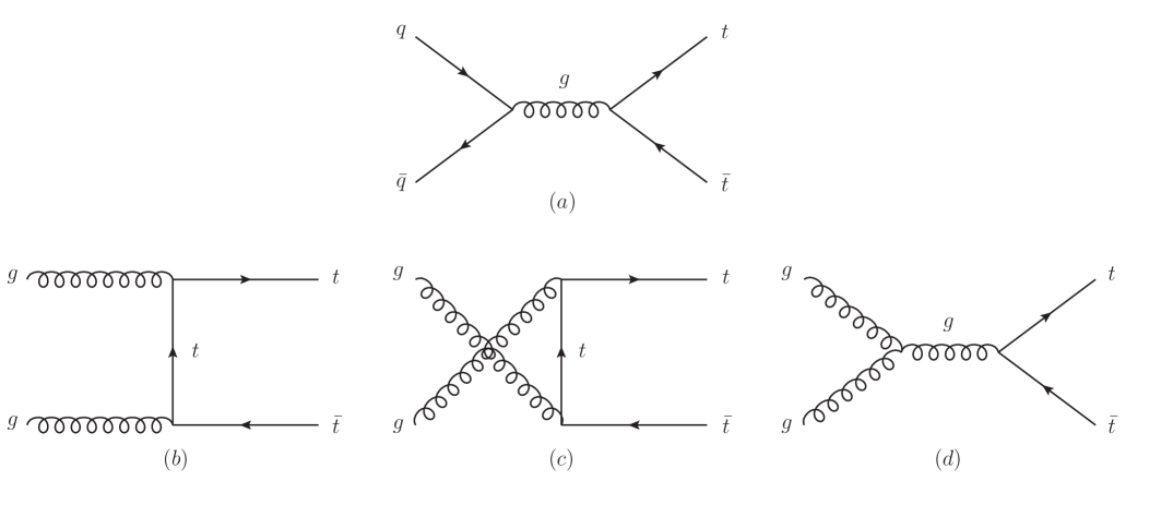
At the tree-level, the Feynman diagrams of the process $pp\to t\bar{t}$ are shown in Fig.1. The complete one-loop QCD corrections to the process $pp\to t\bar{t}$ can be generally divided into several parts: self-energies, vertex corrections, boxes and their relevant counter terms. If the amplitudes are performed at the order $\mathcal{O}(\alpha_{s}^{3})$, we find that the new particles in the LHT model only can contribute to the self-energies and the relevant counter terms, which means that there are only the LHT QCD one-loop virtual corrections to the process $pp\to t\bar{t}$. The relevant Feynman diagrams for the subprocesses $gg\to t\bar{t}$ and $q\bar{q}\to t\bar{t}$ in the LHT model are depicted in Fig.2. We can see that the LHT QCD one-loop virtual corrections ($\Delta\sigma_{\text{LHT}}$) come from the fermion loops. The one-loop QCD corrected production cross section of the process $pp\to t\bar{t}$ can be obtained by

$$\sigma_{\text{tot}}=\sigma_{\text{tree}}+\Delta\sigma_{\text{LHT}}$$ (6)

In the ’t Hooft-Feynman gauge, we use the dimensional reduction method to regulate the ultraviolet (UV) divergences in the fermion loops and adopt the on-shell renormalization scheme to remove them. We list the explicit expressions of these amplitudes in Appendix. We have checked that the UV divergences in the renormalized propagator have been canceled. Due to no massless particles in the loop, there are no infrared (IR) singularities in the one-loop integrals. In our numerical calculations, we use the parton distribution function CTEQ10cteq10 with renormalization/factorization scale $\mu_{R}=\mu_{F}=m_{t}$.

Figure 1: Tree-level Feynman diagrams of the process $pp\rightarrow t\bar{t}$ in the LHT model.

Figure 2: Feynman diagrams of the one-loop QCD correction to the process $pp\rightarrow t\bar{t}$ in the LHT model.

The relevant LHT parameters are the scale $f$, the mixing parameter $x_{L}$ and the Yukawa couplings $\kappa_{i}$. For the mirror fermion masses, we get $m_{u_{H}^{i}}=m_{d_{H}^{i}}$ at $\mathcal{O}(\upsilon/f)$ and assume that the masses of the first two generations are degeneracy:

$$m_{u_{H}^{1}}=m_{u_{H}^{2}}=m_{d_{H}^{1}}=m_{d_{H}^{2}},~{}~{}~{}~{}m_{u_{H}^{3}}=m_{d_{H}^{3}}$$ (7)

Recently, both of the CMS and ATLAS collaborations reported their search results of the fermionic top partner and respectively excluded the masses regions below 557 GeV CMS-t and 656 GeVATLAS-t at 95% CL. In our numerical calculations, we consider the constraints above and scan the parameter regions: $f=500\sim 2000$GeV, $x_{L}=0.1\sim 0.9$, $\sqrt{2}\kappa_{i}=0.6\sim 3$. And we require our samples to satisfy the constraints from Refs.constraint .

We take the input parameters of the SM asparameters

$$\sin^{2}\theta_{W}=0.231,\alpha_{s}=0.1076,\alpha_{e}=1/128,~{}~{}~{}~{}~{}~{}~{}~{}$$

$$M_{Z}=91.1876\textmd{GeV},m_{t}=173.5\textmd{GeV},m_{h}=125\textmd{GeV}.$$ (8)

We will discuss the LHT QCD one-loop corrections to the (un)polarized top pair production by using the following observables:

• For the unpolarized $t\bar{t}$ production, we calculate the relative corrections for total $t\bar{t}$ production cross section($\delta\sigma/\sigma$), which is defined by:

  $$\delta\sigma/\sigma=\frac{\sigma_{tot}-\sigma_{tree}}{\sigma_{tree}}.$$ (9)

• For the polarized $t\bar{t}$ production, we calculate the spin correlation($\delta C$)top spin SM , which is defined by:

  $$C=\frac{(\sigma_{RR}+\sigma_{LL})-(\sigma_{RL}+\sigma_{LR})}{\sigma_{RR}+\sigma_{LL}+\sigma_{RL}+\sigma_{LR}},$$ (10)

  $$\delta C=\frac{C_{tot}-C_{tree}}{C_{tree}}.$$ (11)

  Here, the subindices L(R) represent left- ($\lambda_{t(\bar{t})}=-1/2$) and right-handed($\lambda_{t(\bar{t})}=+1/2$) top(antitop) quarks, respectively.

IV Numerical results and discussions

IV.1 The correction to the $t\bar{t}$ production cross section

Figure 3: The relative correction of $t\bar{t}$ production cross section $\delta\sigma/\sigma$ as the function of $f,\kappa,x_{L}$ for $\sqrt{s}=8$ TeV and $\sqrt{s}=14$ TeV, respectively.

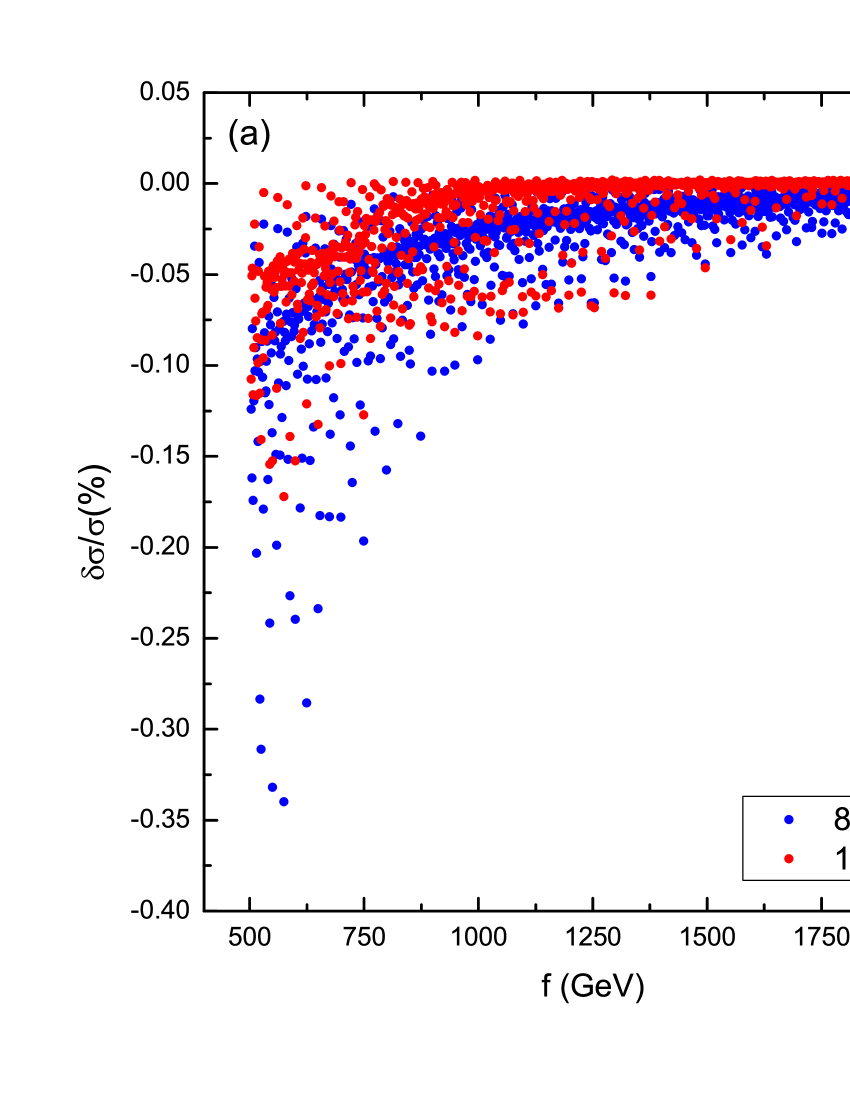
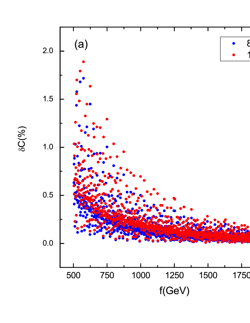
In Fig.3(a), we show the relative correction of the $t\bar{t}$ production cross section $\delta\sigma/\sigma$ as the function of the scale $f$ at the LHC with $\sqrt{s}=8,14$ TeV respectively. We can see that the maximum value of the relative correction to the $t\bar{t}$ production cross section can reach $-0.35$% for $\sqrt{s}=8$ TeV and $-0.17$% for $\sqrt{s}=14$ TeV, respectively. The results indicate that the size of the corrections and the sensitivity on these effects are larger at 8 TeV than at 14 TeV. This is because the correction of the subprocess $gg\rightarrow t\bar{t}$ is positive and the correction of the subprocess $q\bar{q}\rightarrow t\bar{t}$ is negative so that they cancel each other. Due to the main correction comes from $q\bar{q}\rightarrow t\bar{t}$, the relative correction of the $t\bar{t}$ total cross section is negative. When the center-of-mass energy $\sqrt{s}$ varies from 8 TeV to 14 TeV, the correction of the subprocess $gg\rightarrow t\bar{t}$ increases quickly so that the cancel between this two subprocesses become stronger. Besides, when the scale $f$ increases, the relative corrections $\delta\sigma/\sigma$ become small, which indicates that the LHT QCD one-loop effects on $t\bar{t}$ production cross section will decouple at the high scale $f$.

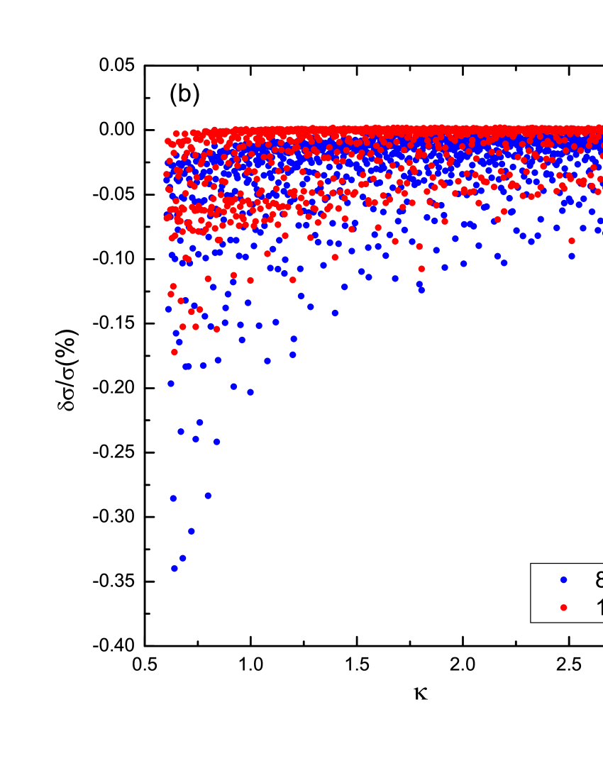
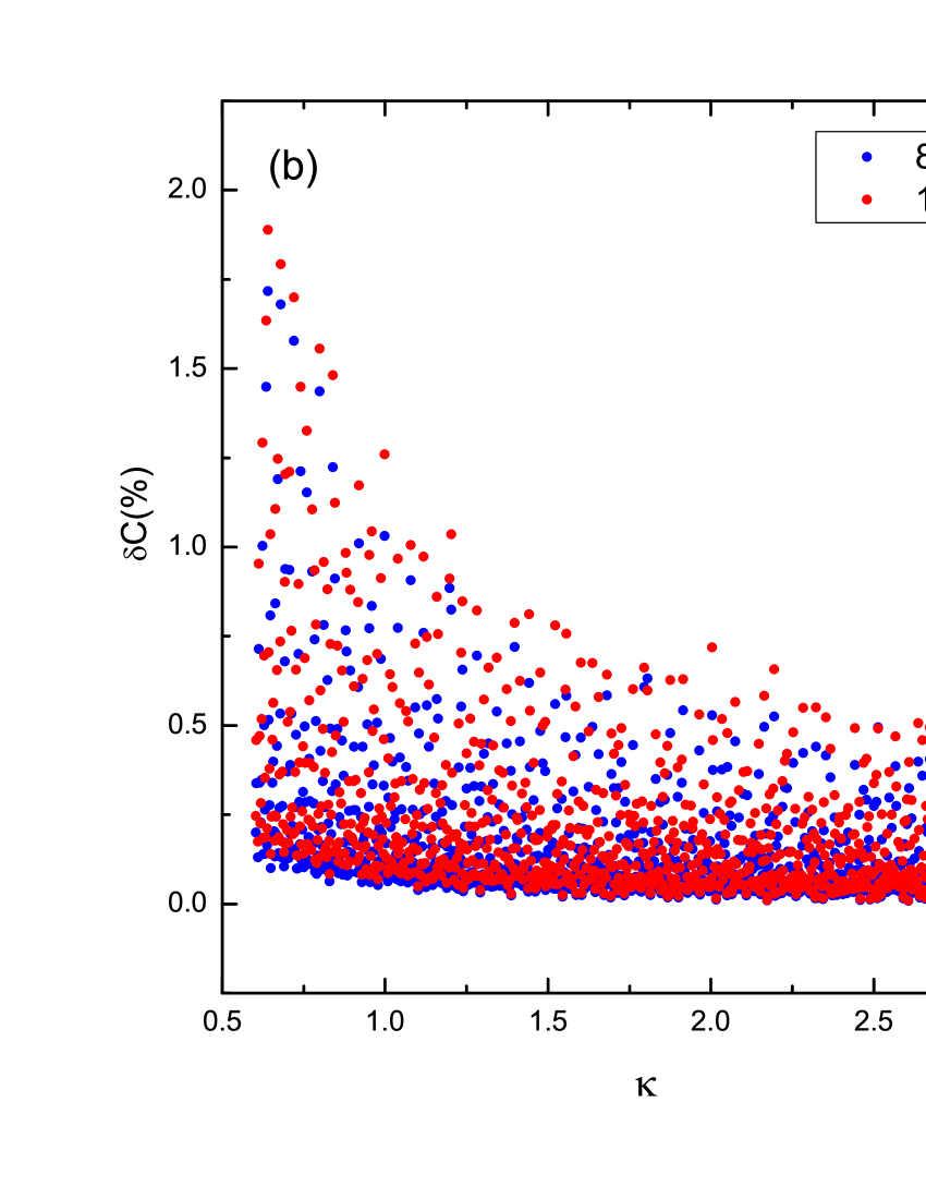
In Fig.3(b), we show the relative correction of the $t\bar{t}$ production cross section $\delta\sigma/\sigma$ as the function of the Yukawa couplings $\kappa$ at the LHC with $\sqrt{s}=8,14$ TeV respectively. We can see that the relative corrections $\delta\sigma/\sigma$ decrease with the Yukawa couplings $\kappa$ increasing, which indicates that the LHT QCD one-loop effects on $t\bar{t}$ production cross section also decouple at the heavy mirror quark masses.

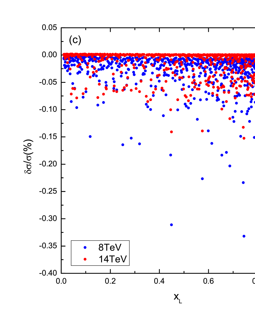
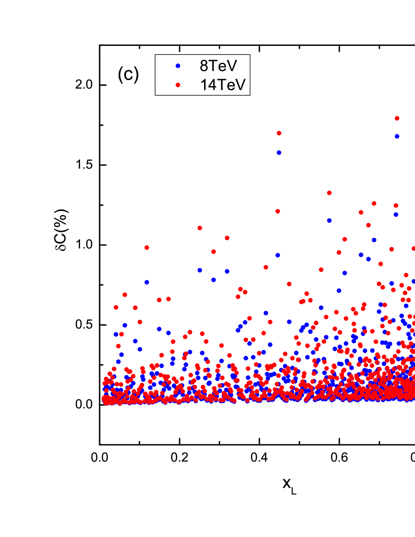
In Fig.3(c), we show the relative correction of the $t\bar{t}$ production cross section $\delta\sigma/\sigma$ as the function of the mixing parameter $x_{L}$ at the LHC with $\sqrt{s}=8,14$ TeV respectively. The distribution behaviors of the samples can be explained as follows. According to the Eqs.(4, 5), we can see that the heavy top quark $T^{+}$ and $T^{-}$ masses have a strong dependence on the mixing parameter $x_{L}$. When $x_{L}\to 0$, the masses of $T^{+}$ and $T^{-}$ will become heavy and their contribution become very small. When $x_{L}\to 1$, the masses of $T^{+}$ will become heavy while the masses of $T^{-}$ will become light. As a result, the effect of $T^{-}$ will still reside in the $t\bar{t}$ production.

IV.2 The correction to the $t\bar{t}$ spin correlation

Figure 4: The relative correction of the $t\bar{t}$ spin correlation $\delta C$ as the function of $f,\kappa,x_{L}$ for $\sqrt{s}=8$ TeV and $\sqrt{s}=14$ TeV, respectively.

Recently, the CMS collaboration reported their measurement of the $t\bar{t}$ spin correlation coefficient $C=0.24\pm 0.02(stat.)\pm 0.08(syst.)$ in the helicity basisdcLHC2 , which is agree with the SM predictions. In Fig.4, we show the relative correction of the $t\bar{t}$ spin correlation $\delta C$ as the function of $f,\kappa,x_{L}$ for the LHC with $\sqrt{s}=8,14$ TeV, respectively. We can see that the behaviors of $\delta C$ versus $f,\kappa,x_{L}$ are similar to those of the relative correction $\delta\sigma/\sigma$. The maximum value of $\delta C$ can reach about $1.7\%$ for $\sqrt{s}=8$ TeV and $2\%$ for $\sqrt{s}=14$ TeV, which may be detected at the LHCdcLHC1 .

V summary

In this paper, we studied the one-loop $\mathcal{O}(\alpha_{s}^{3})$ QCD corrections to $t\bar{t}$ production in the LHT model at the LHC for $\sqrt{s}=8,14$ TeV. We presented the numerical results for the relative correction to $t\bar{t}$ production cross section and $t\bar{t}$ spin correlation at the LHC. The relative correction of the $t\bar{t}$ production cross section is negative and only can reach $-0.35\%$. The relative correction of the $t\bar{t}$ spin correlation $\delta C$ can reach about $1.7\%$ for $\sqrt{s}=8$ TeV and $2\%$ for $\sqrt{s}=14$ TeV, which may be a potential probe to detect the LHT effects at the LHC.

Acknowledgments

This work is supported by the National Natural Science Foundation of China under grant Nos.11347140, 11305049, 11405047 and the China Postdoctoral Science Foundation under grant No. 2014M561987.

Appendix: The explicit expressions of the renormalized gluon propagator renormalization

They can be represented in form of 1-point and 2-point standard functions $A,B_{0},B_{1}$. Here $p_{t}$ and $p^{\prime}_{t}$ denote the momenta of the top and antitop respectively, and they are assumed to be outgoing.

Renormalization gluon propagator

$$-i\hat{\Sigma}_{\mu\nu}(k)=-i\Sigma_{\mu\nu}(k)+(-i\delta\Sigma_{\mu\nu}(k))$$

where

$$\Sigma_{\mu\nu}(k)=g_{\mu\nu}\Sigma_{T}(k)+k_{\mu}k_{\nu}\Sigma_{L}(k)$$

$$\delta\Sigma^{gg}_{\mu\nu}(k)=g_{\mu\nu}[\delta Z_{gg}k^{2}]$$

$$\delta Z_{gg}=-\frac{\partial\Sigma^{gg}_{T}(k^{2})}{\partial k^{2}}|_{k^{2}=0}$$

$$\hat{\Sigma}^{gg}_{\mu\nu}=\hat{\Sigma}^{gg}_{\mu\nu}(u_{H})+\hat{\Sigma}^{gg}_{\mu\nu}(d_{H})+\hat{\Sigma}^{gg}_{\mu\nu}(T^{\pm})$$

$$-i\hat{\Sigma}_{\mu\nu}^{gg}(k)=\frac{-4ig_{s}^{2}g_{\mu\nu}T_{\alpha\beta}^{a}T_{\beta\alpha}^{b}}{16\pi^{2}}$$

$$\{[-\frac{2}{3}A_{0}+\frac{2}{3}m^{2}_{T^{-}}B_{0}-\frac{2}{3}k^{2}B_{1}(k,m_{T^{-}},m_{T^{-}})+\frac{2}{3}m^{2}_{T^{-}}-\frac{k^{2}}{9}]$$

$$+[-\frac{2}{3}A_{0}+\frac{2}{3}m^{2}_{T^{+}}B_{0}-\frac{2}{3}k^{2}B_{1}(k,m_{T^{+}},m_{T^{+}})+\frac{2}{3}m^{2}_{T^{+}}-\frac{k^{2}}{9}]$$

$$+[-\frac{2}{3}A_{0}+\frac{2}{3}m^{2}_{u_{H}}B_{0}-\frac{2}{3}k^{2}B_{1}(k,m_{u_{H}},m_{u_{H}})+\frac{2}{3}m^{2}_{u_{H}}-\frac{k^{2}}{9}]$$

$$+[-\frac{2}{3}A_{0}+\frac{2}{3}m^{2}_{d_{H}}B_{0}-\frac{2}{3}k^{2}B_{1}(k,m_{d_{H}},m_{d_{H}})+\frac{2}{3}m^{2}_{d_{H}}-\frac{k^{2}}{9}]$$

$$-[\frac{2}{3}m^{2}_{T^{-}}\frac{\partial B_{0}}{\partial k^{2}}-\frac{2}{3}B_{1}(0,m_{T^{-}},m_{T^{-}})-\frac{1}{9}]k^{2}$$

$$-[\frac{2}{3}m^{2}_{T^{+}}\frac{\partial B_{0}}{\partial k^{2}}-\frac{2}{3}B_{1}(0,m_{T^{+}},m_{T^{+}})-\frac{1}{9}]k^{2}$$

$$-[\frac{2}{3}m^{2}_{u_{H}}\frac{\partial B_{0}}{\partial k^{2}}-\frac{2}{3}B_{1}(0,m_{u_{H}},m_{u_{H}})-\frac{1}{9}]k^{2}$$

$$-[\frac{2}{3}m^{2}_{d_{H}}\frac{\partial B_{0}}{\partial k^{2}}-\frac{2}{3}B_{1}(0,m_{d_{H}},m_{d_{H}})-\frac{1}{9}]k^{2}\}$$ (12)

References

- (1) CDF Collaboration, Phys. Rev. Lett. 74: 2626-2631 (1995); D Collaboration, Phys. Rev. Lett. 74: 2632-2637 (1995).
- (2) N. Arkani-Hamed, A. G. Cohen, and H. Georgi, Phys. Lett. B 513: 232 (2001); N. Arkani-Hamed, et al., JHEP 0208: 020 (2002); JHEP 0208: 021 (2002); I. Low, W. Skiba, and D. Smith, Phys. Rev. D 66: 072001 (2002); D. E. Kaplan and M. Schmaltz, JHEP 0310: 039 (2003).
- (3) N. Arkani-Hamed, A. G. Cohen, E. Katz, and A. E. Nelson, JHEP 0207: 034 (2002); S. Chang, JHEP 0312: 057 (2003); T. Han, H. E. Logan, B. McElrath, and L. T. Wang, Phys. Rev. D 67: 095004 (2003); M. Schmaltz and D. Tucker-smith, Ann. Rev. Nucl. Part. Sci. 55: 229 (2005).
- (4) C. Csaki, J. Hubisz, G.D. Kribs, P. Meade, and J. Terning, Phys. Rev. D 67: 115002 (2003); Phys. Rev. D 68: 035009 (2003); J. L. Hewett, F. J. Petriello, and T. G. Rizzo, JHEP 0310: 062 (2003); M. C. Chen and S. Dawson, Phys. Rev. D 70: 015003 (2004); M. C. Chen, et al., Mod. Phys. Lett. A 21: 621 (2006); W. Kilian, J. Reuter, Phys. Rev. D 70: 015004 (2004).
- (5) H. C. Cheng and I. Low, JHEP 0309: 051 (2003); JHEP 0408: 061 (2004); I. Low, JHEP 0410: 067 (2004); J. Hubisz and P. Meade, Phys. Rev. D 71: 035016 (2005).
- (6) G. Aad et al. (Atlas Collaboration), Eur. Phys. J. C 71: 1577 (2011); S. Chatrchyan et al. (CMS Collaboration), Eur. Phys. J. C 71: 1721 (2011); S. Chatrchyan et al. (CMS Collaboration), JHEP 1107: 049 (2011); G. Aad et al. (ATLAS Collaboration), JHEP 1205: 059 (2012); S. Chatrchyan et al. (CMS Collaboration), Phys. Rev. D 85: 112007 (2012); G. Aad et al. (ATLAS Collaboration) (2012), [arXiv:1205.2067].
- (7) B. F. Yang and N. Liu, Eur. Phys. J. C 73: 2570 (2013).
- (8) J. Cao, L. Wang, L. Wu, J. M. Yang, Phys. Rev. D 84: 074001 (2011); J. Cao, L. Wu, J. M. Yang, Phys. Rev. D 83: 034024 (2011); J. Cao, Z. Heng, L. Wu, J. M. Yang, Phys. Rev. D 81:014016 (2010).
- (9) H. L. Lai, M. Guzzi, J. Huston, Z. Li, P. M. Nadolsky, J. Pumplin, C. P. Yuan, Phys. Rev. D 82: 074024 (2010).
- (10) CMS Collaboration, Phys. Lett. B 716: 103 (2012).
- (11) ATLAS Collaboration, Phys. Lett. B 718: 1284-1302 (2013).
- (12) J. Hubisz, P. Meade, A. Noble, and M. Perelstein, J. High Energy Phys. 0601: 135 (2006); A. Belyaev, C.-R. Chen, K. Tobe, and C. P. Yuan, Phys. Rev. D 74: 115020 (2006); Q.-H. Cao and C.-R. Chen, Phys. Rev. D 76: 075007 (2007); J. Reuter, M. Tonini, JHEP 0213: 077 (2013); X. F. Han, L. Wang, J. M. Yang, J. Y. Zhu, Phys. Rev. D 87: 055004 (2013); J. Reuter, M. Tonini, M. de Vries, arXiv:1307.5010 [hep-ph], arXiv:1310.2918 [hep-ph]; C. C. Han, A. Kobakhidze, N. Liu, L. Wu, B. F. Yang, Nucl. Phys. B 890: 388-399 (2014).
- (13) J. Beringer et al., (Particle Data Group), Phys. Rev. D 86: 010001 (2012); G. Aad et al. [ATLAS Collaboration], Phys. Lett. B 716:1-29 (2012); S. Chatrchyan et al. [CMS Collaboration], CMS-HIG-12-028, arXiv:1207.7235.
- (14) J. H. Kuhn, Nucl. Phys. B 237: 77 (1984); V. D. Barger, J. Ohnemus and R. J. N. Phillips, Int. J. Mod. Phys. A 4: 617 (1989); G. Mahlon and S. J. Parke, Phys. Lett. B 411: 173 (1997); Phys. Rev. D 53: 4886 (1996); Phys. Rev. D 81: 074024 (2010); T. Stelzer and S. Willenbrock, Phys. Lett. B 374: 169 (1996); W. Bernreuther, A. Brandenburg, Z. G. Si, P. Uwer, Phys. Rev. Lett. 87: 242002 (2001); W. Bernreuther and Z. G. Si, Nucl. Phys. B 837: 90 (2010); G. Mahlon, arXiv:1007.1716 [hep-ph].
- (15) CMS Collaboration, CMS-PAS-TOP-12-004; ATLAS Collaboration, ATLAS-CONF-2013-101.
- (16) F. Hubaut, et al., Eur. Phys. J. C 44: 13 (2005).
- (17) W. F. L. Hollik, Fortschr. Phys. 38: 165-260(1990); A. Denner, Fortschr. Phys.41: 307-420 (1993).