Blended Numerical Schemes for the Advection Equation
and Conservation Laws

Simone Cacace Dipartimento di Matematica, Sapienza – Università di Roma, Rome, Italy (cacace@mat.uniroma1.it) Emiliano Cristiani Istituto per le Applicazioni del Calcolo “M. Picone”, Consiglio Nazionale delle Ricerche, Rome, Italy (e.cristiani@iac.cnr.it)  and  Roberto Ferretti Dipartimento di Matematica e Fisica, Università Roma Tre, Rome, Italy (ferretti@mat.uniroma3.it)
(Date: May 2016)
Abstract.

In this paper we propose a method to couple two or more explicit numerical schemes approximating the same time-dependent PDE, aiming at creating new schemes which inherit advantages of the original ones. We consider both advection equations and nonlinear conservation laws. By coupling a macroscopic (Eulerian) scheme with a microscopic (Lagrangian) scheme, we get a new kind of multiscale numerical method.

Key words and phrases:
multiscale numerical schemes, hyperbolic problems, conservation laws, advection equation, coupled algorithms, theta methods, WENO schemes, filtered schemes, particle level-set method, smoothed-particle hydrodynamics method, particle-in-cell method.
2010 Mathematics Subject Classification:
65M12, 65M99
This work has been partially supported by the INdAM-GNCS 2015 project “Metodi numerici semi-impliciti e semi-lagrangiani per sistemi iperbolici di leggi di bilancio”

1. Introduction

In this paper we propose and analyse a method to couple two or more numerical schemes which approximate the same time-dependent PDE. The result is a new scheme which inherits advantages (and drawbacks) of the original ones. In what follows, we will discuss how the combination might allow to improve each of the schemes, and try to derive practical coupling strategies. Roughly speaking, we combine the existing schemes by a convex combination in such a way that each scheme is influenced by the others. In the end, we get as many approximate solutions as the number of the considered schemes, but all of them are modified by the combination. In the basic version of the algorithm the coupling is performed everywhere and at any time. Nevertheless, local (in space or in time) couplings are also possible.

For illustrative purposes, we focus on the coupling of two schemes only. We consider both the case of two macroscopic (Eulerian) schemes and, more interesting, the case of a microscopic (Lagrangian, particle-based) scheme blended with a macroscopic scheme. In the latter case we get a new kind of multiscale numerical method. As a test problem, we consider the following advection equation in conservative form

{ut(x,t)+(A(x)u(x,t))x=0,xd,t>0,u(x,0)=u¯(x),xd,casessubscript𝑢𝑡𝑥𝑡subscript𝐴𝑥𝑢𝑥𝑡𝑥0formulae-sequence𝑥superscript𝑑𝑡0𝑢𝑥0¯𝑢𝑥𝑥superscript𝑑\left\{\begin{array}[]{ll}u_{t}(x,t)+(A(x)\ u(x,t))_{x}=0,&x\in\mathbb{R}^{d},\quad t>0,\\[5.69054pt] u(x,0)=\bar{u}(x),&x\in\mathbb{R}^{d},\end{array}\right. (1)

where u¯:d:¯𝑢superscript𝑑\bar{u}:\mathbb{R}^{d}\to\mathbb{R} is the initial datum and A:dd:𝐴superscript𝑑superscript𝑑A:\mathbb{R}^{d}\to\mathbb{R}^{d} is a bounded and Lipschitz continuous vector field. This equation describes the transport of a certain amount of mass in dsuperscript𝑑\mathbb{R}^{d}, drifted with velocity A𝐴A. The function u𝑢u represents the density of such a mass, so that the mass in any set Ed𝐸superscript𝑑E\subseteq\mathbb{R}^{d} at any time t𝑡t is given by

(E,t)=Eu(x,t)𝑑x.𝐸𝑡subscript𝐸𝑢𝑥𝑡differential-d𝑥\mathcal{M}(E,t)=\int_{E}u(x,t)\ dx.

In order to introduce a multiscale framework, it is useful to recast the problem at microscopic scale. Denoting by 𝒫d𝒫superscript𝑑\mathcal{P}\in\mathbb{R}^{d} the position of a generic mass particle, the Lagrangian counterpart of (1) is the ODE

𝒫˙=A(𝒫).˙𝒫𝐴𝒫\dot{\mathcal{P}}=A(\mathcal{P}). (2)

with suitable initial condition 𝒫(0)𝒫0\mathcal{P}(0).

The extension to the one-dimensional nonlinear conservation law

{ut(x,t)+f(u(x,t))x=0,x,t>0,u(x,0)=u¯(x),x,casessubscript𝑢𝑡𝑥𝑡𝑓subscript𝑢𝑥𝑡𝑥0formulae-sequence𝑥𝑡0𝑢𝑥0¯𝑢𝑥𝑥\left\{\begin{array}[]{ll}u_{t}(x,t)+f(u(x,t))_{x}=0,&x\in\mathbb{R},\quad t>0,\\[5.69054pt] u(x,0)=\bar{u}(x),&x\in\mathbb{R},\end{array}\right. (3)

will be also discussed.

The coupling idea investigated in this paper can be pursued whenever one has at his disposal two or more numerical schemes with complementary advantages and drawbacks, resulting in a blended scheme which shows a combination of these features. The idea is mainly inspired by the multiscale technique introduced in [4], which can be applied whenever one has two equations modeling the same physical phenomenon at different scales, and the velocity field explicitly appears in both equations. The blend is obtained by a convex combination of the two velocity fields, an then both the macroscopic density and the microscopic particles are transported by means of the new common multiscale velocity field, which, in turn, depends on both density and positions of the particles. Along the same line, the paper [3] blends the Brownian motion with the heat equation. Note that in these papers the goal is to improve the description of some physical phenomenon, by catching at large scale some effects ultimately triggered by small scale features, otherwise invisible. Conversely, in the present paper we blend directly the solutions of the schemes rather than the velocity fields, with the goal of improving the quality of the numerical approximation.

Relevant literature

The literature about numerical schemes for the advection equation, including multiscale numerical methods, is huge and a complete review of it is out of the scope of the paper. We will refer the interested reader to the book [13] for an introduction to the equations (1) and (3), and the basic Eulerian numerical schemes to solve them. We also mention the book [5] for a survey on the best known techniques to couple microscopic and macroscopic descriptions of physical phenomena. In the following we only discuss the schemes that can be put in relation with the one proposed in this paper.

  • The proposed scheme follows the same philosophy of Crank-Nicolson method and θ𝜃\theta-methods in general. However, there are two important differences: first, our method is explicit and combines two explicit schemes, while θ𝜃\theta-methods always combine the explicit and the implicit version of the same scheme. Second, our method has two free parameters instead of one.

  • Filtered (hybrid) schemes [9, 8, 17] suitably combine a monotone scheme with a high-order scheme, in order to get a high-order approximation minimizing spurious oscillations. In this case the coupling is restricted to Eulerian schemes.

  • The Particle-in-Cell scheme [1], often used in plasma physics, combines a Lagrangian scheme with an Eulerian grid. Roughly speaking, Lagrangian particles are independently tracked, but an underlying grid is used to recover averaged quantities. At each time step, those quantities are used for additional computations which finally give the force acting on each particle. Then the procedure is repeated for the next time step.

  • The Particle Level-Set (PLS) method [6] is a modification of the standard level-set method [18] for interfaces tracking, introduced to efficiently reduce the numerical diffusion appearing at regions of the evolving front with high curvature. Lagrangian markers are posed in a neighborhood of the interested region, and moved independently by means of a high-order ODE solver, according to the characteristic flow of the level-set equation. Whenever a particle escapes from the considered neighbourhood, it means that level-set function describing the front starts to be smeared by the diffusion. Escaped particles are then employed to recover the mass loss, i.e., to locally reinitialize the level-set function.

  • The Smoothed-Particle-Hydrodynamics (SPH) method [10, 15] (see also the Godunov-SPH [19, 12]), is an efficient computational method proposed to give some regularity to a purely Lagrangian description of a phenomenon. This is done introducing suitable convolution kernels with compact supports and thinking each Lagrangian marker as a time-dependent Dirac measure. It follows that physical macroscopic quantities of interest can be obtained by simply summing the contribution of the sole particles within the cut-off radius of the kernel. Moreover, the spatial derivative of a quantity is easily computed by linearity using the gradient of the kernel.

Finally, let us also mention the classical (W)ENO schemes [2, 11, 14, 20] (see also [7, Ch. 3]), which provide high-order accuracy of the numerical solution and can be profitably used as main ingredients of the proposed scheme.

Paper organization

In Section 2 we introduce the blended scheme for equations (1) and (3), while in Section 3 we study its theoretical properties. In Section 4 we compute the modified equation and we focus on some particular cases. In Section 5 we present several numerical tests in order to enlighten the features of our approach. Finally, we sketch some conclusions and perspectives.

2. Blended numerical scheme

To avoid cumbersome notations, let us assume d=1𝑑1d=1, results being easily generalized to any dimension. In addition, let us consider the coupling of only two numerical schemes. Let ΩT:=Ω×[0,T]assignsuperscriptΩ𝑇Ω0𝑇\Omega^{T}:=\Omega\times[0,T] be the domain in which the solution will be computed, with ΩΩ\Omega\subset\mathbb{R} a bounded domain and T>0𝑇0T>0 the final time. Let us introduce a structured grid 𝒢𝒢\mathcal{G} in ΩTsuperscriptΩ𝑇\Omega^{T} and denote by {(xi,tn)}subscript𝑥𝑖superscript𝑡𝑛\{(x_{i},t^{n})\}, i=0,,NC1,n=0,,NT1formulae-sequence𝑖0subscript𝑁𝐶1𝑛0subscript𝑁𝑇1i=0,\ldots,N_{C}-1,\ n=0,\ldots,N_{T}-1 the grid nodes, by NCsubscript𝑁𝐶N_{C}, NTsubscript𝑁𝑇N_{T}, respectively, the number of space and time nodes, and by ΔxΔ𝑥\Delta x, ΔtΔ𝑡\Delta t, respectively, the space and time discretization steps. The space grid cell is Ci=[xiΔx2,xi+Δx2)subscript𝐶𝑖subscript𝑥𝑖Δ𝑥2subscript𝑥𝑖Δ𝑥2C_{i}=\big{[}x_{i}-\frac{\Delta x}{2},x_{i}+\frac{\Delta x}{2}\big{)}.

2.1. General idea

Let us define the projection on the grid of the exact solution u𝑢u of (1)

Uin:=1ΔxCiu(x,tn)𝑑x,i=0,,NC1,n=0,,NT1,formulae-sequenceassignsuperscriptsubscript𝑈𝑖𝑛1Δ𝑥subscriptsubscript𝐶𝑖𝑢𝑥superscript𝑡𝑛differential-d𝑥formulae-sequence𝑖0subscript𝑁𝐶1𝑛0subscript𝑁𝑇1U_{i}^{n}:=\frac{1}{\Delta x}\int_{C_{i}}u(x,t^{n})dx,\qquad i=0,\ldots,N_{C}-1,\qquad n=0,\ldots,N_{T}-1, (4)

and in particular the discrete initial condition

Ui0=1ΔxCiu¯(x)𝑑x,i=0,,NC1.formulae-sequencesuperscriptsubscript𝑈𝑖01Δ𝑥subscriptsubscript𝐶𝑖¯𝑢𝑥differential-d𝑥𝑖0subscript𝑁𝐶1U_{i}^{0}=\frac{1}{\Delta x}\int_{C_{i}}\bar{u}(x)dx,\qquad i=0,\ldots,N_{C}-1. (5)

Let us also denote respectively by {𝒲in}i,nsubscriptsuperscriptsubscript𝒲𝑖𝑛𝑖𝑛\{\mathcal{W}_{i}^{n}\}_{i,n}, {𝒱in}i,nsubscriptsuperscriptsubscript𝒱𝑖𝑛𝑖𝑛\{\mathcal{V}_{i}^{n}\}_{i,n} two discrete solutions to (1) at (xi,tn)subscript𝑥𝑖superscript𝑡𝑛(x_{i},t^{n}), obtained by two (given) explicit-in-time numerical schemes of the form

{𝒲n+1=𝒮1[𝒲n]𝒲0=U0,{𝒱n+1=𝒮2[𝒱n]𝒱0=U0,n=0,,NT1,formulae-sequencecasessuperscript𝒲𝑛1subscript𝒮1delimited-[]superscript𝒲𝑛missing-subexpressionsuperscript𝒲0superscript𝑈0missing-subexpressioncasessuperscript𝒱𝑛1subscript𝒮2delimited-[]superscript𝒱𝑛missing-subexpressionsuperscript𝒱0superscript𝑈0missing-subexpression𝑛0subscript𝑁𝑇1\left\{\begin{array}[]{ll}\mathcal{W}^{n+1}=\mathcal{S}_{1}[\mathcal{W}^{n}]\\[5.69054pt] \mathcal{W}^{0}=U^{0}\end{array}\right.,\qquad\left\{\begin{array}[]{ll}\mathcal{V}^{n+1}=\mathcal{S}_{2}[\mathcal{V}^{n}]\\[5.69054pt] \mathcal{V}^{0}=U^{0}\end{array}\right.,\qquad n=0,\ldots,N_{T}-1, (6)

where 𝒮1,𝒮2:NCNC:subscript𝒮1subscript𝒮2superscriptsubscript𝑁𝐶superscriptsubscript𝑁𝐶\mathcal{S}_{1},\mathcal{S}_{2}:\mathbb{R}^{N_{C}}\to\mathbb{R}^{N_{C}}, 𝒲n:=(𝒲0n,,𝒲NC1n)assignsuperscript𝒲𝑛superscriptsubscript𝒲0𝑛superscriptsubscript𝒲subscript𝑁𝐶1𝑛\mathcal{W}^{n}:=(\mathcal{W}_{0}^{n},\ldots,\mathcal{W}_{N_{C}-1}^{n}) and 𝒱n:=(𝒱0n,,𝒱NC1n)assignsuperscript𝒱𝑛superscriptsubscript𝒱0𝑛superscriptsubscript𝒱subscript𝑁𝐶1𝑛\mathcal{V}^{n}:=(\mathcal{V}_{0}^{n},\ldots,\mathcal{V}_{N_{C}-1}^{n}). The treatment of boundary conditions is included in the definitions of the 𝒮isubscript𝒮𝑖\mathcal{S}_{i}’s.

We introduce now the blended scheme defining the two new discrete solutions {Win}i,nsubscriptsuperscriptsubscript𝑊𝑖𝑛𝑖𝑛\{W_{i}^{n}\}_{i,n} and {Vin}i,nsubscriptsuperscriptsubscript𝑉𝑖𝑛𝑖𝑛\{V_{i}^{n}\}_{i,n} to (1), with Wn:=(W0n,,WNC1n)assignsuperscript𝑊𝑛superscriptsubscript𝑊0𝑛superscriptsubscript𝑊subscript𝑁𝐶1𝑛W^{n}:=(W_{0}^{n},\ldots,W_{N_{C}-1}^{n}) and Vn:=(V0n,,VNC1n)assignsuperscript𝑉𝑛superscriptsubscript𝑉0𝑛superscriptsubscript𝑉subscript𝑁𝐶1𝑛V^{n}:=(V_{0}^{n},\ldots,V_{N_{C}-1}^{n}), by coupling 𝒮1subscript𝒮1\mathcal{S}_{1} and 𝒮2subscript𝒮2\mathcal{S}_{2} as follows

{Wn+1=λ𝒮1[Wn]+(1λ)𝒮2[Vn],Vn+1=(1μ)𝒮1[Wn]+μ𝒮2[Vn],n=0,,NT1formulae-sequencecasessuperscript𝑊𝑛1𝜆subscript𝒮1delimited-[]superscript𝑊𝑛1𝜆subscript𝒮2delimited-[]superscript𝑉𝑛superscript𝑉𝑛11𝜇subscript𝒮1delimited-[]superscript𝑊𝑛𝜇subscript𝒮2delimited-[]superscript𝑉𝑛𝑛0subscript𝑁𝑇1\boxed{\left\{\begin{array}[]{l}W^{n+1}=\lambda\mathcal{S}_{1}[W^{n}]+(1-\lambda)\mathcal{S}_{2}[V^{n}],\\[8.53581pt] V^{n+1}=(1-\mu)\mathcal{S}_{1}[W^{n}]+\mu\mathcal{S}_{2}[V^{n}],\end{array}\right.\qquad n=0,\ldots,N_{T}-1} (BS)

for some λ,μ[0,1]𝜆𝜇01\lambda,\mu\in[0,1] and initial conditions W0=V0=U0superscript𝑊0superscript𝑉0superscript𝑈0W^{0}=V^{0}=U^{0} as defined in (5). The coupling parameters λ,μ𝜆𝜇\lambda,\mu manage the convex combination between the schemes. Some remarks are in order:

  1. (i)

    if (λ,μ)(1,1)𝜆𝜇11(\lambda,\mu)\neq(1,1) the coupling occurs at each time step, hence we do not get just a trivial interpolation between the two independent numerical approximations. On the contrary, it is quite hard to say which behavior will be actually observed in the end. Moreover, there arises a natural question about which couple (λ,μ)superscript𝜆superscript𝜇(\lambda^{*},\mu^{*}) would lead to the best result. We will try to give a partial answer to this question;

  2. (ii)

    if (λ,μ)=(1,1)𝜆𝜇11(\lambda,\mu)=(1,1), the two schemes evolve independently and Wn𝒲nsuperscript𝑊𝑛superscript𝒲𝑛W^{n}\equiv\mathcal{W}^{n}, Vn𝒱nsuperscript𝑉𝑛superscript𝒱𝑛V^{n}\equiv\mathcal{V}^{n};

  3. (iii)

    if either λ=1𝜆1\lambda=1 or μ=1𝜇1\mu=1, the blend is one-way and only one solution is affected by the other;

  4. (iv)

    if (λ,μ)=(0,0)𝜆𝜇00(\lambda,\mu)=(0,0) the new scheme alternates the two original schemes at every time step, starting from 𝒮2subscript𝒮2\mathcal{S}_{2} in the case of Wnsuperscript𝑊𝑛W^{n} and 𝒮1subscript𝒮1\mathcal{S}_{1} in the case of Vnsuperscript𝑉𝑛V^{n};

  5. (v)

    if λ(0,1)𝜆01\lambda\in(0,1) and μ=0𝜇0\mu=0, (BS) reduces to a single two-step scheme

    W1=λ𝒮1[U0]+(1λ)𝒮2[U0]Wn+1=λ𝒮1[Wn]+(1λ)𝒮2[𝒮1[Wn1]],n1;superscript𝑊1𝜆subscript𝒮1delimited-[]superscript𝑈01𝜆subscript𝒮2delimited-[]superscript𝑈0missing-subexpressionsuperscript𝑊𝑛1𝜆subscript𝒮1delimited-[]superscript𝑊𝑛1𝜆subscript𝒮2delimited-[]subscript𝒮1delimited-[]superscript𝑊𝑛1𝑛1\begin{array}[]{ll}W^{1}=\lambda\mathcal{S}_{1}[U^{0}]+(1-\lambda)\mathcal{S}_{2}[U^{0}]&\\[8.53581pt] W^{n+1}=\lambda\mathcal{S}_{1}[W^{n}]+(1-\lambda)\mathcal{S}_{2}[\mathcal{S}_{1}[W^{n-1}]],&n\geq 1;\end{array}
  6. (vi)

    if λ=1μ𝜆1𝜇\lambda=1-\mu we have WnVnsuperscript𝑊𝑛superscript𝑉𝑛W^{n}\equiv V^{n} and (BS) reduces to a single scheme

    Wn+1=λ𝒮1[Wn]+(1λ)𝒮2[Wn],n0;formulae-sequencesuperscript𝑊𝑛1𝜆subscript𝒮1delimited-[]superscript𝑊𝑛1𝜆subscript𝒮2delimited-[]superscript𝑊𝑛𝑛0W^{n+1}=\lambda\mathcal{S}_{1}[W^{n}]+(1-\lambda)\mathcal{S}_{2}[W^{n}],\qquad n\geq 0;
  7. (vii)

    generalization to multi-blend is straightforward. If we have \mathcal{L} schemes 𝒮1,,𝒮subscript𝒮1subscript𝒮\mathcal{S}_{1},\ldots,{\mathcal{S}}_{\mathcal{L}}, the blended scheme is

    (Wn+1,(1)Wn+1,())=(λ11λ1λ1λ)(𝒮1[Wn,(1)]𝒮[Wn,()])superscript𝑊𝑛11superscript𝑊𝑛1superscriptsubscript𝜆11superscriptsubscript𝜆1superscriptsubscript𝜆1superscriptsubscript𝜆subscript𝒮1delimited-[]superscript𝑊𝑛1subscript𝒮delimited-[]superscript𝑊𝑛\left(\begin{array}[]{c}W^{n+1,(1)}\\ \vdots\\ W^{n+1,(\mathcal{L})}\end{array}\right)=\left(\begin{array}[]{ccc}\lambda_{1}^{1}&\ldots&\lambda_{\mathcal{L}}^{1}\\ \vdots&\ddots&\vdots\\ \lambda_{1}^{\mathcal{L}}&\ldots&\lambda_{\mathcal{L}}^{\mathcal{L}}\end{array}\right)\left(\begin{array}[]{c}\mathcal{S}_{1}[W^{n,(1)}]\\ \vdots\\ \mathcal{S}_{\mathcal{L}}[W^{n,(\mathcal{L})}]\end{array}\right)

    where the coupling parameters {λij}superscriptsubscript𝜆𝑖𝑗\{\lambda_{i}^{j}\} are such that j=1λji=1superscriptsubscript𝑗1superscriptsubscript𝜆𝑗𝑖1\sum_{j=1}^{\mathcal{L}}\lambda_{j}^{i}=1, for all i=1,,𝑖1i=1,\ldots,\mathcal{L};

  8. (viii)

    a more sophisticated blend could allow (λ,μ)𝜆𝜇(\lambda,\mu) to depend on space, time, and the solution itself. In this way we can construct ad hoc recipes wherever the solution shows some critical behaviour.

2.2. Multiscale coupling

In this section we transform the blended scheme (BS) in a multiscale scheme, by choosing an Eulerian approximation for 𝒮1subscript𝒮1\mathcal{S}_{1} (e.g., Upwind, Lax-Friedrichs, (W)ENO, Godunov, etc.) and a Lagrangian approximation for 𝒮2subscript𝒮2\mathcal{S}_{2}. First, we consider a number of Lagrangian particles which move in ΩΩ\Omega driven by the velocity field A𝐴A. We assume that, at the initial time t=0𝑡0t=0, we have NPsubscript𝑁PN_{\text{P}} particles. We denote the (positions of the) particles at time t𝑡t by 𝒫α(t)subscript𝒫𝛼𝑡\mathcal{P}_{\alpha}(t), for α=0,,NP1𝛼0subscript𝑁P1\alpha=0,\ldots,N_{\text{P}}-1. We also denote by NPC=NPNCsubscript𝑁PCsubscript𝑁Psubscript𝑁𝐶N_{\text{PC}}=\frac{N_{\text{P}}}{N_{C}}\in\mathbb{Q} the number of particles per cell.

Initialization

At time t=0𝑡0t=0, the particles are uniformly placed in ΩΩ\Omega, i.e.,

𝒫α(0)=x0+αΔp,α=0,,NP1,Δp=xNC1x0NP1.formulae-sequencesubscript𝒫𝛼0subscript𝑥0𝛼Δ𝑝formulae-sequence𝛼0subscript𝑁P1Δ𝑝subscript𝑥subscript𝑁𝐶1subscript𝑥0subscript𝑁P1\mathcal{P}_{\alpha}(0)=x_{0}+\alpha\Delta p,\quad\alpha=0,\ldots,N_{\text{P}}-1\,,\qquad\Delta p=\frac{x_{N_{C}-1}-x_{0}}{N_{\text{P}}-1}. (7)

Moreover, each particle is endowed with a “weight”, i.e. a portion of the mass transported by (1). Denoting by α(t)subscript𝛼𝑡\mathcal{M}_{\alpha}(t) the mass assigned to the α𝛼\alpha-th particle at time t𝑡t, we set

α(0)=u¯(𝒫α(0))ΔxNPC.subscript𝛼0¯𝑢subscript𝒫𝛼0Δ𝑥subscript𝑁PC\mathcal{M}_{\alpha}(0)=\bar{u}\big{(}\mathcal{P}_{\alpha}(0)\big{)}\frac{\Delta x}{N_{\text{PC}}}. (8)

Note that, in a purely Lagrangian framework, there is no need to consider a time-dependent mass for each particle because it remains constant during the evolution. Therefore, one can initially distribute the particles in space according to u¯¯𝑢\bar{u}, interpreting the initial condition as the probability density function of the mass. Here instead we define the mass αsubscript𝛼\mathcal{M}_{\alpha} as a time-dependent variable because of the combination with the Eulerian part of the algorithm, which will modify the masses at each time step.

Note that one can avoid to put particles in regions in which u¯=0¯𝑢0\bar{u}=0, thus saving CPU time. For simplicity, we put particles all along ΩΩ\Omega, regardless of the values of u¯¯𝑢\bar{u}.

Particles evolution

As already mentioned in the introduction, the dynamics of each particle α𝛼\alpha is given by the ODE

𝒫˙α(t)=A(𝒫α(t)).subscript˙𝒫𝛼𝑡𝐴subscript𝒫𝛼𝑡\dot{\mathcal{P}}_{\alpha}(t)=A(\mathcal{P}_{\alpha}(t)). (9)

It is then natural to solve (9) by means of an ODE solver. Focusing on one-step ODE solvers, the general algorithm has the form

{𝒫αn+1=𝒮ODE(𝒫αn),n=0,,NT1,𝒫α0=𝒫α(0),casesformulae-sequencesuperscriptsubscript𝒫𝛼𝑛1subscript𝒮ODEsuperscriptsubscript𝒫𝛼𝑛𝑛0subscript𝑁𝑇1superscriptsubscript𝒫𝛼0subscript𝒫𝛼0\left\{\begin{array}[]{l}\mathcal{P}_{\alpha}^{n+1}=\mathcal{S}_{\textup{ODE}}(\mathcal{P}_{\alpha}^{n}),\qquad n=0,\ldots,N_{T}-1,\\[5.69054pt] \mathcal{P}_{\alpha}^{0}=\mathcal{P}_{\alpha}(0),\end{array}\right. (10)

where 𝒫αn:=𝒫α(tn)assignsuperscriptsubscript𝒫𝛼𝑛subscript𝒫𝛼superscript𝑡𝑛\mathcal{P}_{\alpha}^{n}:=\mathcal{P}_{\alpha}(t^{n}).

Computation of the Lagrangian density

In order to combine the approximate Eulerian density with the Lagrangian computation we need a suitable averaging of the masses of the particles 𝒫αsubscript𝒫𝛼\mathcal{P}_{\alpha}’s, so to recover an approximate Lagrangian density. To this end we set

V^in+1:=(𝒮2[𝒫n+1,n])i=1Δxα:𝒫αn+1Ciαn.assignsubscriptsuperscript^𝑉𝑛1𝑖subscriptsubscript𝒮2superscript𝒫𝑛1superscript𝑛𝑖1Δ𝑥subscript:𝛼superscriptsubscript𝒫𝛼𝑛1subscript𝐶𝑖superscriptsubscript𝛼𝑛\widehat{V}^{n+1}_{i}:=(\mathcal{S}_{2}[\mathcal{P}^{n+1},\mathcal{M}^{n}])_{i}=\frac{1}{\Delta x}\sum_{\alpha\ \!:\ \!\mathcal{P}_{\alpha}^{n+1}\in C_{i}}\mathcal{M}_{\alpha}^{n}. (11)

where αn=α(tn)superscriptsubscript𝛼𝑛subscript𝛼superscript𝑡𝑛\mathcal{M}_{\alpha}^{n}=\mathcal{M}_{\alpha}(t^{n}). Let us explain this definition: at any time tnsuperscript𝑡𝑛t^{n} and for any cell Cisubscript𝐶𝑖C_{i}, we find the particles falling in the cell Cisubscript𝐶𝑖C_{i}, summing all their masses and dividing by the area of the cell. Note that V^n+1superscript^𝑉𝑛1\widehat{V}^{n+1} is computed by the updated positions of the particles 𝒫n+1superscript𝒫𝑛1\mathcal{P}^{n+1} and the last available values for the masses.

Blending and mass update

Given W^in+1:=(𝒮1[Wn])iassignsubscriptsuperscript^𝑊𝑛1𝑖subscriptsubscript𝒮1delimited-[]superscript𝑊𝑛𝑖\widehat{W}^{n+1}_{i}:=(\mathcal{S}_{1}[W^{n}])_{i} and V^in+1subscriptsuperscript^𝑉𝑛1𝑖\widehat{V}^{n+1}_{i} as in (11) at any space and time node, we are ready to run the scheme (BS) and compute the blended approximations W𝑊W and V𝑉V. However, modifying the Lagrangian density (from V^^𝑉\widehat{V} to V𝑉V) leaves the particles unchanged (both masses \mathcal{M} and positions 𝒫𝒫\mathcal{P}). Since the Lagrangian density is computed at each time step by means of \mathcal{M} and 𝒫𝒫\mathcal{P}, see (11), we are going to lose the coupling effect after every time step. To fix this, we adopt the following strategy: at every time step, we modify the masses αnsuperscriptsubscript𝛼𝑛\mathcal{M}_{\alpha}^{n} according to the modified Lagrangian density Vn+1superscript𝑉𝑛1V^{n+1}. More, precisely, we denote by ΛinsuperscriptsubscriptΛ𝑖𝑛\Lambda_{i}^{n} the number of particles falling in the cell Cisubscript𝐶𝑖C_{i} at time tnsuperscript𝑡𝑛t^{n} and update their mass by setting:

αn+1=αn+{ΔxΛin(Vin+1(𝒮2[𝒫n+1,n])i),if Λin>00,otherwise.subscriptsuperscript𝑛1𝛼subscriptsuperscript𝑛𝛼casesΔ𝑥superscriptsubscriptΛ𝑖𝑛superscriptsubscript𝑉𝑖𝑛1subscriptsubscript𝒮2superscript𝒫𝑛1superscript𝑛𝑖if superscriptsubscriptΛ𝑖𝑛00otherwise.\mathcal{M}^{n+1}_{\alpha}=\mathcal{M}^{n}_{\alpha}+\left\{\begin{array}[]{ll}\displaystyle\frac{\Delta x}{\Lambda_{i}^{n}}\Big{(}V_{i}^{n+1}-(\mathcal{S}_{2}[\mathcal{P}^{n+1},\mathcal{M}^{n}])_{i}\Big{)},&\text{if }\Lambda_{i}^{n}>0\\[11.38109pt] 0,&\text{otherwise.}\end{array}\right. (12)

Obviously, since the Lagrangian density is constant on each cell, all the particles falling in the same cell are equally affected. Note that, as opposed to the masses, the positions 𝒫αsubscript𝒫𝛼\mathcal{P}_{\alpha} are not affected by the coupling.

Final algorithm

Summarizing, the complete algorithm for one time step (Wn,Vn;𝒫n,n)superscript𝑊𝑛superscript𝑉𝑛superscript𝒫𝑛superscript𝑛(W^{n},V^{n};\mathcal{P}^{n},\mathcal{M}^{n}) \to (Wn+1,Vn+1;𝒫n+1,n+1)superscript𝑊𝑛1superscript𝑉𝑛1superscript𝒫𝑛1superscript𝑛1(W^{n+1},V^{n+1};\mathcal{P}^{n+1},\mathcal{M}^{n+1}) is the following:

  1. (1)

    Compute W^in+1=(𝒮1[Wn])isubscriptsuperscript^𝑊𝑛1𝑖subscriptsubscript𝒮1delimited-[]superscript𝑊𝑛𝑖\widehat{W}^{n+1}_{i}=(\mathcal{S}_{1}[W^{n}])_{i}.

  2. (2)

    Compute 𝒫αn+1subscriptsuperscript𝒫𝑛1𝛼\mathcal{P}^{n+1}_{\alpha} by (10) (all α𝛼\alpha’s).

  3. (3)

    Compute V^in+1=(𝒮2[𝒫n+1,n])isubscriptsuperscript^𝑉𝑛1𝑖subscriptsubscript𝒮2superscript𝒫𝑛1superscript𝑛𝑖\widehat{V}^{n+1}_{i}=(\mathcal{S}_{2}[\mathcal{P}^{n+1},\mathcal{M}^{n}])_{i} by (11) (all i𝑖i’s).

  4. (4)

    Compute Wn+1superscript𝑊𝑛1W^{n+1} and Vn+1superscript𝑉𝑛1V^{n+1} by (BS).

  5. (5)

    Compute αn+1subscriptsuperscript𝑛1𝛼\mathcal{M}^{n+1}_{\alpha} by (12) (all α𝛼\alpha’s).

{rmrk}

(Partial coupling) If μ=1𝜇1\mu=1 the algorithm simplifies since there is no need to correct the masses, see (12). {rmrk} (Parallelization) The Lagrangian part of the multiscale algorithm can be easily and efficiently parallelized on both distributed and shared memory architectures since particles do not need to communicate with each other. In particular it is not needed to find the neighboring particles of each particle (as required in, e.g., SPH method).

2.3. Extension to one-dimensional nonlinear conservation laws

In this section we show how the blended scheme can be extended to equation (3). The Eulerian-Eulerian coupling does not need any modification and then it is no further discussed. The multiscale coupling (Section 2.2) needs instead some corrections. In conservation laws, the velocity A𝐴A of the particles (not that of the characteristic curves) can be recovered from the flux f𝑓f as A(u):=f(u)uassign𝐴𝑢𝑓𝑢𝑢A(u):=\frac{f(u)}{u} (if u0𝑢0u\neq 0) and equation (9) must be replaced by

𝒫˙α(t)=A(u(𝒫α(t),t)).subscript˙𝒫𝛼𝑡𝐴𝑢subscript𝒫𝛼𝑡𝑡\dot{\mathcal{P}}_{\alpha}(t)=A\big{(}u(\mathcal{P}_{\alpha}(t),t)\big{)}.

This means that the Lagrangian scheme needs the density u𝑢u to update the positions of the particles. The blended scheme provides at each time step two approximate densities, namely Wnsuperscript𝑊𝑛W^{n} and Vnsuperscript𝑉𝑛V^{n}. Hence we solve either

𝒫˙α(tn)=A(Wjα,nn)or𝒫˙α(tn)=A(Vjα,nn),formulae-sequencesubscript˙𝒫𝛼superscript𝑡𝑛𝐴subscriptsuperscript𝑊𝑛subscript𝑗𝛼𝑛orsubscript˙𝒫𝛼superscript𝑡𝑛𝐴subscriptsuperscript𝑉𝑛subscript𝑗𝛼𝑛\dot{\mathcal{P}}_{\alpha}(t^{n})=A(W^{n}_{j_{\alpha,n}})\qquad\text{or}\qquad\dot{\mathcal{P}}_{\alpha}(t^{n})=A(V^{n}_{j_{\alpha,n}})\,, (13)

where jα,nsubscript𝑗𝛼𝑛j_{\alpha,n} is the cell where the α𝛼\alpha-th particle falls in at time tnsuperscript𝑡𝑛t^{n}. Note that, choosing Wnsuperscript𝑊𝑛W^{n}, we introduces an additional coupling: the Lagrangian scheme now depends on the Eulerian scheme even for an uncoupled evolution (λ,μ)=(1,1)𝜆𝜇11(\lambda,\mu)=(1,1).

2.4. Estimation of coupling parameters (λ,μ)𝜆𝜇(\lambda,\mu) by Richardson extrapolation

The blended scheme (BS) is actually a family of numerical schemes indexed by two coupling parameters (λ,μ)[0,1]2𝜆𝜇superscript012(\lambda,\mu)\in[0,1]^{2}. Generally speaking, we expect that only some couples lead to a solution W𝑊W or V𝑉V which is better than both solutions 𝒲𝒲\mathcal{W} and 𝒱𝒱\mathcal{V} obtained by the uncoupled schemes. The question arises how to find an advantageous couple a priori, before running the computation and without the knowledge of the exact solution. In some simple cases one can compute the optimal parameters analytically, but in general this is impossible. In order to provide a general method, we adopt the following strategy.

First of all, let us denote the solutions of the blended scheme (BS) by {Win(λ,μ)}i,nsubscriptsubscriptsuperscript𝑊𝑛𝑖𝜆𝜇𝑖𝑛\{W^{n}_{i}(\lambda,\mu)\}_{i,n} and {Vin(λ,μ)}i,nsubscriptsubscriptsuperscript𝑉𝑛𝑖𝜆𝜇𝑖𝑛\{V^{n}_{i}(\lambda,\mu)\}_{i,n} in order to make it explicit the dependence on the coupling parameters. Moreover, let us define the L1superscript𝐿1L^{1} errors at final time as

E1[W(λ,μ)]:=i|WiNT(λ,μ)UiNT|Δx,E1[V(λ,μ)]:=i|ViNT(λ,μ)UiNT|Δx,\begin{split}E^{1}[W(\lambda,\mu)]:=\sum_{i}\Big{|}W^{N_{T}}_{i}(\lambda,\mu)-U^{N_{T}}_{i}\Big{|}\Delta x,\qquad E^{1}[V(\lambda,\mu)]:=\sum_{i}\Big{|}V^{N_{T}}_{i}(\lambda,\mu)-U^{N_{T}}_{i}\Big{|}\Delta x,\end{split} (14)

and define the two optimal L1superscript𝐿1L^{1} couplings as

(λ,μ)W:=argminλ,μE1[W(λ,μ)],(λ,μ)V:=argminλ,μE1[V(λ,μ)].\begin{split}(\lambda^{*},\mu^{*})_{W}:=\arg\min_{\lambda,\mu}E^{1}[W(\lambda,\mu)],\qquad(\lambda^{*},\mu^{*})_{V}:=\arg\min_{\lambda,\mu}E^{1}[V(\lambda,\mu)].\end{split} (15)

Following the classical idea of Richardson extrapolation, we can run the blended scheme on two (coarse) grids, 𝒢superscript𝒢\mathcal{G}^{\prime} and 𝒢′′superscript𝒢′′\mathcal{G}^{\prime\prime}, thus obtaining, for each (λ,μ)𝜆𝜇(\lambda,\mu), four solutions W(λ,μ;𝒢)𝑊𝜆𝜇superscript𝒢W(\lambda,\mu;\mathcal{G}^{\prime}), V(λ,μ;𝒢)𝑉𝜆𝜇superscript𝒢V(\lambda,\mu;\mathcal{G}^{\prime}), W(λ,μ;𝒢′′)𝑊𝜆𝜇superscript𝒢′′W(\lambda,\mu;\mathcal{G}^{\prime\prime}), and V(λ,μ;𝒢′′)𝑉𝜆𝜇superscript𝒢′′V(\lambda,\mu;\mathcal{G}^{\prime\prime}). Then we define the two Richardson L1superscript𝐿1L^{1} error indicators as

δWR(λ,μ;𝒢,𝒢′′):=i𝒢|WiNT(λ,μ;𝒢)Wh(i)NT(λ,μ;𝒢′′)|Δx,δVR(λ,μ;𝒢,𝒢′′):=i𝒢|ViNT(λ,μ;𝒢)Vh(i)NT(λ,μ;𝒢′′)|Δx,formulae-sequenceassignsubscriptsuperscript𝛿𝑅𝑊𝜆𝜇superscript𝒢superscript𝒢′′subscript𝑖superscript𝒢superscriptsubscript𝑊𝑖subscript𝑁𝑇𝜆𝜇superscript𝒢superscriptsubscript𝑊𝑖subscript𝑁𝑇𝜆𝜇superscript𝒢′′Δ𝑥assignsubscriptsuperscript𝛿𝑅𝑉𝜆𝜇superscript𝒢superscript𝒢′′subscript𝑖superscript𝒢superscriptsubscript𝑉𝑖subscript𝑁𝑇𝜆𝜇superscript𝒢superscriptsubscript𝑉𝑖subscript𝑁𝑇𝜆𝜇superscript𝒢′′Δ𝑥\begin{split}\delta^{R}_{W}(\lambda,\mu;\mathcal{G}^{\prime},\mathcal{G}^{\prime\prime}):=\sum_{i\in\mathcal{G}^{\prime}}\left|W_{i}^{N_{T}}(\lambda,\mu;\mathcal{G}^{\prime})-W_{h(i)}^{N_{T}}(\lambda,\mu;\mathcal{G}^{\prime\prime})\right|\Delta x,\\ \delta^{R}_{V}(\lambda,\mu;\mathcal{G}^{\prime},\mathcal{G}^{\prime\prime}):=\sum_{i\in\mathcal{G}^{\prime}}\left|V_{i}^{N_{T}}(\lambda,\mu;\mathcal{G}^{\prime})-V_{h(i)}^{N_{T}}(\lambda,\mu;\mathcal{G}^{\prime\prime})\right|\Delta x,\end{split} (16)

where h(i)𝑖h(i) gives the best correspondence from node i𝑖i in 𝒢superscript𝒢\mathcal{G}^{\prime} to a node in 𝒢′′superscript𝒢′′\mathcal{G}^{\prime\prime}. The estimates for (λ,μ)superscript𝜆superscript𝜇(\lambda^{*},\mu^{*}) are then given by

(λR,μR)W,𝒢,𝒢′′:=argminλ,μδWR(λ,μ;𝒢,𝒢′′),(λR,μR)V,𝒢,𝒢′′:=argminλ,μδVR(λ,μ;𝒢,𝒢′′).formulae-sequenceassignsubscriptsuperscript𝜆𝑅superscript𝜇𝑅𝑊superscript𝒢superscript𝒢′′subscript𝜆𝜇subscriptsuperscript𝛿𝑅𝑊𝜆𝜇superscript𝒢superscript𝒢′′assignsubscriptsuperscript𝜆𝑅superscript𝜇𝑅𝑉superscript𝒢superscript𝒢′′subscript𝜆𝜇subscriptsuperscript𝛿𝑅𝑉𝜆𝜇superscript𝒢superscript𝒢′′\begin{split}(\lambda^{R},\mu^{R})_{W,\mathcal{G}^{\prime},\mathcal{G}^{\prime\prime}}:=\arg\min_{\lambda,\mu}\delta^{R}_{W}(\lambda,\mu;\mathcal{G}^{\prime},\mathcal{G}^{\prime\prime}),\\ (\lambda^{R},\mu^{R})_{V,\mathcal{G}^{\prime},\mathcal{G}^{\prime\prime}}:=\arg\min_{\lambda,\mu}\delta^{R}_{V}(\lambda,\mu;\mathcal{G}^{\prime},\mathcal{G}^{\prime\prime}).\end{split} (17)
{rmrk}

It is possible to avoid an exhaustive search in [0,1]2superscript012[0,1]^{2} in (17) by employing a descend method in the space (λ,μ)𝜆𝜇(\lambda,\mu) starting from some initial guess (λ0,μ0)subscript𝜆0subscript𝜇0(\lambda_{0},\mu_{0}). One can also progressively refine the grid (in the space (λ,μ)𝜆𝜇(\lambda,\mu)) around the argmin found in the previous level. {rmrk} A necessary condition for the method to work is that (λ,μ)superscript𝜆superscript𝜇(\lambda^{*},\mu^{*}) is stable with respect to the grid size. In Section 5 we will investigate this property. Moreover, we expect the method to be sufficiently fast if performed on very coarse grids, in particular much coarser than the final grid where the actual computation must be performed.

3. Theoretical analysis

We address in this section the main theoretical issues for the blended scheme solving equation (1) with d=1𝑑1d=1. Note that, rather than perform a complete convergence analysis (which apparently requires more technical subtleties), we will analyze the scheme in the two situations which seem to be more effective and that are actually used in numerical examples, i.e., the coupling of two Eulerian schemes and the use of a Lagrangian scheme to correct an Eulerian scheme in a multi-scale approach (i.e. λ[0,1)𝜆01\lambda\in[0,1) and μ=1𝜇1\mu=1).

3.1. Mass conservation

We first prove that the scheme (BS) is conservative, provided the two constitutive schemes are so. Let us use again the notation

W^in+1=(𝒮1[Wn])i,V^in+1=(𝒮2[Vn])iformulae-sequencesuperscriptsubscript^𝑊𝑖𝑛1subscriptsubscript𝒮1delimited-[]superscript𝑊𝑛𝑖superscriptsubscript^𝑉𝑖𝑛1subscriptsubscript𝒮2delimited-[]superscript𝑉𝑛𝑖\widehat{W}_{i}^{n+1}=(\mathcal{S}_{1}[W^{n}])_{i},\qquad\qquad\widehat{V}_{i}^{n+1}=(\mathcal{S}_{2}[V^{n}])_{i} (18)

for a single time step of the uncoupled schemes (with a slight abuse of notation in the case of multiscale algorithm).

{prpstn}

Assume that the solvers (18) are conservative, i.e.

iW^in+1=iWin,iV^in+1=iVin,formulae-sequencesubscript𝑖superscriptsubscript^𝑊𝑖𝑛1subscript𝑖superscriptsubscript𝑊𝑖𝑛subscript𝑖superscriptsubscript^𝑉𝑖𝑛1subscript𝑖superscriptsubscript𝑉𝑖𝑛\sum_{i}\widehat{W}_{i}^{n+1}=\sum_{i}W_{i}^{n},\qquad\sum_{i}\widehat{V}_{i}^{n+1}=\sum_{i}V_{i}^{n}, (19)

and that

iWi0=iVi0=iUi0.subscript𝑖subscriptsuperscript𝑊0𝑖subscript𝑖subscriptsuperscript𝑉0𝑖subscript𝑖subscriptsuperscript𝑈0𝑖\sum_{i}W^{0}_{i}=\sum_{i}V^{0}_{i}=\sum_{i}U^{0}_{i}. (20)

Then, the scheme (BS) is also conservative.

Proof.

By definition of the scheme (BS) and (18), we have

{iWin+1=λiW^in+1+(1λ)iV^in+1iVin+1=(1μ)iW^in+1+μiV^in+1,casessubscript𝑖superscriptsubscript𝑊𝑖𝑛1𝜆subscript𝑖superscriptsubscript^𝑊𝑖𝑛11𝜆subscript𝑖superscriptsubscript^𝑉𝑖𝑛1otherwisesubscript𝑖superscriptsubscript𝑉𝑖𝑛11𝜇subscript𝑖superscriptsubscript^𝑊𝑖𝑛1𝜇subscript𝑖superscriptsubscript^𝑉𝑖𝑛1otherwise\begin{cases}\sum_{i}W_{i}^{n+1}=\lambda\sum_{i}\widehat{W}_{i}^{n+1}+(1-\lambda)\sum_{i}\widehat{V}_{i}^{n+1}\\ \sum_{i}V_{i}^{n+1}=(1-\mu)\sum_{i}\widehat{W}_{i}^{n+1}+\mu\sum_{i}\widehat{V}_{i}^{n+1},\end{cases} (21)

so that, using the discrete conservation of both schemes (19), we have

{iWin+1=λiWin+(1λ)iViniVin+1=(1μ)iWin+μiVin,casessubscript𝑖superscriptsubscript𝑊𝑖𝑛1𝜆subscript𝑖superscriptsubscript𝑊𝑖𝑛1𝜆subscript𝑖superscriptsubscript𝑉𝑖𝑛otherwisesubscript𝑖superscriptsubscript𝑉𝑖𝑛11𝜇subscript𝑖superscriptsubscript𝑊𝑖𝑛𝜇subscript𝑖superscriptsubscript𝑉𝑖𝑛otherwise\begin{cases}\sum_{i}W_{i}^{n+1}=\lambda\sum_{i}W_{i}^{n}+(1-\lambda)\sum_{i}V_{i}^{n}\\ \sum_{i}V_{i}^{n+1}=(1-\mu)\sum_{i}W_{i}^{n}+\mu\sum_{i}V_{i}^{n},\end{cases}

which implies that

iWin+1,iVin+1[min(iWin,iVin),max(iWin,iVin)].subscript𝑖superscriptsubscript𝑊𝑖𝑛1subscript𝑖superscriptsubscript𝑉𝑖𝑛1subscript𝑖superscriptsubscript𝑊𝑖𝑛subscript𝑖superscriptsubscript𝑉𝑖𝑛subscript𝑖superscriptsubscript𝑊𝑖𝑛subscript𝑖superscriptsubscript𝑉𝑖𝑛\sum_{i}W_{i}^{n+1},\sum_{i}V_{i}^{n+1}\in\left[\min\left(\sum_{i}W_{i}^{n},\sum_{i}V_{i}^{n}\right),\ \max\left(\sum_{i}W_{i}^{n},\sum_{i}V_{i}^{n}\right)\right].

The proof is concluded by induction noting that (20) holds. ∎

{rmrk}

The previous result remains true if both parameters λ𝜆\lambda and μ𝜇\mu depend on the step index n𝑛n, but not if they depend on the cell index i𝑖i.

3.2. Coupling between two Eulerian schemes

Hereafter we will assume for simplicity that the schemes 𝒮1,𝒮2subscript𝒮1subscript𝒮2\mathcal{S}_{1},\mathcal{S}_{2} are linear, so that we can write

𝒲n+1=S1𝒲n,𝒱n+1=S2𝒱n,\mathcal{W}^{n+1}=S_{1}\mathcal{W}^{n}\quad,\qquad\mathcal{V}^{n+1}=S_{2}\mathcal{V}^{n},

where S1,S2subscript𝑆1subscript𝑆2S_{1},S_{2} are two NC×NCsubscript𝑁𝐶subscript𝑁𝐶N_{C}\times N_{C} matrices. Let us also assume that each of the schemes is stable, and in particular that they satisfy

S1p11+C1Δt,S2p21+C2Δt,\|S_{1}\|_{p_{1}}\leq 1+C_{1}\Delta t\quad,\qquad\|S_{2}\|_{p_{2}}\leq 1+C_{2}\Delta t, (22)

with constants C1,C2subscript𝐶1subscript𝐶2C_{1},C_{2} independent of ΔxΔ𝑥\Delta x and ΔtΔ𝑡\Delta t, and for some (possibly different) suitable norms pi\|\cdot\|_{p_{i}} (i=1,2)𝑖12(i=1,2) which could be required for the convergence analysis of the two schemes (e.g., \infty-norm for a monotone scheme and 222-norm for a high order scheme). We also assume to use scaled lpsuperscript𝑙𝑝l^{p} norms defined by

Up=Δx1/p(j|uj|p)1/p.subscriptnorm𝑈𝑝Δsuperscript𝑥1𝑝superscriptsubscript𝑗superscriptsubscript𝑢𝑗𝑝1𝑝\|U\|_{p}=\Delta x^{1/p}\left(\sum_{j}|u_{j}|^{p}\right)^{1/p}. (23)

Now, the scheme (BS) can be rewritten in matrix form as

(Wn+1Vn+1)(λI(1λ)I(1μ)IμI)(S100S2)(WnVn)=ΘS(WnVn)matrixsuperscript𝑊𝑛1superscript𝑉𝑛1matrix𝜆𝐼1𝜆𝐼1𝜇𝐼𝜇𝐼matrixsubscript𝑆100subscript𝑆2matrixsuperscript𝑊𝑛superscript𝑉𝑛Θ𝑆matrixsuperscript𝑊𝑛superscript𝑉𝑛\begin{pmatrix}W^{n+1}\\ V^{n+1}\end{pmatrix}\begin{pmatrix}\lambda I&(1-\lambda)I\\ (1-\mu)I&\mu I\end{pmatrix}\begin{pmatrix}S_{1}&0\\ 0&S_{2}\end{pmatrix}\begin{pmatrix}W^{n}\\ V^{n}\end{pmatrix}=\Theta S\begin{pmatrix}W^{n}\\ V^{n}\end{pmatrix} (24)

where I𝐼I denotes the NC×NCsubscript𝑁𝐶subscript𝑁𝐶N_{C}\times N_{C} identity matrix, and

Θ=(λI(1λ)I(1μ)IμI),S=(S100S2).\Theta=\begin{pmatrix}\lambda I&(1-\lambda)I\\ (1-\mu)I&\mu I\end{pmatrix}\quad,\qquad S=\begin{pmatrix}S_{1}&0\\ 0&S_{2}\end{pmatrix}.

In order to analyse convergence for the scheme (BS), we define a suitable norm for the numerical solution (Wn,Vn)superscript𝑊𝑛superscript𝑉𝑛(W^{n},V^{n}) in the product space NC×NCsuperscriptsubscript𝑁𝐶superscriptsubscript𝑁𝐶\mathbb{R}^{N_{C}}\times\mathbb{R}^{N_{C}} as

(W,V)B:=max(Wp1,Vp2).assignsubscriptnorm𝑊𝑉𝐵subscriptnorm𝑊subscript𝑝1subscriptnorm𝑉subscript𝑝2\|(W,V)\|_{B}:=\max(\|W\|_{p_{1}},\|V\|_{p_{2}}).

Note that

ΘB=1,SB1+max{C1,C2}Δt,\|\Theta\|_{B}=1\quad,\qquad\|S\|_{B}\leq 1+\max\{C_{1},C_{2}\}\Delta t, (25)

which implies that (BS) is stable in the norm B\|\cdot\|_{B}, since

ΘSBΘBSB1+max{C1,C2}Δt.subscriptnormΘ𝑆𝐵subscriptnormΘ𝐵subscriptnorm𝑆𝐵1subscript𝐶1subscript𝐶2Δ𝑡\|\Theta S\|_{B}\leq\|\Theta\|_{B}\|S\|_{B}\leq 1+\max\{C_{1},C_{2}\}\Delta t.

It is also immediate to verify that (BS) is consistent, and therefore convergent. In fact, assume to work in the norm B\|\cdot\|_{B} and apply the usual definition of consistency for a discrete solution at time tnsuperscript𝑡𝑛t^{n} defined by

(WnVn)=(UnUn),matrixsuperscript𝑊𝑛superscript𝑉𝑛matrixsuperscript𝑈𝑛superscript𝑈𝑛\begin{pmatrix}W^{n}\\ V^{n}\end{pmatrix}=\begin{pmatrix}U^{n}\\ U^{n}\end{pmatrix},

where Unsuperscript𝑈𝑛U^{n} is defined in (4) for a smooth u(x,t)𝑢𝑥𝑡u(x,t). Taken into account that the discretization parameters are ΔtΔ𝑡\Delta t, ΔxΔ𝑥\Delta x, the scheme is consistent if and only if

(Un+1Un+1)=ΘS(UnUn)+Δt(σ1(Δx,Δt)σ2(Δx,Δt))matrixsuperscript𝑈𝑛1superscript𝑈𝑛1Θ𝑆matrixsuperscript𝑈𝑛superscript𝑈𝑛Δ𝑡matrixsubscript𝜎1Δ𝑥Δ𝑡subscript𝜎2Δ𝑥Δ𝑡\begin{pmatrix}U^{n+1}\\ U^{n+1}\end{pmatrix}=\Theta S\begin{pmatrix}U^{n}\\ U^{n}\end{pmatrix}+\Delta t\begin{pmatrix}\sigma_{1}(\Delta x,\Delta t)\\ \sigma_{2}(\Delta x,\Delta t)\end{pmatrix} (26)

with σ1,σ20subscript𝜎1subscript𝜎20\sigma_{1},\sigma_{2}\to 0 for Δt,Δx0Δ𝑡Δ𝑥0\Delta t,\Delta x\to 0. Now, if the two schemes have respectively truncation errors τ1subscript𝜏1\tau_{1} and τ2subscript𝜏2\tau_{2}, it is immediate to compute σ1subscript𝜎1\sigma_{1} and σ2subscript𝜎2\sigma_{2} as

(σ1(Δx,Δt)σ2(Δx,Δt))=Θ(τ1(Δx,Δt)τ2(Δx,Δt))matrixsubscript𝜎1Δ𝑥Δ𝑡subscript𝜎2Δ𝑥Δ𝑡Θmatrixsubscript𝜏1Δ𝑥Δ𝑡subscript𝜏2Δ𝑥Δ𝑡\begin{pmatrix}\sigma_{1}(\Delta x,\Delta t)\\ \sigma_{2}(\Delta x,\Delta t)\end{pmatrix}=\Theta\begin{pmatrix}\tau_{1}(\Delta x,\Delta t)\\ \tau_{2}(\Delta x,\Delta t)\end{pmatrix}

which results in consistency for the scheme (BS) if the two elementary blocks are consistent. We can therefore conclude with the following

{thrm}

Let S1subscript𝑆1S_{1}, S2subscript𝑆2S_{2} satisfy (22), and, for i=1,2𝑖12i=1,2,

τi(Δx,Δt)0(Δx,Δt0).subscript𝜏𝑖Δ𝑥Δ𝑡0Δ𝑥Δ𝑡0\tau_{i}(\Delta x,\Delta t)\to 0\quad(\Delta x,\Delta t\to 0).

Then, the blended scheme (BS) is convergent in the norm B\|\cdot\|_{B} for any λ,μ[0,1]𝜆𝜇01\lambda,\mu\in[0,1].

3.3. Convergence for the Lagrangian correction

We recall that in this case we are assuming that the Lagrangian part of the scheme provides a correction for the Eulerian part. This requires to set μ=1𝜇1\mu=1, whereas λ[0,1]𝜆01\lambda\in[0,1], and in this case we clearly have Vn=𝒱nsuperscript𝑉𝑛superscript𝒱𝑛V^{n}=\mathcal{V}^{n}. In order to have a more explicit notation, we will denote here the two components of the error at the n𝑛n-th time step for the Eulerian and the Lagrangian part as ϵEnsuperscriptsubscriptitalic-ϵ𝐸𝑛\epsilon_{E}^{n} and ϵLnsuperscriptsubscriptitalic-ϵ𝐿𝑛\epsilon_{L}^{n}, respectively.

We start by computing the error for the pure Lagrangian part of the scheme, then we turn to the coupled scheme.

Step 1. Bound on ϵLn:=UnVnassignsuperscriptsubscriptitalic-ϵ𝐿𝑛superscript𝑈𝑛superscript𝑉𝑛\epsilon_{L}^{n}:=U^{n}-V^{n}

We denote by Φ:(x0,0)(x,tn):Φmaps-tosubscript𝑥00𝑥subscript𝑡𝑛\Phi:(x_{0},0)\mapsto(x,t_{n}) the mapping between the foot x0subscript𝑥0x_{0} of the exact characteristic curve at time t=0𝑡0t=0 reaching the point x𝑥x at time tnsubscript𝑡𝑛t_{n} (see Fig. 1).

Refer to caption
Figure 1. The characteristic map ΦΦ\Phi.

Similarly, we denote by ΦΔsubscriptΦΔ\Phi_{\Delta} the mapping corresponding to the discrete characteristic curve, given by the ODE solver (10). We will make the standing assumption that this is a monotonic and invertible map (i.e., that no crossing between discrete characteristics occurs). In usual ODE solvers, this happens for ΔtΔ𝑡\Delta t sufficiently small. We also assume that the error of ODE scheme is of order O(Δtγ)𝑂Δsuperscript𝑡𝛾O(\Delta t^{\gamma}), for some γ1𝛾1\gamma\geq 1.

Then mass conservation and u(x,0)=u¯(x)𝑢𝑥0¯𝑢𝑥u(x,0)=\bar{u}(x) imply

Uin=1ΔxCiu(x,tn)𝑑x=1ΔxΦ1(Ci)u¯(y)𝑑y=1ΔxCiu¯(Φ1(x))(Φ1(x))𝑑x,subscriptsuperscript𝑈𝑛𝑖1Δ𝑥subscriptsubscript𝐶𝑖𝑢𝑥subscript𝑡𝑛differential-d𝑥1Δ𝑥subscriptsuperscriptΦ1subscript𝐶𝑖¯𝑢𝑦differential-d𝑦1Δ𝑥subscriptsubscript𝐶𝑖¯𝑢superscriptΦ1𝑥superscriptsuperscriptΦ1𝑥differential-d𝑥U^{n}_{i}=\frac{1}{\Delta x}\int_{C_{i}}u(x,t_{n})dx=\frac{1}{\Delta x}\int_{\Phi^{-1}(C_{i})}\bar{u}(y)dy=\frac{1}{\Delta x}\int_{C_{i}}\bar{u}(\Phi^{-1}(x))(\Phi^{-1}(x))^{\prime}dx\,,

where the last equality follows applying the change of variable y=Φ1(x)𝑦superscriptΦ1𝑥y=\Phi^{-1}(x).

We also define

U~in=1ΔxCiu¯(ΦΔ1(x))(ΦΔ1(x))𝑑xsubscriptsuperscript~𝑈𝑛𝑖1Δ𝑥subscriptsubscript𝐶𝑖¯𝑢subscriptsuperscriptΦ1Δ𝑥superscriptsubscriptsuperscriptΦ1Δ𝑥differential-d𝑥\tilde{U}^{n}_{i}=\frac{1}{\Delta x}\int_{C_{i}}\bar{u}(\Phi^{-1}_{\Delta}(x))(\Phi^{-1}_{\Delta}(x))^{\prime}dx

to split the estimate as |UinVin||U~inVin|+|U~inUin|subscriptsuperscript𝑈𝑛𝑖subscriptsuperscript𝑉𝑛𝑖subscriptsuperscript~𝑈𝑛𝑖subscriptsuperscript𝑉𝑛𝑖subscriptsuperscript~𝑈𝑛𝑖subscriptsuperscript𝑈𝑛𝑖|U^{n}_{i}-V^{n}_{i}|\leq|\tilde{U}^{n}_{i}-V^{n}_{i}|+|\tilde{U}^{n}_{i}-U^{n}_{i}|.

Let us recall the definition of Vinsuperscriptsubscript𝑉𝑖𝑛V_{i}^{n} as in (11),

Vin=V^in=1Δxα:𝒫αnCiαn,subscriptsuperscript𝑉𝑛𝑖subscriptsuperscript^𝑉𝑛𝑖1Δ𝑥subscript:𝛼superscriptsubscript𝒫𝛼𝑛subscript𝐶𝑖superscriptsubscript𝛼𝑛V^{n}_{i}=\hat{V}^{n}_{i}=\frac{1}{\Delta x}\sum_{\alpha\ \!:\ \!\mathcal{P}_{\alpha}^{n}\in C_{i}}\mathcal{M}_{\alpha}^{n}\,,

where the masses are computed by backtracking the Lagrangian particles up to the initial time. Let N𝑁N be the number of particles Pknsuperscriptsubscript𝑃𝑘𝑛P_{k}^{n} falling in Cisubscript𝐶𝑖C_{i}, indexed for simplicity by k=1,,N𝑘1𝑁k=1,...,N. Note that N=O(NPC)𝑁𝑂subscript𝑁𝑃𝐶N=O(N_{PC}) by the Gronwall’s lemma. Since Pknsuperscriptsubscript𝑃𝑘𝑛P_{k}^{n} is the evolution at time tnsubscript𝑡𝑛t_{n} of the corresponding Pk0superscriptsubscript𝑃𝑘0P_{k}^{0} at time zero, we have

Vin=1Δxk=1Nu¯(Pk0)ΔxNPC.subscriptsuperscript𝑉𝑛𝑖1Δ𝑥superscriptsubscript𝑘1𝑁¯𝑢superscriptsubscript𝑃𝑘0Δ𝑥subscript𝑁𝑃𝐶V^{n}_{i}=\frac{1}{\Delta x}\sum_{k=1}^{N}\bar{u}(P_{k}^{0})\frac{\Delta x}{N_{PC}}\,.

Using the discrete map ΦΔsubscriptΦΔ\Phi_{\Delta}, we can decompose the cell Cisubscript𝐶𝑖C_{i} as the union of the pre-images of uniform intervals centered at the particles, namely

Ci=k=1NΦΔ([Pk0Δx2NPC,Pk0+Δx2NPC))=:k=1NΦΔ([Pk120,Pk+120)).C_{i}=\bigcup_{k=1}^{N}\Phi_{\Delta}\left(\left[P_{k}^{0}-\frac{\Delta x}{2N_{PC}},P_{k}^{0}+\frac{\Delta x}{2N_{PC}}\right)\right)=:\bigcup_{k=1}^{N}\Phi_{\Delta}\left(\left[P_{k-\frac{1}{2}}^{0},P_{k+\frac{1}{2}}^{0}\right)\right)\,.

Applying the change of variable y=ΦΔ1(x)𝑦superscriptsubscriptΦΔ1𝑥y=\Phi_{\Delta}^{-1}(x) we obtain

|U~inVin|1Δxk=1N|Pk120Pk+120u¯(y)𝑑yu¯(Pk0)ΔxNPC|=1Δxk=1NΔxNPC|u¯(Pk0+O(ΔxNPC))u¯(Pk0)|,subscriptsuperscript~𝑈𝑛𝑖subscriptsuperscript𝑉𝑛𝑖1Δ𝑥superscriptsubscript𝑘1𝑁superscriptsubscriptsuperscriptsubscript𝑃𝑘120superscriptsubscript𝑃𝑘120¯𝑢𝑦differential-d𝑦¯𝑢superscriptsubscript𝑃𝑘0Δ𝑥subscript𝑁𝑃𝐶1Δ𝑥superscriptsubscript𝑘1𝑁Δ𝑥subscript𝑁𝑃𝐶¯𝑢superscriptsubscript𝑃𝑘0𝑂Δ𝑥subscript𝑁𝑃𝐶¯𝑢superscriptsubscript𝑃𝑘0|\tilde{U}^{n}_{i}-V^{n}_{i}|\leq\frac{1}{\Delta x}\sum_{k=1}^{N}\left|\int_{P_{k-\frac{1}{2}}^{0}}^{P_{k+\frac{1}{2}}^{0}}\bar{u}(y)dy-\bar{u}(P_{k}^{0})\frac{\Delta x}{N_{PC}}\right|=\frac{1}{\Delta x}\sum_{k=1}^{N}\frac{\Delta x}{N_{PC}}\left|\bar{u}\left(P_{k}^{0}+O\left(\frac{\Delta x}{N_{PC}}\right)\right)-\bar{u}(P_{k}^{0})\right|\,,

where the last step follows from the mean value theorem and the fact that Pk+120Pk120=ΔxNPCsuperscriptsubscript𝑃𝑘120superscriptsubscript𝑃𝑘120Δ𝑥subscript𝑁𝑃𝐶P_{k+\frac{1}{2}}^{0}-P_{k-\frac{1}{2}}^{0}=\frac{\Delta x}{N_{PC}}. Then we get

|U~inVin|O(NPC)NPCLu¯O(ΔxNPC)CΔxNPC,subscriptsuperscript~𝑈𝑛𝑖subscriptsuperscript𝑉𝑛𝑖𝑂subscript𝑁𝑃𝐶subscript𝑁𝑃𝐶subscript𝐿¯𝑢𝑂Δ𝑥subscript𝑁𝑃𝐶𝐶Δ𝑥subscript𝑁𝑃𝐶|\tilde{U}^{n}_{i}-V^{n}_{i}|\leq\frac{O(N_{PC})}{N_{PC}}L_{\bar{u}}O\left(\frac{\Delta x}{N_{PC}}\right)\leq C\frac{\Delta x}{N_{PC}}\,, (27)

where Lu¯subscript𝐿¯𝑢L_{\bar{u}} is the Lipschitz constant of the initial datum.

Now, by the change of variable ΦΔ1(x)=Φ1(y)superscriptsubscriptΦΔ1𝑥superscriptΦ1𝑦\Phi_{\Delta}^{-1}(x)=\Phi^{-1}(y) we get

|U~inUin|1Δx|C~iu¯(Φ1(y))(Φ1(y))𝑑yCiu¯(Φ1(x))(Φ1(x))𝑑x|,subscriptsuperscript~𝑈𝑛𝑖subscriptsuperscript𝑈𝑛𝑖1Δ𝑥subscriptsubscript~𝐶𝑖¯𝑢superscriptΦ1𝑦superscriptsuperscriptΦ1𝑦differential-d𝑦subscriptsubscript𝐶𝑖¯𝑢superscriptΦ1𝑥superscriptsuperscriptΦ1𝑥differential-d𝑥|\tilde{U}^{n}_{i}-U^{n}_{i}|\leq\frac{1}{\Delta x}\left|\int_{\tilde{C}_{i}}\bar{u}(\Phi^{-1}(y))(\Phi^{-1}(y))^{\prime}dy-\int_{C_{i}}\bar{u}(\Phi^{-1}(x))(\Phi^{-1}(x))^{\prime}dx\right|\,,

where C~i=Φ(ΦΔ1(Ci))subscript~𝐶𝑖ΦsuperscriptsubscriptΦΔ1subscript𝐶𝑖\tilde{C}_{i}=\Phi(\Phi_{\Delta}^{-1}(C_{i})). In practice (see Fig. 2), we trace back each point xCi𝑥subscript𝐶𝑖x\in C_{i} along the discrete characteristic up to ΦΔ1(x)superscriptsubscriptΦΔ1𝑥\Phi_{\Delta}^{-1}(x), then we move forward along the exact characteristic up to y=Φ(ΦΔ1(x))C~i𝑦ΦsuperscriptsubscriptΦΔ1𝑥subscript~𝐶𝑖y=\Phi(\Phi_{\Delta}^{-1}(x))\in\tilde{C}_{i}.

Refer to caption
Figure 2. Combining exact and discrete characteristic maps ΦΦ\Phi and ΦΔsubscriptΦΔ\Phi_{\Delta}.

Since x𝑥x and y𝑦y share the same foot, the error estimate for the ODE solver provides a function ϕitalic-ϕ\phi such that

y=x+ϕ(x)O(Δtγ),𝑦𝑥italic-ϕ𝑥𝑂Δsuperscript𝑡𝛾y=x+\phi(x)O(\Delta t^{\gamma})\,,

namely a mapping between C~isubscript~𝐶𝑖\tilde{C}_{i} and Cisubscript𝐶𝑖C_{i}, which in turn gives

|U~inUin|1ΔxCi|u¯(Φ1(x+ϕ(x)O(Δtγ)))(Φ1(x+ϕ(x)O(Δtγ)))u¯(Φ1(x))(Φ1(x))|𝑑x+O(Δtγ)subscriptsuperscript~𝑈𝑛𝑖subscriptsuperscript𝑈𝑛𝑖1Δ𝑥subscriptsubscript𝐶𝑖¯𝑢superscriptΦ1𝑥italic-ϕ𝑥𝑂Δsuperscript𝑡𝛾superscriptsuperscriptΦ1𝑥italic-ϕ𝑥𝑂Δsuperscript𝑡𝛾¯𝑢superscriptΦ1𝑥superscriptsuperscriptΦ1𝑥differential-d𝑥𝑂Δsuperscript𝑡𝛾absent|\tilde{U}^{n}_{i}-U^{n}_{i}|\leq\frac{1}{\Delta x}\int_{C_{i}}\Big{|}\bar{u}(\Phi^{-1}(x+\phi(x)O(\Delta t^{\gamma})))(\Phi^{-1}(x+\phi(x)O(\Delta t^{\gamma})))^{\prime}-\bar{u}(\Phi^{-1}(x))(\Phi^{-1}(x))^{\prime}\Big{|}dx+O(\Delta t^{\gamma})\leq
C1ΔxCi|ϕ(x)|O(Δtγ)+O(Δtγ)CΔtγ.absent𝐶1Δ𝑥subscriptsubscript𝐶𝑖italic-ϕ𝑥𝑂Δsuperscript𝑡𝛾𝑂Δsuperscript𝑡𝛾𝐶Δsuperscript𝑡𝛾\leq C\frac{1}{\Delta x}\int_{C_{i}}|\phi(x)|O(\Delta t^{\gamma})+O(\Delta t^{\gamma})\leq C\Delta t^{\gamma}\,. (28)

Combining (27) with (28), for any norm in the form (23), the following bound holds:

ϵLnpC(Δtγ+ΔxNPC).subscriptnormsuperscriptsubscriptitalic-ϵ𝐿𝑛𝑝𝐶Δsuperscript𝑡𝛾Δ𝑥subscript𝑁𝑃𝐶\|\epsilon_{L}^{n}\|_{p}\leq C\left(\Delta t^{\gamma}+\frac{\Delta x}{N_{PC}}\right)\,.

Step 2. Bound on ϵEn:=UnWnassignsuperscriptsubscriptitalic-ϵ𝐸𝑛superscript𝑈𝑛superscript𝑊𝑛\epsilon_{E}^{n}:=U^{n}-W^{n}

Writing (BS) between n1𝑛1n-1 and n𝑛n, and substituting the second relationship in the first one, we get

Wn=λS1Wn1+(1λ)(UnϵLn),superscript𝑊𝑛𝜆subscript𝑆1superscript𝑊𝑛11𝜆superscript𝑈𝑛superscriptsubscriptitalic-ϵ𝐿𝑛W^{n}=\lambda S_{1}W^{n-1}+(1-\lambda)\left(U^{n}-\epsilon_{L}^{n}\right),

which gives in turn, for the error on the component Wnsuperscript𝑊𝑛W^{n},

ϵEn=UnWnsuperscriptsubscriptitalic-ϵ𝐸𝑛superscript𝑈𝑛superscript𝑊𝑛\displaystyle\epsilon_{E}^{n}=U^{n}-W^{n} =\displaystyle= λ[UnS1Wn1]+(1λ)ϵLn=𝜆delimited-[]superscript𝑈𝑛subscript𝑆1superscript𝑊𝑛11𝜆superscriptsubscriptitalic-ϵ𝐿𝑛absent\displaystyle\lambda\big{[}U^{n}-S_{1}W^{n-1}\big{]}+(1-\lambda)\epsilon_{L}^{n}= (29)
=\displaystyle= λ[(UnS1Un1)+(S1Un1S1Wn1)]+(1λ)ϵLn.𝜆delimited-[]superscript𝑈𝑛subscript𝑆1superscript𝑈𝑛1subscript𝑆1superscript𝑈𝑛1subscript𝑆1superscript𝑊𝑛11𝜆superscriptsubscriptitalic-ϵ𝐿𝑛\displaystyle\lambda\big{[}\left(U^{n}-S_{1}U^{n-1}\right)+\left(S_{1}U^{n-1}-S_{1}W^{n-1}\right)\big{]}+(1-\lambda)\epsilon_{L}^{n}.

Using now the consistency error τ1subscript𝜏1\tau_{1} of the Eulerian part of the scheme, we can write the first term in square brackets as

UnS1Un1=Δtτ1(Δx,Δt)superscript𝑈𝑛subscript𝑆1superscript𝑈𝑛1Δ𝑡subscript𝜏1Δ𝑥Δ𝑡U^{n}-S_{1}U^{n-1}=\Delta t\,\tau_{1}(\Delta x,\Delta t) (30)

which gives, when used in (29):

ϵEn=λ[Δtτ1(Δx,Δt)+(S1(Un1Wn1))]+(1λ)ϵLn.superscriptsubscriptitalic-ϵ𝐸𝑛𝜆delimited-[]Δ𝑡subscript𝜏1Δ𝑥Δ𝑡subscript𝑆1superscript𝑈𝑛1superscript𝑊𝑛11𝜆superscriptsubscriptitalic-ϵ𝐿𝑛\epsilon_{E}^{n}=\lambda\big{[}\Delta t\,\tau_{1}(\Delta x,\Delta t)+\left(S_{1}(U^{n-1}-W^{n-1})\right)\big{]}+(1-\lambda)\epsilon_{L}^{n}. (31)

Passing to the norms, we obtain therefore

ϵEnpλ(1+C1Δt)ϵEn1p+λΔtτ1(Δx,Δt)p+(1λ)ϵLnp.subscriptnormsuperscriptsubscriptitalic-ϵ𝐸𝑛𝑝𝜆1subscript𝐶1Δ𝑡subscriptnormsuperscriptsubscriptitalic-ϵ𝐸𝑛1𝑝𝜆Δ𝑡subscriptnormsubscript𝜏1Δ𝑥Δ𝑡𝑝1𝜆subscriptnormsuperscriptsubscriptitalic-ϵ𝐿𝑛𝑝\left\|\epsilon_{E}^{n}\right\|_{p}\leq\lambda(1+C_{1}\Delta t)\left\|\epsilon_{E}^{n-1}\right\|_{p}+\lambda\Delta t\left\|\tau_{1}(\Delta x,\Delta t)\right\|_{p}+(1-\lambda)\left\|\epsilon_{L}^{n}\right\|_{p}. (32)

Defining now ζ:=λ(1+C1Δt)assign𝜁𝜆1subscript𝐶1Δ𝑡\zeta:=\lambda(1+C_{1}\Delta t) and iterating back the estimate, we obtain

ϵEnpsubscriptnormsuperscriptsubscriptitalic-ϵ𝐸𝑛𝑝\displaystyle\left\|\epsilon_{E}^{n}\right\|_{p} \displaystyle\leq ζϵEn1p+λΔtτ1(Δx,Δt)p+(1λ)ϵLnp𝜁subscriptnormsuperscriptsubscriptitalic-ϵ𝐸𝑛1𝑝𝜆Δ𝑡subscriptnormsubscript𝜏1Δ𝑥Δ𝑡𝑝1𝜆subscriptnormsuperscriptsubscriptitalic-ϵ𝐿𝑛𝑝absent\displaystyle\zeta\left\|\epsilon_{E}^{n-1}\right\|_{p}+\lambda\Delta t\left\|\tau_{1}(\Delta x,\Delta t)\right\|_{p}+(1-\lambda)\left\|\epsilon_{L}^{n}\right\|_{p}\leq (33)
\displaystyle\leq ζ2ϵEn2p+λΔtτ1(Δx,Δt)p(1+ζ)+(1λ)(ϵLnp+ζϵLn1p)superscript𝜁2subscriptnormsuperscriptsubscriptitalic-ϵ𝐸𝑛2𝑝𝜆Δ𝑡subscriptnormsubscript𝜏1Δ𝑥Δ𝑡𝑝1𝜁1𝜆subscriptnormsuperscriptsubscriptitalic-ϵ𝐿𝑛𝑝𝜁subscriptnormsuperscriptsubscriptitalic-ϵ𝐿𝑛1𝑝absent\displaystyle\zeta^{2}\left\|\epsilon_{E}^{n-2}\right\|_{p}+\lambda\Delta t\left\|\tau_{1}(\Delta x,\Delta t)\right\|_{p}(1+\zeta)+(1-\lambda)\left(\left\|\epsilon_{L}^{n}\right\|_{p}+\zeta\left\|\epsilon_{L}^{n-1}\right\|_{p}\right)\leq\cdots\leq
\displaystyle\leq ζnϵE0p+λΔtτ1(Δx,Δt)pk=0n1ζk+(1λ)k=0n1ζkϵLnkpsuperscript𝜁𝑛subscriptnormsuperscriptsubscriptitalic-ϵ𝐸0𝑝𝜆Δ𝑡subscriptnormsubscript𝜏1Δ𝑥Δ𝑡𝑝superscriptsubscript𝑘0𝑛1superscript𝜁𝑘1𝜆superscriptsubscript𝑘0𝑛1superscript𝜁𝑘subscriptnormsuperscriptsubscriptitalic-ϵ𝐿𝑛𝑘𝑝absent\displaystyle\zeta^{n}\left\|\epsilon_{E}^{0}\right\|_{p}+\lambda\Delta t\left\|\tau_{1}(\Delta x,\Delta t)\right\|_{p}\sum_{k=0}^{n-1}\zeta^{k}+(1-\lambda)\sum_{k=0}^{n-1}\zeta^{k}\left\|\epsilon_{L}^{n-k}\right\|_{p}\leq
\displaystyle\leq ζnϵE0p+(λΔtτ1(Δx,Δt)p+(1λ)maxkϵLnkp)k=0n1ζk.superscript𝜁𝑛subscriptnormsuperscriptsubscriptitalic-ϵ𝐸0𝑝𝜆Δ𝑡subscriptnormsubscript𝜏1Δ𝑥Δ𝑡𝑝1𝜆subscript𝑘subscriptnormsuperscriptsubscriptitalic-ϵ𝐿𝑛𝑘𝑝superscriptsubscript𝑘0𝑛1superscript𝜁𝑘\displaystyle\zeta^{n}\left\|\epsilon_{E}^{0}\right\|_{p}+\left(\lambda\Delta t\left\|\tau_{1}(\Delta x,\Delta t)\right\|_{p}+(1-\lambda)\max_{k}\left\|\epsilon_{L}^{n-k}\right\|_{p}\right)\sum_{k=0}^{n-1}\zeta^{k}.

Taking into account the definition of ζ𝜁\zeta, the last term in (33) can be bounded as

k=0n1ζk{k=0ζk11(λ+δ)if λ<1eC1T1C1Δtif λ=1,superscriptsubscript𝑘0𝑛1superscript𝜁𝑘casessuperscriptsubscript𝑘0superscript𝜁𝑘11𝜆𝛿if 𝜆1otherwiseotherwisesuperscript𝑒subscript𝐶1𝑇1subscript𝐶1Δ𝑡if 𝜆1\sum_{k=0}^{n-1}\zeta^{k}\leq\begin{cases}\displaystyle\sum_{k=0}^{\infty}\zeta^{k}\leq\frac{1}{1-(\lambda+\delta)}&\text{if }\lambda<1\\ \\ \displaystyle\frac{e^{C_{1}T}-1}{C_{1}\Delta t}&\text{if }\lambda=1,\end{cases}

where the first case clearly holds for ΔtΔ𝑡\Delta t small enough to have λ(1+C1Δt)λ+δ<1𝜆1subscript𝐶1Δ𝑡𝜆𝛿1\lambda(1+C_{1}\Delta t)\leq\lambda+\delta<1. Dropping the trivial case λ=1𝜆1\lambda=1 (which gives two uncoupled schemes in (BS)), we obtain therefore, for λ<1𝜆1\lambda<1 and ΔtΔ𝑡\Delta t small enough, the estimate

ϵEnpϵE0p+C(λ)(Δtτ1(Δx,Δt)p+maxkϵLnkp).subscriptnormsuperscriptsubscriptitalic-ϵ𝐸𝑛𝑝subscriptnormsuperscriptsubscriptitalic-ϵ𝐸0𝑝𝐶𝜆Δ𝑡subscriptnormsubscript𝜏1Δ𝑥Δ𝑡𝑝subscript𝑘subscriptnormsuperscriptsubscriptitalic-ϵ𝐿𝑛𝑘𝑝\left\|\epsilon_{E}^{n}\right\|_{p}\leq\left\|\epsilon_{E}^{0}\right\|_{p}+C(\lambda)\left(\Delta t\left\|\tau_{1}(\Delta x,\Delta t)\right\|_{p}+\max_{k}\left\|\epsilon_{L}^{n-k}\right\|_{p}\right).

Step 3. Conclusions

Finally, assuming that the initial condition has exact cell averages (i.e., that ϵE0p=0subscriptnormsuperscriptsubscriptitalic-ϵ𝐸0𝑝0\left\|\epsilon_{E}^{0}\right\|_{p}=0), and recalling that NPC=NPNC=NPO(Δx)subscript𝑁𝑃𝐶subscript𝑁Psubscript𝑁𝐶subscript𝑁P𝑂Δ𝑥N_{PC}=\frac{N_{\text{P}}}{N_{C}}=N_{\text{P}}O(\Delta x), we obtain that the scheme converges and the error ϵn=(ϵEn,ϵLn)superscriptitalic-ϵ𝑛superscriptsubscriptitalic-ϵ𝐸𝑛superscriptsubscriptitalic-ϵ𝐿𝑛\epsilon^{n}=(\epsilon_{E}^{n},\epsilon_{L}^{n}) satisfies, in the norm B\|\cdot\|_{B}, the error bound

ϵnBC(Δtτ1(Δx,Δt)p+Δtγ+ΔxNPC)=C(Δtτ1(Δx,Δt)p+Δtγ+1NP),subscriptnormsuperscriptitalic-ϵ𝑛𝐵𝐶Δ𝑡subscriptnormsubscript𝜏1Δ𝑥Δ𝑡𝑝Δsuperscript𝑡𝛾Δ𝑥subscript𝑁𝑃𝐶𝐶Δ𝑡subscriptnormsubscript𝜏1Δ𝑥Δ𝑡𝑝Δsuperscript𝑡𝛾1subscript𝑁P\left\|\epsilon^{n}\right\|_{B}\leq C\left(\Delta t\left\|\tau_{1}(\Delta x,\Delta t)\right\|_{p}+\Delta t^{\gamma}+\frac{\Delta x}{N_{PC}}\right)=C\left(\Delta t\left\|\tau_{1}(\Delta x,\Delta t)\right\|_{p}+\Delta t^{\gamma}+\frac{1}{N_{\text{P}}}\right), (34)

for any n>0𝑛0n>0 such that tn[0,T]subscript𝑡𝑛0𝑇t_{n}\in[0,T]. We can then summarize this analysis in the following

{thrm}

Let S1subscript𝑆1S_{1} satisfy (22), and assume that τ1(Δx,Δt)0subscript𝜏1Δ𝑥Δ𝑡0\tau_{1}(\Delta x,\Delta t)\to 0 for Δx,Δt0Δ𝑥Δ𝑡0\Delta x,\Delta t\to 0.

Then, for any λ[0,1]𝜆01\lambda\in[0,1], the blended scheme (BS), as detailed in Subsection 2.2, is convergent in the norm B\|\cdot\|_{B} as Δx,Δt0,NP+formulae-sequenceΔ𝑥Δ𝑡0subscript𝑁P\Delta x,\Delta t\to 0,\ N_{\text{P}}\to+\infty, and the estimate (34) holds.

4. Modified equations

In this section we derive a system of modified equations of (1) (see [13, Sect. 11.1]) associated to the scheme (BS), in order to give an interpretation of the effect of the coupling between the schemes from a continuous point of view.

4.1. The general case

For our purposes, it is convenient to write first the scheme in the following implicit form, obtained by straightforward algebraic manipulations in the case λ1μ𝜆1𝜇\lambda\not=1-\mu:

{Wn+1𝒮1[Wn]=1λλ+μ1(Vn+1Wn+1)Vn+1𝒮2[Vn]=1μλ+μ1(Wn+1Vn+1)n=0,,NT1.formulae-sequencecasessuperscript𝑊𝑛1subscript𝒮1delimited-[]superscript𝑊𝑛1𝜆𝜆𝜇1superscript𝑉𝑛1superscript𝑊𝑛1superscript𝑉𝑛1subscript𝒮2delimited-[]superscript𝑉𝑛1𝜇𝜆𝜇1superscript𝑊𝑛1superscript𝑉𝑛1𝑛0subscript𝑁𝑇1\left\{\begin{array}[]{l}\displaystyle W^{n+1}-\mathcal{S}_{1}[W^{n}]=\frac{1-\lambda}{\lambda+\mu-1}(V^{n+1}-W^{n+1})\\[8.53581pt] \displaystyle V^{n+1}-\mathcal{S}_{2}[V^{n}]=\frac{1-\mu}{\lambda+\mu-1}(W^{n+1}-V^{n+1})\end{array}\right.\qquad n=0,\ldots,N_{T}-1\,. (35)

Now, let us assume A(x)A𝐴𝑥𝐴A(x)\equiv A and that, for a given Δx/ΔtΔ𝑥Δ𝑡\Delta x/\Delta t, the schemes 𝒮1subscript𝒮1\mathcal{S}_{1} and 𝒮2subscript𝒮2\mathcal{S}_{2} have respectively the modified equations

wt+Awx=ν1Δxp1q1wxq1,vt+Avx=ν2Δxp2q2vxq2,formulae-sequencesubscript𝑤𝑡𝐴subscript𝑤𝑥subscript𝜈1Δsuperscript𝑥subscript𝑝1superscriptsubscript𝑞1𝑤superscript𝑥subscript𝑞1subscript𝑣𝑡𝐴subscript𝑣𝑥subscript𝜈2Δsuperscript𝑥subscript𝑝2superscriptsubscript𝑞2𝑣superscript𝑥subscript𝑞2w_{t}+Aw_{x}=\nu_{1}\Delta x^{p_{1}}\frac{\partial^{q_{1}}w}{\partial x^{q_{1}}},\qquad v_{t}+Av_{x}=\nu_{2}\Delta x^{p_{2}}\frac{\partial^{q_{2}}v}{\partial x^{q_{2}}},

for some p1,q1,p2,q2subscript𝑝1subscript𝑞1subscript𝑝2subscript𝑞2p_{1},q_{1},p_{2},q_{2}. Dividing by ΔtΔ𝑡\Delta t in (35), using a Taylor expansion of the right hand sides up to first order in ΔtΔ𝑡\Delta t and restricting to the leading terms, we end up with the following system for w𝑤w and v𝑣v:

{wt+Awx=ν1Δxp1q1wxq1+1Δt1λλ+μ1(vw)+1λλ+μ1(vtwt)vt+Avx=ν2Δxp2q2vxq2+1Δt1μλ+μ1(wv)+1μλ+μ1(wtvt)w(x,0)=v(x,0)=u¯(x)casessubscript𝑤𝑡𝐴subscript𝑤𝑥subscript𝜈1Δsuperscript𝑥subscript𝑝1superscriptsubscript𝑞1𝑤superscript𝑥subscript𝑞11Δ𝑡1𝜆𝜆𝜇1𝑣𝑤1𝜆𝜆𝜇1subscript𝑣𝑡subscript𝑤𝑡subscript𝑣𝑡𝐴subscript𝑣𝑥subscript𝜈2Δsuperscript𝑥subscript𝑝2superscriptsubscript𝑞2𝑣superscript𝑥subscript𝑞21Δ𝑡1𝜇𝜆𝜇1𝑤𝑣1𝜇𝜆𝜇1subscript𝑤𝑡subscript𝑣𝑡missing-subexpression𝑤𝑥0𝑣𝑥0¯𝑢𝑥\left\{\begin{array}[]{l}\displaystyle w_{t}+Aw_{x}=\nu_{1}\Delta x^{p_{1}}\frac{\partial^{q_{1}}w}{\partial x^{q_{1}}}+\frac{1}{\Delta t}\frac{1-\lambda}{\lambda+\mu-1}(v-w)+\frac{1-\lambda}{\lambda+\mu-1}(v_{t}-w_{t})\\[8.53581pt] \displaystyle v_{t}+Av_{x}=\nu_{2}\Delta x^{p_{2}}\frac{\partial^{q_{2}}v}{\partial x^{q_{2}}}+\frac{1}{\Delta t}\frac{1-\mu}{\lambda+\mu-1}(w-v)+\frac{1-\mu}{\lambda+\mu-1}(w_{t}-v_{t})\\ \\ w(x,0)=v(x,0)=\bar{u}(x)\end{array}\right. (36)

We clearly see that the dominant terms involving 1/Δt1Δ𝑡1/\Delta t act as reaction terms, depending on the sign of the differences ±(vw)plus-or-minus𝑣𝑤\pm(v-w). We expect that, at the very beginning, w𝑤w and v𝑣v start to deviate from each other. This immediately activates both the reactions, driven by the weights 1λλ+μ11𝜆𝜆𝜇1\frac{1-\lambda}{\lambda+\mu-1} and 1μλ+μ11𝜇𝜆𝜇1\frac{1-\mu}{\lambda+\mu-1} respectively, which push the solutions close to each other. {rmrk} The reaction terms appearing in the modified equation 36 are similar to those appearing in [16, Eq.(10)], where the authors combine the Lagrangian SPH solution with a Finite Volume scheme. There, a “chimera”-like approach is used to force one solution towards the other, in order to minimize discontinuities and artifacts.

4.2. The particular case λ=1μ𝜆1𝜇\lambda=1-\mu

If λ=1μ𝜆1𝜇\lambda=1-\mu we have WnVnsuperscript𝑊𝑛superscript𝑉𝑛W^{n}\equiv V^{n} (cf. (vi) in Section 2), and with some minor manipulation we can rewrite (BS) as

Wn+1WnΔt=λ𝒮1[Wn]WnΔt+(1λ)𝒮2[Wn]WnΔt.superscript𝑊𝑛1superscript𝑊𝑛Δ𝑡𝜆subscript𝒮1delimited-[]superscript𝑊𝑛superscript𝑊𝑛Δ𝑡1𝜆subscript𝒮2delimited-[]superscript𝑊𝑛superscript𝑊𝑛Δ𝑡\frac{W^{n+1}-W^{n}}{\Delta t}=\lambda\frac{\mathcal{S}_{1}[W^{n}]-W^{n}}{\Delta t}+(1-\lambda)\frac{\mathcal{S}_{2}[W^{n}]-W^{n}}{\Delta t}.

Restricting again to the leading terms, this yields the modified equation

wt+Awx=(λν1Δxp1q1xq1+(1λ)ν2Δxp2q2xq2)wsubscript𝑤𝑡𝐴subscript𝑤𝑥𝜆subscript𝜈1Δsuperscript𝑥subscript𝑝1superscriptsubscript𝑞1superscript𝑥subscript𝑞11𝜆subscript𝜈2Δsuperscript𝑥subscript𝑝2superscriptsubscript𝑞2superscript𝑥subscript𝑞2𝑤w_{t}+Aw_{x}=\left(\lambda\nu_{1}\Delta x^{p_{1}}\frac{\partial^{q_{1}}}{\partial x^{q_{1}}}+(1-\lambda)\nu_{2}\Delta x^{p_{2}}\frac{\partial^{q_{2}}}{\partial x^{q_{2}}}\right)w

which shows a final dispersive term obtained by a mere convex combination of the two original ones.

Note that, if the two schemes are not of the same order, i.e., if p1p2subscript𝑝1subscript𝑝2p_{1}\not=p_{2}, then the scheme of lower order becomes asymptotically dominant if λ𝜆\lambda and μ𝜇\mu are kept constant along a refinement. On the other hand, if a nontrivial optimal combination exists, then both λ𝜆\lambda and μ𝜇\mu are expected to depend on ΔxΔ𝑥\Delta x.

Example 1: Lax-Wendroff + Beam-Warming

Assume that λ=1μ𝜆1𝜇\lambda=1-\mu, and that we are coupling the Lax-Wendroff (LW) and the Beam-Warming (BW) schemes [13, Chapt. 10] in the simple case A(x)A>0𝐴𝑥𝐴0A(x)\equiv A>0. As a consequence of having dispersive terms of the same order, but different sign, these two schemes are known to have opposite behaviour with respect to numerical dispersion. In fact, the first one causes oscillations behind a discontinuity, while the second one ahead of it. We have therefore some chance to compensate the two opposite responses.

Denoting the Courant number by β=AΔt/Δx𝛽𝐴Δ𝑡Δ𝑥\beta=A\Delta t/\Delta x, we have for the LW scheme the modified equation

wt+Awx=AΔx26(1β2)wxxxsubscript𝑤𝑡𝐴subscript𝑤𝑥𝐴Δsuperscript𝑥261superscript𝛽2subscript𝑤𝑥𝑥𝑥w_{t}+Aw_{x}=-\frac{A\Delta x^{2}}{6}\left(1-\beta^{2}\right)w_{xxx}

while the BW scheme gives

wt+Awx=AΔx26(23β+β2)wxxx.subscript𝑤𝑡𝐴subscript𝑤𝑥𝐴Δsuperscript𝑥2623𝛽superscript𝛽2subscript𝑤𝑥𝑥𝑥w_{t}+Aw_{x}=-\frac{A\Delta x^{2}}{6}\left(2-3\beta+\beta^{2}\right)w_{xxx}.

Now, the coupled scheme has a modified equation given by

wt+Awx=AΔx26[λ(1β2)(1λ)(23β+β2)]wxxx,subscript𝑤𝑡𝐴subscript𝑤𝑥𝐴Δsuperscript𝑥26delimited-[]𝜆1superscript𝛽21𝜆23𝛽superscript𝛽2subscript𝑤𝑥𝑥𝑥w_{t}+Aw_{x}=\frac{A\Delta x^{2}}{6}\left[\lambda\left(1-\beta^{2}\right)-(1-\lambda)\left(2-3\beta+\beta^{2}\right)\right]w_{xxx},

and hence, imposing the term in square brackets to vanish, we obtain the condition 3λ(1β)=β23β+2,3𝜆1𝛽superscript𝛽23𝛽23\lambda(1-\beta)=\beta^{2}-3\beta+2, which finally gives the value of the optimal parameter λ=2β3superscript𝜆2𝛽3\lambda^{*}=\frac{2-\beta}{3}. Clearly, this procedure makes the leading dispersive term vanish, thus the modified equation of the blended scheme will now have a nonzero term in wxxxxsubscript𝑤𝑥𝑥𝑥𝑥w_{xxxx}. A straightforward computation shows that the resulting scheme is nothing but a third-order Upwind (or semi-Lagrangian) scheme obtained by interpolating the numerical solution Wnsuperscript𝑊𝑛W^{n} at the foot of a characteristic line via a symmetric Lagrange polynomial of third degree.

4.3. The particular case 𝒱U𝒱𝑈\mathcal{V}\equiv U

Some additional considerations can be done in a even more special case, namely assuming that the scheme 𝒮2subscript𝒮2\mathcal{S}_{2} corresponds to the exact solution (i.e. 𝒱U𝒱𝑈\mathcal{V}\equiv U):

𝒱in=u(xi,nΔt)=u¯(xiAnΔt).superscriptsubscript𝒱𝑖𝑛𝑢subscript𝑥𝑖𝑛Δ𝑡¯𝑢subscript𝑥𝑖𝐴𝑛Δ𝑡\mathcal{V}_{i}^{n}=u(x_{i},n\Delta t)=\bar{u}(x_{i}-An\Delta t)\,.

This analysis is interesting because gives some insights about the coupling with nondiffusive schemes. In particular, it shows the limit behavior of the coupling with a Lagrangian scheme when the number of particles tends to infinity.

Note that the blending of 𝒱𝒱\mathcal{V} with 𝒮1subscript𝒮1\mathcal{S}_{1} does not make sense in this case, being 𝒱𝒱\mathcal{V} exact, therefore we keep μ𝜇\mu fixed to 111. Again, due to the numerical dispersion of 𝒮1subscript𝒮1\mathcal{S}_{1}, one could expect that the blended solution W𝑊W still shows a diffusion, just mitigated by the exact solution. Surprisingly, this is not what is observed in the numerical simulation, which instead shows that the numerical diffusion disappears after a short transient. This behavior can be explained by looking again at the modified equations. After a rearrangement of the terms containing wtsubscript𝑤𝑡w_{t}, the system (36) reduces to

{wt+λAwx=λνΔxpqwxq+1λΔt(uw)+(1λ)utut+Aux=0w(x,0)=u(x,0)=u¯(x)casessubscript𝑤𝑡𝜆𝐴subscript𝑤𝑥𝜆𝜈Δsuperscript𝑥𝑝superscript𝑞𝑤superscript𝑥𝑞1𝜆Δ𝑡𝑢𝑤1𝜆subscript𝑢𝑡subscript𝑢𝑡𝐴subscript𝑢𝑥0𝑤𝑥0𝑢𝑥0¯𝑢𝑥\left\{\begin{array}[]{l}\displaystyle w_{t}+\lambda Aw_{x}=\lambda\nu\Delta x^{p}\frac{\partial^{q}w}{\partial x^{q}}+\frac{1-\lambda}{\Delta t}(u-w)+(1-\lambda)u_{t}\\[5.69054pt] u_{t}+Au_{x}=0\\[5.69054pt] w(x,0)=u(x,0)=\bar{u}(x)\end{array}\right. (37)

for ν=ν1𝜈subscript𝜈1\nu=\nu_{1}, p=p1𝑝subscript𝑝1p=p_{1} and q=q1𝑞subscript𝑞1q=q_{1}. It is easy to verify that the difference r:=wuassign𝑟𝑤𝑢r:=w-u satisfies

rt(x,t)+λArx(x,t)=1λΔtr(x,t)+λνΔxpqxqr(x,t)+λνΔxpqxqu(x,t),subscript𝑟𝑡𝑥𝑡𝜆𝐴subscript𝑟𝑥𝑥𝑡1𝜆Δ𝑡𝑟𝑥𝑡𝜆𝜈Δsuperscript𝑥𝑝superscript𝑞superscript𝑥𝑞𝑟𝑥𝑡𝜆𝜈Δsuperscript𝑥𝑝superscript𝑞superscript𝑥𝑞𝑢𝑥𝑡r_{t}(x,t)+\lambda Ar_{x}(x,t)=-\frac{1-\lambda}{\Delta t}r(x,t)+\lambda\nu\Delta x^{p}\frac{\partial^{q}}{\partial x^{q}}r(x,t)+\lambda\nu\Delta x^{p}\frac{\partial^{q}}{\partial x^{q}}u(x,t), (38)

with the initial condition r(x,0)=0𝑟𝑥00r(x,0)=0. Performing a Fourier transform with respect to the space variable, we get:

r^˙(ξ,t)˙^𝑟𝜉𝑡\displaystyle\dot{\hat{r}}(\xi,t) =\displaystyle= λAiξr^(ξ,t)1λΔtr^(ξ,t)+λνΔxp(iξ)qr^(ξ,t)+λνΔxp(iξ)qu^(ξ,t)=𝜆𝐴𝑖𝜉^𝑟𝜉𝑡1𝜆Δ𝑡^𝑟𝜉𝑡𝜆𝜈Δsuperscript𝑥𝑝superscript𝑖𝜉𝑞^𝑟𝜉𝑡𝜆𝜈Δsuperscript𝑥𝑝superscript𝑖𝜉𝑞^𝑢𝜉𝑡absent\displaystyle-\lambda Ai\xi\hat{r}(\xi,t)-\frac{1-\lambda}{\Delta t}\hat{r}(\xi,t)+\lambda\nu\Delta x^{p}(i\xi)^{q}\hat{r}(\xi,t)+\lambda\nu\Delta x^{p}(i\xi)^{q}\hat{u}(\xi,t)= (39)
=\displaystyle= (λAiξ1λΔt+λνΔxp(iξ)q)r^(ξ,t)+λνΔxp(iξ)qu^(ξ,t),𝜆𝐴𝑖𝜉1𝜆Δ𝑡𝜆𝜈Δsuperscript𝑥𝑝superscript𝑖𝜉𝑞^𝑟𝜉𝑡𝜆𝜈Δsuperscript𝑥𝑝superscript𝑖𝜉𝑞^𝑢𝜉𝑡\displaystyle\left(-\lambda Ai\xi-\frac{1-\lambda}{\Delta t}+\lambda\nu\Delta x^{p}(i\xi)^{q}\right)\hat{r}(\xi,t)+\lambda\nu\Delta x^{p}(i\xi)^{q}\hat{u}(\xi,t),

where ξ𝜉\xi is the Fourier variable and r^^𝑟\hat{r} denotes the Fourier transform of r𝑟r. We observe now that (39) represents a family of decoupled linear ODEs indexed by ξ𝜉\xi with source terms given by λνΔxp(iξ)qu^(ξ,t)𝜆𝜈Δsuperscript𝑥𝑝superscript𝑖𝜉𝑞^𝑢𝜉𝑡\lambda\nu\Delta x^{p}(i\xi)^{q}\hat{u}(\xi,t), and that the coefficient in brackets has a negative real part for any ξ𝜉\xi, provided the dispersion operator is dissipative (as it is usually the case in stable schemes). Then, we infer that, for t𝑡t\to\infty, the function r^(ξ,t)^𝑟𝜉𝑡\hat{r}(\xi,t) (and hence, the function r(x,t)𝑟𝑥𝑡r(x,t)) remains bounded in L2superscript𝐿2L^{2} provided u(,t)𝑢𝑡u(\cdot,t) has itself a bounded 2-norm. This shows that the numerical diffusion of the blended scheme is eventually balanced by the reaction term, and no further deteriorates the solution. This observation is confirmed by the following numerical example.

Example 2: Upwind + Exact

Let us couple the Upwind scheme (𝒮1subscript𝒮1\mathcal{S}_{1}) with an exact scheme (𝒮2subscript𝒮2\mathcal{S}_{2}) with Ω=[0,20]Ω020\Omega=[0,20], T=10𝑇10T=10, A=1𝐴1A=1, NC=300subscript𝑁𝐶300N_{C}=300, NT=800subscript𝑁𝑇800N_{T}=800, and initial condition

u¯(x)={12(1+cos(π(x2))), if |x2|<1,0, otherwise.¯𝑢𝑥cases121𝜋𝑥2 if 𝑥210 otherwise.\bar{u}(x)=\left\{\begin{array}[]{ll}\displaystyle\frac{1}{2}\left(1+\cos(\pi(x-2))\right),&\text{ if }|x-2|<1,\\[8.53581pt] 0,&\text{ otherwise.}\end{array}\right. (40)
\begin{overpic}[width=138.76157pt]{es1-sol} \put(62.0,63.0){\footnotesize$\lambda=0.99$} \put(62.0,55.0){\footnotesize$\lambda=0.997$} \put(70.0,27.0){\footnotesize$\lambda=1$} \put(62.0,72.0){\footnotesize$u(\cdot,T)$} \put(62.0,72.0){\line(-1,-1){8.0}} \put(62.0,63.0){\line(-1,-1){7.5}} \put(62.0,55.0){\line(-1,-1){7.2}} \put(70.0,27.0){\line(-1,-2){4.0}} \end{overpic} \begin{overpic}[width=138.76157pt]{es1-max} \put(75.0,20.0){\footnotesize$\lambda=1$} \put(75.0,40.0){\footnotesize$\lambda=0.995$} \put(75.0,49.0){\footnotesize$\lambda=0.99$} \put(75.0,59.0){\footnotesize$\lambda=0.95$} \put(75.0,67.0){\footnotesize$\lambda=0.8$} \end{overpic} \begin{overpic}[width=138.76157pt]{es1-err} \put(75.0,69.0){\footnotesize$\lambda=1$} \put(73.0,30.0){\footnotesize$\lambda=0.995$} \put(73.0,20.0){\footnotesize$\lambda=0.99$} \put(73.0,9.0){\footnotesize$\lambda=0.95$} \put(45.0,7.0){\footnotesize$\lambda=0.8$} \end{overpic}
(a) (b) (c)
Figure 3. Toy test II: (a) the exact solution u𝑢u and the approximate solution W𝑊W at final time, for μ=1𝜇1\mu=1 and λ=0.997,0.99,1𝜆0.9970.991\lambda=0.997,0.99,1. (b) max and (c) L1superscript𝐿1L^{1} error of the approximate solution W𝑊W as a function of time, for μ=1𝜇1\mu=1 and λ=0.8,0.95,0.99,0.995,1𝜆0.80.950.990.9951\lambda=0.8,0.95,0.99,0.995,1.

Here the Courant number is equal to 0.1875. Fig. 3(a) shows the approximate solution W𝑊W at final time for different values of λ𝜆\lambda. For λ=1𝜆1\lambda=1 (pure UPW) it is visible the well-known diffusive behaviour of the scheme. Switching on the coupling, namely assuming λ<1𝜆1\lambda<1, the behaviour changes completely. After a short transient during which the solution is smeared out, the solution is frozen and propagates at correct speed forever, with no further change in the shape. Fig. 3(b,c) shows the evolution of the maximum of the solution and the L1superscript𝐿1L^{1} error for different values of λ𝜆\lambda. For λ=1𝜆1\lambda=1, the maximum decreases, as a consequence of the numerical diffusion. For λ<1𝜆1\lambda<1, the maximum decreases for a short time, and then it comes to a regime state. Analogously, the L1superscript𝐿1L^{1} error is bounded.

5. Numerical tests

In this section we present some numerical tests, showing the behavior of the blended scheme (BS) and confirming the theoretical results described in the previous sections. We always assume that the CFL condition applies, i.e. the time step is chosen in such a way that

Δt=βΔxA(eq. (1)),Δt=βΔxfu(eq. (3)),formulae-sequenceΔ𝑡𝛽Δ𝑥subscriptnorm𝐴(eq. (1))Δ𝑡𝛽Δ𝑥subscriptnormsubscript𝑓𝑢(eq. (3))\Delta t=\beta\frac{\Delta x}{\|A\|_{\infty}}\quad\text{(eq.\ \eqref{AE})},\qquad\qquad\Delta t=\beta\frac{\Delta x}{\|f_{u}\|_{\infty}}\quad\text{(eq.\ \eqref{CL})}, (41)

where β<1𝛽1\beta<1 is chosen small enough to guarantee the stability of the scheme in use. Recalling definition (14), in the case of Eulerian-Eulerian coupling we define the reference error Eref1subscriptsuperscript𝐸1refE^{1}_{\textup{ref}} as

Eref1:=min{E1[W(1,1)],E1[V(1,1)]},assignsubscriptsuperscript𝐸1refsuperscript𝐸1delimited-[]𝑊11superscript𝐸1delimited-[]𝑉11E^{1}_{\textup{ref}}:=\min\{E^{1}[W(1,1)],E^{1}[V(1,1)]\}\,, (42)

i.e. the minimum error one can achieve with the original uncoupled schemes. We also define the following subset of the parameter space

Φ[W]:={(λ,μ)[0,1]2:E1[W(λ,μ)]<Eref1},Φ[V]:={(λ,μ)[0,1]2:E1[V(λ,μ)]<Eref1},formulae-sequenceassignΦdelimited-[]𝑊conditional-set𝜆𝜇superscript012superscript𝐸1delimited-[]𝑊𝜆𝜇subscriptsuperscript𝐸1refassignΦdelimited-[]𝑉conditional-set𝜆𝜇superscript012superscript𝐸1delimited-[]𝑉𝜆𝜇subscriptsuperscript𝐸1ref\begin{split}\Phi[W]:=\{(\lambda,\mu)\in[0,1]^{2}~{}:~{}E^{1}[W(\lambda,\mu)]<E^{1}_{\textup{ref}}\},\\ \Phi[V]:=\{(\lambda,\mu)\in[0,1]^{2}~{}:~{}E^{1}[V(\lambda,\mu)]<E^{1}_{\textup{ref}}\},\end{split} (43)

i.e. the couples (λ,μ)𝜆𝜇(\lambda,\mu) which improve the approximation with respect to both the uncoupled schemes.

In the case of multiscale coupling we always set μ=1𝜇1\mu=1 (partial coupling) since it seems more convenient, both from the accuracy and CPU time point of view. Moreover, to be fair we define

Eref1:=E1[W(1,1)] and Φ[W]:={λ[0,1]:E1[W(λ,1)]<Eref1},formulae-sequenceassignsubscriptsuperscript𝐸1refsuperscript𝐸1delimited-[]𝑊11 and assignΦdelimited-[]𝑊conditional-set𝜆01superscript𝐸1delimited-[]𝑊𝜆1subscriptsuperscript𝐸1refE^{1}_{\textup{ref}}:=E^{1}[W(1,1)]\qquad\text{ and }\qquad\Phi[W]:=\{\lambda\in[0,1]~{}:~{}E^{1}[W(\lambda,1)]<E^{1}_{\textup{ref}}\}, (44)

using only the Eulerian density W(1,1)𝑊11W(1,1) and not V(1,1)𝑉11V(1,1). This choice is motivated by the fact that the reconstruction of the Lagrangian density proposed in (11), despite it is a natural choice in the framework of the blended scheme, it is not in general the best approximation one can achieve (see, e.g., the SPH method). As a consequence, it is quite easy to get more accurate approximation of the Lagrangian density.

In order to use Richardson extrapolation, we introduce a scale parameter s(0,12]𝑠012s\in(0,\frac{1}{2}] to coarsen the grid in a proper way. Given parameters NCsubscript𝑁𝐶N_{C}, NTsubscript𝑁𝑇N_{T} for a reference grid 𝒢𝒢\mathcal{G}, we define (denoting by []delimited-[][\cdot] the upper integer part) the grid 𝒢superscript𝒢\mathcal{G}^{\prime} such that NC=[sNC]superscriptsubscript𝑁𝐶delimited-[]𝑠subscript𝑁𝐶N_{C}^{\prime}=[sN_{C}], NT=[sNT]superscriptsubscript𝑁𝑇delimited-[]𝑠subscript𝑁𝑇N_{T}^{\prime}=[sN_{T}], and the grid 𝒢′′superscript𝒢′′\mathcal{G}^{\prime\prime} such that NC′′=2[sNC]=2NCsuperscriptsubscript𝑁𝐶′′2delimited-[]𝑠subscript𝑁𝐶2superscriptsubscript𝑁𝐶N_{C}^{\prime\prime}=2[sN_{C}]=2N_{C}^{\prime}, NT′′=2[sNT]=2NTsuperscriptsubscript𝑁𝑇′′2delimited-[]𝑠subscript𝑁𝑇2superscriptsubscript𝑁𝑇N_{T}^{\prime\prime}=2[sN_{T}]=2N_{T}^{\prime}. We also define NP=[sNP]superscriptsubscript𝑁Pdelimited-[]𝑠subscript𝑁PN_{\text{P}}^{\prime}=[sN_{\text{P}}] and NP′′=2[sNP]=2NPsuperscriptsubscript𝑁P′′2delimited-[]𝑠subscript𝑁P2superscriptsubscript𝑁PN_{\text{P}}^{\prime\prime}=2[sN_{\text{P}}]=2N_{\text{P}}^{\prime} to scale the number of particles, see section 3.

Hereafter we use the following acronyms: UPW = Upwind (I order), RLW = Richtmyer two-step Lax-Wendroff (II order) [13, Sect. 12.2], WENO2 = Weighted Essentially Non-Oscillatory with linear interpolation and TVD Runge-Kutta 3 approximation in time (small constant ε=109𝜀superscript109\varepsilon=10^{-9}) (III order) [14], EE = Explicit Forward Euler (I order).

5.1. Test 1

Test 𝒮1subscript𝒮1\mathcal{S}_{1} 𝒮2subscript𝒮2\mathcal{S}_{2} u¯(x)¯𝑢𝑥\bar{u}(x) ΩΩ\Omega T𝑇T A(x)𝐴𝑥A(x) NCsubscript𝑁𝐶N_{C} NTsubscript𝑁𝑇N_{T} β𝛽\beta
1 RLW UPW χ[12,32](x)subscript𝜒1232𝑥\chi_{\left[\frac{1}{2},\frac{3}{2}\right]}(x) [0,20]020[0,20] 2.3 x𝑥x 1200 3000 0.92

In this test we blend RLW and UPW in case of the positive space-dependent velocity A(x)=x𝐴𝑥𝑥A(x)=x. The exact solution is given by u(x,t)=u¯(xet)et𝑢𝑥𝑡¯𝑢𝑥superscript𝑒𝑡superscript𝑒𝑡u(x,t)=\bar{u}(xe^{-t})e^{-t}. Fig. 4 shows (a) the level sets of the function (λ,μ)E1[W(λ,μ)]𝜆𝜇superscript𝐸1delimited-[]𝑊𝜆𝜇(\lambda,\mu)\to E^{1}[W(\lambda,\mu)] and (b) the region Φ[W]Φdelimited-[]𝑊\Phi[W].

\begin{overpic}[width=173.44534pt]{MMx-batch-LS-W} \put(80.0,-4.0){$\lambda$} \put(-4.0,79.0){$\mu$} \end{overpic} \begin{overpic}[width=143.52545pt]{MMx-batch-YES-W} \put(95.0,-5.0){$\lambda$} \put(-5.0,95.0){$\mu$} \put(50.0,50.0){$\Phi[W]$} \end{overpic}
(a) (b)
Figure 4. Test 1: (a) level sets of the function (λ,μ)E1[W(λ,μ)]𝜆𝜇superscript𝐸1delimited-[]𝑊𝜆𝜇(\lambda,\mu)\to E^{1}[W(\lambda,\mu)]. (b) Region Φ[W]Φdelimited-[]𝑊\Phi[W] (white). The red square indicates the global minimum point (λ,μ)superscript𝜆superscript𝜇(\lambda^{*},\mu^{*}), the green circles indicates the global minimum points (λ,μ)superscript𝜆superscript𝜇(\lambda^{*},\mu^{*}) on coarser grids (s=12,13,14,15𝑠12131415s=\frac{1}{2},\frac{1}{3},\frac{1}{4},\frac{1}{5}), and the magenta cross indicates the Richardson minimum point (λR,μR)superscript𝜆𝑅superscript𝜇𝑅(\lambda^{R},\mu^{R}).

In this case one can note that the level sets of the error are straight lines and one can obtain the same solution varying the coupling parameters while keeping their ratio fixed. This implies that the line λ=1μ𝜆1𝜇\lambda=1-\mu nearly cuts all the levels sets, and, therefore, restriction to such a particular case (much simpler to study analytically since the system is reduced to a single equation) does not lead to a loss of generality.

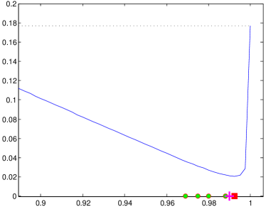
The reference error Eref1subscriptsuperscript𝐸1refE^{1}_{\textup{ref}} in this case is equal to 0.1463, while the minimum error that can be achieved is 0.0816 (-44.22%), corresponding to the couple (λ,μ)=(0.8533,0)superscript𝜆superscript𝜇0.85330(\lambda^{*},\mu^{*})=(0.8533,0) computed by an exhaustive search in the parameter space. Richardson extrapolation method (with s=18𝑠18s=\frac{1}{8}) suggests instead the couple (λR,μR)=(0.29,0.1)superscript𝜆𝑅superscript𝜇𝑅0.290.1(\lambda^{R},\mu^{R})=(0.29,0.1), which is fully inside Φ[W]Φdelimited-[]𝑊\Phi[W] and leads to the error 0.117 (-20.03%). Fig. 4(b) also shows the best coupling parameters (λ,μ)superscript𝜆superscript𝜇(\lambda^{*},\mu^{*}) computed coarsening the grid with s=12,13,14,15𝑠12131415s=\frac{1}{2},\frac{1}{3},\frac{1}{4},\frac{1}{5}. It can be seen that the best coupling parameters do not depend very much on the grid and move monotonically with respect to the scaling from right to left.

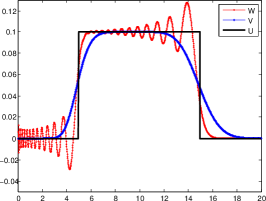
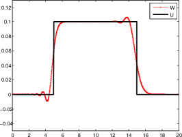
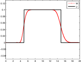
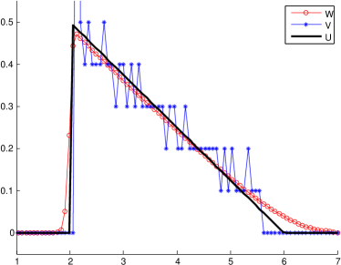
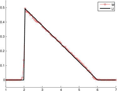
Fig. 5 shows the exact solution UNTsuperscript𝑈subscript𝑁𝑇U^{N_{T}} together with (a) the two uncoupled solutions WNT(1,1)superscript𝑊subscript𝑁𝑇11W^{N_{T}}(1,1) and VNT(1,1)superscript𝑉subscript𝑁𝑇11V^{N_{T}}(1,1), (b) the best coupling WNT(λ,μ)superscript𝑊subscript𝑁𝑇superscript𝜆superscript𝜇W^{N_{T}}(\lambda^{*},\mu^{*}), and (c) the best Richardson coupling WNT(λR,μR)superscript𝑊subscript𝑁𝑇superscript𝜆𝑅superscript𝜇𝑅W^{N_{T}}(\lambda^{R},\mu^{R}) at final time.

Refer to caption Refer to caption Refer to caption
(a) (b) (c)
Figure 5. Test 1: comparison with the exact solution. (a) WNT(1,1)superscript𝑊subscript𝑁𝑇11W^{N_{T}}(1,1) and VNT(1,1)superscript𝑉subscript𝑁𝑇11V^{N_{T}}(1,1). (b) WNT(λ,μ)superscript𝑊subscript𝑁𝑇superscript𝜆superscript𝜇W^{N_{T}}(\lambda^{*},\mu^{*}). (c) WNT(λR,μR)superscript𝑊subscript𝑁𝑇superscript𝜆𝑅superscript𝜇𝑅W^{N_{T}}(\lambda^{R},\mu^{R}).

Note that, although WNT(λR,μR)superscript𝑊subscript𝑁𝑇superscript𝜆𝑅superscript𝜇𝑅W^{N_{T}}(\lambda^{R},\mu^{R}) is worst than WNT(λ,μ)superscript𝑊subscript𝑁𝑇superscript𝜆superscript𝜇W^{N_{T}}(\lambda^{*},\mu^{*}) in terms of L1superscript𝐿1L^{1} error, it does not show spurious oscillations. This is due to the fact that oscillations are sensitive to the grid and then Richardson method easily discards such a solutions.

To better quantify the improvement of the blended scheme with respect to the uncoupled schemes, we found the grid needed by the L1superscript𝐿1L^{1}-best uncoupled scheme (RLW) to achieve the same accuracy of WNT(λR,μR)superscript𝑊subscript𝑁𝑇superscript𝜆𝑅superscript𝜇𝑅W^{N_{T}}(\lambda^{R},\mu^{R}) and WNT(λ,μ)superscript𝑊subscript𝑁𝑇superscript𝜆superscript𝜇W^{N_{T}}(\lambda^{*},\mu^{*}). In the first case we need NC=1704subscript𝑁𝐶1704N_{C}=1704, NT=4260subscript𝑁𝑇4260N_{T}=4260, while in the second case NC=3240subscript𝑁𝐶3240N_{C}=3240, NT=8100subscript𝑁𝑇8100N_{T}=8100, corresponding respectively to a refinement of the grid of a factor 1.421.421.42 and 2.712.712.71.

5.2. Test 2

Test 𝒮1subscript𝒮1\mathcal{S}_{1} 𝒮2subscript𝒮2\mathcal{S}_{2} u¯(x)¯𝑢𝑥\bar{u}(x) ΩΩ\Omega T𝑇T A(x)𝐴𝑥A(x) NCsubscript𝑁𝐶N_{C} NTsubscript𝑁𝑇N_{T} NPsubscript𝑁PN_{\text{P}} β𝛽\beta
2 UPW EE χ[12,32](x)subscript𝜒1232𝑥\chi_{\left[\frac{1}{2},\frac{3}{2}\right]}(x) [0,20]020[0,20] 2.3 x𝑥x 1200 3000 5×NC5subscript𝑁𝐶5\times N_{C} 0.92

In this test we run the multiscale version of the blended scheme coupling UPW and EE in the same setting of Test 1. The UPW error, which will be taken as the reference one, is equal to 0.1771. The minimum error that can be achieved is 0.0204 (-88.48%), corresponding to λ=0.992superscript𝜆0.992\lambda^{*}=0.992 computed by an exhaustive search in the parameter space [0,1]×{1}011[0,1]\times\{1\}. Fig. 6 shows the function λE1[W(λ,1)]𝜆superscript𝐸1delimited-[]𝑊𝜆1\lambda\to E^{1}[W(\lambda,1)] cut by the reference error.

\begin{overpic}[width=195.12767pt]{mMx_batch} \put(85.0,22.0){$\Phi[W]$} \end{overpic} Refer to caption
(a) (b)
Figure 6. Test 2: function λE1[W(λ,1)]𝜆superscript𝐸1delimited-[]𝑊𝜆1\lambda\to E^{1}[W(\lambda,1)] cut by the reference error. (a) λ[0.6,1]𝜆0.61\lambda\in[0.6,1]. (b) λ[0.89,1]𝜆0.891\lambda\in[0.89,1]. The red square indicates the global minimum point λsuperscript𝜆\lambda^{*}, the green circles indicates the global minimum points λsuperscript𝜆\lambda^{*} on coarser grids (s=12,14,16,18𝑠12141618s=\frac{1}{2},\frac{1}{4},\frac{1}{6},\frac{1}{8}), and the magenta cross indicates the Richardson minimum point λRsuperscript𝜆𝑅\lambda^{R}.

Richardson extrapolation method (with s=13𝑠13s=\frac{1}{3}) suggests λR=0.99superscript𝜆𝑅0.99\lambda^{R}=0.99 which leads to the error 0.0208 (-88.26%).

Fig. 7 shows the exact solution UNTsuperscript𝑈subscript𝑁𝑇U^{N_{T}} together with (a) the two uncoupled solutions WNT(1,1)superscript𝑊subscript𝑁𝑇11W^{N_{T}}(1,1) and VNT(1,1)superscript𝑉subscript𝑁𝑇11V^{N_{T}}(1,1), and (b) the best Richardson coupling WNT(λR,1)superscript𝑊subscript𝑁𝑇superscript𝜆𝑅1W^{N_{T}}(\lambda^{R},1) at final time.

Refer to caption Refer to caption
(a) (b)
Figure 7. Test 2: comparison with the exact solution. (a) WNT(1,1)superscript𝑊subscript𝑁𝑇11W^{N_{T}}(1,1) and VNT(1,1)superscript𝑉subscript𝑁𝑇11V^{N_{T}}(1,1). (b) WNT(λR,1)superscript𝑊subscript𝑁𝑇superscript𝜆𝑅1W^{N_{T}}(\lambda^{R},1). Solutions are downsampled for a better viewing.

It can be seen that EE, as opposed to UPW, is rather good in terms of diffusion and in capturing discontinuities, but it has several oscillations. The size of the oscillations depends on NPsubscript𝑁PN_{\text{P}}, while their number depends on NCsubscript𝑁𝐶N_{C}. The vector field A(x)=x𝐴𝑥𝑥A(x)=x tends to separate the particles (but in this case they remains equispaced), therefore the oscillations become larger as the time goes by. Note the the Lagrangian density V(1,1)𝑉11V(1,1) is 0 in those cells not covered by any particle. The blended solution WNT(λR,1)superscript𝑊subscript𝑁𝑇superscript𝜆𝑅1W^{N_{T}}(\lambda^{R},1) combines nicely the advantages of the two schemes, showing little diffusion and tiny oscillations (which have a different nature with respect to those of high-order Eulerian schemes). For the sake of comparison, we report that WENO2 scheme reaches the same accuracy of UPW+EE on a grid refined by a factor 4.2.

We also tested the possibility of localizing the particles around critical zones, namely the discontinuities. At initial time, we locate a few particles across the right discontinuity, and then we activate the blend (with λ=0𝜆0\lambda=0) only in the cells which are between the first and the last particle (more in general, inside the support of the Lagrangian density). This is needed in order to distinguish the two kind of no-particle zones, the one due to the particle rarefaction and the one uncovered by user’s choice. In Fig. 8(a) we show the result of the blended scheme in this case and the region actually covered by particles. The right discontinuity is well caught despite the small number of particles.
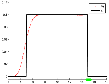
Refer to caption Refer to caption
(a) (b)
Figure 8. Test 2: (a) WNT(0,1)superscript𝑊subscript𝑁𝑇01W^{N_{T}}(0,1) with localized particles. Green circles are the particles. (b) VNT(1,0.3)superscript𝑉subscript𝑁𝑇10.3V^{N_{T}}(1,0.3).

For the sake of completeness, we also report the outcome of the blended scheme whenever the Lagrangian solution is regularized by the Eulerian one. In Fig. 8(b) we show the solution V𝑉V obtained with (λ,μ)=(1,0.3)𝜆𝜇10.3(\lambda,\mu)=(1,0.3). In this case the blend puts together, rather than cancels, the drawbacks of the two uncoupled schemes, leading to a solution which is both diffusive and oscillating.

5.3. Test 3

Test 𝒮1subscript𝒮1\mathcal{S}_{1} 𝒮2subscript𝒮2\mathcal{S}_{2} u¯(x)¯𝑢𝑥\bar{u}(x) ΩΩ\Omega T𝑇T A(x)𝐴𝑥A(x) NCsubscript𝑁𝐶N_{C} NTsubscript𝑁𝑇N_{T} NPsubscript𝑁PN_{\text{P}} β𝛽\beta
3 UPW EE sin(e2x/20)superscript𝑒2𝑥20\sin(e^{2x}/20) [0,π]0𝜋[0,\pi] 111 sin(x)𝑥\sin(x) 600 200 1×NC1subscript𝑁𝐶1\times N_{C} 0.96

In this test we run the multiscale version of the blended scheme coupling UPW and EE in case of a positive space-dependent velocity A(x)=sin(x)𝐴𝑥𝑥A(x)=\sin(x) (for xΩ=[0,π]𝑥Ω0𝜋x\in\Omega=[0,\pi]). The exact solution is

u(x,t)=u¯(γ(x,t))(12tan(x2)(1+e2t)sin(γ(x,t))+etcos(γ(x,t))),γ(x,t)=2arctan(ettan(x2)).formulae-sequence𝑢𝑥𝑡¯𝑢𝛾𝑥𝑡12𝑥21superscript𝑒2𝑡𝛾𝑥𝑡superscript𝑒𝑡𝛾𝑥𝑡𝛾𝑥𝑡2superscript𝑒𝑡𝑥2u(x,t)=\bar{u}(\gamma(x,t))\left(\frac{1}{2}\tan\left(\frac{x}{2}\right)\left(1+e^{-2t}\right)\sin(\gamma(x,t))+e^{-t}\cos(\gamma(x,t))\right),\quad\gamma(x,t)=2\arctan\left(e^{-t}\tan\left(\frac{x}{2}\right)\right).

The reference error (UPW) in this case is equal to 0.2591. Fig. 9 shows the exact solution UNTsuperscript𝑈subscript𝑁𝑇U^{N_{T}} together with the two uncoupled solutions WNT(1,1)superscript𝑊subscript𝑁𝑇11W^{N_{T}}(1,1) and VNT(1,1)superscript𝑉subscript𝑁𝑇11V^{N_{T}}(1,1) at final time. In this case the particles move rightward accumulating on the right side of the domain.
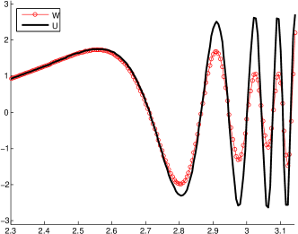
Refer to caption Refer to caption
(a) (b)
Figure 9. Test 3: uncoupled schemes in [2.3,π]2.3𝜋[2.3,\pi]. (a) WNT(1,1)superscript𝑊subscript𝑁𝑇11W^{N_{T}}(1,1). (b) VNT(1,1)superscript𝑉subscript𝑁𝑇11V^{N_{T}}(1,1).

The minimum error that can be achieved is 0.0731 (-71.79%), corresponding to λ=0.93superscript𝜆0.93\lambda^{*}=0.93. Richardson extrapolation method (with s=12𝑠12s=\frac{1}{2}) suggests instead λR=0.916superscript𝜆𝑅0.916\lambda^{R}=0.916, which leads to the error 0.0742 (-71.36%).

Fig. 10 shows four blended solutions obtained with different choices of λ𝜆\lambda. For low values of the coupling parameter (λ=0.8𝜆0.8\lambda=0.8) the solution is accurate where the number of particles is large (right side) but not where there are no or a few particles (left side). The situation is reversed for large values of the coupling parameter (λ=0.99𝜆0.99\lambda=0.99). The Richardson solution λ=λR=0.916𝜆superscript𝜆𝑅0.916\lambda=\lambda^{R}=0.916 reaches a good compromise between the two cases. On the other hand, an even better result can be obtained by means of a variable-in-space λ=λ(Λ)𝜆𝜆Λ\lambda=\lambda(\Lambda) (see Section 2.2 for the definition of ΛΛ\Lambda). Last plot in Fig. 10 shows the result of an hand-tuned decreasing function λ(Λ)𝜆Λ\lambda(\Lambda) which leads to a good accuracy in both sides of the domain.
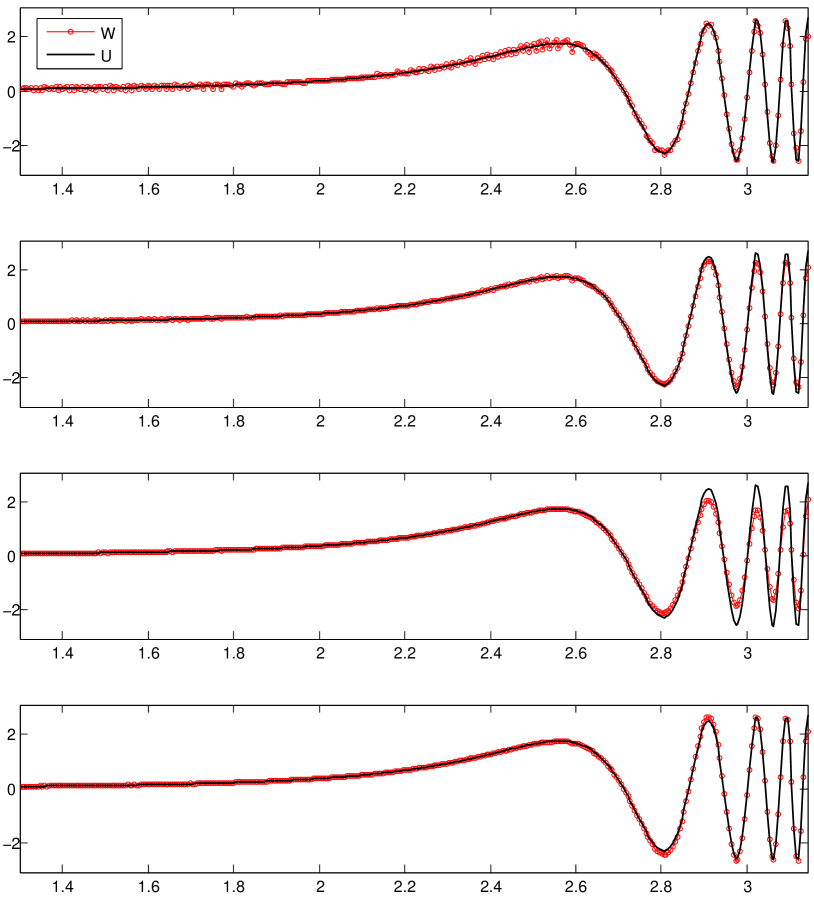
Refer to caption
Figure 10. Test 3: WNT(λ,1)superscript𝑊subscript𝑁𝑇𝜆1W^{N_{T}}(\lambda,1) in [1.3,π]1.3𝜋[1.3,\pi] for different choices of λ𝜆\lambda. from top to bottom: λ=0.8𝜆0.8\lambda=0.8 (E1=0.1085superscript𝐸10.1085E^{1}=0.1085), λ=λR=0.952𝜆superscript𝜆𝑅0.952\lambda=\lambda^{R}=0.952 (E1=0.0764superscript𝐸10.0764E^{1}=0.0764), λ=0.99𝜆0.99\lambda=0.99 (E1=0.1517superscript𝐸10.1517E^{1}=0.1517), λ=λ(Λ)𝜆𝜆Λ\lambda=\lambda(\Lambda) (E1=0.0396superscript𝐸10.0396E^{1}=0.0396).

5.4. Test 4

Test 𝒮1subscript𝒮1\mathcal{S}_{1} 𝒮2subscript𝒮2\mathcal{S}_{2} u¯(x)¯𝑢𝑥\bar{u}(x) ΩΩ\Omega T𝑇T f(u)𝑓𝑢f(u) NCsubscript𝑁𝐶N_{C} NTsubscript𝑁𝑇N_{T} NPsubscript𝑁PN_{\text{P}} β𝛽\beta
4 GODUNOV EE 12χ[0,2](x)12subscript𝜒02𝑥\frac{1}{2}\chi_{\left[0,2\right]}(x) [0.2,7]0.27[-0.2,7] 444 u(1u)𝑢1𝑢u(1-u) 100 200 5×NC5subscript𝑁𝐶5\times N_{C} 0.28

In this test we solve equation (3) with f(u)=u(1u)𝑓𝑢𝑢1𝑢f(u)=u(1-u) (LWR model for traffic flow). The exact solution is u(x,T)=18x+34𝑢𝑥𝑇18𝑥34u(x,T)=-\frac{1}{8}x+\frac{3}{4} in [2,6]26[2,6] and u(x,T)=0𝑢𝑥𝑇0u(x,T)=0 elsewhere. A rarefaction and a shock are present. The reference error (GODUNOV) in this case is equal to 0.0839. Richardson extrapolation method (with s=12𝑠12s=\frac{1}{2}) suggests λR=0.956superscript𝜆𝑅0.956\lambda^{R}=0.956 which leads to the error 0.0317 (-62.22%). Here we used W𝑊W to evaluate the particles’ velocity, see (13). Fig. 11 shows the exact solution UNTsuperscript𝑈subscript𝑁𝑇U^{N_{T}} together with (a) the two uncoupled solutions WNT(1,1)superscript𝑊subscript𝑁𝑇11W^{N_{T}}(1,1) and VNT(1,1)superscript𝑉subscript𝑁𝑇11V^{N_{T}}(1,1), and (b) the best Richardson coupling WNT(λR,1)superscript𝑊subscript𝑁𝑇superscript𝜆𝑅1W^{N_{T}}(\lambda^{R},1) at final time.

Refer to caption Refer to caption
(a) (b)
Figure 11. Test 4: comparison with the exact solution. (a) WNT(1,1)superscript𝑊subscript𝑁𝑇11W^{N_{T}}(1,1) and VNT(1,1)superscript𝑉subscript𝑁𝑇11V^{N_{T}}(1,1). (b) WNT(λR,1)superscript𝑊subscript𝑁𝑇superscript𝜆𝑅1W^{N_{T}}(\lambda^{R},1).

Conclusions and perspectives

We proposed a new method for coupling two (or more) explicit schemes approximating advection equations and scalar conservation laws. We provided some convergence analysis and we showed that effective couplings can be obtained in practice using a standard Richardson extrapolation. Moreover, several numerical tests confirmed that, whenever the constitutive schemes are respectively an Eulerian (macroscopic) and a Lagrangian (particle based) scheme, the blended scheme gives rather accurate results despite its Eulerian part gives only a low order approximation. This is a remarkable advantage, since it is well known that implementing high-order solvers is much easier for ODEs than for PDEs.

It is interesting to note that the blended scheme can be put in relation with very different schemes proposed in the literature, see Section 1.

  • If the coupling parameters are allowed to depend on space and/or on the solution itself, we can blend Eulerian schemes of different orders to recover the constitutive ideas of the filtered schemes.

  • Coupling an Eulerian scheme with a pure Lagrangian scheme and localizing particles, we recover a scheme that resembles that of the particle level-set method.

  • Annealing the Eulerian scheme but keeping alive the coupling with (λ,μ)=(0,1)𝜆𝜇01(\lambda,\mu)=(0,1), we recover a scheme that resembles that of the particle-in-cell method.

  • The multiscale blended scheme (with μ=1𝜇1\mu=1) seems to follow the opposite philosophy with respect to the smoothed-particle hydrodynamics method. While the latter regularizes the Lagrangian solution by a suitable choice of smoothing kernels, the former “Dirac-izes” the Eulerian solution. Moreover, the computation of the optimal blending parameter resembles the computation of the optimal supports for the smoothing kernels.

Finally, let us mention that one of the most promising and yet unexplored feature of the blended scheme is the parallelization on distributed-memory architectures. Particle evolution is indeed embarrassingly parallel (within a time step), since there is no need to locate the neighbouring particles of a given one (which can be a severe bottleneck if particles live in different memory units).

Acknowledgements

The authors thank R. Natalini who, commenting the paper [4], one day asked: “Does the microscopic coupling decrease the numerical diffusion?”. E. Cristiani also wants to thank S. Succi for the motivating discussions and A. Di Mascio for the useful suggestions.

References

  • [1] C. K. Birdsall and A. B. Langdon, Plasma Physics Via Computer Simulation, CRC Press, Boca Raton, 2004.
  • [2] E. Carlini, R. Ferretti and G. Russo, A weighted essentially nonoscillatory, large time-step scheme for Hamilton-Jacobi equations, SIAM J. Sci. Comput., 27 (2005), 1071–1091.
  • [3] E. Cristiani, Blending Brownian motion and heat equation, J. Coupled Syst. Multiscale Dyn., 3 (2015), 351–356.
  • [4] E. Cristiani, B. Piccoli and A. Tosin, Multiscale modeling of granular flows with application to crowd dynamics, Multiscale Model. Simul., 9 (2011), 155–182.
  • [5] W. E, Principles of multiscale modeling, Cambridge University Press, 2011.
  • [6] D. Enright, R. Fedkiw, J. Ferziger and I. Mitchell, A hybrid particle level set method for improved interface capturing, J. Comp. Phys., 183 (2002), 83–116.
  • [7] M. Falcone and R. Ferretti, Semi-Lagrangian approximation schemes for linear and Hamilton-Jacobi equations, SIAM, 2014.
  • [8] B. D. Froese and A. M. Oberman, Fast finite difference solvers for singular solutions of the elliptic Monge-Ampère equation, J. Comput. Phys., 230 (2011), 818–834.
  • [9] B. D. Froese and A. M. Oberman, Convergent filtered schemes for the Monge-Ampère partial differential equation, SIAM J. Numer. Anal., 51 (2013), 423–444.
  • [10] R.A. Gingold and J.J. Monaghan, Smoothed particle hydrodynamics: theory and application to non-spherical stars, Mon. Not. R. Astron. Soc., 181 (1977), 375–389.
  • [11] A. Harten, B. Engquist, S. Osher and S. R. Chakravarthy, Uniformly high order accurate essentially non-oscillatory schemes, III, J. Comput. Phys., 71 (1987), 231–303.
  • [12] S.-I. Inutsuka, Reformulation of smoothed particle hydrodynamics with Riemann solver, J. Comput. Phys., 179 (2002), 238–267.
  • [13] R. J. LeVeque, Numerical methods for conservation laws, Birkhäuser, 1992.
  • [14] X.-D. Liu, S. Osher and T. Chan, Weighted essentially non-oscillatory schemes, J. Comput. Phys., 115 (1994), 200–212.
  • [15] L.B. Lucy, A numerical approach to the testing of the fission hypothesis, Astron. J., 82 (1977), 1013–1024.
  • [16] S. Marrone, A. Di Mascio and D. Le Touzé, Coupling of Smoothed Particle Hydrodynamics with Finite Volume method for free-surface flows, J. Comput. Phys., 310 (2016), 161–180.
  • [17] A. M. Oberman and T. Salvador, Filtered schemes for Hamilton-Jacobi equations: A simple construction of convergent accurate difference schemes, J. Comput. Phys., 284 (2015), 367–388.
  • [18] S. Osher and J. A. Sethian, Fronts propagating with curvature-dependent speed: Algorithms based on Hamilton-Jacobi formulations, J. Comput. Phys., 79 (1988), 12–49.
  • [19] Kunal Puri and Prabhu Ramachandran, Approximate Riemann solvers for the Godunov SPH (GSPH), J. Comput. Phys., 270 (2014), 432–458.
  • [20] C.-W. Shu, Essentially non-oscillatory and weighted essentially non-oscillatory schemes for hyperbolic conservation laws, NASA/CR-97-206253, ICASE Report No. 97-65, 1997.