String and Membrane Gaussian Processes

\nameYves-Laurent Kom Samo \emailylks@robots.ox.ac.uk \AND\nameStephen J. Roberts \emailsjrob@robots.ox.ac.uk
\addrDepartment of Engineering Science and Oxford-Man Institute
University of Oxford
Eagle House, Walton Well Road,
OX2 6ED, Oxford, United Kingdom
Abstract

In this paper we introduce a novel framework for making exact nonparametric Bayesian inference on latent functions that is particularly suitable for Big Data tasks. Firstly, we introduce a class of stochastic processes we refer to as string Gaussian processes (string GPs which are not to be mistaken for Gaussian processes operating on text). We construct string GPs so that their finite-dimensional marginals exhibit suitable local conditional independence structures, which allow for scalable, distributed, and flexible nonparametric Bayesian inference, without resorting to approximations, and while ensuring some mild global regularity constraints. Furthermore, string GP priors naturally cope with heterogeneous input data, and the gradient of the learned latent function is readily available for explanatory analysis. Secondly, we provide some theoretical results relating our approach to the standard GP paradigm. In particular, we prove that some string GPs are Gaussian processes, which provides a complementary global perspective on our framework. Finally, we derive a scalable and distributed MCMC scheme for supervised learning tasks under string GP priors. The proposed MCMC scheme has computational time complexity 𝒪(N)𝒪𝑁\mathcal{O}(N) and memory requirement 𝒪(dN)𝒪𝑑𝑁\mathcal{O}(dN), where N𝑁N is the data size and d𝑑d the dimension of the input space. We illustrate the efficacy of the proposed approach on several synthetic and real-world data sets, including a data set with 666 millions input points and 888 attributes.

Keywords: String Gaussian processes, scalable Bayesian nonparametrics, Gaussian processes, nonstationary kernels, reversible-jump MCMC, point process priors

1 Introduction

Many problems in statistics and machine learning involve inferring a latent function from training data (for instance regression, classification, inverse reinforcement learning, inference on point processes to name but a few). Real-valued stochastic processes, among which Gaussian processes (GPs), are often used as functional priors for such problems, thereby allowing for a full Bayesian nonparametric treatment. In the machine learning community, interest in GPs grew out of the observation that some Bayesian neural networks converge to GPs as the number of hidden units approaches infinity (Neal (1996)). Since then, other similarities have been established between GPs and popular models such as Bayesian linear regression, Bayesian basis function regression, spline models and support vector machines (Rasmussen and Williams (2006)). However, they often perform poorly on Big Data tasks primarily for two reasons. Firstly, large data sets are likely to exhibit multiple types of local patterns that should appropriately be accounted for by flexible and possibly nonstationary covariance functions, the development of which is still an active subject of research. Secondly, inference under GP priors often consists of looking at the values of the GP at all input points as a jointly Gaussian vector with fully dependent coordinates, which induces a memory requirement and time complexity respectively squared and cubic in the training data size, and thus is intractable for large data sets. We refer to this approach as the standard GP paradigm. The framework we introduce in this paper addresses both of the above limitations.

Our work is rooted in the observation that, from a Bayesian nonparametric perspective, it is inefficient to define a stochastic process through fully-dependent marginals, as it is the case for Gaussian processes. Indeed, if a stochastic process (f(x))xdsubscript𝑓𝑥𝑥superscript𝑑(f(x))_{x\in\mathbb{R}^{d}} has fully dependent marginals and exhibits no additional conditional independence structure then, when f𝑓f is used as functional prior and some observations related to (f(x1),,f(xn))𝑓subscript𝑥1𝑓subscript𝑥𝑛\left(f(x_{1}),\dots,f(x_{n})\right) are gathered, namely (y1,,yn)subscript𝑦1subscript𝑦𝑛\left(y_{1},\dots,y_{n}\right), the additional memory required to take into account an additional piece of information (yn+1,xn+1)subscript𝑦𝑛1subscript𝑥𝑛1(y_{n+1},x_{n+1}) grows in 𝒪(n)𝒪𝑛\mathcal{O}(n), as one has to keep track of the extent to which yn+1subscript𝑦𝑛1y_{n+1} informs us about f(xi)𝑓subscript𝑥𝑖f(x_{i}) for every in𝑖𝑛i\leq n, typically through a covariance matrix whose size will increase by 2n+12𝑛12n+1 terms. Clearly, this is inefficient, as yn+1subscript𝑦𝑛1y_{n+1} is unlikely to be informative about f(xi)𝑓subscript𝑥𝑖f(x_{i}), unless xisubscript𝑥𝑖x_{i} is sufficiently close to xn+1subscript𝑥𝑛1x_{n+1}. More generally, the larger n𝑛n, the less information a single additional pair (yn+1,xn+1)subscript𝑦𝑛1subscript𝑥𝑛1(y_{n+1},x_{n+1}) will add to existing data, and yet the increase in memory requirement will be much higher than that required while processing earlier and more informative data. This inefficiency in resource requirements extends to computational time, as the increase in computational time resulting from adding (yn+1,xn+1)subscript𝑦𝑛1subscript𝑥𝑛1(y_{n+1},x_{n+1}) typically grows in 𝒪(n2)𝒪superscript𝑛2\mathcal{O}(n^{2}), which is the difference between the numbers of operations required to invert a n×n𝑛𝑛n\times n matrix and to invert a (n+1)×(n+1)𝑛1𝑛1(n+1)\times(n+1) matrix. A solution for addressing this inefficiency is to appropriately limit the extent to which values f(x1),,f(xn)𝑓subscript𝑥1𝑓subscript𝑥𝑛f(x_{1}),\dots,f(x_{n}) are related to each other. Existing approaches such as sparse Gaussian processes (see Quinonero-Candela and Rasmussen (2005) for a review), resort to an ex-post approximation of fully-dependent Gaussian marginals with multivariate Gaussians exhibiting conditional independence structures. Unfortunately, these approximations trade-off accuracy for scalability through a control variable, namely the number of inducing points, whose choice is often left to the user. The approach we adopt in this paper consists of going back to stochastic analysis basics, and constructing stochastic processes whose finite-dimensional marginals exhibit suitable conditional independence structures so that we need not resorting to ex-post approximations. Incidentally, unlike sparse GP techniques, the conditional independence structures we introduce also allow for flexible and principled learning of local patterns, and this increased flexibility does not come at the expense of scalability.

The contributions of this paper are as follows. We introduce a novel class of stochastic processes, string Gaussian processes (string GPs), that may be used as priors over latent functions within a Bayesian nonparametric framework, especially for large scale problems and in the presence of possibly multiple types of local patterns. We propose a framework for analysing the flexibility of random functions and surfaces, and prove that our approach yields more flexible stochastic processes than isotropic Gaussian processes. We demonstrate that exact inference under a string GP prior scales considerably better than in the standard GP paradigm, and is amenable to distributed computing. We illustrate that popular stationary kernels can be well approximated within our framework, making string GPs a scalable alternative to commonly used GP models. We derive the joint law of a string GP and its gradient, thereby allowing for explanatory analysis on the learned latent function. We propose a reversible-jump Markov Chain Monte Carlo sampler for automatic learning of model complexity and local patterns from data.

The rest of the paper is structured as follows. In Section 2 we review recent advances on Gaussian processes in relation to inference on large data sets. In Section 3 we formally construct string GPs and derive some important results. In Section 4 we provide detailed illustrative and theoretical comparisons between string GPs and the standard GP paradigm. In Section 5 we propose methods for inferring latent functions under string GP priors with time complexity and memory requirement that are linear in the size of the data set. The efficacy of our approach compared to competing alternatives is illustrated in Section 6. Finally, we finish with a discussion in Section 7.

2 Related Work

The two primary drawbacks of the standard GP paradigm on large scale problems are the lack of scalability resulting from postulating a full multivariate Gaussian prior on function values at all training inputs, and the difficulty postulating a priori a class of covariance functions capable of capturing intricate and often local patterns likely to occur in large data sets. A tremendous amount of work has been published that attempt to address either of the aforementioned limitations. However, scalability is often achieved either through approximations or for specific applications, and nonstationarity is usually introduced at the expense of scalability, again for specific applications.

2.1 Scalability Through Structured Approximations

As far as scalability is concerned, sparse GP methods have been developed that approximate the multivariate Gaussian probability density function (pdf) over training data with the marginal over a smaller set of inducing points multiplied by an approximate conditional pdf (Smola and Bartlett (2001); Lawrence et al. (2003); Seeger (2003b, a); Snelson and Ghahramani (2006)). This approximation yields a time complexity linear—rather than cubic—in the data size and squared in the number of inducing points. We refer to Quinonero-Candela and Rasmussen (2005) for a review of sparse GP approximations. More recently, Hensman et al. (2013, 2015) combined sparse GP methods with Stochastic Variational Inference (Hoffman et al. (2013)) for GP regression and GP classification. However, none of these sparse GP methods addresses the selection of the number of inducing points (and the size of the minibatch in the case of Hensman et al. (2013, 2015)), although this may greatly affect scalability. More importantly, although these methods do not impose strong restrictions on the covariance function of the GP model to approximate, they do not address the need for flexible covariance functions inherent to large scale problems, which are more likely to exhibit intricate and local patterns, and applications considered by the authors typically use the vanilla squared exponential kernel.

Lazaro-Gredilla et al. (2010) proposed approximating stationary kernels with truncated Fourier series in Gaussian process regression. An interpretation of the resulting sparse spectrum Gaussian process model as Bayesian basis function regression with a finite number K𝐾K of trigonometric basis functions allows making inference in time complexity and memory requirement that are both linear in the size of the training sample. However, this model has two major drawbacks. Firstly, it is prone to over-fitting. In effect, the learning machine will aim at inferring the K𝐾K major spectral frequencies evidenced in the training data. This will only lead to appropriate prediction out-of-sample when the underlying latent phenomenon can be appropriately characterised by a finite discrete spectral decomposition that is expected to be the same everywhere on the domain. Secondly, this model implicitly postulates that the covariance between the values of the GP at two points does not vanish as the distance between the points becomes arbitrarily large. This imposes a priori the view that the underlying function is highly structured, which might be unrealistic in many real-life non-periodic applications. This approach is generalised by the so-called random Fourier features methods (Rahimi and Recht (2007); Le et al. (2013); Yang et al. (2015)). Unfortunately all existing random Fourier features methods give rise to stationary covariance functions, which might not be appropriate for data sets exhibiting local patterns.

The bottleneck of inference in the standard GP paradigm remains inverting and computing the determinant of a covariance matrix, normally achieved through the Cholesky decomposition or Singular Value Decomposition. Methods have been developed that speed-up these decompositions through low rank approximations (Williams and Seeger (2001)) or by exploiting specific structures in the covariance function and in the input data (Saatchi (2011); Wilson et al. (2014)), which typically give rise to Kronecker or Toeplitz covariance matrices. While the Kronecker method used by Saatchi (2011) and Wilson et al. (2014) is restricted to inputs that form a Cartesian grid and to separable kernels,111That is multivariate kernel that can be written as product of univariate kernels. low rank approximations such as the Nystro¨¨o\ddot{\text{o}}m method used by Williams and Seeger (2001) modify the covariance function and hence the functional prior in a non-trivial way. Methods have also been proposed to interpolate the covariance matrix on a uniform or Cartesian grid in order to benefit from some of the computational gains of Toeplitz and Kronecker techniques even when the input space is not structured (Wilson and Nickisch (2015)). However, none of these solutions is general as they require that either the covariance function be separable (Kronecker techniques), or the covariance function be stationary and the input space be one-dimensional (Toeplitz techniques).

2.2 Scalability Through Data Distribution

A family of methods have been proposed to scale-up inference in GP models that are based on the observation that it is more computationally efficient to compute the pdf of K𝐾K independent small Gaussian vectors with size n𝑛n than to compute the pdf of a single bigger Gaussian vector of size nK𝑛𝐾nK. For instance, Kim et al. (2005) and Gramacy and Lee (2008) partitioned the input space, and put independent stationary GP priors on the restrictions of the latent function to the subdomains forming the partition, which can be regarded as independent local GP experts. Kim et al. (2005) partitioned the domain using Voronoi tessellations, while Gramacy and Lee (2008) used tree based partitioning. These two approaches are provably equivalent to postulating a (nonstationary) GP prior on the whole domain that is discontinuous along the boundaries of the partition, which might not be desirable if the latent function we would like to infer is continuous, and might affect predictive accuracy. The more local experts there are, the more scalable the model will be, but the more discontinuities the latent function will have, and subsequently the less accurate the approach will be.

Mixtures of Gaussian process experts models (MoE) (Tresp (2001); Rasmussen and Ghahramani (2001); Meeds and Osindero (2006); Ross and Dy (2013)) provide another implementation of this idea. MoE models assume that there are multiple latent functions to be inferred from the data, on which it is placed independent GP priors, and each training input is associated to one latent function. The number of latent functions and the repartition of data between latent functions can then be performed in a full Bayesian nonparametric fashion (Rasmussen and Ghahramani (2001); Ross and Dy (2013)). When there is a single continuous latent function to be inferred, as it is the case for most regression models, the foregoing Bayesian nonparametric approach will learn a single latent function, thereby leading to a time complexity and a memory requirement that are the same as in the standard GP paradigm, which defies the scalability argument.

The last implementation of the idea in this section consists of distributing the training data over multiple independent but identical GP models. In regression problems, examples include the Bayesian Committee Machines (BCM) of Tresp (2000), the generalized product of experts (gPoE) model of Cao and Fleet (2014), and the robust Bayesian Committee Machines (rBCM) of Deisenroth and Ng (2015). These models propose splitting the training data in small subsets, each subset being assigned to a different GP regression model—referred to as an expert—that has the same hyper-parameters as the other experts, although experts are assumed to be mutually independent. Training is performed by maximum marginal likelihood, with time complexity (resp. memory requirement) linear in the number of experts and cubic (resp. squared) in the size of the largest data set processed by an expert. Predictions are then obtained by aggregating the predictions of all GP experts in a manner that is specific to the method used (that is the BCM, the gPoE or the rBCM). However, these methods present major drawbacks in the training and testing procedures. In effect, the assumption that experts have identical hyper-parameters is inappropriate for data sets exhibiting local patterns. Even if one would allow GP experts to be driven by different hyper-parameters as in Nguyen and Bonilla (2014) for instance, learned hyper-parameters would lead to overly simplistic GP experts and poor aggregated predictions when the number of training inputs assigned to each expert is small—this is a direct consequence of the (desirable) fact that maximum marginal likelihood GP regression abides by Occam’s razor. Another critical pitfall of BCM, gPoE and rBCM is that their methods for aggregating expert predictions are Kolmogorov inconsistent. For instance, denoting p^^𝑝\hat{p} the predictive distribution in the BCM, it can be easily seen from Equations (2.4) and (2.5) in Tresp (2000) that the predictive distribution p^(f(x1)|𝒟)^𝑝conditional𝑓superscriptsubscript𝑥1𝒟\hat{p}(f(x_{1}^{*})|\mathcal{D}) (resp. p^(f(x2)|𝒟)^𝑝conditional𝑓superscriptsubscript𝑥2𝒟\hat{p}(f(x_{2}^{*})|\mathcal{D}))222Here f𝑓f is the latent function to be inferred, x1,x2superscriptsubscript𝑥1superscriptsubscript𝑥2x_{1}^{*},x_{2}^{*} are test points and 𝒟𝒟\mathcal{D} denotes training data. provided by the aggregation procedure of the BCM is not the marginal over f(x2)𝑓superscriptsubscript𝑥2f(x_{2}^{*}) (resp. over f(x1)𝑓superscriptsubscript𝑥1f(x_{1}^{*})) of the multivariate predictive distribution p^(f(x1),f(x2)|𝒟)^𝑝𝑓superscriptsubscript𝑥1conditional𝑓superscriptsubscript𝑥2𝒟\hat{p}(f(x_{1}^{*}),f(x_{2}^{*})|\mathcal{D}) obtained from experts multivariate predictions pk(f(x1),f(x2)|𝒟)subscript𝑝𝑘𝑓superscriptsubscript𝑥1conditional𝑓superscriptsubscript𝑥2𝒟p_{k}(f(x_{1}^{*}),f(x_{2}^{*})|\mathcal{D}) using the same aggregation procedure: p^(f(x1)|𝒟)p^(f(x1),f(x2)|𝒟)𝑑f(x2)^𝑝conditional𝑓superscriptsubscript𝑥1𝒟^𝑝𝑓superscriptsubscript𝑥1conditional𝑓superscriptsubscript𝑥2𝒟differential-d𝑓superscriptsubscript𝑥2\hat{p}(f(x_{1}^{*})|\mathcal{D})\neq\int\hat{p}(f(x_{1}^{*}),f(x_{2}^{*})|\mathcal{D})df(x_{2}^{*}). Without Kolmogorov consistency, it is impossible to make principled Bayesian inference of latent function values. A principled Bayesian nonparametric model should not provide predictions about f(x1)𝑓superscriptsubscript𝑥1f(x_{1}^{*}) that differ depending on whether or not one is also interested in predicting other values f(xi)𝑓superscriptsubscript𝑥𝑖f(x_{i}^{*}) simultaneously. This pitfall might be the reason why Cao and Fleet (2014) and Deisenroth and Ng (2015) restricted their expositions to predictive distributions about a single function value at a time p^(f(x)|𝒟)^𝑝conditional𝑓superscript𝑥𝒟\hat{p}(f(x^{*})|\mathcal{D}), although their procedures (Equation 4 in Cao and Fleet (2014) and Equation 20 in Deisenroth and Ng (2015)) are easily extended to posterior distributions over multiple function values. These extensions would also be Kolmogorov inconsistent, and restricting the predictions to be of exactly one function value is unsatisfactory as it does not allow determining the posterior covariance between function values at two test inputs.

2.3 Expressive Stationary Kernels

In regards to flexibly handling complex patterns likely to occur in large data sets, Wilson and Adams (2013) introduced a class of expressive stationary kernels obtained by summing up convolutions of Gaussian basis functions with Dirac delta functions in the spectral domain. The sparse spectrum kernel can be thought of as the special case where the convolving Gaussian is degenerate. Although such kernels perform particularly well in the presence of globally repeated patterns in the data, their stationarity limits their utility on data sets with local patterns. Moreover the proposed covariance functions generate infinitely differentiable random functions, which might be too restrictive in some applications.

2.4 Application-Specific Nonstationary Kernels

As for nonstationary kernels, Paciorek and Schervish (2004) proposed a method for constructing nonstationary covariance functions from any stationary one that involves introducing n𝑛n input dependent d×d𝑑𝑑d\times d covariance matrices that will be inferred from the data. Plagemann et al. (2008) proposed a faster approximation to the model of Paciorek and Schervish (2004). However, both approaches scale poorly with the input dimension and the data size as they have time complexity 𝒪(max(nd3,n3))𝒪𝑛superscript𝑑3superscript𝑛3\mathcal{O}\left(\max(nd^{3},n^{3})\right). MacKay (1998), Schmidt and O’Hagan (2003), and Calandra et al. (2014) proposed kernels that can be regarded as stationary after a non-linear transformation d𝑑d on the input space: k(x,x)=h(d(x)d(x)),𝑘𝑥superscript𝑥norm𝑑𝑥𝑑superscript𝑥k(x,x^{\prime})=h\left(\|d(x)-d(x^{\prime})\|\right), where hh is positive semi-definite. Although for a given deterministic function d𝑑d the kernel k𝑘k is nonstationary, Schmidt and O’Hagan (2003) put a GP prior on d𝑑d with mean function m(x)=x𝑚𝑥𝑥m(x)=x and covariance function invariant under translation, which unfortunately leads to a kernel that is (unconditionally) stationary, albeit more flexible than h(xx).norm𝑥superscript𝑥h\left(\|x-x^{\prime}\|\right). To model nonstationarity, Adams and Stegle (2008) introduced a functional prior of the form y(x)=f(x)expg(x)𝑦𝑥𝑓𝑥𝑔𝑥y(x)=f(x)\exp{g(x)} where f𝑓f is a stationary GP and g𝑔g is some scaling function on the domain. For a given non-constant function g𝑔g such a prior indeed yields a nonstationary Gaussian process. However, when a stationary GP prior is placed on the function g𝑔g as Adams and Stegle (2008) did, the resulting functional prior y(x)=f(x)expg(x)𝑦𝑥𝑓𝑥𝑔𝑥y(x)=f(x)\exp{g(x)} becomes stationary. The piecewise GP (Kim et al. (2005)) and treed GP (Gramacy and Lee (2008)) models previously discussed also introduce nonstationarity. The authors’ premise is that heterogeneous patterns might be locally homogeneous. However, as previously discussed such models are inappropriate for modelling continuous latent functions.

2.5 Our Approach

The approach we propose in this paper for inferring latent functions in large scale problems, possibly exhibiting locally homogeneous patterns, consists of constructing a novel class of smooth, nonstationary and flexible stochastic processes we refer to as string Gaussian processes (string GPs), whose finite dimensional marginals are structured enough so that full Bayesian nonparametric inference scales linearly with the sample size, without resorting to approximations. Our approach is analogous to MoE models in that, when the input space is one-dimensional, a string GP can be regarded as a collaboration of local GP experts on non-overlapping supports, that implicitly exchange messages with one another, and that are independent conditional on the aforementioned messages. Each local GP expert only shares just enough information with adjacent local GP experts for the whole stochastic process to be sufficiently smooth (for instance continuously differentiable), which is an important improvement over MoE models as the latter generate discontinuous latent functions. These messages will take the form of boundary conditions, conditional on which each local GP expert will be independent from any other local GP expert. Crucially, unlike the BCM, the gPoE and the rBCM, we do not assume that local GP experts share the same prior structure (that is mean function, covariance function, or hyper-parameters). This allows each local GP expert to flexibly learn local patterns from the data if there are any, while preserving global smoothness, which will result in improved accuracy. Similarly to MoEs, the computational gain in our approach stems from the fact that the conditional independence of the local GP experts conditional on shared boundary conditions will enable us to write the joint distribution over function and derivative values at a large number of inputs as the product of pdfs of much smaller Gaussian vectors. The resulting effect on time complexity is a decrease from 𝒪(N3)𝒪superscript𝑁3\mathcal{O}(N^{3}) to 𝒪(max𝑘nk3)𝒪𝑘superscriptsubscript𝑛𝑘3\mathcal{O}(\underset{k}{\max}~{}n_{k}^{3}), where N=knk,nkNformulae-sequence𝑁subscript𝑘subscript𝑛𝑘much-less-thansubscript𝑛𝑘𝑁N=\sum_{k}n_{k},~{}n_{k}\ll N. In fact, in Section 5 we will propose Reversible-Jump Monte Carlo Markov Chain (RJ-MCMC) inference methods that achieve memory requirement and time complexity 𝒪(N)𝒪𝑁\mathcal{O}(N), without any loss of flexibility. All these results are preserved by our extension of string GPs to multivariate input spaces, which we will occasionally refer to as membrane Gaussian processes (or membrane GPs). Unlike the BCM, the gPoE and the rBCM, the approach we propose in this paper, which we will refer to as the string GP paradigm, is Kolmogorov consistent, and enables principled inference of the posterior distribution over the values of the latent function at multiple test inputs.

3 Construction of String and Membrane Gaussian Processes

In this section we formally construct string Gaussian processes, and we provide some important theoretical results including smoothness, and the joint law of string GPs and their gradients. We construct string GPs indexed on \mathbb{R}, before generalising to string GPs indexed on dsuperscript𝑑\mathbb{R}^{d}, which we will occasionally refer to as membrane GPs to stress that the input space is multivariate. We start by considering the joint law of a differentiable GP on an interval and its derivative, and introducing some related notions that we will use in the construction of string GPs.

Proposition 1

(Derivative Gaussian processes)
Let I𝐼I be an interval, k:I×I:𝑘𝐼𝐼k:I\times I\rightarrow\mathbb{R} a 𝒞2superscript𝒞2\mathcal{C}^{2} symmetric positive semi-definite function,333𝒞1superscript𝒞1\mathcal{C}^{1} (resp. 𝒞2superscript𝒞2\mathcal{C}^{2}) functions denote functions that are once (resp. twice) continuously differentiable on their domains. m:I:𝑚𝐼m:I\rightarrow\mathbb{R} a 𝒞1superscript𝒞1\mathcal{C}^{1} function.

(A) There exists a 2superscript2\mathbb{R}^{2}-valued stochastic process (Dt)tI,Dt=(zt,zt)subscriptsubscript𝐷𝑡𝑡𝐼subscript𝐷𝑡subscript𝑧𝑡superscriptsubscript𝑧𝑡\left(D_{t}\right)_{t\in I},~{}D_{t}=(z_{t},z_{t}^{\prime}), such that for all t1,,tnIsubscript𝑡1subscript𝑡𝑛𝐼t_{1},\dots,t_{n}\in I, (zt1,,ztn,zt1,,ztn)subscript𝑧subscript𝑡1subscript𝑧subscript𝑡𝑛superscriptsubscript𝑧subscript𝑡1superscriptsubscript𝑧subscript𝑡𝑛(z_{t_{1}},\dots,z_{t_{n}},z_{t_{1}}^{\prime},\dots,z_{t_{n}}^{\prime}) is a Gaussian vector with mean (m(t1),,m(tn),dmdt(t1),,dmdt(tn))𝑚subscript𝑡1𝑚subscript𝑡𝑛d𝑚dtsubscript𝑡1d𝑚dtsubscript𝑡𝑛\left(m(t_{1}),\dots,m(t_{n}),\frac{\text{d}m}{\text{dt}}(t_{1}),\dots,\frac{\text{d}m}{\text{dt}}(t_{n})\right) and covariance matrix such that

cov(zti,ztj)=k(ti,tj),cov(zti,ztj)=ky(ti,tj),andcov(zti,ztj)=2kxy(ti,tj),formulae-sequencecovsubscript𝑧subscript𝑡𝑖subscript𝑧subscript𝑡𝑗𝑘subscript𝑡𝑖subscript𝑡𝑗formulae-sequencecovsubscript𝑧subscript𝑡𝑖superscriptsubscript𝑧subscript𝑡𝑗𝑘𝑦subscript𝑡𝑖subscript𝑡𝑗andcovsuperscriptsubscript𝑧subscript𝑡𝑖superscriptsubscript𝑧subscript𝑡𝑗superscript2𝑘𝑥𝑦subscript𝑡𝑖subscript𝑡𝑗\text{cov}(z_{t_{i}},z_{t_{j}})=k(t_{i},t_{j}),~{}~{}~{}\text{cov}(z_{t_{i}},z_{t_{j}}^{\prime})=\frac{\partial k}{\partial y}(t_{i},t_{j}),~{}~{}~{}\text{and}~{}~{}~{}\text{cov}(z_{t_{i}}^{\prime},z_{t_{j}}^{\prime})=\frac{\partial^{2}k}{\partial x\partial y}(t_{i},t_{j}),

where x𝑥\frac{\partial}{\partial x} (resp. y𝑦\frac{\partial}{\partial y}) refers to the partial derivative with respect to the first (resp. second) variable of k𝑘k. We herein refer to (Dt)tIsubscriptsubscript𝐷𝑡𝑡𝐼(D_{t})_{t\in I} as a derivative Gaussian process.

(B) (zt)tIsubscriptsubscript𝑧𝑡𝑡𝐼(z_{t})_{t\in I} is a Gaussian process with mean function m𝑚m, covariance function k𝑘k and that is 𝒞1superscript𝒞1\mathcal{C}^{1} in the L2superscript𝐿2L^{2} (mean square) sense.

(C) (zt)tIsubscriptsubscriptsuperscript𝑧𝑡𝑡𝐼(z^{\prime}_{t})_{t\in I} is a Gaussian process with mean function dmdtd𝑚dt\frac{\text{d}m}{\text{dt}} and covariance function 2kxysuperscript2𝑘𝑥𝑦\frac{\partial^{2}k}{\partial x\partial y}. Moreover, (zt)tIsubscriptsubscriptsuperscript𝑧𝑡𝑡𝐼(z^{\prime}_{t})_{t\in I} is the L2superscript𝐿2L^{2} derivative of the process (zt)tIsubscriptsubscript𝑧𝑡𝑡𝐼(z_{t})_{t\in I}.

Proof  Although this result is known in the Gaussian process community, we provide a proof for the curious reader in Appendix B.  
We will say of a kernel k𝑘k that it is degenerate at a𝑎a when a derivative Gaussian process (zt,zt)tIsubscriptsubscript𝑧𝑡superscriptsubscript𝑧𝑡𝑡𝐼(z_{t},z_{t}^{\prime})_{t\in I} with kernel k𝑘k is such that zasubscript𝑧𝑎z_{a} and zasuperscriptsubscript𝑧𝑎z_{a}^{\prime} are perfectly correlated,444Or equivalently when the Gaussian vector (za,za)subscript𝑧𝑎superscriptsubscript𝑧𝑎(z_{a},z_{a}^{\prime}) is degenerate. that is

|corr(za,za)|=1.corrsubscript𝑧𝑎superscriptsubscript𝑧𝑎1|\text{corr}(z_{a},z_{a}^{\prime})|=1.

As an example, the linear kernel k(u,v)=σ2(uc)(vc)𝑘𝑢𝑣superscript𝜎2𝑢𝑐𝑣𝑐k(u,v)=\sigma^{2}(u-c)(v-c) is degenerate at 00. Moreover, we will say of a kernel k𝑘k that it is degenerate at b𝑏b given a𝑎a when it is not degenerate at a𝑎a and when the derivative Gaussian process (zt,zt)tIsubscriptsubscript𝑧𝑡superscriptsubscript𝑧𝑡𝑡𝐼(z_{t},z_{t}^{\prime})_{t\in I} with kernel k𝑘k is such that the variances of zbsubscript𝑧𝑏z_{b} and zbsuperscriptsubscript𝑧𝑏z_{b}^{\prime} conditional on (za,za)subscript𝑧𝑎superscriptsubscript𝑧𝑎(z_{a},z_{a}^{\prime}) are both zero.555Or equivalently when the Gaussian vector (za,za)subscript𝑧𝑎superscriptsubscript𝑧𝑎(z_{a},z_{a}^{\prime}) is not degenerate but (za,za,zb,zb)subscript𝑧𝑎superscriptsubscript𝑧𝑎subscript𝑧𝑏superscriptsubscript𝑧𝑏(z_{a},z_{a}^{\prime},z_{b},z_{b}^{\prime}) is. For instance, the periodic kernel proposed by MacKay (1998) with period T𝑇T is degenerate at u+T𝑢𝑇u+T given u𝑢u.

An important subclass of derivative Gaussian processes in our construction are the processes resulting from conditioning paths of a derivative Gaussian process to take specific values at certain times (t1,,tc)subscript𝑡1subscript𝑡𝑐(t_{1},\dots,t_{c}). We herein refer to those processes as conditional derivative Gaussian process. As an illustration, when k𝑘k is 𝒞3superscript𝒞3\mathcal{C}^{3} on I×I𝐼𝐼I\times I with I=[a,b]𝐼𝑎𝑏I=[a,b], and neither degenerate at a𝑎a nor degenerate at b𝑏b given a𝑎a, the conditional derivative Gaussian process on I=[a,b]𝐼𝑎𝑏I=[a,b] with unconditional mean function m𝑚m and unconditional covariance function k𝑘k that is conditioned to start at (z~a,z~a)subscript~𝑧𝑎superscriptsubscript~𝑧𝑎(\tilde{z}_{a},\tilde{z}_{a}^{\prime}) is the derivative Gaussian process with mean function

tI,mca(t;z~a,z~a)=m(t)+K~t;aKa;a1[z~am(a)z~admdt(a)],formulae-sequencefor-all𝑡𝐼superscriptsubscript𝑚𝑐𝑎𝑡subscript~𝑧𝑎subscriptsuperscript~𝑧𝑎𝑚𝑡subscript~K𝑡𝑎superscriptsubscriptK𝑎𝑎1matrixsubscript~𝑧𝑎𝑚𝑎superscriptsubscript~𝑧𝑎𝑑𝑚𝑑𝑡𝑎\displaystyle\forall~{}t\in I,~{}~{}~{}m_{c}^{a}(t;\tilde{z}_{a},\tilde{z}^{\prime}_{a})=m(t)+\tilde{\textbf{K}}_{t;a}\textbf{K}_{a;a}^{-1}\begin{bmatrix}\tilde{z}_{a}-m(a)\\ \tilde{z}_{a}^{\prime}-\frac{dm}{dt}(a)\end{bmatrix}, (1)

and covariance function kcasuperscriptsubscript𝑘𝑐𝑎k_{c}^{a} that reads

t,sI,kca(t,s)=k(t,s)K~t;aKa;a1K~s;aTformulae-sequencefor-all𝑡𝑠𝐼superscriptsubscript𝑘𝑐𝑎𝑡𝑠𝑘𝑡𝑠subscript~K𝑡𝑎superscriptsubscriptK𝑎𝑎1superscriptsubscript~K𝑠𝑎𝑇\displaystyle\forall~{}t,s\in I,~{}~{}~{}k_{c}^{a}(t,s)=k(t,s)-\tilde{\textbf{K}}_{t;a}\textbf{K}_{a;a}^{-1}\tilde{\textbf{K}}_{s;a}^{T} (2)

where Ku;v=[k(u,v)ky(u,v)kx(u,v)2kxy(u,v)],subscriptK𝑢𝑣matrix𝑘𝑢𝑣𝑘𝑦𝑢𝑣𝑘𝑥𝑢𝑣superscript2𝑘𝑥𝑦𝑢𝑣~{}~{}~{}\textbf{K}_{u;v}=\begin{bmatrix}k(u,v)&\frac{\partial k}{\partial y}(u,v)\\ \frac{\partial k}{\partial x}(u,v)&\frac{\partial^{2}k}{\partial x\partial y}(u,v)\end{bmatrix},~{}~{}~{} and K~t;a=[k(t,a)ky(t,a)].subscript~K𝑡𝑎matrix𝑘𝑡𝑎𝑘𝑦𝑡𝑎~{}~{}~{}\tilde{\textbf{K}}_{t;a}=\begin{bmatrix}k(t,a)&\frac{\partial k}{\partial y}(t,a)\end{bmatrix}. Similarly, when the process is conditioned to start at (z~a,z~a)subscript~𝑧𝑎superscriptsubscript~𝑧𝑎(\tilde{z}_{a},\tilde{z}_{a}^{\prime}) and to end at (z~b,z~b)subscript~𝑧𝑏superscriptsubscript~𝑧𝑏(\tilde{z}_{b},\tilde{z}_{b}^{\prime}), the mean function reads

tI,mca,b(t;z~a,z~a,z~b,z~b)=m(t)+K~t;(a,b)K(a,b);(a,b)1[z~am(a)z~admdt(a)z~bm(b)z~bdmdt(b)],formulae-sequencefor-all𝑡𝐼superscriptsubscript𝑚𝑐𝑎𝑏𝑡subscript~𝑧𝑎subscriptsuperscript~𝑧𝑎subscript~𝑧𝑏subscriptsuperscript~𝑧𝑏𝑚𝑡subscript~K𝑡𝑎𝑏superscriptsubscriptK𝑎𝑏𝑎𝑏1matrixsubscript~𝑧𝑎𝑚𝑎superscriptsubscript~𝑧𝑎𝑑𝑚𝑑𝑡𝑎subscript~𝑧𝑏𝑚𝑏superscriptsubscript~𝑧𝑏𝑑𝑚𝑑𝑡𝑏\displaystyle\forall~{}t\in I,~{}~{}~{}m_{c}^{a,b}(t;\tilde{z}_{a},\tilde{z}^{\prime}_{a},\tilde{z}_{b},\tilde{z}^{\prime}_{b})=m(t)+\tilde{\textbf{K}}_{t;(a,b)}\textbf{K}_{(a,b);(a,b)}^{-1}\begin{bmatrix}\tilde{z}_{a}-m(a)\\ \tilde{z}_{a}^{\prime}-\frac{dm}{dt}(a)\\ \tilde{z}_{b}-m(b)\\ \tilde{z}_{b}^{\prime}-\frac{dm}{dt}(b)\end{bmatrix}, (3)

and the covariance function kca,bsuperscriptsubscript𝑘𝑐𝑎𝑏k_{c}^{a,b} reads

t,sI,kca,b(t,s)=k(t,s)K~t;(a,b)K(a,b);(a,b)1K~s;(a,b)T,formulae-sequencefor-all𝑡𝑠𝐼superscriptsubscript𝑘𝑐𝑎𝑏𝑡𝑠𝑘𝑡𝑠subscript~K𝑡𝑎𝑏superscriptsubscriptK𝑎𝑏𝑎𝑏1superscriptsubscript~K𝑠𝑎𝑏𝑇\displaystyle\forall~{}t,s\in I,~{}~{}~{}k_{c}^{a,b}(t,s)=k(t,s)-\tilde{\textbf{K}}_{t;(a,b)}\textbf{K}_{(a,b);(a,b)}^{-1}\tilde{\textbf{K}}_{s;(a,b)}^{T}, (4)

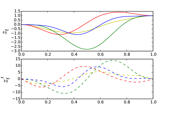
where K(a,b);(a,b)=[Ka;aKa;bKb;aKb;b],subscriptK𝑎𝑏𝑎𝑏matrixsubscriptK𝑎𝑎subscriptK𝑎𝑏subscriptK𝑏𝑎subscriptK𝑏𝑏~{}~{}~{}\textbf{K}_{(a,b);(a,b)}=\begin{bmatrix}\textbf{K}_{a;a}&\textbf{K}_{a;b}\\ \textbf{K}_{b;a}&\textbf{K}_{b;b}\end{bmatrix},~{}~{}~{}and K~t;(a,b)=[K~t;aK~t;b].subscript~K𝑡𝑎𝑏matrixsubscript~K𝑡𝑎subscript~K𝑡𝑏~{}~{}~{}\tilde{\textbf{K}}_{t;(a,b)}=\begin{bmatrix}\tilde{\textbf{K}}_{t;a}&\tilde{\textbf{K}}_{t;b}\end{bmatrix}. It is important to note that both Ka;asubscriptK𝑎𝑎\textbf{K}_{a;a} and K(a,b);(a,b)subscriptK𝑎𝑏𝑎𝑏\textbf{K}_{(a,b);(a,b)} are indeed invertible because the kernel is assumed to be neither degenerate at a𝑎a nor degenerate at b𝑏b given a𝑎a. Hence, the support of (za,za,zb,zb)subscript𝑧𝑎superscriptsubscript𝑧𝑎subscript𝑧𝑏superscriptsubscript𝑧𝑏(z_{a},z_{a}^{\prime},z_{b},z_{b}^{\prime}) is 4superscript4\mathbb{R}^{4}, and any function and derivative values can be used for conditioning. Figure 1 illustrates example independent draws from a conditional derivative Gaussian process.
Refer to caption


Figure 1: Draws from a conditional derivative GP conditioned to start at 00 with derivative 00 and to finish at 1.01.01.0 with derivative 0.00.00.0. The unconditional kernel is the squared exponential kernel with variance 1.01.01.0 and input scale 0.20.20.2.

3.1 String Gaussian Processes on \mathbb{R}

The intuition behind string Gaussian processes on an interval comes from the analogy of collaborative local GP experts we refer to as strings that are connected but independent of each other conditional on some regularity boundary conditions. While each string is tasked with representing local patterns in the data, a string only shares the states of its extremities (value and derivative) with adjacent strings. Our aim is to preserve global smoothness and limit the amount of information shared between strings, thus reducing computational complexity. Furthermore, the conditional independence between strings will allow for distributed inference, greater flexibility and principled nonstationarity construction.

The following theorem at the core of our framework establishes that it is possible to connect together GPs on a partition of an interval I𝐼I, in a manner consistent enough that the newly constructed stochastic object will be a stochastic process on I𝐼I and in a manner restrictive enough that any two connected GPs will share just enough information to ensure that the constructed stochastic process is continuously differentiable (𝒞1superscript𝒞1\mathcal{C}^{1}) on I𝐼I in the L2superscript𝐿2L^{2} sense.

Theorem 2

(String Gaussian process)
Let a0<<ak<<aKsubscripta0subscriptaksubscriptaKa_{0}<\dots<a_{k}<\dots<a_{K}, I=[a0,aK]Isubscripta0subscriptaKI=[a_{0},a_{K}] and let p𝒩(x;μ,Σ)subscriptp𝒩xμΣp_{\mathcal{N}}(x;\mu,\Sigma) be the multivariate Gaussian density with mean vector μμ\mu and covariance matrix ΣΣ\Sigma. Furthermore, let (mk:[ak1,ak])k[1..K](m_{k}:[a_{k-1},a_{k}]\to\mathbb{R})_{k\in[1..K]} be 𝒞1superscript𝒞1\mathcal{C}^{1} functions, and (kk:[ak1,ak]×[ak1,ak])k[1..K](k_{k}:[a_{k-1},a_{k}]\times[a_{k-1},a_{k}]\to\mathbb{R})_{k\in[1..K]} be 𝒞3superscript𝒞3\mathcal{C}^{3} symmetric positive semi-definite functions, neither degenerate at ak1subscriptak1a_{k-1}, nor degenerate at aksubscriptaka_{k} given ak1subscriptak1a_{k-1}.

(A) There exists an 2superscript2\mathbb{R}^{2}-valued stochastic process (SDt)tI,SDt=(zt,zt)subscript𝑆subscript𝐷𝑡𝑡𝐼𝑆subscript𝐷𝑡subscript𝑧𝑡superscriptsubscript𝑧𝑡(SD_{t})_{t\in I},~{}SD_{t}=(z_{t},z_{t}^{\prime}) satisfying the following conditions:

1) The probability density of (SDa0,,SDaK)𝑆subscript𝐷subscript𝑎0𝑆subscript𝐷subscript𝑎𝐾(SD_{a_{0}},\dots,SD_{a_{K}}) reads:

pb(x0,,xK):=k=0Kp𝒩(xk;μkb,Σkb)assignsubscript𝑝𝑏subscript𝑥0subscript𝑥𝐾superscriptsubscriptproduct𝑘0𝐾subscript𝑝𝒩subscript𝑥𝑘subscriptsuperscript𝜇𝑏𝑘superscriptsubscriptΣ𝑘𝑏p_{b}(x_{0},\dots,x_{K}):=\prod_{k=0}^{K}p_{\mathcal{N}}\left(x_{k};\mu^{b}_{k},\Sigma_{k}^{b}\right) (5)
where:Σ0b=Ka0;a01,k>0Σkb=Kak;akkKak;ak1kKak1;ak11kKak;ak1Tk,formulae-sequencewhere:superscriptsubscriptΣ0𝑏subscriptsubscriptKsubscript𝑎0subscript𝑎01for-all𝑘0superscriptsubscriptΣ𝑘𝑏subscriptsubscriptKsubscript𝑎𝑘subscript𝑎𝑘𝑘subscriptsubscriptKsubscript𝑎𝑘subscript𝑎𝑘1𝑘subscriptsuperscriptsubscriptKsubscript𝑎𝑘1subscript𝑎𝑘11𝑘subscriptsuperscriptsubscriptKsubscript𝑎𝑘subscript𝑎𝑘1𝑇𝑘\text{where:}~{}~{}~{}~{}\Sigma_{0}^{b}={}_{1}\textbf{K}_{a_{0};a_{0}},~{}~{}\forall~{}k>0~{}~{}~{}\Sigma_{k}^{b}={}_{k}\textbf{K}_{a_{k};a_{k}}-{}_{k}\textbf{K}_{a_{k};a_{k-1}}~{}{}_{k}\textbf{K}_{a_{k-1};a_{k-1}}^{-1}~{}{}_{k}\textbf{K}_{a_{k};a_{k-1}}^{T}, (6)
μ0b=Ma01,k>0μkb=Makk+Kak;ak1kKak1;ak11k(xk1Mak1k),formulae-sequencesuperscriptsubscript𝜇0𝑏subscriptsubscriptMsubscript𝑎01for-all𝑘0subscriptsuperscript𝜇𝑏𝑘subscriptsubscriptMsubscript𝑎𝑘𝑘subscriptsubscriptKsubscript𝑎𝑘subscript𝑎𝑘1𝑘subscriptsuperscriptsubscriptKsubscript𝑎𝑘1subscript𝑎𝑘11𝑘subscript𝑥𝑘1subscriptsubscriptMsubscript𝑎𝑘1𝑘\mu_{0}^{b}={}_{1}\textbf{M}_{a_{0}},~{}~{}\forall~{}k>0~{}~{}~{}\mu^{b}_{k}={}_{k}\textbf{M}_{a_{k}}+{}_{k}\textbf{K}_{a_{k};a_{k-1}}~{}{}_{k}\textbf{K}_{a_{k-1};a_{k-1}}^{-1}(x_{k-1}-{}_{k}\textbf{M}_{a_{k-1}}), (7)
withKu;vk=[kk(u,v)kky(u,v)kkx(u,v)2kkxy(u,v)],andMuk=[mk(u)dmkdt(u)].formulae-sequencewithsubscriptsubscriptK𝑢𝑣𝑘matrixsubscript𝑘𝑘𝑢𝑣subscript𝑘𝑘𝑦𝑢𝑣subscript𝑘𝑘𝑥𝑢𝑣superscript2subscript𝑘𝑘𝑥𝑦𝑢𝑣andsubscriptsubscriptM𝑢𝑘matrixsubscript𝑚𝑘𝑢𝑑subscript𝑚𝑘𝑑𝑡𝑢\text{with}~{}~{}~{}~{}{}_{k}\textbf{K}_{u;v}=\begin{bmatrix}k_{k}(u,v)&\frac{\partial k_{k}}{\partial y}(u,v)\\ \frac{\partial k_{k}}{\partial x}(u,v)&\frac{\partial^{2}k_{k}}{\partial x\partial y}(u,v)\end{bmatrix},~{}~{}~{}~{}\text{and}~{}~{}~{}~{}{}_{k}\textbf{M}_{u}=\begin{bmatrix}m_{k}(u)\\ \frac{dm_{k}}{dt}(u)\end{bmatrix}.

2) Conditional on (SDak=xk)k[0..K](SD_{a_{k}}=x_{k})_{k\in[0..K]}, the restrictions (SDt)t]ak1,ak[,k[1..K](SD_{t})_{t\in]a_{k-1},a_{k}[},~{}k\in[1..K] are independent conditional derivative Gaussian processes, respectively with unconditional mean function mksubscript𝑚𝑘m_{k} and unconditional covariance function kksubscript𝑘𝑘k_{k} and that are conditioned to take values xk1subscript𝑥𝑘1x_{k-1} and xksubscript𝑥𝑘x_{k} at ak1subscript𝑎𝑘1a_{k-1} and aksubscript𝑎𝑘a_{k} respectively. We refer to (SDt)tIsubscript𝑆subscript𝐷𝑡𝑡𝐼(SD_{t})_{t\in I} as a string derivative Gaussian process, and to its first coordinate (zt)tIsubscriptsubscript𝑧𝑡𝑡𝐼(z_{t})_{t\in I} as a string Gaussian process namely,

(zt)tI𝒮𝒢𝒫({ak},{mk},{kk}).similar-tosubscriptsubscript𝑧𝑡𝑡𝐼𝒮𝒢𝒫subscript𝑎𝑘subscript𝑚𝑘subscript𝑘𝑘(z_{t})_{t\in I}\sim\mathcal{SGP}(\{a_{k}\},\{m_{k}\},\{k_{k}\}).

(B) The string Gaussian process (zt)tIsubscriptsubscript𝑧𝑡𝑡𝐼(z_{t})_{t\in I} defined in (A) is 𝒞1superscript𝒞1\mathcal{C}^{1} in the L2superscript𝐿2L^{2} sense and its L2superscript𝐿2L^{2} derivative is the process (zt)tIsubscriptsuperscriptsubscript𝑧𝑡𝑡𝐼(z_{t}^{\prime})_{t\in I} defined in (A).

Proof  See Appendix C.  
In our collaborative local GP experts analogy, Theorem 2 stipulates that each local expert takes as message from the previous expert its left hand side boundary conditions, conditional on which it generates its right hand side boundary conditions, which it then passes on to the next expert. Conditional on their boundary conditions local experts are independent of each other, and resemble vibrating pieces of string on fixed extremities, hence the name string Gaussian process.

3.2 Pathwise Regularity

Thus far we have dealt with regularity only in the L2superscript𝐿2L^{2} sense. However, we note that a sufficient condition for the process (zt)tIsubscriptsuperscriptsubscript𝑧𝑡𝑡𝐼(z_{t}^{\prime})_{t\in I} in Theorem 2 to be almost surely continuous (i.e. sample paths are continuous with probability 111) and to be the almost sure derivative of the string Gaussian process (zt)tIsubscriptsubscript𝑧𝑡𝑡𝐼(z_{t})_{t\in I}, is that the Gaussian processes on Ik=[ak1,ak]subscript𝐼𝑘subscript𝑎𝑘1subscript𝑎𝑘I_{k}=[a_{k-1},a_{k}] with mean and covariance functions mckak1,aksuperscriptsubscript𝑚𝑐𝑘subscript𝑎𝑘1subscript𝑎𝑘m_{ck}^{a_{k-1},a_{k}} and kckak1,aksubscriptsuperscript𝑘subscript𝑎𝑘1subscript𝑎𝑘𝑐𝑘k^{a_{k-1},a_{k}}_{ck} (as per Equations 3 and 4 with m:=mkassign𝑚subscript𝑚𝑘m:=m_{k} and k:=kkassign𝑘subscript𝑘𝑘k:=k_{k}) are themselves almost surely 𝒞1superscript𝒞1\mathcal{C}^{1} for every boundary condition.666The proof is provided in Appendix D. We refer to (Adler and Taylor, 2011, Theorem 2.5.2) for a sufficient condition under which a 𝒞1superscript𝒞1\mathcal{C}^{1} in L2superscript𝐿2L^{2} Gaussian process is also almost surely 𝒞1superscript𝒞1\mathcal{C}^{1}. As the above question is provably equivalent to that of the almost sure continuity of a Gaussian process (see Adler and Taylor, 2011, p. 30), Kolmogorov’s continuity theorem (see Øksendal, 2003, Theorem 2.2.3) provides a more intuitive, albeit stronger, sufficient condition than that of (Adler and Taylor, 2011, Theorem 2.5.2).

3.3 Illustration

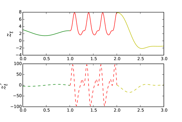
Algorithm 1 illustrates sampling jointly from a string Gaussian process and its derivative on an interval I=[a0,aK]𝐼subscript𝑎0subscript𝑎𝐾I=[a_{0},a_{K}]. We start off by sampling the string boundary conditions (zak,zak)subscript𝑧subscript𝑎𝑘subscriptsuperscript𝑧subscript𝑎𝑘(z_{a_{k}},z^{\prime}_{a_{k}}) sequentially, conditional on which we sample the values of the stochastic process on each string. This we may do in parallel as the strings are independent of each other conditional on boundary conditions. The resulting time complexity is the sum of 𝒪(maxnk3)𝒪superscriptsubscript𝑛𝑘3\mathcal{O}(\max~{}n_{k}^{3}) for sampling values within strings, and 𝒪(n)𝒪𝑛\mathcal{O}(n) for sampling boundary conditions, where the sample size is n=knk𝑛subscript𝑘subscript𝑛𝑘n=\sum_{k}n_{k}. The memory requirement grows as the sum of 𝒪(knk2)𝒪subscript𝑘superscriptsubscript𝑛𝑘2\mathcal{O}(\sum_{k}n_{k}^{2}), required to store conditional covariance matrices of the values within strings, and 𝒪(K)𝒪𝐾\mathcal{O}(K) corresponding to the storage of covariance matrices of boundary conditions. In the special case where strings are all empty, that is inputs and boundary times are the same, the resulting time complexity and memory requirement are 𝒪(n)𝒪𝑛\mathcal{O}(n). Figure 2 illustrates a sample from a string Gaussian process, drawn using this approach.
Refer to caption

Figure 2: Draw from a string GP (zt)subscript𝑧𝑡(z_{t}) with 3 strings and its derivative (zt)superscriptsubscript𝑧𝑡(z_{t}^{\prime}), under squared exponential kernels (green and yellow strings), and the periodic kernel of MacKay (1998) (red string).
Algorithm 1 Simulation of a string derivative Gaussian process
  Inputs: boundary times a0<<aKsubscript𝑎0subscript𝑎𝐾a_{0}<\dots<a_{K}, string times {tjk]ak1,ak[}j[1..nk],k[1..K]\{t_{j}^{k}\in]a_{k-1},a_{k}[\}_{j\in[1..n_{k}],k\in[1..K]}, unconditional mean (resp. covariance) functions mksubscript𝑚𝑘m_{k} (resp. kksubscript𝑘𝑘k_{k})
  Output: {,zak,zak,,ztjk,ztjk,}subscript𝑧subscript𝑎𝑘superscriptsubscript𝑧subscript𝑎𝑘subscript𝑧superscriptsubscript𝑡𝑗𝑘superscriptsubscript𝑧superscriptsubscript𝑡𝑗𝑘\{\dots,z_{a_{k}},z_{a_{k}}^{\prime},\dots,z_{t_{j}^{k}},z_{t_{j}^{k}}^{\prime},\dots\}.
  Step 1: sample the boundary conditions sequentially.
  for k=0𝑘0k=0 to K𝐾K do
     Sample (zak,zak)𝒩(μkb,Σkb)similar-tosubscript𝑧subscript𝑎𝑘superscriptsubscript𝑧subscript𝑎𝑘𝒩superscriptsubscript𝜇𝑘𝑏superscriptsubscriptΣ𝑘𝑏(z_{a_{k}},z_{a_{k}}^{\prime})\sim\mathcal{N}\Big{(}\mu_{k}^{b},\Sigma_{k}^{b}\Big{)}, with μkbsuperscriptsubscript𝜇𝑘𝑏\mu_{k}^{b} and ΣkbsuperscriptsubscriptΣ𝑘𝑏\Sigma_{k}^{b} as per Equations (7) and (6).
  end for
  Step 2: sample the values on each string conditional on the boundary conditions in parallel.
  parfor k=1𝑘1k=1 to K𝐾K do
     Let MuksubscriptsubscriptM𝑢𝑘{}_{k}\textbf{M}_{u} and Ku;vksubscriptsubscriptK𝑢𝑣𝑘{}_{k}\textbf{K}_{u;v} be as in Theorem 2,
Λk=[Kt1k;ak1kKt1k;akkKtnkk;ak1kKtnkk;akk][Kak1;ak1kKak1;akkKak;ak1kKak;akk]1,subscriptΛ𝑘matrixsubscriptsubscriptKsuperscriptsubscript𝑡1𝑘subscript𝑎𝑘1𝑘subscriptsubscriptKsuperscriptsubscript𝑡1𝑘subscript𝑎𝑘𝑘subscriptsubscriptKsuperscriptsubscript𝑡subscript𝑛𝑘𝑘subscript𝑎𝑘1𝑘subscriptsubscriptKsuperscriptsubscript𝑡subscript𝑛𝑘𝑘subscript𝑎𝑘𝑘superscriptmatrixsubscriptsubscriptKsubscript𝑎𝑘1subscript𝑎𝑘1𝑘subscriptsubscriptKsubscript𝑎𝑘1subscript𝑎𝑘𝑘subscriptsubscriptKsubscript𝑎𝑘subscript𝑎𝑘1𝑘subscriptsubscriptKsubscript𝑎𝑘subscript𝑎𝑘𝑘1{}_{k}\Lambda=\begin{bmatrix}{}_{k}\textbf{K}_{t_{1}^{k};a_{k-1}}&{}_{k}\textbf{K}_{t_{1}^{k};a_{k}}\\ \dots&\dots\\ {}_{k}\textbf{K}_{t_{n_{k}}^{k};a_{k-1}}&{}_{k}\textbf{K}_{t_{n_{k}}^{k};a_{k}}\end{bmatrix}\begin{bmatrix}{}_{k}\textbf{K}_{a_{k-1};a_{k-1}}&{}_{k}\textbf{K}_{a_{k-1};a_{k}}\\ {}_{k}\textbf{K}_{a_{k};a_{k-1}}&{}_{k}\textbf{K}_{a_{k};a_{k}}\end{bmatrix}^{-1},
     
μks=[Mt1kkMtnkkk]+Λk[zak1mk(ak1)zak1dmkdt(ak1)zakmk(ak)zakdmkdt(ak)],superscriptsubscript𝜇𝑘𝑠matrixsubscriptsubscriptMsuperscriptsubscript𝑡1𝑘𝑘subscriptsubscriptMsuperscriptsubscript𝑡subscript𝑛𝑘𝑘𝑘subscriptΛ𝑘matrixsubscript𝑧subscript𝑎𝑘1subscript𝑚𝑘subscript𝑎𝑘1superscriptsubscript𝑧subscript𝑎𝑘1𝑑subscript𝑚𝑘𝑑𝑡subscript𝑎𝑘1subscript𝑧subscript𝑎𝑘subscript𝑚𝑘subscript𝑎𝑘superscriptsubscript𝑧subscript𝑎𝑘𝑑subscript𝑚𝑘𝑑𝑡subscript𝑎𝑘\mu_{k}^{s}=\begin{bmatrix}{}_{k}\textbf{M}_{t_{1}^{k}}\\ \dots\\ {}_{k}\textbf{M}_{t_{n_{k}}^{k}}\end{bmatrix}+{}_{k}\Lambda\begin{bmatrix}z_{a_{k-1}}-m_{k}(a_{k-1})\\ z_{a_{k-1}}^{\prime}-\frac{dm_{k}}{dt}(a_{k-1})\\ z_{a_{k}}-m_{k}(a_{k})\\ z_{a_{k}}^{\prime}-\frac{dm_{k}}{dt}(a_{k})\\ \end{bmatrix}, (8)
     
Σks=[Kt1k;t1kkKt1k;tnkkkKtnkk;t1kkKtnkk;tnkkk]Λk[Kt1k;ak1kKt1k;akkKtnkk;ak1kKtnkk;akk]T.superscriptsubscriptΣ𝑘𝑠matrixsubscriptsubscriptKsuperscriptsubscript𝑡1𝑘superscriptsubscript𝑡1𝑘𝑘subscriptsubscriptKsuperscriptsubscript𝑡1𝑘superscriptsubscript𝑡subscript𝑛𝑘𝑘𝑘subscriptsubscriptKsuperscriptsubscript𝑡subscript𝑛𝑘𝑘superscriptsubscript𝑡1𝑘𝑘subscriptsubscriptKsuperscriptsubscript𝑡subscript𝑛𝑘𝑘superscriptsubscript𝑡subscript𝑛𝑘𝑘𝑘subscriptΛ𝑘superscriptmatrixsubscriptsubscriptKsuperscriptsubscript𝑡1𝑘subscript𝑎𝑘1𝑘subscriptsubscriptKsuperscriptsubscript𝑡1𝑘subscript𝑎𝑘𝑘subscriptsubscriptKsuperscriptsubscript𝑡subscript𝑛𝑘𝑘subscript𝑎𝑘1𝑘subscriptsubscriptKsuperscriptsubscript𝑡subscript𝑛𝑘𝑘subscript𝑎𝑘𝑘𝑇\Sigma_{k}^{s}=\begin{bmatrix}{}_{k}\textbf{K}_{t_{1}^{k};t_{1}^{k}}&\dots&{}_{k}\textbf{K}_{t_{1}^{k};t_{n_{k}}^{k}}\\ \dots&\dots&\dots\\ {}_{k}\textbf{K}_{t_{n_{k}}^{k};t_{1}^{k}}&\dots&{}_{k}\textbf{K}_{t_{n_{k}}^{k};t_{n_{k}}^{k}}\end{bmatrix}-{}_{k}\Lambda\begin{bmatrix}{}_{k}\textbf{K}_{t_{1}^{k};a_{k-1}}&{}_{k}\textbf{K}_{t_{1}^{k};a_{k}}\\ \dots&\dots\\ {}_{k}\textbf{K}_{t_{n_{k}}^{k};a_{k-1}}&{}_{k}\textbf{K}_{t_{n_{k}}^{k};a_{k}}\end{bmatrix}^{T}. (9)
     Sample (zt1k,zt1k,ztnkk,ztnkk)𝒩(μks,Σks)similar-tosubscript𝑧superscriptsubscript𝑡1𝑘superscriptsubscript𝑧superscriptsubscript𝑡1𝑘subscript𝑧superscriptsubscript𝑡subscript𝑛𝑘𝑘superscriptsubscript𝑧superscriptsubscript𝑡subscript𝑛𝑘𝑘𝒩superscriptsubscript𝜇𝑘𝑠superscriptsubscriptΣ𝑘𝑠\left(z_{t_{1}^{k}},z_{t_{1}^{k}}^{\prime}\dots,z_{t_{n_{k}}^{k}},z_{t_{n_{k}}^{k}}^{\prime}\right)\sim\mathcal{N}\left(\mu_{k}^{s},\Sigma_{k}^{s}\right).
  end parfor

3.4 String Gaussian Processes on dsuperscript𝑑\mathbb{R}^{d}

So far the input space has been assumed to be an interval. We generalise string GPs to hyper-rectangles in dsuperscript𝑑\mathbb{R}^{d} as stochastic processes of the form:

f(t1,,td)=ϕ(zt11,,ztdd),𝑓subscript𝑡1subscript𝑡𝑑italic-ϕsubscriptsuperscript𝑧1subscript𝑡1subscriptsuperscript𝑧𝑑subscript𝑡𝑑f(t_{1},\dots,t_{d})=\phi\left(z^{1}_{t_{1}},\dots,z^{d}_{t_{d}}\right), (10)

where the link function ϕ:d:italic-ϕsuperscript𝑑\phi:\mathbb{R}^{d}\to\mathbb{R} is a 𝒞1superscript𝒞1\mathcal{C}^{1} function and (ztj)subscriptsuperscript𝑧𝑗𝑡(z^{j}_{t}) are d𝑑d independent (perpendicular-to\perp) latent string Gaussian processes on intervals. We will occasionally refer to string GPs indexed on dsuperscript𝑑\mathbb{R}^{d} with d>1𝑑1d>1 as membrane GPs to avoid any ambiguity. We note that when d=1𝑑1d=1 and when the link function is ϕ(x)=xitalic-ϕ𝑥𝑥\phi(x)=x, we recover string GPs indexed on an interval as previously defined. When the string GPs (ztj)superscriptsubscript𝑧𝑡𝑗(z_{t}^{j}) are a.s. 𝒞1superscript𝒞1\mathcal{C}^{1}, the membrane GP f𝑓f in Equation (10) is also a.s. 𝒞1superscript𝒞1\mathcal{C}^{1}, and the partial derivative with respect to the j𝑗j-th coordinate reads:

ftj(t1,,td)=ztjjϕtj(zt11,,ztdd).𝑓subscript𝑡𝑗subscript𝑡1subscript𝑡𝑑subscriptsuperscript𝑧𝑗subscript𝑡𝑗italic-ϕsubscript𝑡𝑗subscriptsuperscript𝑧1subscript𝑡1subscriptsuperscript𝑧𝑑subscript𝑡𝑑\frac{\partial f}{\partial t_{j}}(t_{1},\dots,t_{d})=z^{j\prime}_{t_{j}}\frac{\partial\phi}{\partial t_{j}}\left(z^{1}_{t_{1}},\dots,z^{d}_{t_{d}}\right). (11)

Thus in high dimensions, string GPs easily allow an explanation of the sensitivity of the learned latent function to inputs.

3.5 Choice of Link Function

Our extension of string GPs to dsuperscript𝑑\mathbb{R}^{d} departs from the standard GP paradigm in that we did not postulate a covariance function on d×dsuperscript𝑑superscript𝑑\mathbb{R}^{d}\times\mathbb{R}^{d} directly. Doing so usually requires using a metric on dsuperscript𝑑\mathbb{R}^{d}, which is often problematic for heterogeneous input dimensions, as it introduces an arbitrary comparison between distances in each input dimension. This problem has been partially addressed by approaches such as Automatic Relevance Determination (ARD) kernels, that allow for a linear rescaling of input dimensions to be learned jointly with kernel hyper-parameters. However, inference under a string GP prior can be thought of as learning a coordinate system in which the latent function f𝑓f resembles the link function ϕitalic-ϕ\phi through non-linear rescaling of input dimensions. In particular, when ϕitalic-ϕ\phi is symmetric, the learned univariate string GPs (being interchangeable in ϕitalic-ϕ\phi) implicitly aim at normalizing input data across dimensions, making string GPs naturally cope with heterogeneous data sets.

An important question arising from our extension is whether or not the link function ϕitalic-ϕ\phi needs to be learned to achieve a flexible functional prior. The flexibility of a string GP as a functional prior depends on both the link function and the covariance structures of the underlying string GP building blocks (ztj)superscriptsubscript𝑧𝑡𝑗(z_{t}^{j}). To address the impact of the choice of ϕitalic-ϕ\phi on flexibility, we constrain the string GP building blocks by restricting them to be independent identically distributed string GPs with one string each (i.e. (ztj)superscriptsubscript𝑧𝑡𝑗(z_{t}^{j}) are i.i.d Gaussian processes). Furthermore, we restrict ourselves to isotropic kernels as they provide a consistent basis for putting the same covariance structure in \mathbb{R} and dsuperscript𝑑\mathbb{R}^{d}. One question we might then ask, for a given link function ϕ0subscriptitalic-ϕ0\phi_{0}, is whether or not an isotropic GP indexed on dsuperscript𝑑\mathbb{R}^{d} with covariance function k𝑘k yields more flexible random surfaces than the stationary string GP f(t1,,td)=ϕ0(zt11,,ztdd)𝑓subscript𝑡1subscript𝑡𝑑subscriptitalic-ϕ0superscriptsubscript𝑧subscript𝑡11superscriptsubscript𝑧subscript𝑡𝑑𝑑f(t_{1},\dots,t_{d})=\phi_{0}(z_{t_{1}}^{1},\dots,z_{t_{d}}^{d}), where (ztjj)superscriptsubscript𝑧subscript𝑡𝑗𝑗(z_{t_{j}}^{j}) are stationary GPs indexed on \mathbb{R} with the same covariance function k𝑘k. If we find a link function ϕ0subscriptitalic-ϕ0\phi_{0} generating more flexible random surfaces than isotropic GP counterparts it would suggest ϕitalic-ϕ\phi need not to be inferred in dimension d>1𝑑1d>1 to be more flexible than any GP using one of the large number of commonly used isotropic kernels, among which squared exponential kernels, rational quadratic kernels, and Matérn kernels to name but a few.

Before discussing whether such a ϕ0subscriptitalic-ϕ0\phi_{0} exists, we need to introduce a rigorous meaning to ‘flexibility’. An intuitive qualitative definition of the flexibility of a stochastic process indexed on dsuperscript𝑑\mathbb{R}^{d} is the ease with which it can generate surfaces with varying shapes from one random sample to another independent one. We recall that the tangent hyperplane to a 𝒞1superscript𝒞1\mathcal{C}^{1} surface yf(x)=0,xdformulae-sequence𝑦𝑓𝑥0𝑥superscript𝑑y-f(x)=0,x\in\mathbb{R}^{d} at some point x0=(t10,,td0)subscript𝑥0subscriptsuperscript𝑡01subscriptsuperscript𝑡0𝑑x_{0}=(t^{0}_{1},\dots,t^{0}_{d}) has equation f(x0)T(xx0)(yf(x0))=0𝑓superscriptsubscript𝑥0𝑇𝑥subscript𝑥0𝑦𝑓subscript𝑥00\nabla f(x_{0})^{T}(x-x_{0})-(y-f(x_{0}))=0 and admits as normal vector (ft1(t10),,ftd(td0),1)𝑓subscript𝑡1subscriptsuperscript𝑡01𝑓subscript𝑡𝑑subscriptsuperscript𝑡0𝑑1(\frac{\partial f}{\partial t_{1}}(t^{0}_{1}),\dots,\frac{\partial f}{\partial t_{d}}(t^{0}_{d}),-1). As tangent hyperplanes approximate a surface locally, a first criterion of flexibility for a random surface yf(x)=0,xdformulae-sequence𝑦𝑓𝑥0𝑥superscript𝑑y-f(x)=0,~{}x\in\mathbb{R}^{d} is the proclivity of the (random) direction of its tangent hyperplane at any point x𝑥x—and hence the proclivity of f(x)𝑓𝑥\nabla f(x)—to vary. This criterion alone, however, does not capture the difference between the local shapes of the random surface at two distinct points. A complementary second criterion of flexibility is the proclivity of the (random) directions of the tangent hyperplanes at any two distinct points x0,x1dsubscript𝑥0subscript𝑥1superscript𝑑x_{0},x_{1}\in\mathbb{R}^{d}—and hence the proclivity of f(x0)𝑓subscript𝑥0\nabla f(x_{0}) and f(x1)𝑓subscript𝑥1\nabla f(x_{1})—to be independent. The first criterion can be measured using the entropy of the gradient at a point, while the second criterion can be measured through the mutual information between the two gradients. The more flexible a stochastic process, the higher the entropy of its gradient at any point, and the lower the mutual information between its gradients at any two distinct points. This is formalised in the definition below.

Definition 3

(Flexibility of stochastic processes)
Let fff and ggg be two real valued, almost surely 𝒞1superscript𝒞1\mathcal{C}^{1} stochastic processes indexed on dsuperscriptd\mathbb{R}^{d}, and whose gradients have a finite entropy everywhere (i.e. x,H(f(x)),H(g(x))<for-allxHfxHgx\forall~{}x,~{}H(\nabla f(x)),H(\nabla g(x))<\infty). We say that fff is more flexible than ggg if the following conditions are met:

1)x,H(f(x))H(g(x)),for-all𝑥𝐻𝑓𝑥𝐻𝑔𝑥~{}\forall~{}x,~{}H(\nabla f(x))\geq H(\nabla g(x)),

2)xy,I(f(x);f(y))I(g(x);g(y))formulae-sequencefor-all𝑥𝑦𝐼𝑓𝑥𝑓𝑦𝐼𝑔𝑥𝑔𝑦~{}\forall~{}x\neq y,~{}I(\nabla f(x);\nabla f(y))\leq I(\nabla g(x);\nabla g(y)),
where H𝐻H is the entropy operator, and I(X;Y)=H(X)+H(Y)H(X,Y)𝐼𝑋𝑌𝐻𝑋𝐻𝑌𝐻𝑋𝑌I(X;Y)=H(X)+H(Y)-H(X,Y) stands for the mutual information between X𝑋X and Y𝑌Y.

The following proposition establishes that the link function ϕs(x1,,xd)=i=jdxjsubscriptitalic-ϕ𝑠subscript𝑥1subscript𝑥𝑑superscriptsubscript𝑖𝑗𝑑subscript𝑥𝑗\phi_{s}\left(x_{1},\dots,x_{d}\right)=\sum_{i=j}^{d}x_{j} yields more flexible stationary string GPs than their isotropic GP counterparts, thereby providing a theoretical underpinning for not inferring ϕitalic-ϕ\phi.

Proposition 4

(Additively separable string GPs are flexible)
Let k(x,y):=ρ(xyL22)assignkxyρsubscriptsuperscriptnormxy2superscriptL2k(x,y):=\rho\left(||x-y||^{2}_{{L^{2}}}\right) be a stationary covariance function generating a.s. 𝒞1superscript𝒞1\mathcal{C}^{1} GP paths indexed on d,d>0superscriptdd0\mathbb{R}^{d},~{}d>0, and ρρ\rho a function that is 𝒞2superscript𝒞2\mathcal{C}^{2} on ]0,+[]0,+\infty[ and continuous at 00. Let ϕs(x1,,xd)=j=1dxjsubscriptϕssubscriptx1subscriptxdsuperscriptsubscriptj1dsubscriptxj\phi_{s}(x_{1},\dots,x_{d})=\sum_{j=1}^{d}x_{j}, let (ztj)tIj,j[1..d](z_{t}^{j})_{t\in I^{j},~{}j\in[1..d]} be independent stationary Gaussian processes with mean 00 and covariance function kkk (where the L2superscriptL2L^{2} norm is on \mathbb{R}), and let f(t1,,td)=ϕs(zt11,,ztdd)fsubscriptt1subscripttdsubscriptϕssuperscriptsubscriptzsubscriptt11superscriptsubscriptzsubscripttddf(t_{1},\dots,t_{d})=\phi_{s}(z_{t_{1}}^{1},\dots,z_{t_{d}}^{d}) be the corresponding stationary string GP. Finally, let ggg be an isotropic Gaussian process indexed on I1××IdsuperscriptI1superscriptIdI^{1}\times\dots\times I^{d} with mean 0 and covariance function kkk (where the L2superscriptL2L^{2} norm is on dsuperscriptd\mathbb{R}^{d}). Then:

1)xI1××Id,H(f(x))=H(g(x))formulae-sequencefor-allxsuperscriptI1superscriptIdHfxHgx~{}\forall~{}x\in I^{1}\times\dots\times I^{d},~{}H(\nabla f(x))=H(\nabla g(x)),
2)xyI1××Id,I(f(x);f(y))I(g(x);g(y))formulae-sequencefor-allxysuperscriptI1superscriptIdIfxfyIgxgy~{}\forall~{}x\neq y\in I^{1}\times\dots\times I^{d},~{}I(\nabla f(x);\nabla f(y))\leq I(\nabla g(x);\nabla g(y)).

Proof  See Appendix E.  
Although the link function need not be inferred in a full nonparametric fashion to yield comparable if not better results than most isotropic kernels used in the standard GP paradigm, for some problems certain link functions might outperform others. In Section 4.2 we analyse a broad family of link functions, and argue that they extend successful anisotropic approaches such as the Automatic Relevance Determination (MacKay (1998)) and the additive kernels of Duvenaud et al. (2011). Moreover, in Section 5 we propose a scalable inference scheme applicable to any link function.

4 Comparison with the Standard GP Paradigm

We have already established that sampling string GPs scales better than sampling GPs under the standard GP paradigm and is amenable to distributed computing. We have also established that stationary additively separable string GPs are more flexible than their isotropic counterparts in the standard GP paradigm. In this section, we provide further theoretical results relating the string GP paradigm to the standard GP paradigm. Firstly we establish that string GPs with link function ϕs(x1,,xd)=i=jdxjsubscriptitalic-ϕ𝑠subscript𝑥1subscript𝑥𝑑superscriptsubscript𝑖𝑗𝑑subscript𝑥𝑗\phi_{s}\left(x_{1},\dots,x_{d}\right)=\sum_{i=j}^{d}x_{j} are GPs. Secondly, we derive the global mean and covariance functions induced by the string GP construction for a variety of link functions. Thirdly, we provide a sense in which the string GP paradigm can be thought of as extending the standard GP paradigm. And finally, we show that the string GP paradigm may serve as a scalable approximation of commonly used stationary kernels.

4.1 Some String GPs are GPs

On one hand we note from Theorem 2 that the restriction of a string GP defined on an interval to the support of the first string—in other words the first local GP expert—is a Gaussian process. On the other hand, the messages passed on from one local GP expert to the next are not necessarily consistent with the unconditional law of the receiving local expert, so that overall a string GP defined on an interval, that is when looked at globally and unconditionally, might not be a Gaussian process. However, the following proposition establishes that some string GPs are indeed Gaussian processes.

Proposition 5

(Additively separable string GPs are GPs)
String Gaussian processes on \mathbb{R} are Gaussian processes. Moreover, string Gaussian processes on dsuperscriptd\mathbb{R}^{d} with link function ϕs(x1,,xd)=j=1dxjsubscriptϕssubscriptx1subscriptxdsuperscriptsubscriptj1dsubscriptxj\phi_{s}(x_{1},\dots,x_{d})=\sum_{j=1}^{d}x_{j} are also Gaussian processes.

Proof  The intuition behind this proof lies in the fact that if X𝑋X is a multivariate Gaussian, and if conditional on X𝑋X, Y𝑌Y is a multivariate Gaussian, providing that the conditional mean of Y𝑌Y depends linearly on X𝑋X and the conditional covariance matrix of Y𝑌Y does not depend on X𝑋X, the vector (X,Y)𝑋𝑌(X,Y) is jointly Gaussian. This will indeed be the case for our collaboration of local GP experts as the boundary conditions picked up by an expert from the previous will not influence the conditional covariance structure of the expert (the conditional covariance strucuture depends only on the partition of the domain, not the values of the boundary conditions) and will affect the mean linearly. See Appendix H for the full proof.  

The above result guarantees that commonly used closed form predictive equations under GP priors are still applicable under some string GP priors, providing the global mean and covariance functions, which we derive in the following section, are available. Proposition 5 also guarantees stability of the corresponding string GPs in the GP family under addition of independent Gaussian noise terms as in regression settings. Moreover, it follows from Proposition 5 that inference techniques developed for Gaussian processes can be readily used under string GP priors. In Section 5 we provide an additional MCMC scheme that exploits the conditional independence between strings to yield greater scalability and distributed inference.

4.2 String GP Kernels and String GP Mean Functions

The approach we have adopted in the construction of string GPs and membrane GPs did not require explicitly postulating a global mean function or covariance function. In Appendix I we derive the global mean and covariance functions that result from our construction. The global covariance function could be used for instance as a stand-alone kernel in any kernel method, for instance GP models under the standard GP paradigm, which would provide a flexible and nonstationary alternative to commonly used kernels that may be used to learn local patterns in data sets—some successful example applications are provided in Section 5. That being said, adopting such a global approach should be limited to small scale problems as the conditional independence structure of string GPs does not easily translate into structures in covariance matrices over string GP values (without derivative information) that can be exploited to speed-up SVD or Cholesky decomposition. Crucially, marginalising out all derivative information in the distribution of derivative string GP values at some inputs would destroy any conditional independence structure, thereby limiting opportunities for scalable inference. In Section 5 we will provide a RJ-MCMC inference scheme that fully exploits the conditional independence structure in string GPs and scales to very large data sets.

4.3 Connection Between Multivariate String GP Kernels and Existing Approaches

We recall that for nd𝑛𝑑n\leq d, the n𝑛n-th order elementary symmetric polynomial (Macdonald (1995)) is given by

e0(x1,,xd):=1,1nden(x1,,xd)=1j1<j2<<jndk=1nxjk.formulae-sequenceassignsubscript𝑒0subscript𝑥1subscript𝑥𝑑1for-all1𝑛𝑑subscript𝑒𝑛subscript𝑥1subscript𝑥𝑑subscript1subscript𝑗1subscript𝑗2subscript𝑗𝑛𝑑superscriptsubscriptproduct𝑘1𝑛subscript𝑥subscript𝑗𝑘\displaystyle e_{0}(x_{1},\dots,x_{d}):=1,~{}~{}~{}\forall 1\leq n\leq d~{}~{}e_{n}(x_{1},\dots,x_{d})=\sum_{1\leq j_{1}<j_{2}<\dots<j_{n}\leq d}~{}~{}\prod_{k=1}^{n}x_{j_{k}}. (12)

As an illustration,

e1(x1,,xd)=j=1dxj=ϕs(x1,,xd),subscript𝑒1subscript𝑥1subscript𝑥𝑑superscriptsubscript𝑗1𝑑subscript𝑥𝑗subscriptitalic-ϕ𝑠subscript𝑥1subscript𝑥𝑑e_{1}(x_{1},\dots,x_{d})=\sum_{j=1}^{d}x_{j}=\phi_{s}(x_{1},\dots,x_{d}),
e2(x1,,xd)=x1x2+x1x3++x1xd++xd1xd,subscript𝑒2subscript𝑥1subscript𝑥𝑑subscript𝑥1subscript𝑥2subscript𝑥1subscript𝑥3subscript𝑥1subscript𝑥𝑑subscript𝑥𝑑1subscript𝑥𝑑e_{2}(x_{1},\dots,x_{d})=x_{1}x_{2}+x_{1}x_{3}+\dots+x_{1}x_{d}+\dots+x_{d-1}x_{d},
\dots
ed(x1,,xd)=j=1dxj=ϕp(x1,,xd).subscript𝑒𝑑subscript𝑥1subscript𝑥𝑑superscriptsubscriptproduct𝑗1𝑑subscript𝑥𝑗subscriptitalic-ϕ𝑝subscript𝑥1subscript𝑥𝑑e_{d}(x_{1},\dots,x_{d})=\prod_{j=1}^{d}x_{j}=\phi_{p}(x_{1},\dots,x_{d}).

Covariance kernels of string GPs, using as link functions elementary symmetric polynomials ensubscript𝑒𝑛e_{n}, extend most popular approaches that combine unidimensional kernels over features for greater flexibility or cheaper design experiments.

The first-order polynomial e1subscript𝑒1e_{1} gives rise to additively separable Gaussian processes, that can be regarded as Bayesian nonparametric generalised additive models (GAM), particularly popular for their interpretability. Moreover, as noted by Durrande et al. (2012), additively separable Gaussian processes are considerably cheaper than alternate transformations in design experiments with high-dimensional input spaces. In addition to the above, additively separable string GPs also allow postulating the existence of local properties in the experimental design process at no extra cost.

The d𝑑d-th order polynomial edsubscript𝑒𝑑e_{d} corresponds to a product of unidimensional kernels, also known as separable kernels. For instance, the popular squared exponential kernel is separable. Separable kernels have been successfully used on large scale inference problems where the inputs form a grid (Saatchi, 2011; Wilson et al., 2014), as they yield covariance matrices that are Kronecker products, leading to maximum likelihood inference in linear time complexity and with linear memory requirement. Separable kernels are often used in conjunction with the automatic relevance determination (ARD) model, to learn the relevance of features through global linear rescaling. However, ARD kernels might be limited in that we might want the relevance of a feature to depend on its value. As an illustration, the market value of a watch can be expected to be a stronger indicator of its owner’s wealth when it is in the top 1 percentile, than when it is in the bottom 1 percentile; the rationale being that possessing a luxurious watch is an indication that one can afford it, whereas possessing a cheap watch might be either an indication of lifestyle or an indication that one cannot afford a more expensive one. Separable string GP kernels extend ARD kernels, in that strings between input dimensions and within an input dimension may have unconditional kernels with different hyper-parameters, and possibly different functional forms, thereby allowing for automatic local relevance determination (ALRD).

More generally, using as link function the n𝑛n-th order elementary symmetric polynomial ensubscript𝑒𝑛e_{n} corresponds to the n𝑛n-th order interaction of the additive kernels of Duvenaud et al. (2011). We also note that the class of link functions ϕ(x1,,xd)=i=1dσiei(x1,,xd)italic-ϕsubscript𝑥1subscript𝑥𝑑superscriptsubscript𝑖1𝑑subscript𝜎𝑖subscript𝑒𝑖subscript𝑥1subscript𝑥𝑑\phi(x_{1},\dots,x_{d})=\sum_{i=1}^{d}\sigma_{i}e_{i}(x_{1},\dots,x_{d}) yield full additive kernels. Duvenaud et al. (2011) noted that such kernels are ‘exceptionally well-suited’ to learn non-local structures in data. String GPs complement additive kernels by allowing them to learn local structures as well.

4.4 String GPs as Extension of the Standard GP Paradigm

The following proposition provides a perspective from which string GPs may be considered as extending Gaussian processes on an interval.

Proposition 6

(Extension of the standard GP paradigm)
Let KKsuperscriptK\in\mathbb{N}^{*}, let I=[a0,aK]Isubscripta0subscriptaKI=[a_{0},a_{K}] and Ik=[ak1,ak]subscriptIksubscriptak1subscriptakI_{k}=[a_{k-1},a_{k}] be intervals with a0<<aKsubscripta0subscriptaKa_{0}<\dots<a_{K}. Furthermore, let m:I:mIm:I\to\mathbb{R} be a 𝒞1superscript𝒞1\mathcal{C}^{1} function, mksubscriptmkm_{k} the restriction of mmm to IksubscriptIkI_{k}, h:I×I:hIIh:I\times I\to\mathbb{R} a 𝒞3superscript𝒞3\mathcal{C}^{3} symmetric positive semi-definite function, and hksubscripthkh_{k} the restriction of hhh to Ik×IksubscriptIksubscriptIkI_{k}\times I_{k}. If

(zt)tI𝒮𝒢𝒫({ak},{mk},{hk}),similar-tosubscriptsubscript𝑧𝑡𝑡𝐼𝒮𝒢𝒫subscript𝑎𝑘subscript𝑚𝑘subscript𝑘(z_{t})_{t\in I}\sim\mathcal{SGP}(\{a_{k}\},\{m_{k}\},\{h_{k}\}),

then

k[1..K],(zt)tIk𝒢𝒫(m,h).\forall~{}k\in[1..K],~{}(z_{t})_{t\in I_{k}}\sim\mathcal{GP}(m,h).

Proof  See Appendix F.  

We refer to the case where unconditional string mean and kernel functions are restrictions of the same functions as in Proposition 6 as uniform string GPs. Although uniform string GPs are not guaranteed to be as much regular at boundary times as their counterparts in the standard GP paradigm, we would like to stress that they may well generate paths that are. In other words, the functional space induced by a uniform string GP on an interval extends the functional space of the GP with the same mean and covariance functions m𝑚m and hh taken globally and unconditionally on the whole interval as in the standard GP paradigm. This allows for (but does not enforce) less regularity at the boundary times. When string GPs are used as functional prior, the posterior mean can in fact have more regularity at the boundary times than the continuous differentiability enforced in the string GP paradigm, providing such regularity is evidenced in the data.

We note from Proposition 6 that when m𝑚m is constant and hh is stationary, the restriction of the uniform string GP (zt)tIsubscriptsubscript𝑧𝑡𝑡𝐼(z_{t})_{t\in I} to any interval whose interior does not contain a boundary time, the largest of which being the intervals [ak1,ak]subscript𝑎𝑘1subscript𝑎𝑘[a_{k-1},a_{k}], is a stationary GP. We refer to such cases as partition stationary string GPs.

4.5 Commonly Used Covariance Functions and their String GP Counterparts

Considering the superior scalability of the string GP paradigm, which we may anticipate from the scalability of sampling string GPs, and which we will confirm empirically in Section 5, a natural question that comes to mind is whether or not kernels commonly used in the standard GP paradigm can be well approximated by string GP kernels, so as to take advantage of the improved scalability of the string GP paradigm. We examine the distortions to commonly used covariance structures resulting from restricting strings to share only 𝒞1superscript𝒞1\mathcal{C}^{1} boundary conditions, and from increasing the number of strings.

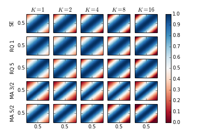
Figure 3 compares some popular stationary kernels on [0,1]×[0,1]0101[0,1]\times[0,1] (first column) to their uniform string GP kernel counterparts with 2, 4, 8 and 16 strings of equal length. The popular kernels considered are the squared exponential kernel (SE), the rational quadratic kernel kRQ(u,v)=(1+2(uv)2α)αsubscript𝑘𝑅𝑄𝑢𝑣superscript12superscript𝑢𝑣2𝛼𝛼k_{RQ}(u,v)=\left(1+\frac{2(u-v)^{2}}{\alpha}\right)^{-\alpha} with α=1𝛼1\alpha=1 (RQ 1) and α=5𝛼5\alpha=5 (RQ 5), the Matérn 3/2 kernel (MA 3/2), and the Matérn 5/2 kernel (MA 5/2), each with output scale (variance) 111 and input scale 0.50.50.5. Firstly, we observe that each of the popular kernels considered coincides with its uniform string GP counterparts regardless of the number of strings, so long as the arguments of the covariance function are less than an input scale apart. Except for the Matérn 3/2, the loss of information induced by restricting strings to share only 𝒞1superscript𝒞1\mathcal{C}^{1} boundary conditions becomes noticeable when the arguments of the covariance function are more than 1.51.51.5 input scales apart, and the effect is amplified as the number of strings increases. As for the Matérn 3/2, no loss of information can been noticed, as further attests Table 1. In fact, this comes as no surprise given that stationary Matérn 3/2 GP are 111-Markov, that is the corresponding derivative Gaussian process is a Markov process so that the vector (zt,zt)subscript𝑧𝑡superscriptsubscript𝑧𝑡(z_{t},z_{t}^{\prime}) contains as much information as all string GP or derivative values prior to t𝑡t (see Doob (1944)). Table 1 provides some statistics on the absolute errors between each of the popular kernels considered and uniform string GP counterparts.
Refer to caption

Figure 3: Commonly used covariance functions on [0,1]×[0,1]0101[0,1]\times[0,1] with the same input and output scales (first column) and their uniform string GP counterparts with K>1𝐾1K>1 strings of equal length.
K=2𝐾2K=2 K=4𝐾4K=4 K=8𝐾8K=8 K=16𝐾16K=16
min avg max min avg max min avg max min avg max
SE 0 0.01 0.13 0 0.02 0.25 0 0.03 0.37 0 0.04 0.44
RQ 1 0 0.01 0.09 0 0.03 0.20 0 0.05 0.37 0 0.07 0.52
RQ 5 0 0.01 0.12 0 0.02 0.24 0 0.04 0.37 0 0.05 0.47
MA 3/2 0 0 0 0 0 0 0 0 0 0 0 0
MA 5/2 0 0.01 0.07 0 0.03 0.15 0 0.05 0.29 0 0.08 0.48
Table 1: Minimum, average, and maximum absolute errors between some commonly used stationary covariance functions on [0,1]×[0,1]0101[0,1]\times[0,1] (with unit variance and input scale 0.5) and their uniform string GP counterparts with K>1𝐾1K>1 strings of equal length.

5 Inference under String and Membrane GP Priors

In this section we move on to developing inference techniques for Bayesian nonparametric inference of latent functions under string GP priors. We begin with marginal likelihood inference in regression problems. We then propose a novel reversible-jump MCMC sampler that enables automatic learning of model complexity (that is the number of different unconditional kernel configurations) from the data, with a time complexity and memory requirement both linear in the number of training inputs.

5.1 Maximum Marginal Likelihood for Small Scale Regression Problems

Firstly, we leverage the fact that additively separable string GPs are Gaussian processes to perform Bayesian nonparametric regressions in the presence of local patterns in the data, using standard Gaussian process techniques (see Rasmussen and Williams, 2006, p.112 §5.4.1). We use as generative model

yi=f(xi)+ϵi,ϵi𝒩(0,σki2),σki2>0,xiI1××Id,yi,ϵiformulae-sequencesubscript𝑦𝑖𝑓subscript𝑥𝑖subscriptitalic-ϵ𝑖subscriptitalic-ϵ𝑖similar-to𝒩0subscriptsuperscript𝜎2subscript𝑘𝑖formulae-sequencesubscriptsuperscript𝜎2subscript𝑘𝑖0formulae-sequencesubscript𝑥𝑖superscript𝐼1superscript𝐼𝑑subscript𝑦𝑖subscriptitalic-ϵ𝑖~{}~{}y_{i}=f(x_{i})+\epsilon_{i},~{}~{}~{}\epsilon_{i}\overset{\text{}}{\sim}\mathcal{N}\left(0,\sigma^{2}_{k_{i}}\right),~{}~{}~{}\sigma^{2}_{k_{i}}>0,~{}~{}~{}x_{i}\in I^{1}\times\dots\times I^{d},~{}~{}~{}y_{i},\epsilon_{i}\in\mathbb{R}

we are given the training data set 𝒟={x~i,y~i}i[1..N],\mathcal{D}=\{\tilde{x}_{i},\tilde{y}_{i}\}_{i\in[1..N]}, and we place a mean-zero additively separable string GP prior on f𝑓f, namely

f(x)=j=1dzx[j]j,(ztj)𝒮𝒢𝒫({akj},{0},{kkj}),j<l,(ztj)(ztl),formulae-sequence𝑓𝑥superscriptsubscript𝑗1𝑑subscriptsuperscript𝑧𝑗𝑥delimited-[]𝑗formulae-sequencesimilar-tosuperscriptsubscript𝑧𝑡𝑗𝒮𝒢𝒫superscriptsubscript𝑎𝑘𝑗0superscriptsubscript𝑘𝑘𝑗formulae-sequencefor-all𝑗𝑙perpendicular-tosuperscriptsubscript𝑧𝑡𝑗superscriptsubscript𝑧𝑡𝑙f(x)=\sum_{j=1}^{d}z^{j}_{x[j]},~{}~{}~{}(z_{t}^{j})\sim\mathcal{SGP}\left(\{a_{k}^{j}\},\{0\},\{k_{k}^{j}\}\right),~{}~{}~{}\forall j<l,~{}(z_{t}^{j})\perp(z_{t}^{l}),

which we assume to be independent of the measurement noise process. Moreover, the noise terms are assumed to be independent, and the noise variance σki2subscriptsuperscript𝜎2subscript𝑘𝑖\sigma^{2}_{k_{i}} affecting f(xi)𝑓subscript𝑥𝑖f(x_{i}) is assumed to be the same for any two inputs whose coordinates lie on the same string intervals. Such a heteroskedastic noise model fits nicely within the string GP paradigm, can be very useful when the dimension of the input space is small, and may be replaced by the typical constant noise variance assumption in high-dimensional input spaces.

Let us define y=(y~1,,y~N)ysubscript~𝑦1subscript~𝑦𝑁\textbf{y}=(\tilde{y}_{1},\dots,\tilde{y}_{N}), X=(x~1,,x~N)Xsubscript~𝑥1subscript~𝑥𝑁\textbf{X}=(\tilde{x}_{1},\dots,\tilde{x}_{N}), f=(f(x~1),,f(x~N))f𝑓subscript~𝑥1𝑓subscript~𝑥𝑁\textbf{f}=(f(\tilde{x}_{1}),\dots,f(\tilde{x}_{N})) and let K¯X;𝐗subscript¯KX𝐗\bar{\textbf{K}}_{\textbf{X};\mathbf{X}} denote the auto-covariance matrix of f (which we have derived in Section 4.2), and let D=diag({σki2})Ddiagsubscriptsuperscript𝜎2subscript𝑘𝑖\textbf{D}=\text{diag}(\{\sigma^{2}_{k_{i}}\}) denote the diagonal matrix of noise variances. It follows that y is a Gaussian vector with mean 𝟎0\bm{0} and auto-covariance matrix Ky:=K¯X;X+DassignsubscriptKysubscript¯KXXD\textbf{K}_{\textbf{y}}:=\bar{\textbf{K}}_{\textbf{X};\textbf{X}}+\textbf{D} and that the log marginal likelihood reads:

logp(y|X,{σki},{θkj},{akj})=12yTKy1y12logdet(Ky)n2log2π.𝑝conditionalyXsubscript𝜎subscript𝑘𝑖superscriptsubscript𝜃𝑘𝑗superscriptsubscript𝑎𝑘𝑗12superscripty𝑇superscriptsubscriptKy1y12detsubscriptKy𝑛22𝜋\displaystyle\log p\left(\textbf{y}\Big{|}\textbf{X},\{\sigma_{k_{i}}\},\{\theta_{k}^{j}\},\{a_{k}^{j}\}\right)=-\frac{1}{2}\textbf{y}^{T}\textbf{K}_{\textbf{y}}^{-1}\textbf{y}-\frac{1}{2}\log{\text{det}\left(\textbf{K}_{\textbf{y}}\right)}-\frac{n}{2}\log{2\pi}. (13)

We obtain estimates of the string measurement noise standard deviations {σ^ki}subscript^𝜎subscript𝑘𝑖\{\hat{\sigma}_{k_{i}}\} and estimates of the string hyper-parameters {θ^kj}superscriptsubscript^𝜃𝑘𝑗\{\hat{\theta}_{k}^{j}\} by maximising the marginal likelihood for a given domain partition {akj}superscriptsubscript𝑎𝑘𝑗\{a_{k}^{j}\}, using gradient-based methods. We deduce the predictive mean and covariance matrix of the latent function values fsuperscriptf\textbf{f}^{*} at test points 𝐗superscript𝐗\mathbf{X}^{*}, from the estimates {θ^kj},{σ^ki}superscriptsubscript^𝜃𝑘𝑗subscript^𝜎subscript𝑘𝑖\{\hat{\theta}_{k}^{j}\},\{\hat{\sigma}_{k_{i}}\} as

E(f|y)=K¯X;XKy1yandcov(f|y)=K¯X;XK¯X;XKy1K¯X;X,formulae-sequenceEconditionalsuperscriptfysubscript¯KsuperscriptXXsuperscriptsubscriptKy1yandcovconditionalsuperscriptfysubscript¯KsuperscriptXsuperscriptXsubscript¯KsuperscriptXXsuperscriptsubscriptKy1subscript¯KXsuperscriptX\text{E}(\textbf{f}^{*}|\textbf{y})=\bar{\textbf{K}}_{\textbf{X}^{*};\textbf{X}}\textbf{K}_{\textbf{y}}^{-1}\textbf{y}~{}~{}~{}~{}\text{and}~{}~{}~{}~{}\text{cov}(\textbf{f}^{*}|\textbf{y})=\bar{\textbf{K}}_{\textbf{X}^{*};\textbf{X}^{*}}-\bar{\textbf{K}}_{\textbf{X}^{*};\textbf{X}}\textbf{K}_{\textbf{y}}^{-1}\bar{\textbf{K}}_{\textbf{X};\textbf{X}^{*}}, (14)

using the fact that (f,y)superscriptfy(\textbf{f}^{*},\textbf{y}) is jointly Gaussian, and that the cross-covariance matrix between fsuperscriptf\textbf{f}^{*} and y is K¯X;Xsubscript¯KsuperscriptXX\bar{\textbf{K}}_{\textbf{X}^{*};\textbf{X}} as the additive measurement noise is assumed to be independent from the latent process f𝑓f.

5.1.1 Remarks

The above analysis and equations still hold when a GP prior is placed on f𝑓f with one of the multivariate string GP kernels derived in Section 4.2 as covariance function.

It is also worth noting from the derivation of string GP kernels in Appendix I that the marginal likelihood Equation (13) is continuously differentiable in the locations of boundary times. Thus, for a given number of boundary times, the positions of the boundary times can be determined as part of the marginal likelihood maximisation. The derivatives of the marginal log-likelihood (Equation 13) with respect to the aforementioned locations {akj}superscriptsubscript𝑎𝑘𝑗\{a_{k}^{j}\} can be determined from the recursions of Appendix I, or approximated numerically by finite differences. The number of boundary times in each input dimension can then be learned by trading off model fit (the maximum marginal log likelihood) and model simplicity (the number of boundary times or model parameters), for instance using information criteria such as AIC and BIC. When the input dimension is large, it might be advantageous to further constrain the hypothesis space of boundary times before using information criteria, for instance by assuming that the number of boundary times is the same in each dimension. An alternative Bayesian nonparametric approach to learning the number of boundary times will be discussed in section 5.4.

This method of inference cannot exploit the structure of string GPs to speed-up inference, and as a result it scales like the standard GP paradigm. In fact, any attempt to marginalize out univariate derivative processes, including in the prior, will inevitably destroy the conditional independence structure. Another perspective to this observation is found by noting from the derivation of global string GP covariance functions in Appendix I that the conditional independence structure does not easily translate in a matrix structure that may be exploited to speed-up matrix inversion, and that marginalizing out terms relating to derivatives processes as in Equation (13) can only make things worse.

5.2 Generic Reversible-Jump MCMC Sampler for Large Scale Inference

More generally, we consider learning a smooth real-valued latent function f𝑓f, defined on a d𝑑d-dimensional hyper-rectangle, under a generative model with likelihood p(𝒟|𝐟,𝐮)𝑝conditional𝒟𝐟𝐮p\left(\mathcal{D}|\mathbf{f},\mathbf{u}\right), where 𝐟𝐟\mathbf{f} denotes values of f𝑓f at training inputs points and 𝐮𝐮\mathbf{u} denotes other likelihood parameters that are not related to f𝑓f. A large class of machine learning problems aiming at inferring a latent function have a likelihood model of this form. Examples include celebrated applications such as nonparametric regression and nonparametric binary classification problems, but also more recent applications such as learning a profitable portfolio generating-function in stochastic portfolio theory (Karatzas and Fernholz (2009)) from the data. In particular, we do not assume that p(𝒟|𝐟,𝐮)𝑝conditional𝒟𝐟𝐮p\left(\mathcal{D}|\mathbf{f},\mathbf{u}\right) factorizes over training inputs. Extensions to likelihood models that depend on the values of multiple latent functions are straight-forward and will be discussed in Section 5.3.

5.2.1 Prior Specification

We place a prior p(𝐮)𝑝𝐮p(\mathbf{u}) on other likelihood parameters. For instance, in regression problems under a Gaussian noise model, 𝐮𝐮\mathbf{u} can be the noise variance and we may choose p(𝐮)𝑝𝐮p(\mathbf{u}) to be the inverse-Gamma distribution for conjugacy. We place a mean-zero string GP prior on f𝑓f

f(x)=ϕ(zx[1]1,,zx[d]d),(ztj)𝒮𝒢𝒫({akj},{0},{kkj}),j<l,(ztj)(ztl).formulae-sequence𝑓𝑥italic-ϕsubscriptsuperscript𝑧1𝑥delimited-[]1subscriptsuperscript𝑧𝑑𝑥delimited-[]𝑑formulae-sequencesimilar-tosuperscriptsubscript𝑧𝑡𝑗𝒮𝒢𝒫superscriptsubscript𝑎𝑘𝑗0superscriptsubscript𝑘𝑘𝑗formulae-sequencefor-all𝑗𝑙perpendicular-tosuperscriptsubscript𝑧𝑡𝑗superscriptsubscript𝑧𝑡𝑙f(x)=\phi\left(z^{1}_{x[1]},\dots,z^{d}_{x[d]}\right),~{}~{}~{}~{}(z_{t}^{j})\sim\mathcal{SGP}\left(\{a_{k}^{j}\},\{0\},\{k_{k}^{j}\}\right),~{}~{}~{}~{}\forall j<l,~{}(z_{t}^{j})\perp(z_{t}^{l}). (15)

As discussed in Section 3.5, the link function ϕitalic-ϕ\phi need not be inferred as the symmetric sum was found to yield a sufficiently flexible functional prior. Nonetheless, in this section we do not impose any restriction on the link function ϕitalic-ϕ\phi other than continuous differentiability. Denoting 𝐳𝐳\mathbf{z} the vector of univariate string GP processes and their derivatives, evaluated at all distinct input coordinate values, we may re-parametrize the likelihood as p(𝒟|𝐳,𝐮)𝑝conditional𝒟𝐳𝐮p\left(\mathcal{D}|\mathbf{z},\mathbf{u}\right), with the understanding that 𝐟𝐟\mathbf{f} can be recovered from 𝐳𝐳\mathbf{z} through the link function ϕitalic-ϕ\phi. To complete our prior specification, we need to discuss the choice of boundary times {akj}superscriptsubscript𝑎𝑘𝑗\{a_{k}^{j}\} and the choice of the corresponding unconditional kernel structures {kkj}superscriptsubscript𝑘𝑘𝑗\{k_{k}^{j}\}. Before doing so, we would like to stress that key requirements of our sampler are that i) it should decouple the need for scalability from the need for flexibility, ii) it should scale linearly with the number of training and test inputs, and iii) the user should be able to express prior views on model complexity/flexibility in an intuitive way, but the sampler should be able to validate or invalidate the prior model complexity from the data. While the motivations for the last two requirements are obvious, the first requirement is motivated by the fact that a massive data set may well be more homogeneous than a much smaller data set.

5.2.2 Scalable Choice of Boundary Times

To motivate our choice of boundary times that achieves great scalability, we first note that the evaluation of the likelihood, which will naturally be needed by the MCMC sampler, will typically have at least linear time complexity and linear memory requirement, as it will require performing computations that use each training sample at least once. Thus, the best we can hope to achieve overall is linear time complexity and linear memory requirement. Second, in MCMC schemes with functional priors, the time complexity and memory requirements for sampling from the posterior

p(𝐟|𝒟)p(𝒟|𝐟)p(𝐟)proportional-to𝑝conditional𝐟𝒟𝑝conditional𝒟𝐟𝑝𝐟p\left(\mathbf{f}|\mathcal{D}\right)\propto p\left(\mathcal{D}|\mathbf{f}\right)p(\mathbf{f})

are often the same as the resource requirements for sampling from the prior p(𝐟)𝑝𝐟p\left(\mathbf{f}\right), as evaluating the model likelihood is rarely the bottleneck. Finally, we note from Algorithm 1 that, when each input coordinate in each dimension is a boundary time, the sampling scheme has time complexity and memory requirement that are linear in the maximum number of unique input coordinates across dimensions, which is at most the number of training samples. In effect, each univariate derivative string GP is sampled in parallel at as many times as there are unique input coordinates in that dimension, before being combined through the link function. In a given input dimension, univariate derivative string GP values are sampled sequentially, one boundary time conditional on the previous. The foregoing sampling operation is very scalable not only asymptotically but also in absolute terms; it merely requires storing and inverting at most as many 2×2222\times 2 matrices as the number of input points. We will evaluate the actual overall time complexity and memory requirement when we discuss our MCMC sampler in greater details. For now, we would like to stress that i) choosing each distinct input coordinate value as a boundary time in the corresponding input dimension before training is a perfectly valid choice, ii) we expect this choice to result in resource requirements that grow linearly with the sample size and iii) in the string GP theory we have developed thus far there is no requirement that two adjacent strings be driven by different kernel hyper-parameters.

5.2.3 Model Complexity Learning as a Change-Point Problem

The remark iii) above pertains to model complexity. In the simplest case, all strings are driven by the same kernel and hyper-parameters as it was the case in Section 4.5, where we discussed how this setup departs from postulating the unconditional string covariance function kkjsuperscriptsubscript𝑘𝑘𝑗k_{k}^{j} globally similarly to the standard GP paradigm. The more distinct unconditional covariance structures there are, the more complex the model is, as it may account for more types of local patterns. Thus, we may identify model complexity to the number of different kernel configurations across input dimensions. In order to learn model complexity, we require that some (but not necessarily all) strings share their kernel configuration.777That is, the functional form of the unconditional kernel kkjsuperscriptsubscript𝑘𝑘𝑗k_{k}^{j} and its hyper-parameters. Moreover, we require kernel membership to be dimension-specific in that two strings in different input dimensions may not explicitly share a kernel configuration in the prior specification, although the posterior distribution over their hyper-parameters might be similar if the data support it.

In each input dimension j𝑗j, kernel membership is defined by a partition of the corresponding domain operated by a (possibly empty) set of change-points,888We would like to stress that change-points do not introduce new input points or boundary times, but solely define a partition of the domain of each input dimension. as illustrated in Figure 4. When there is no change-point as in Figure 4-(a), all strings are driven by the same kernel and hyper-parameters. Each change-point cpjsuperscriptsubscript𝑐𝑝𝑗c_{p}^{j} induces a new kernel configuration θpjsuperscriptsubscript𝜃𝑝𝑗\theta_{p}^{j} that is shared by all strings whose boundary times akjsuperscriptsubscript𝑎𝑘𝑗a_{k}^{j} and ak+1jsuperscriptsubscript𝑎𝑘1𝑗a_{k+1}^{j} both lie in [cpj,cp+1j[[c_{p}^{j},c_{p+1}^{j}[. When one or multiple change-points cpjsuperscriptsubscript𝑐𝑝𝑗c_{p}^{j} occur between two adjacent boundary times as illustrated in Figures 4-(b-d), for instance akjcpjak+1jsuperscriptsubscript𝑎𝑘𝑗superscriptsubscript𝑐𝑝𝑗superscriptsubscript𝑎𝑘1𝑗a_{k}^{j}\leq c_{p}^{j}\leq a_{k+1}^{j}, the kernel configuration of the string defined on [akj,ak+1j]superscriptsubscript𝑎𝑘𝑗superscriptsubscript𝑎𝑘1𝑗[a_{k}^{j},a_{k+1}^{j}] is that of the largest change-point that lies in [akj,ak+1j]superscriptsubscript𝑎𝑘𝑗superscriptsubscript𝑎𝑘1𝑗[a_{k}^{j},a_{k+1}^{j}] (see for instance Figure 4-(d)). For consistency, we denote θ0jsuperscriptsubscript𝜃0𝑗\theta_{0}^{j} the kernel configuration driving the first string in the j𝑗j-th dimension; it also drives strings that come before the first change-point, and all strings when there is no change-point.
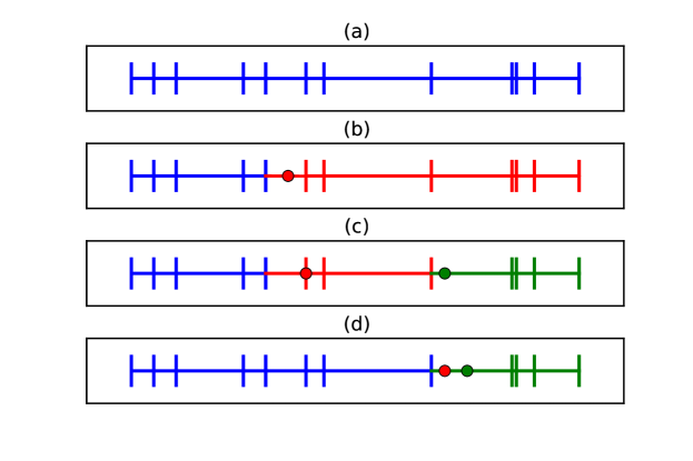
Refer to caption

Figure 4: Effects of domain partition through change-points (coloured circles), on kernel membership. Each vertical bar corresponds to a distinct boundary time akjsuperscriptsubscript𝑎𝑘𝑗a_{k}^{j}. For the same collection of boundary times, we consider four scenarios: (a) no partition, (b) partition of the domain in two by a single change-point that does not coincide with any existing boundary time, (c) partition of the domain in three by two change-points, one of which coincides with an existing boundary time, and (d) partition of the domain in two by two distinct change-points. In each scenario, kernel membership is illustrated by colour-coding. The colour of the interval between two consecutive boundary times akjsuperscriptsubscript𝑎𝑘𝑗a_{k}^{j} and ak+1jsuperscriptsubscript𝑎𝑘1𝑗a_{k+1}^{j} reflects what kernel configuration drives the corresponding string; in particular, the colour of the vertical bar corresponding to boundary time ak+1jsuperscriptsubscript𝑎𝑘1𝑗a_{k+1}^{j} determines what kernel configuration should be used to compute the conditional distribution of the value of the derivative string GP (ztj,ztj)superscriptsubscript𝑧𝑡𝑗superscriptsubscript𝑧𝑡𝑗(z_{t}^{j},z_{t}^{j\prime}) at ak+1jsuperscriptsubscript𝑎𝑘1𝑗a_{k+1}^{j}, given its value at akjsuperscriptsubscript𝑎𝑘𝑗a_{k}^{j}.

To place a prior on model complexity, it suffices to define a joint probability measure on the set of change-points and the corresponding kernel configurations. As kernel configurations are not shared across input dimensions, we choose these priors to be independent across input dimensions. Moreover, {cpj}superscriptsubscript𝑐𝑝𝑗\{c_{p}^{j}\} being a random collection of points on an interval whose number and positions are both random, it is de facto a point process (Daley and Vere-Jones (2008)). To keep the prior specification of change-points uninformative, it is desirable that conditional on the number of change-points, the positions of change-points be i.i.d. uniform on the domain. As for the number of change-points, it is important that the support of its distribution not be bounded, so as to allow for an arbitrarily large model complexity if warranted. The two requirements above are satisfied by a homogeneous Poisson process or HPP (Daley and Vere-Jones (2008)) with constant intensity λjsuperscript𝜆𝑗\lambda^{j}. More precisely, the prior probability measure on ({cpj,θpj},λj)superscriptsubscript𝑐𝑝𝑗superscriptsubscript𝜃𝑝𝑗superscript𝜆𝑗\left(\{c_{p}^{j},\theta_{p}^{j}\},\lambda^{j}\right) is constructed as follows:

{λjΓ(αj,βj),{cpj}|λjHPP(λj)θpj[i]|{cpj},λji.i.dlog𝒩(0,ρj)(j,p)(l,q)θpjθql,,casessimilar-tosuperscript𝜆𝑗Γsuperscript𝛼𝑗superscript𝛽𝑗otherwisesimilar-toconditionalsuperscriptsubscript𝑐𝑝𝑗superscript𝜆𝑗HPPsuperscript𝜆𝑗otherwiseconditionalsuperscriptsubscript𝜃𝑝𝑗delimited-[]𝑖superscriptsubscript𝑐𝑝𝑗superscript𝜆𝑗i.i.dsimilar-to𝒩0superscript𝜌𝑗otherwisefor-all𝑗𝑝𝑙𝑞superscriptsubscript𝜃𝑝𝑗perpendicular-tosuperscriptsubscript𝜃𝑞𝑙otherwise\begin{cases}\lambda^{j}\sim\Gamma(\alpha^{j},\beta^{j}),\\ \{c_{p}^{j}\}\big{|}\lambda^{j}\sim\text{HPP}(\lambda^{j})\\ \theta_{p}^{j}[i]\big{|}\{c_{p}^{j}\},\lambda^{j}~{}~{}\overset{\text{i.i.d}}{\sim}~{}~{}\log\mathcal{N}(0,\rho^{j})\\ \forall(j,p)\neq(l,q)~{}\theta_{p}^{j}\perp\theta_{q}^{l},\end{cases}, (16)

where we choose the Gamma distribution ΓΓ\Gamma as prior on the intensity λjsuperscript𝜆𝑗\lambda^{j} for conjugacy, we assume all kernel hyper-parameters are positive as is often the case in practice,999This may easily be relaxed if needed, for instance by putting normal priors on parameters that may be negative and log-normal priors on positive parameters. the coordinates of the hyper-parameters of a kernel configuration are assumed i.i.d., and kernel hyper-parameters are assumed independent between kernel configurations. Denoting the domain of the j𝑗j-th input [aj,bj]superscript𝑎𝑗superscript𝑏𝑗[a^{j},b^{j}], it follows from applying the laws of total expectation and total variance on Equation (16) that the expected number of change-points in the j𝑗j-th dimension under our prior is

E(#{cpj})=(bjaj)αjβj,E#superscriptsubscript𝑐𝑝𝑗superscript𝑏𝑗superscript𝑎𝑗superscript𝛼𝑗superscript𝛽𝑗\text{E}\left(\#\{c_{p}^{j}\}\right)=\left(b^{j}-a^{j}\right)\frac{\alpha^{j}}{\beta^{j}}, (17)

and the variance of the number of change-points in the j𝑗j-dimension under our prior is

Var(#{cpj})=(bjaj)αjβj(1+(bjaj)βj).Var#superscriptsubscript𝑐𝑝𝑗superscript𝑏𝑗superscript𝑎𝑗superscript𝛼𝑗superscript𝛽𝑗1superscript𝑏𝑗superscript𝑎𝑗superscript𝛽𝑗\text{Var}\left(\#\{c_{p}^{j}\}\right)=\left(b^{j}-a^{j}\right)\frac{\alpha^{j}}{\beta^{j}}\left(1+\frac{\left(b^{j}-a^{j}\right)}{\beta^{j}}\right). (18)

The two equations above may guide the user when setting the parameters αjsuperscript𝛼𝑗\alpha^{j} and βjsuperscript𝛽𝑗\beta^{j}. For instance, these values may be set so that the expected number of change-points in a given input dimension be a fixed fraction of the number of boundary times in that input dimension, and so that the prior variance over the number of change-points be large enough that overall the prior isn’t too informative.

We could have taken a different approach to construct our prior on change-points. In effect, assuming for the sake of the argument that the boundaries of the domain of the j𝑗j-th input, namely ajsuperscript𝑎𝑗a^{j} and bjsuperscript𝑏𝑗b^{j}, are the first and last change-point in that input dimension, we note that the mapping

(,cpj,)(,ppj,):=(,cp+1jcpjbjaj,)superscriptsubscript𝑐𝑝𝑗superscriptsubscript𝑝𝑝𝑗assignsuperscriptsubscript𝑐𝑝1𝑗superscriptsubscript𝑐𝑝𝑗superscript𝑏𝑗superscript𝑎𝑗\left(\dots,c_{p}^{j},\dots\right)\to\left(\dots,p_{p}^{j},\dots\right):=\left(\dots,\frac{c_{p+1}^{j}-c_{p}^{j}}{b^{j}-a^{j}},\dots\right)

defines a bijection between the set of possible change-points in the j𝑗j-th dimension and the set of all discrete probability distributions. Thus, we could have placed as prior on (,ppj,)superscriptsubscript𝑝𝑝𝑗\left(\dots,p_{p}^{j},\dots\right) a Dirichlet process (Ferguson (1973)), a Pitman-Yor process (Pitman and Yor (1997)), more generally normalized completely random measures (Kingman (1967)) or any other probability distribution over partitions. We prefer the point process approach primarily because it provides an easier way of expressing prior belief about model complexity through the expected number of change-points #{cpj}#superscriptsubscript𝑐𝑝𝑗\#\{c_{p}^{j}\}, while remaining uninformative about positions thereof.

One might also be tempted to regard change-points in an input dimension j𝑗j as inducing a partition, not of the domain [aj,bj]superscript𝑎𝑗superscript𝑏𝑗[a^{j},b^{j}], but of the set of boundary times akjsuperscriptsubscript𝑎𝑘𝑗a_{k}^{j} in the same dimension, so that one may define a prior over kernel memberships through a prior over partitions of the set of boundary times. However, this approach would be inconsistent with the aim to learn local patterns in the data if the corresponding random measure is exchangeable. In effect, as boundary times are all input coordinates, local patterns may only arise in the data as a result of adjacent strings sharing kernel configurations. An exchangeable random measure would postulate a priori that two kernel membership assignments that have the same kernel configurations (i.e. the same number of configurations and the same set of hyper-parameters) and the same number of boundary times in each kernel cluster (although not exactly the same boundary times), are equally likely to occur, thereby possibly putting more probability mass on kernel membership assignments that do not respect boundary time adjacency. Unfortunately, exchangeable random measures (among which the Dirichlet process and the Pitman-Yor process) are by far more widely adopted by the machine learning community than non-exchangeable random measures. Thus, this approach might be perceived as overly complex. That being said, as noted by Foti and Williamson (2015), non-exchangeable normalized random measures may be regarded as Poisson point processes (with varying intensity functions) on some augmented spaces, which makes this choice of prior specification somewhat similar, but stronger (that is more informative) than the one we adopt in this paper.

Before deriving the sampling algorithm, it is worth noting that the prior defined in Equation (16) does not admit a density with respect to the same base measure,101010That is the joint prior probability measure is neither discrete, nor continuous. as the number of change-points #{cpj}#superscriptsubscript𝑐𝑝𝑗\#\{c_{p}^{j}\}, and subsequently the number of kernel configurations, may vary from one sample to another. Nevertheless, the joint distribution over the data 𝒟𝒟\mathcal{D} and all other model parameters is well defined and, as we will see later, we may leverage reversible-jump MCMC techniques (Green (1995); Green and Hastie (2009)) to construct a Markov chain that converges to the posterior distribution.

5.2.4 Overall Structure of the MCMC Sampler

To ease notations, we denote 𝒄𝒄\bm{c} the set of all change-points in all input dimensions, we denote 𝒏=(,#{cpj},)d𝒏#superscriptsubscript𝑐𝑝𝑗superscript𝑑\bm{n}=\left(\dots,\#\{c_{p}^{j}\},\dots\right)\in\mathbb{N}^{d} the vector of the numbers of change-points in each input dimension, we denote 𝜽𝜽\bm{\theta} the set of kernel hyper-parameters,111111To simplify the exposition, we assume without loss of generality that each kernel configuration has the same kernel functional form, so that configurations are defined by kernel hyper-parameters. and 𝝆:=(,ρj,)assign𝝆superscript𝜌𝑗\bm{\rho}:=(\dots,\rho^{j},\dots) the vector of variances of the independent log-normal priors on 𝜽𝜽\bm{\theta}. We denote 𝝀:=(,λj,)assign𝝀superscript𝜆𝑗\bm{\lambda}:=(\dots,\lambda^{j},\dots) the vector of change-points intensities, we denote 𝜶:=(,αj,)assign𝜶superscript𝛼𝑗\bm{\alpha}:=(\dots,\alpha^{j},\dots) and 𝜷:=(,βj,)assign𝜷superscript𝛽𝑗\bm{\beta}:=(\dots,\beta^{j},\dots) the vectors of parameters of the Gamma priors we placed on the change-points intensities across the d𝑑d input dimensions, and we recall that 𝐮𝐮\mathbf{u} denotes the vector of likelihood parameters other than the values of the latent function f𝑓f.

We would like to sample from the posterior distribution p(𝐟,𝐟,𝐟,𝐟|𝒟,𝜶,𝜷,𝝆)𝑝𝐟superscript𝐟𝐟conditionalsuperscript𝐟𝒟𝜶𝜷𝝆p(\mathbf{f},\mathbf{f}^{*},\nabla\mathbf{f},\nabla\mathbf{f}^{*}|\mathcal{D},\bm{\alpha},\bm{\beta},\bm{\rho}), where 𝐟𝐟\mathbf{f} and 𝐟superscript𝐟\mathbf{f}^{*} are the vectors of values of the latent function f𝑓f at training and test inputs respectively, and 𝐟,𝐟𝐟superscript𝐟\nabla\mathbf{f},\nabla\mathbf{f}^{*} the corresponding gradients. Denoting 𝐳𝐳\mathbf{z} the vector of univariate string GP processes and their derivatives, evaluated at all distinct training and test input coordinate values, we note that to sample from p(𝐟,𝐟,𝐟,𝐟|𝒟,𝜶,𝜷,𝝆)𝑝𝐟superscript𝐟𝐟conditionalsuperscript𝐟𝒟𝜶𝜷𝝆p(\mathbf{f},\mathbf{f}^{*},\nabla\mathbf{f},\nabla\mathbf{f}^{*}|\mathcal{D},\bm{\alpha},\bm{\beta},\bm{\rho}), it suffices to sample from p(𝐳|𝒟,𝜶,𝜷,𝝆)𝑝conditional𝐳𝒟𝜶𝜷𝝆p(\mathbf{z}|\mathcal{D},\bm{\alpha},\bm{\beta},\bm{\rho}), compute 𝐟𝐟\mathbf{f} and 𝐟superscript𝐟\mathbf{f}^{*} using the link function, and compute the gradients using Equation (11). To sample from p(𝐳|𝒟,𝜶,𝜷,𝝆)𝑝conditional𝐳𝒟𝜶𝜷𝝆p(\mathbf{z}|\mathcal{D},\bm{\alpha},\bm{\beta},\bm{\rho}), we may sample from the target distribution

π(𝒏,𝒄,𝜽,𝝀,𝐳,𝐮):=p(𝒏,𝒄,𝜽,𝝀,𝐳,𝐮|𝒟,𝜶,𝜷,𝝆),assign𝜋𝒏𝒄𝜽𝝀𝐳𝐮𝑝𝒏𝒄𝜽𝝀𝐳conditional𝐮𝒟𝜶𝜷𝝆\pi(\bm{n},\bm{c},\bm{\theta},\bm{\lambda},\mathbf{z},\mathbf{u}):=p(\bm{n},\bm{c},\bm{\theta},\bm{\lambda},\mathbf{z},\mathbf{u}|\mathcal{D},\bm{\alpha},\bm{\beta},\bm{\rho}), (19)

and discard variables that are not of interest. As previously discussed, π𝜋\pi is not absolutely continuous with respect to the same base measure, though we may still decompose it as

π(𝒏,𝒄,𝜽,𝝀,𝐳,𝐮)=1p(𝒟|𝜶,𝜷,𝝆)p(𝒏|𝝀)p(𝝀|𝜶,𝜷)p(𝒄|𝒏)p(𝜽|𝒏,𝝆)p(𝐮)p(𝐳|𝐜,𝜽)p(𝒟|𝐳,𝐮),𝜋𝒏𝒄𝜽𝝀𝐳𝐮1𝑝conditional𝒟𝜶𝜷𝝆𝑝conditional𝒏𝝀𝑝conditional𝝀𝜶𝜷𝑝conditional𝒄𝒏𝑝conditional𝜽𝒏𝝆𝑝𝐮𝑝conditional𝐳𝐜𝜽𝑝conditional𝒟𝐳𝐮\pi(\bm{n},\bm{c},\bm{\theta},\bm{\lambda},\mathbf{z},\mathbf{u})=\color[rgb]{0,1,0}\definecolor[named]{pgfstrokecolor}{rgb}{0,1,0}\frac{1}{p(\mathcal{D}|\bm{\alpha},\bm{\beta},\bm{\rho})}\color[rgb]{0,0,1}\definecolor[named]{pgfstrokecolor}{rgb}{0,0,1}p(\bm{n}|\bm{\lambda})p(\bm{\lambda}|\bm{\alpha},\bm{\beta})\color[rgb]{1,0,0}\definecolor[named]{pgfstrokecolor}{rgb}{1,0,0}p(\bm{c}|\bm{n})p(\bm{\theta}|\bm{n},\bm{\rho})p(\mathbf{u})p(\mathbf{z}|\mathbf{c},\bm{\theta})\color[rgb]{0,0,0}\definecolor[named]{pgfstrokecolor}{rgb}{0,0,0}\pgfsys@color@gray@stroke{0}\pgfsys@color@gray@fill{0}p(\mathcal{D}|\mathbf{z},\mathbf{u}), (20)

where we use the notation p(.)p(.) and p(.|.)p(.|.) to denote probability measures rather than probability density functions or probability mass functions, and where product and scaling operations are usual measure operations. Before proceeding any further, we will introduce a slight re-parametrization of Equation (20) that will improve the inference scheme.

Let 𝐧a=(,#{akj}k,)subscript𝐧𝑎#subscriptsuperscriptsubscript𝑎𝑘𝑗𝑘\mathbf{n}_{a}=(\dots,\#\{a_{k}^{j}\}_{k},\dots) be the vector of the numbers of unique boundary times in all d𝑑d input dimensions. We recall from our prior on f𝑓f that

p(𝐳|𝐜,𝜽)=j=1dp(za0jj,za0jj)k=1𝒏a[j]1p(zakjj,zakjj|zak1jj,zak1jj),𝑝conditional𝐳𝐜𝜽superscriptsubscriptproduct𝑗1𝑑𝑝superscriptsubscript𝑧superscriptsubscript𝑎0𝑗𝑗superscriptsubscript𝑧superscriptsubscript𝑎0𝑗𝑗superscriptsubscriptproduct𝑘1subscript𝒏𝑎delimited-[]𝑗1𝑝superscriptsubscript𝑧superscriptsubscript𝑎𝑘𝑗𝑗conditionalsuperscriptsubscript𝑧superscriptsubscript𝑎𝑘𝑗𝑗superscriptsubscript𝑧superscriptsubscript𝑎𝑘1𝑗𝑗superscriptsubscript𝑧superscriptsubscript𝑎𝑘1𝑗𝑗p(\mathbf{z}|\mathbf{c},\bm{\theta})=\prod_{j=1}^{d}p\left(z_{a_{0}^{j}}^{j},z_{a_{0}^{j}}^{j\prime}\right)\prod_{k=1}^{\bm{n}_{a}[j]-1}p\left(z_{a_{k}^{j}}^{j},z_{a_{k}^{j}}^{j\prime}\Big{|}z_{a_{k-1}^{j}}^{j},z_{a_{k-1}^{j}}^{j\prime}\right), (21)

where each factor in the decomposition above is a bivariate Gaussian density whose mean vector and covariance matrix is obtained from the partitions 𝐜𝐜\mathbf{c}, the kernel hyper-parameters 𝜽𝜽\bm{\theta}, and the kernel membership scheme described in Section 5.2.3 and illustrated in Figure 4, and using Equations (6-7). Let Ku;vkjsubscriptsuperscriptsubscriptK𝑢𝑣𝑗𝑘{}_{k}^{j}\textbf{K}_{u;v} be the unconditional covariance matrix between (zuj,zuj)superscriptsubscript𝑧𝑢𝑗superscriptsubscript𝑧𝑢𝑗\left(z_{u}^{j},z_{u}^{j\prime}\right) and (zvj,zvj)superscriptsubscript𝑧𝑣𝑗superscriptsubscript𝑧𝑣𝑗\left(z_{v}^{j},z_{v}^{j\prime}\right) as per the unconditional kernel structure driving the string defined on the interval [akj,ak+1j[[a_{k}^{j},a_{k+1}^{j}[. Let Σ0j:=Ka0j;a0j0jassignsuperscriptsubscriptΣ0𝑗subscriptsuperscriptsubscriptKsuperscriptsubscript𝑎0𝑗superscriptsubscript𝑎0𝑗𝑗0\Sigma_{0}^{j}:={}_{0}^{j}\textbf{K}_{a_{0}^{j};a_{0}^{j}} be the auto-covariance matrix of (za0jj,za0jj)superscriptsubscript𝑧superscriptsubscript𝑎0𝑗𝑗superscriptsubscript𝑧superscriptsubscript𝑎0𝑗𝑗\left(z_{a_{0}^{j}}^{j},z_{a_{0}^{j}}^{j\prime}\right). Let

Σkj:=Kakj;akjkjKakj;ak1jkjKak1j;ak1j1kjKakj;ak1jTkjassignsuperscriptsubscriptΣ𝑘𝑗subscriptsuperscriptsubscriptKsuperscriptsubscript𝑎𝑘𝑗superscriptsubscript𝑎𝑘𝑗𝑗𝑘subscriptsuperscriptsubscriptKsuperscriptsubscript𝑎𝑘𝑗superscriptsubscript𝑎𝑘1𝑗𝑗𝑘subscriptsuperscriptsuperscriptsubscriptKsuperscriptsubscript𝑎𝑘1𝑗superscriptsubscript𝑎𝑘1𝑗1𝑗𝑘subscriptsuperscriptsuperscriptsubscriptKsuperscriptsubscript𝑎𝑘𝑗superscriptsubscript𝑎𝑘1𝑗𝑇𝑗𝑘\Sigma_{k}^{j}:={}_{k}^{j}\textbf{K}_{a_{k}^{j};a_{k}^{j}}-{}_{k}^{j}\textbf{K}_{a_{k}^{j};a_{k-1}^{j}}{}_{k}^{j}\textbf{K}_{a_{k-1}^{j};a_{k-1}^{j}}^{-1}{}_{k}^{j}\textbf{K}_{a_{k}^{j};a_{k-1}^{j}}^{T}

be the covariance matrix of (zakjj,zakjj)superscriptsubscript𝑧superscriptsubscript𝑎𝑘𝑗𝑗superscriptsubscript𝑧superscriptsubscript𝑎𝑘𝑗𝑗\left(z_{a_{k}^{j}}^{j},z_{a_{k}^{j}}^{j\prime}\right) given (zak1jj,zak1jj)superscriptsubscript𝑧superscriptsubscript𝑎𝑘1𝑗𝑗superscriptsubscript𝑧superscriptsubscript𝑎𝑘1𝑗𝑗\left(z_{a_{k-1}^{j}}^{j},z_{a_{k-1}^{j}}^{j\prime}\right), and

Mkj=Kakj;ak1jkjKak1j;ak1j1kj.superscriptsubscript𝑀𝑘𝑗subscriptsuperscriptsubscriptKsuperscriptsubscript𝑎𝑘𝑗superscriptsubscript𝑎𝑘1𝑗𝑗𝑘subscriptsuperscriptsuperscriptsubscriptKsuperscriptsubscript𝑎𝑘1𝑗superscriptsubscript𝑎𝑘1𝑗1𝑗𝑘M_{k}^{j}={}_{k}^{j}\textbf{K}_{a_{k}^{j};a_{k-1}^{j}}{}_{k}^{j}\textbf{K}_{a_{k-1}^{j};a_{k-1}^{j}}^{-1}.

Finally, let Lkj:=Ukj(Dkj)12assignsuperscriptsubscript𝐿𝑘𝑗superscriptsubscript𝑈𝑘𝑗superscriptsuperscriptsubscript𝐷𝑘𝑗12L_{k}^{j}:=U_{k}^{j}(D_{k}^{j})^{\frac{1}{2}} with Σkj=UkjDkj(Ukj)TsuperscriptsubscriptΣ𝑘𝑗superscriptsubscript𝑈𝑘𝑗superscriptsubscript𝐷𝑘𝑗superscriptsuperscriptsubscript𝑈𝑘𝑗𝑇\Sigma_{k}^{j}=U_{k}^{j}D_{k}^{j}(U_{k}^{j})^{T} the singular value decomposition (SVD) of ΣkjsuperscriptsubscriptΣ𝑘𝑗\Sigma_{k}^{j}. We may choose to represent (za0jj,za0jj)superscriptsubscript𝑧superscriptsubscript𝑎0𝑗𝑗superscriptsubscript𝑧superscriptsubscript𝑎0𝑗𝑗\left(z_{a_{0}^{j}}^{j},z_{a_{0}^{j}}^{j\prime}\right) as

[za0jjza0jj]=L0jx0j,matrixsuperscriptsubscript𝑧superscriptsubscript𝑎0𝑗𝑗superscriptsubscript𝑧superscriptsubscript𝑎0𝑗𝑗superscriptsubscript𝐿0𝑗superscriptsubscript𝑥0𝑗\begin{bmatrix}z_{a_{0}^{j}}^{j}\\ z_{a_{0}^{j}}^{j\prime}\end{bmatrix}=L_{0}^{j}x_{0}^{j}, (22)

and for k>0𝑘0k>0 we may also choose to represent (zakjj,zakjj)superscriptsubscript𝑧superscriptsubscript𝑎𝑘𝑗𝑗superscriptsubscript𝑧superscriptsubscript𝑎𝑘𝑗𝑗\left(z_{a_{k}^{j}}^{j},z_{a_{k}^{j}}^{j\prime}\right) as

[zakjjzakjj]=Mkj[zak1jjzak1jj]+Lkjxkj,matrixsuperscriptsubscript𝑧superscriptsubscript𝑎𝑘𝑗𝑗superscriptsubscript𝑧superscriptsubscript𝑎𝑘𝑗𝑗superscriptsubscript𝑀𝑘𝑗matrixsuperscriptsubscript𝑧superscriptsubscript𝑎𝑘1𝑗𝑗superscriptsubscript𝑧superscriptsubscript𝑎𝑘1𝑗𝑗superscriptsubscript𝐿𝑘𝑗superscriptsubscript𝑥𝑘𝑗\begin{bmatrix}z_{a_{k}^{j}}^{j}\\ z_{a_{k}^{j}}^{j\prime}\end{bmatrix}=M_{k}^{j}\begin{bmatrix}z_{a_{k-1}^{j}}^{j}\\ z_{a_{k-1}^{j}}^{j\prime}\end{bmatrix}+L_{k}^{j}x_{k}^{j}, (23)

where {xkj}superscriptsubscript𝑥𝑘𝑗\{x_{k}^{j}\} are independent bivariate standard normal vectors. Equations (22-23) provide an equivalent representation. In effect, we recall that if Z=M+LX,𝑍𝑀𝐿𝑋Z=M+LX, where X𝒩(0,I)similar-to𝑋𝒩0𝐼X\sim\mathcal{N}(0,I) is a standard multivariate Gaussian, M𝑀M is a real vector, and L𝐿L is a real matrix, then Z𝒩(M,LLT)similar-to𝑍𝒩𝑀𝐿superscript𝐿𝑇Z\sim\mathcal{N}(M,LL^{T}). Equations (22-23) result from applying this result to (za0jj,za0jj)superscriptsubscript𝑧superscriptsubscript𝑎0𝑗𝑗superscriptsubscript𝑧superscriptsubscript𝑎0𝑗𝑗\left(z_{a_{0}^{j}}^{j},z_{a_{0}^{j}}^{j\prime}\right) and (zakjj,zakjj)|(zak1jj,zak1jj)conditionalsuperscriptsubscript𝑧superscriptsubscript𝑎𝑘𝑗𝑗superscriptsubscript𝑧superscriptsubscript𝑎𝑘𝑗𝑗superscriptsubscript𝑧superscriptsubscript𝑎𝑘1𝑗𝑗superscriptsubscript𝑧superscriptsubscript𝑎𝑘1𝑗𝑗\left(z_{a_{k}^{j}}^{j},z_{a_{k}^{j}}^{j\prime}\right)\Big{|}\left(z_{a_{k-1}^{j}}^{j},z_{a_{k-1}^{j}}^{j\prime}\right). We note that at training time, Mkjsuperscriptsubscript𝑀𝑘𝑗M_{k}^{j} and Lkjsuperscriptsubscript𝐿𝑘𝑗L_{k}^{j} only depend on kernel hyper-parameters. Denoting 𝐱𝐱\mathbf{x} the vector of all xkjsuperscriptsubscript𝑥𝑘𝑗x_{k}^{j}, 𝐱𝐱\mathbf{x} is a so-called ‘whitened’ representation of 𝐳𝐳\mathbf{z}, which we prefer for reasons we will discuss shortly. In the whitened representation, the target distribution π𝜋\pi is re-parameterized as

π(𝒏,𝒄,𝜽,𝝀,𝐱,𝐮)=1p(𝒟|𝜶,𝜷,𝝆)p(𝒏|𝝀)p(𝝀|𝜶,𝜷)p(𝒄|𝒏)p(𝜽|𝒏,𝝆)p(𝐮)p(𝐱)p(𝒟|𝐱,𝐜,𝜽,𝐮),𝜋𝒏𝒄𝜽𝝀𝐱𝐮1𝑝conditional𝒟𝜶𝜷𝝆𝑝conditional𝒏𝝀𝑝conditional𝝀𝜶𝜷𝑝conditional𝒄𝒏𝑝conditional𝜽𝒏𝝆𝑝𝐮𝑝𝐱𝑝conditional𝒟𝐱𝐜𝜽𝐮\pi(\bm{n},\bm{c},\bm{\theta},\bm{\lambda},\mathbf{x},\mathbf{u})=\color[rgb]{0,1,0}\definecolor[named]{pgfstrokecolor}{rgb}{0,1,0}\frac{1}{p(\mathcal{D}|\bm{\alpha},\bm{\beta},\bm{\rho})}\color[rgb]{0,0,1}\definecolor[named]{pgfstrokecolor}{rgb}{0,0,1}p(\bm{n}|\bm{\lambda})p(\bm{\lambda}|\bm{\alpha},\bm{\beta})\color[rgb]{1,0,0}\definecolor[named]{pgfstrokecolor}{rgb}{1,0,0}p(\bm{c}|\bm{n})p(\bm{\theta}|\bm{n},\bm{\rho})p(\mathbf{u})p(\mathbf{x})\color[rgb]{0,0,0}\definecolor[named]{pgfstrokecolor}{rgb}{0,0,0}\pgfsys@color@gray@stroke{0}\pgfsys@color@gray@fill{0}p(\mathcal{D}|\mathbf{x},\mathbf{c},\bm{\theta},\mathbf{u}), (24)

where the dependency of the likelihood term on the partitions and the hyper-parameters stems from the need to recover 𝐳𝐳\mathbf{z} and subsequently 𝐟𝐟\mathbf{f} from 𝐱𝐱\mathbf{x} through Equations (22) and (23). The whitened representation Equation (24) has two primary advantages. Firstly, it is robust to ill-conditioning of ΣkjsuperscriptsubscriptΣ𝑘𝑗\Sigma_{k}^{j}, which would typically occur when two adjacent boundary times are too close to each other. In the representation of Equation (20), as one needs to evaluate the density p(𝐳|𝐜,𝜽)𝑝conditional𝐳𝐜𝜽p(\mathbf{z}|\mathbf{c},\bm{\theta}), ill-conditioning of ΣkjsuperscriptsubscriptΣ𝑘𝑗\Sigma_{k}^{j} would result in numerical instabilities. In contrast, in the whitened representation, one needs to evaluate the density p(𝐱)𝑝𝐱p(\mathbf{x}), which is that of i.i.d. standard Gaussians and as such can be evaluated robustly. Moreover, the SVD required to evaluate Lkjsuperscriptsubscript𝐿𝑘𝑗L_{k}^{j} is also robust to ill-conditioning of ΣkjsuperscriptsubscriptΣ𝑘𝑗\Sigma_{k}^{j}, so that Equations (22) and (23) hold and can be robustly evaluated for degenerate Gaussians too. The second advantage of the whitened representation is that it improves mixing by establishing a link between kernel hyper-parameters and the likelihood.

Equation (24) allows us to cast our inference problem as a Bayesian model selection problem under a countable family of models indexed by 𝒏d𝒏superscript𝑑\bm{n}\in\mathbb{N}^{d}, each defined on a different parameter subspace 𝒞𝒏subscript𝒞𝒏\mathcal{C}_{\bm{n}}, with cross-model normalizing constant p(𝒟|𝜶,𝜷,𝝆)𝑝conditional𝒟𝜶𝜷𝝆\color[rgb]{0,1,0}\definecolor[named]{pgfstrokecolor}{rgb}{0,1,0}p(\mathcal{D}|\bm{\alpha},\bm{\beta},\bm{\rho}), model probability driven by p(𝒏|𝝀)p(𝝀|𝜶,𝜷)𝑝conditional𝒏𝝀𝑝conditional𝝀𝜶𝜷\color[rgb]{0,0,1}\definecolor[named]{pgfstrokecolor}{rgb}{0,0,1}p(\bm{n}|\bm{\lambda})p(\bm{\lambda}|\bm{\alpha},\bm{\beta}), model-specific prior p(𝒄|𝒏)p(𝜽|𝒏,𝝆)p(𝐮)p(𝐱)𝑝conditional𝒄𝒏𝑝conditional𝜽𝒏𝝆𝑝𝐮𝑝𝐱\color[rgb]{1,0,0}\definecolor[named]{pgfstrokecolor}{rgb}{1,0,0}p(\bm{c}|\bm{n})p(\bm{\theta}|\bm{n},\bm{\rho})p(\mathbf{u})p(\mathbf{x}), and likelihood p(𝒟|𝐱,𝐜,𝜽,𝐮)𝑝conditional𝒟𝐱𝐜𝜽𝐮p(\mathcal{D}|\mathbf{x},\mathbf{c},\bm{\theta},\mathbf{u}). Critically, it can be seen from Equation (24) that the conditional probability distribution

π(𝒄,𝜽,𝝀,𝐱,𝐮|𝒏)𝜋𝒄𝜽𝝀𝐱conditional𝐮𝒏\pi(\bm{c},\bm{\theta},\bm{\lambda},\mathbf{x},\mathbf{u}|\bm{n})

admits a density with respect to Lebesgue’s measure on 𝒞𝒏subscript𝒞𝒏\mathcal{C}_{\bm{n}}.

Our setup is therefore analogous to that which motivated the seminal paper Green (1995), so that to sample from the posterior π(𝒄,𝜽,𝝀,𝐱,𝐮,𝒏)𝜋𝒄𝜽𝝀𝐱𝐮𝒏\pi(\bm{c},\bm{\theta},\bm{\lambda},\mathbf{x},\mathbf{u},\bm{n}) we may use any Reversible-Jump Metropolis-Hastings (RJ-MH) scheme satisfying detailed balance and dimension-matching as described in section 3.3 of Green (1995). To improve mixing of the Markov chain, we will alternate between a between-models RJ-MH update with target distribution π(𝒏,𝒄,𝜽,𝝀,𝐱,𝐮)𝜋𝒏𝒄𝜽𝝀𝐱𝐮\pi(\bm{n},\bm{c},\bm{\theta},\bm{\lambda},\mathbf{x},\mathbf{u}), and a within-model MCMC-within-Gibbs sampler with target distribution π(𝒄,𝜽,𝝀,𝐱,𝐮|𝒏)𝜋𝒄𝜽𝝀𝐱conditional𝐮𝒏\pi(\bm{c},\bm{\theta},\bm{\lambda},\mathbf{x},\mathbf{u}|\bm{n}). Constructing reversible-jump samplers by alternating between within-model sampling and between-models sampling is standard practice, and it is well-known that doing so yields a Markov chain that converges to the target distribution of interest (see Brooks et al., 2011, p. 50).

In a slight abuse of notation, in the following we might use the notations p(.|.)p(.|.) and p(.)p(.), which we previously used to denote probability measures, to refer to the corresponding probability density functions or probability mass functions.

5.2.5 Within-Model Updates

We recall from Equation (24) that 𝒄,𝜽,𝝀,𝐱,𝐮|𝒟,𝜶,𝜷,𝝆,𝒏𝒄𝜽𝝀𝐱conditional𝐮𝒟𝜶𝜷𝝆𝒏\bm{c},\bm{\theta},\bm{\lambda},\mathbf{x},\mathbf{u}|\mathcal{D},\bm{\alpha},\bm{\beta},\bm{\rho},\bm{n} has probability density function

p(𝒏|𝝀)p(𝝀|𝜶,𝜷)p(𝒄|𝒏)p(𝜽|𝒏,𝝆)p(𝐮)p(𝐱)p(𝒟|𝐱,𝐜,𝜽,𝐮),𝑝conditional𝒏𝝀𝑝conditional𝝀𝜶𝜷𝑝conditional𝒄𝒏𝑝conditional𝜽𝒏𝝆𝑝𝐮𝑝𝐱𝑝conditional𝒟𝐱𝐜𝜽𝐮\color[rgb]{0,0,1}\definecolor[named]{pgfstrokecolor}{rgb}{0,0,1}p(\bm{n}|\bm{\lambda})p(\bm{\lambda}|\bm{\alpha},\bm{\beta})\color[rgb]{1,0,0}\definecolor[named]{pgfstrokecolor}{rgb}{1,0,0}p(\bm{c}|\bm{n})p(\bm{\theta}|\bm{n},\bm{\rho})p(\mathbf{u})p(\mathbf{x})\color[rgb]{0,0,0}\definecolor[named]{pgfstrokecolor}{rgb}{0,0,0}\pgfsys@color@gray@stroke{0}\pgfsys@color@gray@fill{0}p(\mathcal{D}|\mathbf{x},\mathbf{c},\bm{\theta},\mathbf{u}), (25)

up to a normalizing constant.

Updating λ𝜆\bm{\lambda}: By independence of the priors over (𝝀[j],𝒏[j])𝝀delimited-[]𝑗𝒏delimited-[]𝑗(\bm{\lambda}[j],\bm{n}[j]), the distributions 𝝀[j]|𝒏[j]conditional𝝀delimited-[]𝑗𝒏delimited-[]𝑗\bm{\lambda}[j]~{}\big{|}~{}\bm{n}[j] are also independent, so that the updates may be performed in parallel. Moreover, recalling that the prior number of change-points in the j𝑗j-th input dimension is Poisson distributed with intensity 𝝀[j](bjaj)𝝀delimited-[]𝑗superscript𝑏𝑗superscript𝑎𝑗\bm{\lambda}[j]\left(b^{j}-a^{j}\right), and by conjugacy of the Gamma distribution to the Poisson likelihood, it follows that

𝝀[j]|𝒏[j]Γ(𝒏[j]bjaj+𝜶[j],1+𝜷[j]).similar-toconditional𝝀delimited-[]𝑗𝒏delimited-[]𝑗Γ𝒏delimited-[]𝑗superscript𝑏𝑗superscript𝑎𝑗𝜶delimited-[]𝑗1𝜷delimited-[]𝑗\bm{\lambda}[j]~{}\big{|}~{}\bm{n}[j]\sim\Gamma\left(\frac{\bm{n}[j]}{b^{j}-a^{j}}+\bm{\alpha}[j],1+\bm{\beta}[j]\right). (26)

This update step has memory requirement and time complexity both constant in the number of training and test samples.

Updating 𝐮𝐮\mathbf{u}: When the likelihood has additional parameters 𝐮𝐮\mathbf{u}, they may be updated with a Metropolis-Hastings step. Denoting q(𝐮𝐮)𝑞𝐮superscript𝐮q(\mathbf{u}\to\mathbf{u}^{\prime}) the proposal probability density function, the acceptance ratio reads

r𝐮=min(1,p(𝐮)p(𝒟|𝐱,𝐜,𝜽,𝐮)q(𝐮𝐮)p(𝐮)p(𝒟|𝐱,𝐜,𝜽,𝐮)q(𝐮𝐮)).subscript𝑟𝐮1𝑝superscript𝐮𝑝conditional𝒟𝐱𝐜𝜽superscript𝐮𝑞superscript𝐮𝐮𝑝𝐮𝑝conditional𝒟𝐱𝐜𝜽𝐮𝑞𝐮superscript𝐮r_{\mathbf{u}}=\min~{}\left(1,\frac{p(\mathbf{u}^{\prime})p\left(\mathcal{D}|\mathbf{x},\mathbf{c},\bm{\theta},\mathbf{u}^{\prime}\right)q(\mathbf{u}^{\prime}\to\mathbf{u})}{p(\mathbf{u})p\left(\mathcal{D}|\mathbf{x},\mathbf{c},\bm{\theta},\mathbf{u}\right)q(\mathbf{u}\to\mathbf{u}^{\prime})}\right). (27)

In some cases however, it might be possible and more convenient to choose p(𝐮)𝑝𝐮p(\mathbf{u}) to be conjugate to the likelihood p(𝒟|𝐱,𝐜,𝜽,𝐮)𝑝conditional𝒟𝐱𝐜𝜽𝐮p\left(\mathcal{D}|\mathbf{x},\mathbf{c},\bm{\theta},\mathbf{u}\right). For instance, in regression problems under a Gaussian noise model, we may take 𝐮𝐮\mathbf{u} to be the noise variance on which we may place an inverse-gamma prior. Either way, the computational bottleneck of this step is the evaluation of the likelihood p(𝒟|𝐱,𝐜,𝜽,𝐮)𝑝conditional𝒟𝐱𝐜𝜽superscript𝐮p\left(\mathcal{D}|\mathbf{x},\mathbf{c},\bm{\theta},\mathbf{u}^{\prime}\right), which in most cases can be done with a time complexity and memory requirement that are both linear in the number of training samples.

Updating 𝐜𝐜\mathbf{c}: We update the positions of change-points sequentially using the Metropolis-Hastings algorithm, one input dimension j𝑗j at a time, and for each input dimension we proceed in increasing order of change-points. The proposal new position for the change-point cpjsubscriptsuperscript𝑐𝑗𝑝c^{j}_{p} is sampled uniformly at random on the interval ]cjp1,cjp+1[]c^{j}_{p-1},c^{j}_{p+1}[, where cp1jsubscriptsuperscript𝑐𝑗𝑝1c^{j}_{p-1} (resp. cp+1jsubscriptsuperscript𝑐𝑗𝑝1c^{j}_{p+1}) is replaced by ajsuperscript𝑎𝑗a^{j} (resp. bjsuperscript𝑏𝑗b^{j}) for the first (resp. last) change-point. The acceptance probability of this proposal is easily found to be

rcpj=min(1,p(𝒟|𝐱,𝐜,𝜽,𝐮)p(𝒟|𝐱,𝐜,𝜽,𝐮)),subscript𝑟superscriptsubscript𝑐𝑝𝑗1𝑝conditional𝒟𝐱superscript𝐜𝜽𝐮𝑝conditional𝒟𝐱𝐜𝜽𝐮r_{c_{p}^{j}}=\min~{}\left(1,\frac{p\left(\mathcal{D}|\mathbf{x},\mathbf{c}^{\prime},\bm{\theta},\mathbf{u}\right)}{p\left(\mathcal{D}|\mathbf{x},\mathbf{c},\bm{\theta},\mathbf{u}\right)}\right), (28)

where 𝐜superscript𝐜\mathbf{c}^{\prime} is identical to 𝐜𝐜\mathbf{c} except for the change-point to update. This step requires computing the factors {Lkj,Mkj}superscriptsubscript𝐿𝑘𝑗superscriptsubscript𝑀𝑘𝑗\{L_{k}^{j},M_{k}^{j}\} corresponding to inputs in j𝑗j-th dimension whose kernel configuration would change if the proposal were to be accepted, the corresponding vector of derivative string GP values z, and the observation likelihood under the proposal p(𝒟|𝐱,𝐜,𝜽,𝐮)𝑝conditional𝒟𝐱superscript𝐜𝜽𝐮p\left(\mathcal{D}|\mathbf{x},\mathbf{c}^{\prime},\bm{\theta},\mathbf{u}\right). The computational bottleneck of this step is therefore once again the evaluation of the new likelihood p(𝒟|𝐱,𝐜,𝜽,𝐮)𝑝conditional𝒟𝐱superscript𝐜𝜽𝐮p\left(\mathcal{D}|\mathbf{x},\mathbf{c}^{\prime},\bm{\theta},\mathbf{u}\right).

Updating 𝐱𝐱\mathbf{x}: The target conditional density of 𝐱𝐱\mathbf{x} is proportional to

p(x)p(𝒟|𝐱,𝒄,𝜽,𝐮).𝑝x𝑝conditional𝒟𝐱𝒄𝜽𝐮p(\textbf{x})p(\mathcal{D}|\mathbf{x},\bm{c},\bm{\theta},\mathbf{u}). (29)

Recalling that p(𝐱)𝑝𝐱p(\mathbf{x}) is a multivariate standard normal, it follows that the form of Equation (29) makes it convenient to use elliptical slice sampling (Murray et al. (2010)) to sample from the unormalized conditional p(x)p(𝒟|𝐱,𝒄,𝜽,𝐮)𝑝x𝑝conditional𝒟𝐱𝒄𝜽𝐮p(\textbf{x})p(\mathcal{D}|\mathbf{x},\bm{c},\bm{\theta},\mathbf{u}). The two bottlenecks of this update step are sampling a new proposal from p(𝐱)𝑝𝐱p(\mathbf{x}) and evaluating the likelihood p(𝒟|𝐱,𝒄,𝜽,𝐮)𝑝conditional𝒟𝐱𝒄𝜽𝐮p(\mathcal{D}|\mathbf{x},\bm{c},\bm{\theta},\mathbf{u}). Sampling from the multivariate standard normal p(𝐱)𝑝𝐱p(\mathbf{x}) may be massively parallelized, for instance by using GPU Gaussian random number generators. When no parallelism is available, the overall time complexity reads 𝒪(j=1d𝐧a[j])𝒪superscriptsubscript𝑗1𝑑subscript𝐧𝑎delimited-[]𝑗\mathcal{O}\left(\sum_{j=1}^{d}\mathbf{n}_{a}[j]\right), where we recall that 𝐧a[j]subscript𝐧𝑎delimited-[]𝑗\mathbf{n}_{a}[j] denotes the number of distinct training and testing input coordinates in the j𝑗j-th dimension. In particular, if we denote N𝑁N the total number of training and testing d𝑑d-dimensional input samples, then j=1d𝐧a[j]dNsuperscriptsubscript𝑗1𝑑subscript𝐧𝑎delimited-[]𝑗𝑑𝑁\sum_{j=1}^{d}\mathbf{n}_{a}[j]\leq dN, although for many classes of data sets with sparse input values such as images, where each input (single-colour pixel value) may have at most 256256256 distinct values, we might have j=1d𝐧a[j]dNmuch-less-thansuperscriptsubscript𝑗1𝑑subscript𝐧𝑎delimited-[]𝑗𝑑𝑁\sum_{j=1}^{d}\mathbf{n}_{a}[j]\ll dN. As for the memory required to sample from p(𝐱)𝑝𝐱p(\mathbf{x}), it grows proportionally to the size of 𝐱𝐱\mathbf{x}, that is in 𝒪(j=1d𝐧a[j])𝒪superscriptsubscript𝑗1𝑑subscript𝐧𝑎delimited-[]𝑗\mathcal{O}\left(\sum_{j=1}^{d}\mathbf{n}_{a}[j]\right). In regards to the evaluation of the likelihood p(𝒟|𝐱,𝒄,𝜽,𝐮)𝑝conditional𝒟𝐱𝒄𝜽𝐮p(\mathcal{D}|\mathbf{x},\bm{c},\bm{\theta},\mathbf{u}), as previously discussed its resource requirements are application-specific, but it will typically have time complexity that grows in 𝒪(N)𝒪𝑁\mathcal{O}\left(N\right) and memory requirement that grows in 𝒪(dN)𝒪𝑑𝑁\mathcal{O}\left(dN\right). For instance, the foregoing resource requirements always hold for i.i.d. observation models such as in nonparametric regression and nonparametric classification problems.

Updating θ𝜃\bm{\theta}: We note from Equation (25) that the conditional distribution of 𝜽𝜽\bm{\theta} given everything else has unormalized density

p(𝜽|𝒏,𝝆)p(𝒟|𝐱,𝒄,𝜽,𝐮),𝑝conditional𝜽𝒏𝝆𝑝conditional𝒟𝐱𝒄𝜽𝐮p(\bm{\theta}|\bm{n},\bm{\rho})p(\mathcal{D}|\mathbf{x},\bm{c},\bm{\theta},\mathbf{u}), (30)

which we may choose to represent as

p(log𝜽|𝒏,𝝆)p(𝒟|𝐱,𝒄,log𝜽,𝐮).𝑝conditional𝜽𝒏𝝆𝑝conditional𝒟𝐱𝒄𝜽𝐮p(\log\bm{\theta}|\bm{n},\bm{\rho})p(\mathcal{D}|\mathbf{x},\bm{c},\log\bm{\theta},\mathbf{u}). (31)

As we have put independent log-normal priors on the coordinates of 𝜽𝜽\bm{\theta} (see Equation 16), we may once again use elliptical slice sampling to sample from log𝜽𝜽\log\bm{\theta} before taking the exponential. The time complexity of generating a new sample from p(log𝜽|𝒏,𝝆)𝑝conditional𝜽𝒏𝝆p(\log\bm{\theta}|\bm{n},\bm{\rho}) will typically be at most linear in the total number of distinct kernel hyper-parameters. Overall, the bottleneck of this update is the evaluation of the likelihood p(𝒟|𝐱,𝒄,log𝜽,𝐮)𝑝conditional𝒟𝐱𝒄𝜽𝐮p(\mathcal{D}|\mathbf{x},\bm{c},\log\bm{\theta},\mathbf{u}). In this update, the latter operation requires recomputing the factors Mkjsuperscriptsubscript𝑀𝑘𝑗M_{k}^{j} and Lkjsuperscriptsubscript𝐿𝑘𝑗L_{k}^{j} of Equations (22) and (23), which requires computing and taking the SVD of unrelated 2×2222\times 2 matrices, computations we may perform in parallel. Once the foregoing factors have been computed, we evaluate 𝐳𝐳\mathbf{z}, the derivative string GP values at boundary times, parallelizing over input dimensions, and running a sequential update within an input dimension using Equations (22) and (23). Updating 𝐳𝐳\mathbf{z} therefore has time complexity that is, in the worst case where no distributed computing is available, 𝒪(dN)𝒪𝑑𝑁\mathcal{O}\left(dN\right), and 𝒪(N)𝒪𝑁\mathcal{O}\left(N\right) when there are up to d𝑑d computing cores. The foregoing time complexity will also be that of this update step, unless the observation likelihood is more expensive to evaluate. The memory requirement, as in previous updates, is 𝒪(dN)𝒪𝑑𝑁\mathcal{O}\left(dN\right).

Overall resource requirement: To summarize previous remarks, the overall computational bottleneck of a within-model iteration is the evaluation of the likelihood p(𝒟|𝐱,𝒄,𝜽,𝐮)𝑝conditional𝒟𝐱𝒄𝜽𝐮p(\mathcal{D}|\mathbf{x},\bm{c},\bm{\theta},\mathbf{u}). For i.i.d. observation models such as classification and regression problems for instance, the corresponding time complexity grows in 𝒪(N)𝒪𝑁\mathcal{O}(N) when d𝑑d computing cores are available, or 𝒪(dN)𝒪𝑑𝑁\mathcal{O}(dN) otherwise, and the memory requirement grows in 𝒪(dN)𝒪𝑑𝑁\mathcal{O}(dN).

5.2.6 Between-Models Updates

Our reversible-jump Metropolis-Hastings update proceeds as follows. We choose an input dimension, say j𝑗j, uniformly at random. If j𝑗j has no change-points, that is 𝐧[j]=0𝐧delimited-[]𝑗0\mathbf{n}[j]=0, we randomly choose between not doing anything, and adding a change-point, each outcome having the same probability. If 𝐧[j]>0𝐧delimited-[]𝑗0\mathbf{n}[j]>0, we either do nothing, add a change-point, or delete a change-point, each outcome having the same probability of occurrence.

Whenever we choose not to do anything, the acceptance ratio is easily found to be one:

rj0=1.subscript𝑟𝑗01r_{j0}=1. (32)

Whenever we choose to add a change-point, we sample the position cjsubscriptsuperscript𝑐𝑗c^{j}_{*} of the proposal new change-point uniformly at random on the domain [aj,bj]superscript𝑎𝑗superscript𝑏𝑗[a^{j},b^{j}] of the j𝑗j-th input dimension. This proposal will almost surely break an existing kernel membership cluster, say the p𝑝p-th, into two; that is cpj<cj<cp+1jsubscriptsuperscript𝑐𝑗𝑝subscriptsuperscript𝑐𝑗superscriptsubscript𝑐𝑝1𝑗c^{j}_{p}<c^{j}_{*}<c_{p+1}^{j} where we may have aj=cpjsuperscript𝑎𝑗subscriptsuperscript𝑐𝑗𝑝a^{j}=c^{j}_{p} and/or bj=cp+1jsuperscript𝑏𝑗subscriptsuperscript𝑐𝑗𝑝1b^{j}=c^{j}_{p+1}. In the event cjsubscriptsuperscript𝑐𝑗c^{j}_{*} coincides with an existing change-point, which should happen with probability 00, we do nothing. When adding a change-point, we sample a new vector of hyper-parameters θjsuperscriptsubscript𝜃𝑗\theta_{*}^{j} from the log-normal prior of Equation (16), and we propose as hyper-parameters for the tentative new clusters [cpj,cj[[c^{j}_{p},c^{j}_{*}[ and [cj,cp+1j[[c^{j}_{*},c^{j}_{p+1}[ the vectors θadd-leftjsuperscriptsubscript𝜃add-left𝑗\theta_{\text{add-left}}^{j} and θadd-rightjsuperscriptsubscript𝜃add-right𝑗\theta_{\text{add-right}}^{j} defined as

logθadd-leftj:=cos(α)logθpjsin(α)logθjassignsuperscriptsubscript𝜃add-left𝑗𝛼superscriptsubscript𝜃𝑝𝑗𝛼superscriptsubscript𝜃𝑗\log\theta_{\text{add-left}}^{j}:=\cos(\alpha)\log\theta_{p}^{j}-\sin(\alpha)\log\theta_{*}^{j} (33)

and

logθadd-rightj:=sin(α)logθpj+cos(α)logθjassignsuperscriptsubscript𝜃add-right𝑗𝛼superscriptsubscript𝜃𝑝𝑗𝛼superscriptsubscript𝜃𝑗\log\theta_{\text{add-right}}^{j}:=\sin(\alpha)\log\theta_{p}^{j}+\cos(\alpha)\log\theta_{*}^{j} (34)

respectively, where α[0,π2]𝛼0𝜋2\alpha\in[0,\frac{\pi}{2}] and θpjsuperscriptsubscript𝜃𝑝𝑗\theta_{p}^{j} is the vector of hyper-parameters currently driving the kernel membership defined by the cluster [cpj,cp+1j[[c^{j}_{p},c_{p+1}^{j}[. We note that if θpjsuperscriptsubscript𝜃𝑝𝑗\theta_{p}^{j} is distributed as per the prior in Equation (16) then θadd-leftjsuperscriptsubscript𝜃add-left𝑗\theta_{\text{add-left}}^{j} and θadd-rightjsuperscriptsubscript𝜃add-right𝑗\theta_{\text{add-right}}^{j} are i.i.d. distributed as per the foregoing prior. More generally, this elliptical transformation determines the extent to which the new proposal kernel configurations should deviate from the current configuration θpjsuperscriptsubscript𝜃𝑝𝑗\theta_{p}^{j}. α𝛼\alpha is restricted to [0,π2]0𝜋2[0,\frac{\pi}{2}] so as to give a positive weight the the current vector of hyper-parameters θpjsuperscriptsubscript𝜃𝑝𝑗\theta_{p}^{j}. When α=0𝛼0\alpha=0, the left hand-side cluster [cpj,cj[[c^{j}_{p},c^{j}_{*}[ will fully exploit the current kernel configuration, while the right hand-side cluster [cj,cp+1j[[c^{j}_{*},c^{j}_{p+1}[ will use the prior to explore a new set of hyper-parameters. When α=π2𝛼𝜋2\alpha=\frac{\pi}{2} the reverse occurs. To preserve symmetry between the left and right hand-side kernel configurations, we choose

α=π4.𝛼𝜋4\alpha=\frac{\pi}{4}. (35)

Whenever we choose to delete a change-point, we choose an existing change-point uniformly at random, say cpjsubscriptsuperscript𝑐𝑗𝑝c^{j}_{p}. Deleting cpjsubscriptsuperscript𝑐𝑗𝑝c^{j}_{p}, would merge the clusters [cp1j,cpj[[c^{j}_{p-1},c^{j}_{p}[ and [cpj,cp+1j[[c^{j}_{p},c^{j}_{p+1}[, where we may have aj=cp1jsuperscript𝑎𝑗subscriptsuperscript𝑐𝑗𝑝1a^{j}=c^{j}_{p-1} and/or bj=cp+1jsuperscript𝑏𝑗subscriptsuperscript𝑐𝑗𝑝1b^{j}=c^{j}_{p+1}. We propose as vector of hyper-parameters for the tentative merged cluster [cp1j,cp+1j[[c^{j}_{p-1},c^{j}_{p+1}[ the vector θdel-mergedjsuperscriptsubscript𝜃del-merged𝑗\theta_{\text{del-merged}}^{j} satisfying:

logθdel-mergedj=cos(α)logθp1j+sin(α)logθpj,superscriptsubscript𝜃del-merged𝑗𝛼subscriptsuperscript𝜃𝑗𝑝1𝛼subscriptsuperscript𝜃𝑗𝑝\log\theta_{\text{del-merged}}^{j}=\cos(\alpha)\log\theta^{j}_{p-1}+\sin(\alpha)\log\theta^{j}_{p}, (36)

which together with

logθdel-*j=sin(α)logθp1j+cos(α)logθpj,superscriptsubscript𝜃del-*𝑗𝛼subscriptsuperscript𝜃𝑗𝑝1𝛼subscriptsuperscript𝜃𝑗𝑝\log\theta_{\text{del-*}}^{j}=-\sin(\alpha)\log\theta^{j}_{p-1}+\cos(\alpha)\log\theta^{j}_{p}, (37)

constitute the inverse of the transformation defined by Equations (33) and (34).

Whenever a proposal to add or delete a change-point occurs, the factors Lkjsuperscriptsubscript𝐿𝑘𝑗L_{k}^{j} and Mkjsuperscriptsubscript𝑀𝑘𝑗M_{k}^{j} that would be affected by the change in kernel membership structure are recomputed, and so are the affected coordinates of 𝐳𝐳\mathbf{z}.

This scheme satisfies the reversibility and dimension-matching requirements of Green (1995). Moreover, the absolute value of the Jacobian of the mapping

(logθpj,logθj)(logθadd-leftj,logθadd-rightj)superscriptsubscript𝜃𝑝𝑗superscriptsubscript𝜃𝑗superscriptsubscript𝜃add-left𝑗superscriptsubscript𝜃add-right𝑗\left(\log\theta_{p}^{j},~{}\log\theta_{*}^{j}\right)\to\left(\log\theta_{\text{add-left}}^{j},~{}\log\theta_{\text{add-right}}^{j}\right)

of the move to add a change-point in [cpj,cp+1j[[c^{j}_{p},c^{j}_{p+1}[ reads

|(logθadd-leftj,logθadd-rightj)(logθpj,logθj)|=1.superscriptsubscript𝜃add-left𝑗superscriptsubscript𝜃add-right𝑗superscriptsubscript𝜃𝑝𝑗superscriptsubscript𝜃𝑗1\left|\frac{\partial\left(\log\theta_{\text{add-left}}^{j},\log\theta_{\text{add-right}}^{j}\right)}{\partial\left(\log\theta_{p}^{j},\log\theta_{*}^{j}\right)}\right|=1. (38)

Similarly, the absolute value of the Jacobian of the mapping corresponding to a move to delete change-point cpjsubscriptsuperscript𝑐𝑗𝑝c^{j}_{p}, namely

(logθp1j,logθpj)(logθdel-mergedj,logθdel-*j),subscriptsuperscript𝜃𝑗𝑝1subscriptsuperscript𝜃𝑗𝑝superscriptsubscript𝜃del-merged𝑗superscriptsubscript𝜃del-*𝑗\left(\log\theta^{j}_{p-1},~{}\log\theta^{j}_{p}\right)\to\left(\log\theta_{\text{del-merged}}^{j},~{}\log\theta_{\text{del-*}}^{j}\right),

reads:

|(logθdel-mergedj,logθdel-*j)(logθp1j,logθpj)|=1.superscriptsubscript𝜃del-merged𝑗superscriptsubscript𝜃del-*𝑗subscriptsuperscript𝜃𝑗𝑝1subscriptsuperscript𝜃𝑗𝑝1\Bigg{|}\frac{\partial\left(\log\theta_{\text{del-merged}}^{j},\log\theta_{\text{del-*}}^{j}\right)}{\partial\left(\log\theta^{j}_{p-1},\log\theta^{j}_{p}\right)}\Bigg{|}=1. (39)

Applying the standard result Equation (8) of Green (1995), the acceptance ratio of the move to add a change-point is found to be

rj+=min(1,p(𝒟|𝐱,𝒄+,𝜽+,𝐮)p(𝒟|𝐱,𝒄,𝜽,𝐮)𝝀[j](bjaj)1+𝐧[j]plogθj(logθadd-leftj)plogθj(logθadd-rightj)plogθj(logθpj)plogθj(logθj))subscript𝑟limit-from𝑗1𝑝conditional𝒟𝐱subscript𝒄subscript𝜽𝐮𝑝conditional𝒟𝐱𝒄𝜽𝐮𝝀delimited-[]𝑗superscript𝑏𝑗superscript𝑎𝑗1𝐧delimited-[]𝑗subscript𝑝superscript𝜃𝑗subscriptsuperscript𝜃𝑗add-leftsubscript𝑝superscript𝜃𝑗subscriptsuperscript𝜃𝑗add-rightsubscript𝑝superscript𝜃𝑗subscriptsuperscript𝜃𝑗𝑝subscript𝑝superscript𝜃𝑗subscriptsuperscript𝜃𝑗\displaystyle r_{j+}=\min\left(1,{\color[rgb]{0,0.88,0}\definecolor[named]{pgfstrokecolor}{rgb}{0,0.88,0}\pgfsys@color@cmyk@stroke{0.91}{0}{0.88}{0.12}\pgfsys@color@cmyk@fill{0.91}{0}{0.88}{0.12}{\frac{p(\mathcal{D}|\mathbf{x},\bm{c}_{+},\bm{\theta}_{+},\mathbf{u})}{p(\mathcal{D}|\mathbf{x},\bm{c},\bm{\theta},\mathbf{u})}}}{\color[rgb]{1,0,0}\definecolor[named]{pgfstrokecolor}{rgb}{1,0,0}{\frac{\bm{\lambda}[j]\left(b^{j}-a^{j}\right)}{1+\mathbf{n}[j]}}}{\color[rgb]{0,0,1}\definecolor[named]{pgfstrokecolor}{rgb}{0,0,1}{\frac{p_{\log\theta^{j}}\left(\log\theta^{j}_{\text{add-left}}\right)p_{\log\theta^{j}}\left(\log\theta^{j}_{\text{add-right}}\right)}{p_{\log\theta^{j}}\left(\log\theta^{j}_{p}\right)p_{\log\theta^{j}}\left(\log\theta^{j}_{*}\right)}}}\right) (40)

where plogθjsubscript𝑝superscript𝜃𝑗p_{\log\theta^{j}} is the prior over log hyper-parameters in the j𝑗j-th input dimension (as per the prior specification Equation 16), which we recall is i.i.d. centred Gaussian with variance 𝝆[j]𝝆delimited-[]𝑗\bm{\rho}[j], and 𝒄+subscript𝒄\bm{c}_{+} and 𝜽+subscript𝜽\bm{\theta}_{+} denote the proposal new vector of change-points and the corresponding vector of hyper-parameters. The three coloured terms in the acceptance probability are very intuitive. The green term p(𝒟|𝐱,𝒄+,𝜽+,𝐮)p(𝒟|𝐱,𝒄,𝜽,𝐮)𝑝conditional𝒟𝐱subscript𝒄subscript𝜽𝐮𝑝conditional𝒟𝐱𝒄𝜽𝐮{\color[rgb]{0,0.88,0}\definecolor[named]{pgfstrokecolor}{rgb}{0,0.88,0}\pgfsys@color@cmyk@stroke{0.91}{0}{0.88}{0.12}\pgfsys@color@cmyk@fill{0.91}{0}{0.88}{0.12}{\frac{p(\mathcal{D}|\mathbf{x},\bm{c}_{+},\bm{\theta}_{+},\mathbf{u})}{p(\mathcal{D}|\mathbf{x},\bm{c},\bm{\theta},\mathbf{u})}}} represents the fit improvement that would occur if the new proposal is accepted. In the red term 𝝀[j](bjaj)1+𝐧[j]𝝀delimited-[]𝑗superscript𝑏𝑗superscript𝑎𝑗1𝐧delimited-[]𝑗{\color[rgb]{1,0,0}\definecolor[named]{pgfstrokecolor}{rgb}{1,0,0}{\frac{\bm{\lambda}[j]\left(b^{j}-a^{j}\right)}{1+\mathbf{n}[j]}}}, 𝝀[j](bjaj)𝝀delimited-[]𝑗superscript𝑏𝑗superscript𝑎𝑗{\color[rgb]{1,0,0}\definecolor[named]{pgfstrokecolor}{rgb}{1,0,0}{\bm{\lambda}[j]\left(b^{j}-a^{j}\right)}} represents the average number of change-points in the j𝑗j-th input dimension as per the HPP prior, while 1+𝐧[j]1𝐧delimited-[]𝑗{\color[rgb]{1,0,0}\definecolor[named]{pgfstrokecolor}{rgb}{1,0,0}{1+\mathbf{n}[j]}} corresponds to the proposal new number of change-points in the j𝑗j-th dimension, so that the whole red term acts as a complexity regulariser. Finally, the blue term plogθj(logθadd-leftj)plogθj(logθadd-rightj)plogθj(logθpj)plogθj(logθj)subscript𝑝superscript𝜃𝑗subscriptsuperscript𝜃𝑗add-leftsubscript𝑝superscript𝜃𝑗subscriptsuperscript𝜃𝑗add-rightsubscript𝑝superscript𝜃𝑗subscriptsuperscript𝜃𝑗𝑝subscript𝑝superscript𝜃𝑗subscriptsuperscript𝜃𝑗{\color[rgb]{0,0,1}\definecolor[named]{pgfstrokecolor}{rgb}{0,0,1}{\frac{p_{\log\theta^{j}}\left(\log\theta^{j}_{\text{add-left}}\right)p_{\log\theta^{j}}\left(\log\theta^{j}_{\text{add-right}}\right)}{p_{\log\theta^{j}}\left(\log\theta^{j}_{p}\right)p_{\log\theta^{j}}\left(\log\theta^{j}_{*}\right)}}} plays the role of hyper-parameters regulariser.

Similarly, the acceptance ratio of the move to delete change-point cpjsuperscriptsubscript𝑐𝑝𝑗c_{p}^{j}, thereby changing the number of change-points in the j𝑗j-th input dimension from 𝐧[j]𝐧delimited-[]𝑗\mathbf{n}[j] to 𝐧[j]1𝐧delimited-[]𝑗1\mathbf{n}[j]-1, is found to be

rj=min(1,p(𝒟|𝐱,𝒄,𝜽,𝐮)p(𝒟|𝐱,𝒄,𝜽,𝐮)𝐧[j]𝝀[j](bjaj)plogθj(logθdel-mergedj)plogθj(logθdel-*j)plogθj(logθp1j)plogθj(logθpj)),subscript𝑟limit-from𝑗1𝑝conditional𝒟𝐱subscript𝒄subscript𝜽𝐮𝑝conditional𝒟𝐱𝒄𝜽𝐮𝐧delimited-[]𝑗𝝀delimited-[]𝑗superscript𝑏𝑗superscript𝑎𝑗subscript𝑝superscript𝜃𝑗subscriptsuperscript𝜃𝑗del-mergedsubscript𝑝superscript𝜃𝑗subscriptsuperscript𝜃𝑗del-*subscript𝑝superscript𝜃𝑗subscriptsuperscript𝜃𝑗𝑝1subscript𝑝superscript𝜃𝑗subscriptsuperscript𝜃𝑗𝑝r_{j-}=\min\left(1,{\color[rgb]{0,0.88,0}\definecolor[named]{pgfstrokecolor}{rgb}{0,0.88,0}\pgfsys@color@cmyk@stroke{0.91}{0}{0.88}{0.12}\pgfsys@color@cmyk@fill{0.91}{0}{0.88}{0.12}{\frac{p(\mathcal{D}|\mathbf{x},\bm{c}_{-},\bm{\theta}_{-},\mathbf{u})}{p(\mathcal{D}|\mathbf{x},\bm{c},\bm{\theta},\mathbf{u})}}}{\color[rgb]{1,0,0}\definecolor[named]{pgfstrokecolor}{rgb}{1,0,0}{\frac{\mathbf{n}[j]}{\bm{\lambda}[j]\left(b^{j}-a^{j}\right)}}}{\color[rgb]{0,0,1}\definecolor[named]{pgfstrokecolor}{rgb}{0,0,1}{\frac{p_{\log\theta^{j}}\left(\log\theta^{j}_{\text{del-merged}}\right)p_{\log\theta^{j}}\left(\log\theta^{j}_{\text{del-*}}\right)}{p_{\log\theta^{j}}\left(\log\theta^{j}_{p-1}\right)p_{\log\theta^{j}}\left(\log\theta^{j}_{p}\right)}}}\right), (41)

where 𝒄subscript𝒄\bm{c}_{-} and 𝜽subscript𝜽\bm{\theta}_{-} denote the proposal new vector of change-points and the corresponding vector of hyper-parameters. Once more, each coloured term plays the same intuitive role as its counterpart in Equation (40).

Algorithm 2 MCMC sampler for nonparametric Bayesian inference of a real-valued latent function under a string GP prior
  Inputs: Likelihood model p(𝒟|𝐟,𝐮)𝑝conditional𝒟𝐟𝐮p(\mathcal{D}|\mathbf{f},\mathbf{u}), link function ϕitalic-ϕ\phi, training data 𝒟𝒟\mathcal{D}, test inputs, type of unconditional kernel, prior parameters 𝜶,𝜷,𝝆𝜶𝜷𝝆\bm{\alpha},\bm{\beta},\bm{\rho}.
  Outputs: Posterior samples of the values of the latent function at training and test inputs 𝐟𝐟\mathbf{f} and 𝐟superscript𝐟\mathbf{f}^{*}, and the corresponding gradients 𝐟𝐟\nabla\mathbf{f} and 𝐟superscript𝐟\nabla\mathbf{f}^{*}.
  Step 0: Set 𝒏=0𝒏0\bm{n}=0 and 𝒄=𝒄\bm{c}=\emptyset, and sample 𝜽,𝝀,𝐱,𝐮𝜽𝝀𝐱𝐮\bm{\theta},\bm{\lambda},\mathbf{x},\mathbf{u} from their priors.
  repeat
     Step 1: Perform a within-model update.
        1.1: Update each 𝝀[j]𝝀delimited-[]𝑗\bm{\lambda}[j] by sampling from the Gamma distribution in Equation (26).
        1.2: Update 𝐮𝐮\mathbf{u}, the vector of other likelihood parameters, if any, using Metropolis-Hastings (MH) with proposal q𝑞q and acceptance ratio Equation (27) or by sampling directly from the posterior when p(𝐮)𝑝𝐮p(\mathbf{u}) is conjugate to the likelihood model.
        1.3: Update 𝜽𝜽\bm{\theta}, using elliptical slice sampling (ESS) with target distribution Equation (31), and record the newly computed factors {Lkj,Mkj}superscriptsubscript𝐿𝑘𝑗superscriptsubscript𝑀𝑘𝑗\{L_{k}^{j},M_{k}^{j}\} that relate 𝐳𝐳\mathbf{z} to its whitened representation 𝐱𝐱\mathbf{x}.
        1.4: Update 𝐱𝐱\mathbf{x} using ESS with target distribution Equation (29).
        1.5: Update change-point positions 𝐜𝐜\mathbf{c} sequentially using MH, drawing a proposal update for cpjsubscriptsuperscript𝑐𝑗𝑝c^{j}_{p} uniformly at random on ]cJp1,cjp+1[]c^{J}_{p-1},c^{j}_{p+1}[, and accepting the update with probability rcpjsubscript𝑟subscriptsuperscript𝑐𝑗𝑝r_{c^{j}_{p}} (defined Equation 28). On accept, update the factors {Lkj,Mkj}superscriptsubscript𝐿𝑘𝑗superscriptsubscript𝑀𝑘𝑗\{L_{k}^{j},M_{k}^{j}\}.
     Step 2: Perform a between-models update.
        2.1: Sample a dimension to update, say j𝑗j, uniformly at random.
        2.2: Consider adding or deleting a change-point
               if 𝐧[j]=0𝐧delimited-[]𝑗0\mathbf{n}[j]=0 then
                 Randomly choose to add a change-point with probability 1/2121/2.
                 if we should consider adding a change-point then
                     Construct proposals to update following Section 5.2.6.
                     Accept proposals with probability r+jsuperscriptsubscript𝑟𝑗r_{+}^{j} (see Equation 40).
                 end if
              else
                 Randomly choose to add/delete a change-point with probability 1/3131/3.
                 if we should consider adding a change-point then
                     Construct proposals to update following Section 5.2.6.
                     Accept proposals with probability r+jsuperscriptsubscript𝑟𝑗r_{+}^{j} (see Equation 40).
                 else if we should consider deleting a change-point then
                     Construct proposals to update following Section 5.2.6.
                     Accept proposals with probability rjsuperscriptsubscript𝑟𝑗r_{-}^{j} (see Equation 41).
                 else
                     Continue.
                 end if
               end if
     Step 3: Compute 𝐟,𝐟,𝐟𝐟superscript𝐟𝐟\mathbf{f},\mathbf{f}^{*},\nabla\mathbf{f} and 𝐟superscript𝐟\nabla\mathbf{f}^{*}, first recovering 𝐳𝐳\mathbf{z} from 𝐱𝐱\mathbf{x}, and then recalling that f(x)=ϕ(zx[1]1,,zx[d]d)𝑓𝑥italic-ϕsuperscriptsubscript𝑧𝑥delimited-[]11superscriptsubscript𝑧𝑥delimited-[]𝑑𝑑f(x)=\phi\left(z_{x[1]}^{1},\dots,z_{x[d]}^{d}\right) and f(x)=(zx[1]1ϕx[1](x),,zx[d]dϕx[d](x))𝑓𝑥superscriptsubscript𝑧𝑥delimited-[]11italic-ϕ𝑥delimited-[]1𝑥superscriptsubscript𝑧𝑥delimited-[]𝑑𝑑italic-ϕ𝑥delimited-[]𝑑𝑥\nabla f(x)=\left(z_{x[1]}^{1\prime}\frac{\partial\phi}{\partial x[1]}(x),\dots,z_{x[d]}^{d\prime}\frac{\partial\phi}{\partial x[d]}(x)\right).
  until enough samples are generated after mixing.

Overall resource requirement: The bottleneck of between-models updates is the evaluation of the new likelihoods p(𝒟|𝐱,𝒄+,𝜽+,𝐮)𝑝conditional𝒟𝐱subscript𝒄subscript𝜽𝐮p(\mathcal{D}|\mathbf{x},\bm{c}_{+},\bm{\theta}_{+},\mathbf{u}) or p(𝒟|𝐱,𝒄,𝜽,𝐮)𝑝conditional𝒟𝐱subscript𝒄subscript𝜽𝐮p(\mathcal{D}|\mathbf{x},\bm{c}_{-},\bm{\theta}_{-},\mathbf{u}), whose resource requirements, which are the same as those of within-models updates, we already discussed.

Algorithm 2 summarises the proposed MCMC sampler.

5.3 Multi-Output Problems

Although we have restricted ourselves to cases where the likelihood model depends on a single real-valued function for brevity and to ease notations, cases where the likelihood depends on vector-valued functions, or equivalently multiple real-valued functions, present no additional theoretical or practical challenge. We may simply put independent string GP priors on each of the latent functions. An MCMC sampler almost identical to the one introduced herein may be used to sample from the posterior. All that is required to adapt the proposed MCMC sampler to multi-outputs problems is to redefine 𝐳𝐳\mathbf{z} to include all univariate derivative string GP values across input dimensions and across latent functions, perform step 1.1 of Algorithm 2 for each of the latent function, and update step 2.1 so as to sample uniformly at random not only what dimension to update but also what latent function. Previous analyses and derived acceptance ratios remain unchanged. The resource requirements of the resulting multi-outputs MCMC sampler on a problem with K𝐾K latent functions, N𝑁N training and test d𝑑d-dimensional inputs, are the same as those of the MCMC sampler for a single output (Algorithm 2) with N𝑁N training and test dK𝑑𝐾dK-dimensional inputs. The time complexity is 𝒪(N)𝒪𝑁\mathcal{O}(N) when dK𝑑𝐾dK computing cores are available, 𝒪(dKN)𝒪𝑑𝐾𝑁\mathcal{O}(dKN) when no distributed computing is available, and the memory requirement becomes 𝒪(dKN)𝒪𝑑𝐾𝑁\mathcal{O}(dKN).

5.4 Flashback to Small Scale GP Regressions with String GP Kernels

In Section 5.1 we discussed maximum marginal likelihood inference in Bayesian nonparametric regressions under additively separable string GP priors, or GP priors with string GP covariance functions. We proposed learning the positions of boundary times, conditional on their number, jointly with kernel hyper-parameters and noise variances by maximizing the marginal likelihood using gradient-based techniques. We then suggested learning the number of strings in each input dimension by trading off goodness-of-fit with model simplicity using information criteria such as AIC and BIC. In this section, we propose a fully Bayesian nonparametric alternative.

Let us consider the Gaussian process regression model

yi=f(xi)+ϵi,f𝒢𝒫(0,kSGP(.,.)),ϵi𝒩(0,σ2),y_{i}=f(x_{i})+\epsilon_{i},~{}~{}~{}f\sim\mathcal{GP}\left(0,k_{\text{SGP}}(.,.)\right),~{}~{}~{}\epsilon_{i}\overset{\text{}}{\sim}\mathcal{N}\left(0,\sigma^{2}\right), (42)
xi[a1,b1]××[ad,bd],yi,ϵi,formulae-sequencesubscript𝑥𝑖superscript𝑎1superscript𝑏1superscript𝑎𝑑superscript𝑏𝑑subscript𝑦𝑖subscriptitalic-ϵ𝑖x_{i}\in[a^{1},b^{1}]\times\dots\times[a^{d},b^{d}],~{}~{}~{}y_{i},\epsilon_{i}\in\mathbb{R}, (43)

where kSGPsubscript𝑘SGPk_{\text{SGP}} is the covariance function of some string GP with boundary times {akj}superscriptsubscript𝑎𝑘𝑗\{a_{k}^{j}\} and corresponding unconditional kernels {kkj}superscriptsubscript𝑘𝑘𝑗\{k_{k}^{j}\} in the j𝑗j-th input dimension. It is worth stressing that we place a GP (not string GP) prior on the latent function f𝑓f, but the covariance function of the GP is a string GP covariance function (as discussed in Section 4.2 and as derived in Appendix I). Of course when the string GP covariance function kSGPsubscript𝑘SGPk_{\text{SGP}} is separately additive, the two functional priors are the same. However, we impose no restriction on the link function of the string GP that kSGPsubscript𝑘SGPk_{\text{SGP}} is the covariance function of, other than continuous differentiability. To make full Bayesian nonparametric inference, we may place on the boundary times {akj}superscriptsubscript𝑎𝑘𝑗\{a_{k}^{j}\} independent homogeneous Poisson process priors, each with intensity λjsuperscript𝜆𝑗\lambda^{j}. Similarly to the previous section (Equation 16) our full prior specification of the string GP kernel reads

{λjΓ(αj,βj),{akj}|λjHPP(λj)θkj[i]|{akj},λji.i.dlog𝒩(0,ρj)(j,k)(l,p)θkjθpl,,casessimilar-tosuperscript𝜆𝑗Γsuperscript𝛼𝑗superscript𝛽𝑗otherwisesimilar-toconditionalsuperscriptsubscript𝑎𝑘𝑗superscript𝜆𝑗HPPsuperscript𝜆𝑗otherwiseconditionalsuperscriptsubscript𝜃𝑘𝑗delimited-[]𝑖superscriptsubscript𝑎𝑘𝑗superscript𝜆𝑗i.i.dsimilar-to𝒩0superscript𝜌𝑗otherwisefor-all𝑗𝑘𝑙𝑝superscriptsubscript𝜃𝑘𝑗perpendicular-tosuperscriptsubscript𝜃𝑝𝑙otherwise\begin{cases}\lambda^{j}\sim\Gamma(\alpha^{j},\beta^{j}),\\ \{a_{k}^{j}\}\big{|}\lambda^{j}\sim\text{HPP}(\lambda^{j})\\ \theta_{k}^{j}[i]\big{|}\{a_{k}^{j}\},\lambda^{j}~{}\overset{\text{i.i.d}}{\sim}~{}\log\mathcal{N}(0,\rho^{j})\\ \forall(j,k)\neq(l,p)~{}\theta_{k}^{j}\perp\theta_{p}^{l},\end{cases}, (44)

where θkjsuperscriptsubscript𝜃𝑘𝑗\theta_{k}^{j} is the vector of hyper-parameters driving the unconditional kernel kkjsuperscriptsubscript𝑘𝑘𝑗k_{k}^{j}. The method developed in the previous section and the resulting MCMC sampling scheme (Algorithm 2) may be reused to sample from the posterior over function values, pending the following two changes. First, gradients 𝐟𝐟\nabla\mathbf{f} and 𝐟superscript𝐟\nabla\mathbf{f}^{*} are no longer necessary. Second, we may work with function values (𝐟,𝐟)𝐟superscript𝐟(\mathbf{f},\mathbf{f}^{*}) directly (that is in the original as opposed to whitened space). The resulting (Gaussian) distribution of function values (𝐟,𝐟)𝐟superscript𝐟(\mathbf{f},\mathbf{f}^{*}) conditional on all other variables is then analytically derived using standard Gaussian identities, like it is done in vanilla Gaussian process regression, so that the within-model update of (𝐟,𝐟)𝐟superscript𝐟(\mathbf{f},\mathbf{f}^{*}) is performed using a single draw from a multivariate Gaussian.

This approach to model complexity learning is advantageous over the information criteria alternative of Section 5.1 in that it scales better with large input-dimensions. Indeed, rather than performing complete maximum marginal likelihood inference a number of times that grows exponentially with the input dimension, the approach of this section alternates between exploring a new combination of numbers of kernel configurations in each input dimension, and exploring function values and kernel hyper-parameters (given their number). That being said, this approach should only be considered as an alternative to commonly used kernels for small scale regression problems to enable the learning of local patterns. Crucially, it scales as poorly as the standard GP paradigm, and Algorithm 2 should be preferred for large scale problems.

6 Experiments

We now move on to presenting empirical evidence for the efficacy of string GPs in coping with local patterns in data sets, and in doing so in a scalable manner. Firstly we consider maximum marginal likelihood inference on two small scale problems exhibiting local patterns. We begin with a toy experiment that illustrates the limitations of the standard GP paradigm in extrapolating and interpolating simple local periodic patterns. Then, we move on to comparing the accuracy of Bayesian nonparametric regression under a string GP prior to that of the standard Gaussian process regression model and existing mixture-of-experts alternatives on the motorcycle data set of Silverman (1985), commonly used for the local patterns and heteroskedasticity it exhibits. Finally, we illustrate the performance of the previously derived MCMC sampler on two large scale Bayesian inference problems, namely the prediction of U.S. commercial airline arrival delays of Hensman et al. (2013) and a new large scale dynamic asset allocation problem.

6.1 Extrapolation and Interpolation of Synthetic Local Patterns

In our first experiment, we illustrate a limitation of the standard approach consisting of postulating a global covariance structure on the domain, namely that this approach might result in unwanted global extrapolation of local patterns, and we show that this limitation is addressed by the string GP paradigm. To this aim, we use 222 toy regression problems. We consider the following functions:

f0(t)={sin(60πt)t[0,0.5]154sin(16πt)t]0.5,1],f1(t)={sin(16πt)t[0,0.5]12sin(32πt)t]0.5,1].\begin{array}[]{c c c}f_{0}(t)=\left\{\begin{array}[]{l l}\sin(60\pi t)&~{}t\in[0,0.5]\\ \frac{15}{4}\sin(16\pi t)&~{}t\in]0.5,1]\end{array}\right.,&f_{1}(t)=\left\{\begin{array}[]{l l}\sin(16\pi t)&~{}t\in[0,0.5]\\ \frac{1}{2}\sin(32\pi t)&~{}t\in]0.5,1]\end{array}\right..\end{array} (45)

f0subscript𝑓0f_{0} (resp. f1subscript𝑓1f_{1}) undergoes a sharp (resp. mild) change in frequency and amplitude at t=0.5𝑡0.5t=0.5. We consider using their restrictions to [0.25,0.75]0.250.75[0.25,0.75] for training. We sample those restrictions with frequency 300300300, and we would like to extrapolate the functions to the rest of their domains using Bayesian nonparametric regression.

We compare marginal likelihood string GP regression models, as described in Section 5.1, to vanilla GP regression models using popular and expressive kernels. All string GP models have two strings and the partition is learned in the marginal likelihood maximisation. Figure 5 illustrates plots of the posterior means for each kernel used, and Table 2 compares predictive errors. Overall, it can be noted that the string GP kernel with the periodic kernel (MacKay (1998)) as building block outperforms competing kernels, including the expressive spectral mixture kernel

kSM(r)=k=1Kσk2exp(2π2r2γk2)cos(2πrμk)subscript𝑘SM𝑟superscriptsubscript𝑘1𝐾superscriptsubscript𝜎𝑘22superscript𝜋2superscript𝑟2subscriptsuperscript𝛾2𝑘2𝜋𝑟subscript𝜇𝑘k_{\text{SM}}(r)=\sum_{k=1}^{K}\sigma_{k}^{2}\exp(-2\pi^{2}r^{2}\gamma^{2}_{k})\cos(2\pi r\mu_{k})

of Wilson and Adams (2013) with K=5𝐾5K=5 mixture components.121212The sparse spectrum kernel of Lazaro-Gredilla et al. (2010) can be thought of as the special case γk1much-less-thansubscript𝛾𝑘1\gamma_{k}\ll 1.

The comparison between the spectral mixture kernel and the string spectral mixture kernel is of particular interest, since spectral mixture kernels are pointwise dense in the family of stationary kernels, and thus can be regarded as flexible enough for learning stationary kernels from the data. In our experiment, the string spectral mixture kernel with a single mixture component per string significantly outperforms the spectral mixture kernel with 555 mixture components. This intuitively can be attributed to the fact that, regardless of the number of mixture components in the spectral mixture kernel, the learned kernel must account for both types of patterns present in each training data set. Hence, each local extrapolation on each side of 0.50.50.5 will attempt to make use of both amplitudes and both frequencies evidenced in the corresponding training data set, and will struggle to recover the true local sine function. We would expect that the performance of the spectral mixture kernel in this experiment will not improve drastically as the number of mixture components increases. However, under a string GP prior, the left and right hand side strings are independent conditional on the (unknown) boundary conditions. Therefore, when the string GP domain partition occurs at time 0.50.50.5, the training data set on [0.25,0.5]0.250.5[0.25,0.5] influences the hyper-parameters of the string to the right of 0.50.50.5 only to the extent that both strings should agree on the value of the latent function and its derivative at 0.50.50.5. To see why this is a weaker condition, we consider the family of pair of functions:

(αω1sin(ω2t),αω2sin(ω1t)),ωi=2πki,ki,α.formulae-sequence𝛼subscript𝜔1subscript𝜔2𝑡𝛼subscript𝜔2subscript𝜔1𝑡subscript𝜔𝑖2𝜋subscript𝑘𝑖formulae-sequencesubscript𝑘𝑖𝛼(\alpha\omega_{1}\sin(\omega_{2}t),~{}\alpha\omega_{2}\sin(\omega_{1}t)),~{}~{}~{}\omega_{i}=2\pi k_{i},~{}~{}~{}k_{i}\in\mathbb{N},~{}~{}~{}\alpha\in\mathbb{R}.

Such functions always have the same value and derivative at 0.50.50.5, regardless of their frequencies, and they are plausible GP paths under a spectral mixture kernel with one single mixture component (μk=kisubscript𝜇𝑘subscript𝑘𝑖\mu_{k}=k_{i} and γk1much-less-thansubscript𝛾𝑘1\gamma_{k}\ll 1), and under a periodic kernel. As such it is not surprising that extrapolation under a string spectral mixture kernel or a string periodic kernel should perform well.

To further illustrate that string GPs are able to learn local patterns that GPs with commonly used and expressive kernels can’t, we consider interpolating two bivariate functions f2subscript𝑓2f_{2} and f3subscript𝑓3f_{3} that exhibit local patterns. The functions are defined as:

u,v[0.0,1.0]f2(u,v)=f0(u)f1(v),f3(u,v)=f0(u)2+f1(v)2.formulae-sequencefor-all𝑢𝑣0.01.0subscript𝑓2𝑢𝑣subscript𝑓0𝑢subscript𝑓1𝑣subscript𝑓3𝑢𝑣subscript𝑓0superscript𝑢2subscript𝑓1superscript𝑣2\forall u,v\in[0.0,1.0]~{}~{}~{}f_{2}(u,v)=f_{0}(u)f_{1}(v),~{}~{}~{}f_{3}(u,v)=\sqrt{f_{0}(u)^{2}+f_{1}(v)^{2}}. (46)

We consider recovering the original functions as the posterior mean of a GP regression model trained on [0.0,0.4][0.6,1.0]×[0.0,0.4][0.6,1.0]0.00.40.61.00.00.40.61.0[0.0,0.4]\cup[0.6,1.0]\times[0.0,0.4]\cup[0.6,1.0]. Each bivariate kernel used is a product of two univariate kernels in the same family, and we used standard Kronecker techniques to speed-up inference (see Saatchi, 2011, p.134). The univariate kernels we consider are the same as previously. Each univariate string GP kernel has one change-point (two strings) whose position is learned by maximum marginal likelihood. Results are illustrated in Figures 6 and 7. Once again it can be seen that unlike any competing kernel, the product of string periodic kernels recover both functions almost perfectly. In particular, it is impressive to see that, despite f3subscript𝑓3f_{3} not being a separable function, a product of string periodic kernels recovered it almost perfectly. The interpolations performed by the spectral mixture kernel (see Figures 6 and 7) provide further evidence for our previously developed narrative: the spectral mixture kernel tries to blend all local patterns found in the training data during the interpolation. The periodic kernel learns a single global frequency characteristic of the whole data set, ignoring local patterns, while the squared exponential, Matérn and rational quadratic kernels merely attempt to perform interpolation by smoothing.

Although we used synthetic data to ease illustrating our argument, it is reasonable to expect that in real-life problems the bigger the data set, the more likely there might be local patterns that should not be interpreted as noise and yet are not indicative of the data set as whole.
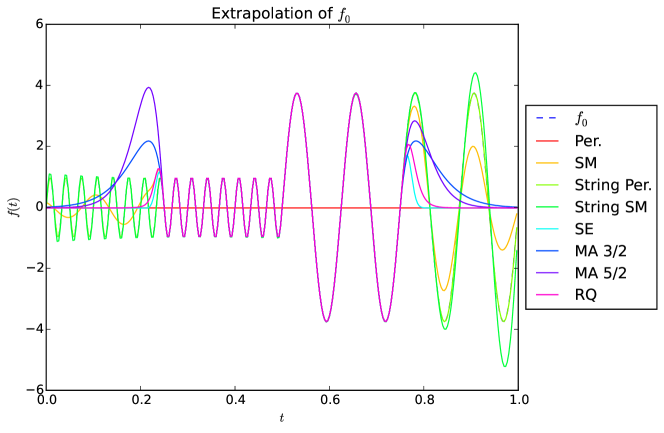
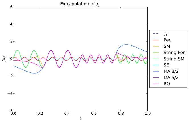
Refer to caption

Refer to caption

Figure 5: Extrapolation of two functions f0subscript𝑓0f_{0} and f1subscript𝑓1f_{1} through Bayesian nonparametric regression under string GP priors and vanilla GP priors with popular and expressive kernels. Each model is trained on [0.25,0.5]0.250.5[0.25,0.5] and extrapolates to [0,1.0]01.0[0,1.0].
Absolute Error Squared Error
Kernel f0subscript𝑓0f_{0} f1subscript𝑓1f_{1} f0subscript𝑓0f_{0} f1subscript𝑓1f_{1}
Squared exponential 1.44±2.40plus-or-minus1.442.401.44\pm 2.40 0.48±0.58plus-or-minus0.480.580.48\pm 0.58 3.50±9.20plus-or-minus3.509.203.50\pm 9.20 0.31±0.64plus-or-minus0.310.640.31\pm 0.64
Rational quadratic 1.39±2.31plus-or-minus1.392.311.39\pm 2.31 0.51±0.83plus-or-minus0.510.830.51\pm 0.83 3.28±8.79plus-or-minus3.288.793.28\pm 8.79 0.43±1.15plus-or-minus0.431.150.43\pm 1.15
Matérn 3/2 1.63±2.53plus-or-minus1.632.531.63\pm 2.53 1.26±1.37plus-or-minus1.261.371.26\pm 1.37 4.26±11.07plus-or-minus4.2611.074.26\pm 11.07 2.06±3.55plus-or-minus2.063.552.06\pm 3.55
Matérn 5/2 1.75±2.77plus-or-minus1.752.771.75\pm 2.77 0.48±0.58plus-or-minus0.480.580.48\pm 0.58 5.00±12.18plus-or-minus5.0012.185.00\pm 12.18 0.31±0.64plus-or-minus0.310.640.31\pm 0.64
Periodic 1.51±2.45plus-or-minus1.512.451.51\pm 2.45 0.53±0.60plus-or-minus0.530.600.53\pm 0.60 3.79±9.62plus-or-minus3.799.623.79\pm 9.62 0.37±0.72plus-or-minus0.370.720.37\pm 0.72
Spec. Mix. (5 comp.) 0.75±1.15plus-or-minus0.751.150.75\pm 1.15 0.39±0.57plus-or-minus0.390.570.39\pm 0.57 0.94±2.46plus-or-minus0.942.460.94\pm 2.46 0.24±0.58plus-or-minus0.240.580.24\pm 0.58
String Spec. Mix. (2 strings, 1 comp.) 0.23±0.84plus-or-minus0.230.840.23\pm 0.84 0.01±0.03plus-or-minus0.010.030.01\pm 0.03 0.21±1.07plus-or-minus0.211.070.21\pm 1.07 0.00±0.00plus-or-minus0.000.00\bf{0.00}\pm\bf{0.00}
String Periodic 0.02±0.02plus-or-minus0.020.02\bf{0.02}\pm\bf{0.02} 0.00±0.01plus-or-minus0.000.01\bf{0.00}\pm\bf{0.01} 0.00±0.00plus-or-minus0.000.00\bf{0.00}\pm\bf{0.00} 0.00±0.00plus-or-minus0.000.00\bf{0.00}\pm\bf{0.00}
Table 2: Predictive accuracies in the extrapolation of the two functions f0subscript𝑓0f_{0} and f1subscript𝑓1f_{1} of Section 6.1 through Bayesian nonparametric regression under string GP priors and vanilla GP priors with popular and expressive kernels. Each model is trained on [0.25,0.5]0.250.5[0.25,0.5] and extrapolates to [0,1.0]01.0[0,1.0]. The predictive errors are reported as average ±plus-or-minus\pm 2 standard deviations.

Refer to caption Refer to caption

Refer to caption Refer to caption

Refer to caption Refer to caption

Refer to caption Refer to caption

Figure 6: Extrapolation of a synthetic function f2subscript𝑓2f_{2} (top left corner), cropped in the middle for training (top right corner), using string GP regression and vanilla GP regression with various popular and expressive kernels.

Refer to caption Refer to caption

Refer to caption Refer to caption

Refer to caption Refer to caption

Refer to caption Refer to caption

Figure 7: Extrapolation of a synthetic function f3subscript𝑓3f_{3} (top left corner), cropped in the middle for training (top right corner), using string GP regression and vanilla GP regression with various popular and expressive kernels.

6.2 Small Scale Heteroskedastic Regression

In our second experiment, we consider illustrating the advantage of the string GP paradigm over the standard GP paradigm, but also over the alternatives of Kim et al. (2005), Gramacy and Lee (2008), Tresp (2000) and Deisenroth and Ng (2015) that consist of considering independent GP experts on disjoint parts of the domain or handling disjoint subsets of the data. Using the motorcycle data set of Silverman (1985), commonly used for the local patterns and heteroskedasticity it exhibits, we show that our approach outperforms the aforementioned competing alternatives, thereby providing empirical evidence that the collaboration between consecutive GP experts introduced in the string GP paradigm vastly improves predictive accuracy and certainty in regression problems with local patterns. We also illustrate learning of the derivative of the latent function, solely from noisy measurements of the latent function.

The observations consist of accelerometer readings taken through time in an experiment on the efficacy of crash helmets. It can be seen at a glance in Figure 8 that the data set exhibits roughly 444 regimes. Firstly, between 00ms and 151515ms the acceleration was negligible. Secondly, the impact slowed down the helmet, resulting in a sharp deceleration between 151515ms and 282828ms. Thirdly, the helmet seems to have bounced back between 282828ms and 323232ms, before it finally gradually slowed down and came to a stop between 323232ms and 606060ms. It can also be noted that the measurement noise seems to have been higher in the second half of the experiment.

We ran 505050 independent random experiments, leaving out 555 points selected uniformly at random from the data set for prediction, the rest being used for training. The models we considered include the vanilla GP regression model, the string GP regression model with marginal maximum likelihood inference as described in Section 5.1, mixtures of independent GP experts acting on disjoint subsets of the data both for training and testing, the Bayesian committee machine (Tresp (2000)), and the robust Bayesian committee machine (Deisenroth and Ng (2015)). We considered string GPs with 444 and 666 strings whose boundary times are learned as part of the maximum likelihood inference. For consistency, we used the resulting partitions of the domain to define the independent experts in the competing alternatives we considered. The Matérn 3/2 kernel was used throughout. The results are reported in Table 3. To gauge the ability of each model to capture the physics of the helmets crash experiment, we have also trained all models with all data points. The results are illustrated in Figures 8 and 9.

It can be seen at a glance from Figure 9 that mixtures of independent GP experts are inappropriate for this experiment as i) the resulting posterior means exhibit discontinuities (for instance at t=30ms𝑡30mst=30\text{ms} and t=40ms𝑡40mst=40\text{ms}) that are inconsistent with the physics of the underlying phenomenon, and ii) they overfit the data towards the end. The foregoing discontinuities do not come as a surprise as each GP regression expert acts on a specific subset of the domain that is disjoint from the ones used by the other experts, both for training and prediction. Thus, there is no guarantee of consistency between expert predictions at the boundaries of the domain partition. Another perspective to this observation is found in noting that postulating independent GP experts, each acting on an element of a partition of the domain, is equivalent to putting as prior on the whole function a stochastic process that is discontinuous at the boundaries of the partition. Thus, the posterior stochastic process should not be expected to be continuous at the boundaries of the domain either.

This discontinuity issue is addressed by the Bayesian committee machine (BCM) and the robust Bayesian committee machine (rBCM) because, despite each independent expert being trained on a disjoint subset of the data, each expert is tasked with making predictions about all test inputs, not just the ones that fall into its input subspace. Each GP expert prediction is therefore continuous on the whole input domain,131313So long as the functional prior is continuous, which is the case here. and the linear weighting schemes operated by the BCM and the rBCM on expert predictions to construct the overall predictive mean preserve continuity. However, we found that the BCM and the rBCM suffer from three pitfalls. First, we found them to be less accurate than any other alternative out-of-sample on this data set (see Table 3). Second, their predictions of latent function values are overly uncertain. This might be due to the fact that, each GP expert being trained only with training samples that lie on its input subspace, its predictions about test inputs that lie farther away from its input subspace will typically be much more uncertain, so that, despite the weighting scheme of the Bayesian committee machine putting more mass on ‘confident’ experts, overall the posterior variance over latent function values might still be much higher than in the standard GP paradigm for instance. This is well illustrated by both the last column of Table 3 and the BCM and rBCM plots in Figure 9. On the contrary, no string GP model suffers from this excess uncertainty problem. Third, the posterior means of the BCM, the rBCM and the vanilla GP regression exhibit oscillations towards the end (t>40ms𝑡40mst>40\text{ms}) that are inconsistent with the experimental setup; the increases in acceleration as the helmet slows down suggested by these posterior means would require an additional source of energy after the bounce.

In addition to being more accurate and more certain about predictions than vanilla GP regression, the BCM and the rBCM (see Table 3), string GP regressions yield posterior mean acceleration profiles that are more consistent with the physics of the experiment: steady speed prior to the shock, followed by a deceleration resulting from the shock, a brief acceleration resulting from the change in direction after the bounce, and finally a smooth slow down due to the dissipation of kinetic energy. Moreover, unlike the vanilla GP regression, the rBCM and the BCM, string GP regressions yield smaller posterior variances towards the beginning and the end of the experiment than in the middle, which is consistent with the fact that the operator would be less uncertain about the acceleration at the beginning and at the end of the experiment—one would indeed expect the acceleration to be null at the beginning and at the end of the experiment. This desirable property can be attributed to the heteroskedasticity of the noise structure in the string GP regression model.

We also learned the derivative of the latent acceleration with respect to time, purely from noisy acceleration measurements using the joint law of a string GP and its derivative (Theorem 2). This is illustrated in Figure 8.

Training Prediction
Log. lik. Log. lik. Absolute Error Squared Error Pred. Std
String GP (4 strings) 388.36±0.36plus-or-minus388.360.36-388.36\pm 0.36 22.16±0.41plus-or-minus22.160.41-22.16\pm 0.41 15.70±1.05plus-or-minus15.701.05\bf{15.70\pm 1.05} 466.47±50.74plus-or-minus466.4750.74\bf{466.47\pm 50.74} 0.70/2.25/3.390.702.253.390.70/2.25/3.39
String GP (6 strings) 367.21±0.43plus-or-minus367.210.43\bf{-367.21\pm 0.43} 21.99±0.37plus-or-minus21.990.37-21.99\pm 0.37 15.89±1.06plus-or-minus15.891.0615.89\pm 1.06 475.59±51.95plus-or-minus475.5951.95475.59\pm 51.95 0.64/2.21/3.460.642.213.46\bf{0.64/2.21/3.46}
Vanilla GP 420.69±0.24plus-or-minus420.690.24-420.69\pm 0.24 22.77±0.24plus-or-minus22.770.24-22.77\pm 0.24 16.84±1.09plus-or-minus16.841.0916.84\pm 1.09 524.18±58.33plus-or-minus524.1858.33524.18\pm 58.33 2.66/3.09/4.942.663.094.942.66/3.09/4.94
Mix. of 4 GPs 388.37±0.38plus-or-minus388.370.38-388.37\pm 0.38 20.90±0.38plus-or-minus20.900.38-20.90\pm 0.38 16.61±1.10plus-or-minus16.611.1016.61\pm 1.10 512.30±56.08plus-or-minus512.3056.08512.30\pm 56.08 1.67/2.85/4.591.672.854.591.67/2.85/4.59
Mix. of 6 GPs 369.05±0.45plus-or-minus369.050.45-369.05\pm 0.45 20.11±0.45plus-or-minus20.110.45\bf{-20.11\pm 0.45} 16.05±1.11plus-or-minus16.051.1116.05\pm 1.11 500.43±58.26plus-or-minus500.4358.26500.43\pm 58.26 0.62/2.83/4.630.622.834.630.62/2.83/4.63
BCM with 4 GPs 419.08±0.30plus-or-minus419.080.30-419.08\pm 0.30 22.94±0.26plus-or-minus22.940.26-22.94\pm 0.26 17.17±1.13plus-or-minus17.171.1317.17\pm 1.13 538.94±61.91plus-or-minus538.9461.91538.94\pm 61.91 7.20/9.92/22.927.209.9222.927.20/9.92/22.92
BCM with 6 GPs 422.15±0.30plus-or-minus422.150.30-422.15\pm 0.30 22.91±0.26plus-or-minus22.910.26-22.91\pm 0.26 16.93±1.12plus-or-minus16.931.1216.93\pm 1.12 533.21±61.78plus-or-minus533.2161.78533.21\pm 61.78 7.09/9.93/25.107.099.9325.107.09/9.93/25.10
rBCM with 4 GPs 419.08±0.30plus-or-minus419.080.30-419.08\pm 0.30 22.99±0.27plus-or-minus22.990.27-22.99\pm 0.27 17.29±1.11plus-or-minus17.291.1117.29\pm 1.11 546.95±61.21plus-or-minus546.9561.21546.95\pm 61.21 5.86/9.08/27.525.869.0827.525.86/9.08/27.52
rBCM with 6 GPs 422.15±0.30plus-or-minus422.150.30-422.15\pm 0.30 22.96±0.28plus-or-minus22.960.28-22.96\pm 0.28 16.79±1.12plus-or-minus16.791.1216.79\pm 1.12 542.95±61.95plus-or-minus542.9561.95542.95\pm 61.95 5.15/8.61/29.155.158.6129.155.15/8.61/29.15
Table 3: Performance comparison between string GPs, vanilla GPs, mixture of independent GPs, the Bayesian committee machine (Tresp (2000)) and the robust Bayesian committee machine (Deisenroth and Ng (2015)) on the motorcycle data set of Silverman (1985). The Matérn 3/2 kernel was used throughout. The domain partitions were learned in the string GP experiments by maximum likelihood. The learned partitions were then reused to allocate data between GP experts in other models. 505050 random runs were performed, each run leaving 555 data points out for testing and using the rest for training. All results (except for predictive standard deviations) are reported as average over the 505050 runs ±plus-or-minus\pm standard error. The last column contains the minimum, average and maximum of the predictive standard deviation of the values of the latent (noise-free) function at all test points across random runs.

Refer to caption

Refer to caption

Figure 8: Posterior mean ±plus-or-minus\pm 2 predictive standard deviations on the motorcycle data set (see Silverman, 1985), under a Matérn 3/2 derivative string GP prior with 6 learned strings. The top figure shows the noisy accelerations measurements and the learned latent function. The bottom function illustrates the derivative of the acceleration with respect to time learned from noisy acceleration samples. Posterior credible bands are over the latent functions rather than noisy measurements, and as such they do not include the measurement noise.

Refer to captionRefer to captionRefer to caption

Refer to captionRefer to captionRefer to caption

Refer to captionRefer to captionRefer to caption

Figure 9: Bayesian nonparametric regressions on the motorcycle data set of Silverman (1985). Models compared are string GP regression, vanilla GP regression, mixture of independent GP regression experts on a partition of the domain, the Bayesian committee machine (BCM) and the robust Bayesian committee machine (rBCM). Domain partitions were learned during string GP maximum likelihood inference (red vertical bars), and reused in other experiments. Blue stars are noisy samples, red lines are posterior means of the latent function and grey bands correspond to ±plus-or-minus\pm 2 predictive standard deviations of the (noise-free) latent function about its posterior mean.

6.3 Large Scale Regression

To illustrate how our approach fares against competing alternatives on a standard large scale problem, we consider predicting arrival delays of commercial flights in the USA in 2008 as studied by Hensman et al. (2013). We choose the same covariates as in Hensman et al. (2013), namely the age of the aircraft (number of years since deployment), distance that needs to be covered, airtime, departure time, arrival time, day of the week, day of the month and month. Unlike Hensman et al. (2013) who only considered commercial flights between January 2008 and April 2008, we consider commercial throughout the whole year, for a total of 5.935.935.93 million records. In addition to the whole data set, we also consider subsets so as to empirically illustrate the sensitivity of computational time to the number of samples. Selected subsets consist of 10,0001000010,000, 100,000100000100,000 and 1,000,00010000001,000,000 records selected uniformly at random. For each data set, we use 2/3232/3 of the records selected uniformly at random for training and we use the remaining 1/3131/3 for testing. In order to level the playing field between stationary and nonstationary approaches, we normalize training and testing data sets.141414More precisely, we substract from every feature sample (both in-sample and out-of-sample) the in-sample mean of the feature and we divide the result by the in-sample standard deviation of the feature. As competing alternatives to string GPs we consider the SVIGP of Hensman et al. (2013), the Bayesian committee machines (BCM) of Tresp (2000), and the robust Bayesian committee machines (rBCM) of Deisenroth and Ng (2015).

As previously discussed the prediction scheme operated by the BCM is Kolmogorov-inconsistent in that the resulting predictive distributions are not consistent by marginalization.151515For instance the predictive distribution of the value of the latent function at a test input x1subscript𝑥1x_{1}, namely f(x1)𝑓subscript𝑥1f(x_{1}), obtained by using {x1}subscript𝑥1\{x_{1}\} as set of test inputs in the BCM, differs from the predictive distribution obtained by using {x1,x2}subscript𝑥1subscript𝑥2\{x_{1},x_{2}\} as set of test inputs in the BCM and then marginalising with respect to the second input x2subscript𝑥2x_{2}. Moreover, jointly predicting all function values by using the set of all test inputs as query set, as originally suggested in Tresp (2000), would be impractical in this experiment given that the BCM requires inverting a covariance matrix of the size of the query set which, considering the numbers of test inputs in this experiment (which we recall can be as high as 1.971.971.97 million), would be computationally intractable. To circumvent this problem we use the BCM algorithm to query one test input at a time. This approach is in-line with that adopted by Deisenroth and Ng (2015), where the authors did not address determining joint predictive distributions over multiple latent function values. For the BCM and rBCM, the number of experts is chosen so that each expert processes 200200200 training points. For SVIGP we use the implementation made available by the The GPy authors (2012–2016), and we use the same configuration as in Hensman et al. (2013). As for string GPs, we use the symmetric sum as link function, and we run two types of experiments, one allowing for inference of change-points (String GP), and the other enforcing a single kernel configuration per input dimension (String GP*). The parameters 𝜶𝜶\bm{\alpha} and 𝜷𝜷\bm{\beta} are chosen so that the prior mean number of change-points in each input dimension is 555% of the number of distinct training and testing values in that input dimension, and so that the prior variance of the foregoing number of change-points is 505050 times the prior mean—the aim is to be uninformative about the number of change-points. We run 10,0001000010,000 iterations of our RJ-MCMC sampler and discarded the first 5,00050005,000 as ‘burn-in’. After burn-in we record the states of the Markov chains for analysis using a 1-in-100 thinning rate. Predictive accuracies are reported in Table 4 and CPU time requirements161616We define CPU time as the cumulative CPU clock resource usage of the whole experiment (training and testing), across child processes and threads, and across CPU cores. are illustrated in Figure 10. We stress that all experiments were run on a multi-core machine, and that we prefer using the cumulative CPU clock resource as time complexity metric, instead of wall-clock time, so as to be agnostic to the number of CPU cores used in the experiments. This metric has the merit of illustrating how the number of CPU cores required grows as a function of the number of training samples for a fixed/desired wall-clock execution time, but also how the wall-clock execution time grows as a function of the number of training samples for a given number of available CPU cores.

The BCM and the rBCM perform the worst in this experiment both in terms of predictive accuracy (Table 4) and total CPU time (Figure 10). The poor scalability of the BCM and the rBCM is primarily due to the testing phase. Indeed, if we denote M𝑀M the total number of experts, then M=N300𝑀𝑁300M=\lceil\frac{N}{300}\rceil, as each expert processes 200200200 training points, of which there are 23N23𝑁\frac{2}{3}N. In the prediction phase, each expert is required to make predictions about all 13N13𝑁\frac{1}{3}N test inputs, which requires evaluating M𝑀M products of an 13N×20013𝑁200\frac{1}{3}N\times 200 matrix with a 200×200200200200\times 200 matrix, which results in a total CPU time requirement that grows in 𝒪(M13N2002)𝒪𝑀13𝑁superscript2002\mathcal{O}(M\frac{1}{3}N200^{2}), which is the same as 𝒪(N2)𝒪superscript𝑁2\mathcal{O}(N^{2}). Given that training CPU time grows linearly in N𝑁N the cumulative training and testing CPU time grows quadratically in N𝑁N. This is well illustrated in Figure 10, where it can be seen that the slopes of total CPU time profiles of the BCM and the rBCM in log-log scale are approximately 222. The airline delays data set was also considered by Deisenroth and Ng (2015), but the authors restricted themselves to a fixed size of the test set of 100,000100000100,000 points. However, this limitation might be restrictive as in many ‘smoothing’ applications, the test data set can be as large as the training data set—neither the BCM nor the rBCM would be sufficiently scalable in such applications.

As for SVIGP, although it was slightly more accurate than string GPs on this data set, it can be noted from Figure 10 that string GPs required 101010 times less CPU resources. In fact we were unable to run the experiment on the full data set with SVIGP—we gave up after 500 CPU hours, or more than a couple of weeks wall-clock time given that the GPy implementation of SVIGP makes little use of multiple cores. As a comparison, the full experiment took 91.091.091.0 hours total CPU time (15absent15\approx 15 hours wall-clock time on our 888 cores machine) when change-points were inferred and 83.1183.1183.11 hours total CPU time (14absent14\approx 14 hours wall-clock time on our 888 cores machine) when change-points were not inferred. Another advantage of additively separable string GPs over GPs, and subsequently over SVIGP, is that they are more interpretable. Indeed, one can determine at a glance from the learned posterior mean string GPs of Figure 11 the effect of each of the 888 covariates considered on arrival delays. It turns out that the three most informative factors in predicting arrival delays are departure time, distance and arrival time, while the age of the aircraft, the day of the week and the day of the month seem to have little to no effect. Finally, posterior distributions of the number of change-points are illustrated in Figure 12, and posterior distributions of the locations of change-points are illustrated in Figure 13.

N String GP String GP* BCM rBCM SVIGP
10,0001000010,000 1.03±0.10plus-or-minus1.030.101.03\pm 0.10 1.06±0.10plus-or-minus1.060.101.06\pm 0.10 1.06±0.10plus-or-minus1.060.101.06\pm 0.10 1.06±0.10plus-or-minus1.060.101.06\pm 0.10 0.90±0.09plus-or-minus0.900.09\bm{0.90\pm 0.09}
100,000100000100,000 0.93±0.03plus-or-minus0.930.030.93\pm 0.03 0.96±0.03plus-or-minus0.960.030.96\pm 0.03 1.66±0.03plus-or-minus1.660.031.66\pm 0.03 1.04±0.04plus-or-minus1.040.041.04\pm 0.04 0.88±0.03plus-or-minus0.880.03\bm{0.88\pm 0.03}
1,000,00010000001,000,000 0.93±0.01plus-or-minus0.930.010.93\pm 0.01 0.92±0.01plus-or-minus0.920.010.92\pm 0.01 N/A N/A 0.82±0.01plus-or-minus0.820.01\bm{0.82\pm 0.01}
5,929,41359294135,929,413 0.90±0.01plus-or-minus0.900.010.90\pm 0.01 0.93±0.01plus-or-minus0.930.010.93\pm 0.01 N/A N/A N/A
Table 4: Predictive mean squared errors (MSEs) ±plus-or-minus\pm one standard error on the airline arrival delays experiment. Squared errors are expressed as fraction of the sample variance of airline arrival delays, and hence are unitless. With this normalisation, a MSE of 1.001.001.00 is as good as using the training mean arrival delays as predictor. The * in String GP* indicates that inference was performed without allowing for change-points. N/A entries correspond to experiments that were not over after 500500500 CPU hours.

Refer to caption

Figure 10: Total CPU time (training and testing) taken by various regression approaches on the airline delays data set as a function of the size of the subset considered, in log-log scale. The experimental setup is described in Section 6.3. The CPU time reflects actual CPU clock resource usage in each experiment, and is therefore agnostic to the number of CPU cores used. It can be regarded as the wall-clock time the experiment would have taken to complete on a single-core computer (with the same CPU frequency). Dashed lines are extrapolated values, and correspond to experiments that did not complete after 500500500 hours of CPU time.

Refer to captionRefer to caption

Refer to captionRefer to caption

Refer to captionRefer to caption

Refer to captionRefer to caption

Figure 11: Posterior mean ±plus-or-minus\pm one posterior standard deviation of univariate string GPs in the airline delays experiment of Section 6.3. Change-points were automatically inferred in this experiment.

Refer to captionRefer to caption

Refer to captionRefer to caption

Refer to captionRefer to caption

Refer to captionRefer to caption

Figure 12: Posterior distributions of the numbers of change-points in each input dimension in the airline delays experiment of Section 6.3.

Refer to captionRefer to caption

Refer to captionRefer to caption

Refer to captionRefer to caption

Figure 13: Posterior distributions of the locations of change-points in each input dimension in the airline delays experiment of Section 6.3. Dimensions that were learned to exhibit no change-point have been omitted here.

6.4 Large Scale Dynamic Asset Allocation

An important feature of our proposed RJ-MCMC sampler (Algorithm 2) is that, unlike the BCM, the rBCM and SVIGP, which are restricted to Bayesian nonparametric regression and classification, Algorithm 2 is agnostic with regard to the likelihood model, so long as it takes the form p(𝒟|𝐟,𝐮)𝑝conditional𝒟𝐟𝐮p(\mathcal{D}|\mathbf{f},\mathbf{u}). Thus, it may be used as is on a wide variety of problems that go beyond classification and regression. In this experiment we aim to illustrate the efficacy of our approach on one such large scale problem in quantitative finance.

6.4.1 Background

Let (xi(t))t>0subscriptsubscript𝑥𝑖𝑡𝑡0\left(x_{i}(t)\right)_{t>0} for i=1,,n𝑖1𝑛i=1,\dots,n be n𝑛n stock price processes. Let (Xi(t))t>0subscriptsubscript𝑋𝑖𝑡𝑡0\left(X_{i}(t)\right)_{t>0} for i=1,,n𝑖1𝑛i=1,\dots,n denote the market capitalisation processes, that is Xi(t)=ni(t)xi(t)subscript𝑋𝑖𝑡subscript𝑛𝑖𝑡subscript𝑥𝑖𝑡X_{i}(t)=n_{i}(t)x_{i}(t) where ni(t)subscript𝑛𝑖𝑡n_{i}(t) is the number of shares in company i𝑖i trading in the market at time t𝑡t. We call long-only portfolio any vector-valued stochastic process π=(π1,,πn)𝜋subscript𝜋1subscript𝜋𝑛\pi=(\pi_{1},\dots,\pi_{n}) taking value on the unit simplex on nsuperscript𝑛\mathbb{R}^{n}, that is

i,t,πi(t)0 and i=1nπi(t)=1.for-all𝑖𝑡subscript𝜋𝑖𝑡0 and superscriptsubscript𝑖1𝑛subscript𝜋𝑖𝑡1\forall i,t,~{}\pi_{i}(t)\geq 0~{}~{}\text{ and }~{}~{}\sum_{i=1}^{n}\pi_{i}(t)=1.

Each process πisubscript𝜋𝑖\pi_{i} represents the proportion of an investor’s wealth invested in (holding) shares in asset i𝑖i. An example long-only portfolio is the market portfolio μ=(μ1,,μn)𝜇subscript𝜇1subscript𝜇𝑛\mu=(\mu_{1},\dots,\mu_{n}) where

μi(t)=Xi(t)X1(t)++Xn(t)subscript𝜇𝑖𝑡subscript𝑋𝑖𝑡subscript𝑋1𝑡subscript𝑋𝑛𝑡\mu_{i}(t)=\frac{X_{i}(t)}{X_{1}(t)+\dots+X_{n}(t)} (47)

is the market weight of company i𝑖i at time t𝑡t, that is its size relative to the total market size (or that of the universe of stocks considered). The market portfolio is very important to practitioners as it is often perceived not be to subject to idiosyncracies, but only to systemic risk. It is often used as an indicator of how the stock market (or a specific universe of stocks) performs as a whole. We denote Zπsubscript𝑍𝜋Z_{\pi} the value process of a portfolio π𝜋\pi with initial capital Zπ(0)subscript𝑍𝜋0Z_{\pi}(0). That is, Zπ(t)subscript𝑍𝜋𝑡Z_{\pi}(t) is the wealth at time t𝑡t of an investor who had an initial wealth of Zπ(0)subscript𝑍𝜋0Z_{\pi}(0), and dynamically re-allocated all his wealth between the n𝑛n stocks in our universe up to time t𝑡t following the continuous-time strategy π𝜋\pi.

A mathematical theory has recently emerged, namely stochastic portfolio theory (SPT) (see Karatzas and Fernholz, 2009) that studies the stochastic properties of the wealth processes of certain portfolios called functionally-generated portfolio under realistic assumptions on the market capitalisation processes (Xi(t))t>0subscriptsubscript𝑋𝑖𝑡𝑡0\left(X_{i}(t)\right)_{t>0}. Functionally-generated portfolios are rather specific in that the allocation at time t𝑡t, namely (π1(t),,πn(t))subscript𝜋1𝑡subscript𝜋𝑛𝑡(\pi_{1}(t),\dots,\pi_{n}(t)), solely depends on the market weights vector (μ1(t),,μn(t))subscript𝜇1𝑡subscript𝜇𝑛𝑡(\mu_{1}(t),\dots,\mu_{n}(t)). Nonetheless, some functionally-generated portfolios πsuperscript𝜋\pi^{*} have been found that, under the mild (so-called diversity) condition

μmax,0<μmax<1s.t.in,tT,μi(t)μmax,formulae-sequencesubscript𝜇max0subscript𝜇max1s.t.for-all𝑖𝑛formulae-sequence𝑡𝑇subscript𝜇𝑖𝑡subscript𝜇max\exists\mu_{\text{max}},0<\mu_{\text{max}}<1~{}~{}~{}\text{s.t.}~{}~{}~{}\forall i\leq n,~{}t\leq T,~{}~{}~{}\mu_{i}(t)\leq\mu_{\text{max}}, (48)

outperform the market portfolio over the time horizon [0,T]0𝑇[0,T] with probability one (see Vervuurt and Karatzas, 2015; Karatzas and Fernholz, 2009). More precisely,

(Zπ(T)Zμ(T))=1and(Zπ(T)>Zμ(T))>0.subscript𝑍superscript𝜋𝑇subscript𝑍𝜇𝑇1andsubscript𝑍superscript𝜋𝑇subscript𝑍𝜇𝑇0\mathbb{P}\left(Z_{\pi^{*}}(T)\geq Z_{\mu}(T)\right)=1~{}~{}~{}\text{and}~{}~{}~{}\mathbb{P}\left(Z_{\pi^{*}}(T)>Z_{\mu}(T)\right)>0. (49)

Galvanized by this result, we here consider the inverse problem consisting of learning from historical market data a portfolio whose wealth process has desirable user-specified properties. This inverse problem is perhaps more akin to the problems faced by investment professionals: i) their benchmarks depend on the investment vehicles pitched to investors and may vary from one vehicle to another, ii) they have to take into account liquidity costs, and iii) they often find it more valuable to go beyond market weights and leverage multiple company characteristics in their investment strategies.

6.4.2 Model Construction

We consider portfolios πf=(π1f,,πnf)superscript𝜋𝑓superscriptsubscript𝜋1𝑓superscriptsubscript𝜋𝑛𝑓\pi^{f}=\left(\pi_{1}^{f},\dots,\pi_{n}^{f}\right) of the form

πif(t)=f(ci(t))f(c1(t))++f(cn(t)),superscriptsubscript𝜋𝑖𝑓𝑡𝑓subscript𝑐𝑖𝑡𝑓subscript𝑐1𝑡𝑓subscript𝑐𝑛𝑡\pi_{i}^{f}(t)=\frac{f(c_{i}(t))}{f(c_{1}(t))+\dots+f(c_{n}(t))}, (50)

where ci(t)dsubscript𝑐𝑖𝑡superscript𝑑c_{i}(t)\in\mathbb{R}^{d} are some quantifiable characteristics of asset i𝑖i that may be observed in the market at time t𝑡t, and f𝑓f is a positive-valued function. Portfolios of this form include all functionally-generated portfolios studied in SPT as a special case.171717We refer the reader to Karatzas and Fernholz (2009) for the definition of functionally-generated portfolios. A crucial departure of our approach from the aforementioned type of portfolios is that the market characteristics processes cisubscript𝑐𝑖c_{i} need not be restricted to size-based information, and may contain additional information such as social media sentiments, stock price path-properties, but also characteristics relative to other stocks such as performance relative to the best/worst performing stock last week/month/year etc. We place a mean-zero string GP prior on logf𝑓\log f. Given some historical data 𝒟𝒟\mathcal{D} corresponding to a training time horizon [0,T]0𝑇[0,T], the likelihood model p(𝒟|πf)𝑝conditional𝒟superscript𝜋𝑓p\left(\mathcal{D}|\pi^{f}\right) is defined by the investment professional and reflects the extent to which applying the investment strategy πfsuperscript𝜋𝑓\pi^{f} over the training time horizon would have achieved a specific investment objective. An example investment objective is to achieve a high excess return relative to a benchmark portfolio α𝛼\alpha

𝒰ER(πf)=logZπf(T)logZα(T).subscript𝒰ERsuperscript𝜋𝑓subscript𝑍superscript𝜋𝑓𝑇subscript𝑍𝛼𝑇\mathcal{U}_{\text{ER}}\left(\pi^{f}\right)=\log Z_{\pi^{f}}(T)-\log Z_{\alpha}(T). (51)

α𝛼\alpha can be the market portfolio (as in SPT) or any stock index. Other risk-adjusted investment objectives may also be used. One such objective is to achieve a high Sharpe-ratio, defined as

𝒰SR(πf)=r¯2521Tt=1T(r(t)r¯)2,subscript𝒰SRsuperscript𝜋𝑓¯𝑟2521𝑇superscriptsubscript𝑡1𝑇superscript𝑟𝑡¯𝑟2\mathcal{U}_{\text{SR}}\left(\pi^{f}\right)=\frac{\bar{r}\sqrt{252}}{\sqrt{\frac{1}{T}\sum_{t=1}^{T}(r(t)-\bar{r})^{2}}}, (52)

where the time t𝑡t is in days, r(t):=logZπf(t)logZπf(t1)assign𝑟𝑡subscript𝑍superscript𝜋𝑓𝑡subscript𝑍superscript𝜋𝑓𝑡1r(t):=\log Z_{\pi^{f}}(t)-\log Z_{\pi^{f}}(t-1) are the daily returns the portfolio πfsuperscript𝜋𝑓\pi^{f} and r¯=1Tt=1Tr(t)¯𝑟1𝑇superscriptsubscript𝑡1𝑇𝑟𝑡\bar{r}=\frac{1}{T}\sum_{t=1}^{T}r(t) its average daily return. More generally, denoting 𝒰(πf)𝒰superscript𝜋𝑓\mathcal{U}\left(\pi^{f}\right) the performance of the portfolio πfsuperscript𝜋𝑓\pi^{f} over the training horizon [0,T]0𝑇[0,T] (as per the user-defined investment objective), we may choose as likelihood model a distribution over 𝒰(πf)𝒰superscript𝜋𝑓\mathcal{U}\left(\pi^{f}\right) that reflects what the investment professional considers good and bad performance. For instance, in the case of the excess return relative to a benchmark portfolio or the Sharpe ratio, we may choose 𝒰(πf)𝒰superscript𝜋𝑓\mathcal{U}\left(\pi^{f}\right) to be supported on ]0,+[]0,+\infty[ (for instance 𝒰(πf)𝒰superscript𝜋𝑓\mathcal{U}\left(\pi^{f}\right) can be chosen to be Gamma distributed) so as to express that portfolios that do not outperform the benchmark or loose money overall in the training data are not of interest. We may then choose the mean and standard deviation of the Gamma distribution based on our expectation as to what performance a good candidate portfolio can achieve, and how confident we feel about this expectation. Overall we have,

p(𝒟|πf)=γ(𝒰(πf);αe,βe),𝑝conditional𝒟superscript𝜋𝑓𝛾𝒰superscript𝜋𝑓subscript𝛼𝑒subscript𝛽𝑒p\left(\mathcal{D}|\pi^{f}\right)=\gamma\left(\mathcal{U}\left(\pi^{f}\right);\alpha_{e},\beta_{e}\right), (53)

where γ(.;α,β)\gamma(.;\alpha,\beta) is the probability density function of the Gamma distribution. Noting, from Equation (50) that πf(t)superscript𝜋𝑓𝑡\pi^{f}(t) only depends on f𝑓f through its values at (c1(t),,cn(t))subscript𝑐1𝑡subscript𝑐𝑛𝑡(c_{1}(t),\dots,c_{n}(t)), and assuming that 𝒰(πf)𝒰superscript𝜋𝑓\mathcal{U}\left(\pi^{f}\right) only depends on πfsuperscript𝜋𝑓\pi^{f} evaluated at a finite number of times (as it is the case for excess returns and the Sharpe ratio), it follows that 𝒰(πf)𝒰superscript𝜋𝑓\mathcal{U}(\pi^{f}) only depends on 𝐟𝐟\mathbf{f}, a vector of values of f𝑓f at a finite number of points. Hence the likelihood model, which we may rewrite as

p(𝒟|𝐟)=γ(𝒰(πif);αe,βe),𝑝conditional𝒟𝐟𝛾𝒰superscriptsubscript𝜋𝑖𝑓subscript𝛼𝑒subscript𝛽𝑒p(\mathcal{D}|\mathbf{f})=\gamma\left(\mathcal{U}\left(\pi_{i}^{f}\right);\alpha_{e},\beta_{e}\right), (54)

is of the form required by the RJ-MCMC sampler previously developed. By sampling from the posterior distribution p(𝐟,𝐟,𝐟,𝐟|𝒟)𝑝𝐟superscript𝐟𝐟conditionalsuperscript𝐟𝒟p(\mathbf{f},\mathbf{f}^{*},\nabla\mathbf{f},\nabla\mathbf{f}^{*}|\mathcal{D}), the hope is to learn a portfolio that did well during the training horizon, to analyse the sensitivity of its investment strategy to the underlying market characteristics through the gradient of f𝑓f, and to evaluate the learned investment policy on future market conditions.

6.4.3 Experimental Setup

The universe of stocks we considered for this experiment are the constituents of the S&P 500 index, accounting for changes in constituents over time and corporate events. We used the period 1st January 1990 to 31st December 2004 for training and we tested the learned portfolio during the period 1st January 2005 to 31st December 2014. We rebalanced the portfolio daily, for a total of 2.522.522.52 million input points at which the latent function f𝑓f must be learned. We considered as market characteristics the market weight (CAP), the latest return on asset (ROA) defined as the ratio between the net yearly income and the total assets as per the latest balance sheet of the company known at the time of investment, the previous close-to-close return (PR), the close-to-close return before the previous (PR2), and the S&P long and short term credit rating (LCR and SCR). While the market weight is a company size characteristic, the ROA reflects how well a company performs relative to its size, and we hope that S&P credit ratings will help further discriminate successful companies from others. The close-to-close returns are used to learn possible ‘momentum’ patterns from the data. The data originate from the CRSP and Compustat databases. In the experiments we considered as performance metric the annualised excess return 𝒰ER-EWPsubscript𝒰ER-EWP\mathcal{U}_{\text{ER-EWP}} relative to the equally-weighted portfolio. We found the equally-weighted portfolio to be a harder benchmark to outperform than the market portfolio. We chose αesubscript𝛼𝑒\alpha_{e} and βesubscript𝛽𝑒\beta_{e} in Equation (54) so that the mean of the Gamma distribution is 10.010.010.0 and its variance 0.50.50.5, which expresses a very greedy investment target.

It is worth pointing out that none of the scalable GP alternatives previously considered can cope with our likelihood model Equation (54). We compared the performance of the learned string GP portfolio out-of-sample to those of the best three SPT portfolios studied in Vervuurt and Karatzas (2015), namely the equally weighted portfolio

πiEWP(t)=1n,superscriptsubscript𝜋𝑖EWP𝑡1𝑛\pi_{i}^{\text{EWP}}(t)=\frac{1}{n}, (55)

and the diversity weighted portfolios

πiDWP(t;p)=μi(t)pμ1(t)p++μn(t)p,superscriptsubscript𝜋𝑖DWP𝑡𝑝subscript𝜇𝑖superscript𝑡𝑝subscript𝜇1superscript𝑡𝑝subscript𝜇𝑛superscript𝑡𝑝\pi_{i}^{\text{DWP}}(t;p)=\frac{\mu_{i}(t)^{p}}{\mu_{1}(t)^{p}+\dots+\mu_{n}(t)^{p}}, (56)

with parameter p𝑝p equals to 0.50.5-0.5 and 0.50.50.5, and the market portfolio. Results are provided Table 5, and Figure 14 displays the evolution of the wealth process of each strategy. It can be seen that the learned string GP strategy considerably outperforms the next best SPT portfolio. This experiment not only demonstrates (once more) that string GPs scale to large scale problems, it also illustrates that our inference scheme is able to unlock commercial value in new intricate large scale applications where no alternative is readily available. In effect, this application was first introduced by Kom Samo and Vervuurt (2016), where the authors used a Gaussian process prior on a Cartesian grid and under a separable covariance function so as to speed up inference with Kronecker techniques. Although the resulting inference scheme has time complexity that is linear in the total number of points on the grid, for a given grid resolution, the time complexity grows exponentially in the dimension of the input space (that is the number of trading characteristics), which is impractical for d4𝑑4d\geq 4. On the other hand, string GPs allow for a time complexity that grows linearly with the number of trading characteristics, thereby enabling the learning of subtler market inefficiencies from the data.
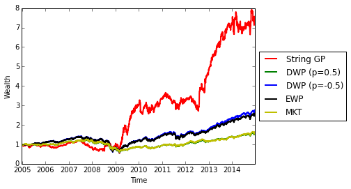
Refer to caption

Figure 14: Evolution of the wealth processes of various long-only trading strategies on the S&P 500500500 universe of stocks between 1st January 2005 (where we assume a starting wealth of 111) and 31st December 2014. The String GP strategy was learned using market data from 1st January 1990 to 31st December 2004 as descried in Section 6.4. EWP refers to the equally-weighted portfolio, MKT refers to the market portfolio (which weights stocks proportionally to their market capitalisations) and DWP (p) refers to the diversity-weighted portfolio with exponent p𝑝p (which weights stocks proportionally to the p𝑝p-th power of their market weights).
Strategy Sharpe Ratio Zπ(T)/ZEWP(T)subscript𝑍𝜋𝑇subscript𝑍EWP𝑇Z_{\pi}(T)/Z_{\text{EWP}}(T) Avg. Ann. Ret.
String GP 0.730.73\bm{0.73} 2.872.87\bm{2.87} 22.0722.07\bm{22.07}%
DWP (p=0.5𝑝0.5p=-0.5) 0.550.550.55 1.071.071.07 10.5610.5610.56%
EWP 0.530.530.53 1.001.001.00 9.849.849.84%
MKT 0.340.340.34 0.620.620.62 4.774.774.77%
DWP (p=0.5𝑝0.5p=0.5) 0.330.330.33 0.610.610.61 4.514.514.51%
Table 5: Performance of various long-only trading strategies on the S&P 500500500 universe of stocks between 1st January 2005 (where we assume a starting wealth of 111) and 31st December 2014. The String GP strategy was learned using market data from 1st January 1990 to 31st December 2004 as descried in Section 6.4. EWP refers to the equally-weighted portfolio, MKT refers to the market portfolio (which weights stocks proportionally to their market capitalisations) and DWP (p) refers to the diversity-weighted portfolio with exponent p𝑝p (which weights stocks proportionally to the p𝑝p-th power of the market weight of the asset). Zπ(T)subscript𝑍𝜋𝑇Z_{\pi}(T) denotes the terminal wealth of strategy π𝜋\pi, and Avg. Ann. Ret. is the strategy’s equivalent constant annual return over the test horizon.

7 Discussion

In this paper, we introduce a novel class of smooth functional priors (or stochastic processes), which we refer to as string GPs, with the aim of simultaneously addressing the lack of scalability and the lack of flexibility of Bayesian kernel methods. Unlike existing approaches, such as Gaussian process priors (Rasmussen and Williams (2006)) or student-t process priors (Shah et al. (2014)), which are parametrised by global mean and covariance functions, and which postulate fully dependent finite-dimensional marginals, the alternative construction we propose adopts a local perspective and the resulting finite-dimensional marginals exhibit conditional independence structures. Our local approach to constructing string GPs provides a principled way of postulating that the latent function we wish to learn might exhibit locally homogeneous patterns, while the conditional independence structures constitute the core ingredient needed for developing scalable inference methods. Moreover, we provide theoretical results relating our approach to Gaussian processes, and we illustrate that our approach can often be regarded as a more scalable and/or more flexible extension. We argue and empirically illustrate that string GPs present an unparalleled opportunity for learning local patterns in small scale regression problems using nothing but standard Gaussian process regression techniques. More importantly, we propose a novel scalable RJ-MCMC inference scheme to learn latent functions in a wide variety of machine learning tasks, while simultaneously determining whether the data set exhibits local patterns, how many types of local patterns the data might exhibit, and where do changes in these patterns are likely to occur. The proposed scheme has time complexity and memory requirement that are both linear in the sample size N𝑁N. When the number of available computing cores is at least equal to the dimension d𝑑d of the input space, the time complexity is independent from the dimension of the input space. Else, the time complexity grows in 𝒪(dN)𝒪𝑑𝑁\mathcal{O}(dN). The memory requirement grows in 𝒪(dN)𝒪𝑑𝑁\mathcal{O}(dN). We empirically illustrate that our approach scales considerably better than competing alternatives on a standard benchmark data set, and is able to process data sizes that competing approaches cannot handle in a reasonable time.

7.1 Limitations

The main limitation of our approach is that, unlike the standard GP paradigm in which the time complexity of marginal likelihood evaluation does not depend on the dimension of the input space (other than through the evaluation of the Gram matrix), the string GP paradigm requires a number of computing cores that increases linearly with the dimension of the input space, or alternatively has a time complexity linear in the input space dimension on single-core machines. This is a by-product of the fact that in the string GP paradigm, we jointly infer the latent function and its gradient. If the gradient of the latent function is inferred in the standard GP paradigm, the resulting complexity will also be linear in the input dimension. That being said, overall our RJ-MCMC inference scheme will typically scale better per iteration to large input dimensions than gradient-based marginal likelihood inference in the standard GP paradigm, as the latter typically requires numerically evaluating an Hessian matrix, which requires computing the marginal likelihood a number of times per iterative update that grows quadratically with the input dimension. In contrast, a Gibbs cycle in our MCMC sampler has worst case time complexity that is linear in the input dimension.

7.2 Extensions

Some of the assumptions we have made in the construction of string GPs and membrane GPs can be relaxed, which we consider in detail below.

7.2.1 Stronger Global Regularity

We could have imposed more (multiple continuous differentiability) or less (continuity) regularity as boundary conditions in the construction of string GPs. We chose continuous differentiability as it is a relatively mild condition guaranteed by most popular kernels, and yet the corresponding treatment can be easily generalised to other regularity requirements. It is also possible to allow for discontinuity at a boundary time aksubscript𝑎𝑘a_{k} by replacing μkbsuperscriptsubscript𝜇𝑘𝑏\mu_{k}^{b} and ΣkbsuperscriptsubscriptΣ𝑘𝑏\Sigma_{k}^{b} in Equation (5) with Makksubscriptsubscript𝑀subscript𝑎𝑘𝑘{}_{k}M_{a_{k}} and Kak;akksubscriptsubscriptKsubscript𝑎𝑘subscript𝑎𝑘𝑘{}_{k}\textbf{K}_{a_{k};a_{k}} respectively, or equivalently by preventing any communication between the k𝑘k-th and the (k+1)𝑘1(k+1)-th strings. This would effectively be equivalent to having two independent string GPs on [a0,ak]subscript𝑎0subscript𝑎𝑘[a_{0},a_{k}] and ]ak,aK]]a_{k},a_{K}].

7.2.2 Differential Operators as Link Functions

Our framework can be further extended to allow differential operators as link functions, thereby considering the latent multivariate function to infer as the response of a differential system to independent univariate string GP excitations. The RJ-MCMC sampler we propose in Section 5 would still work in this framework, with the only exception that, when the differential operator is of first order, the latent multivariate function will be continuous but not differentiable, except if global regularity is upgraded as discussed above. Moreover, Proposition 5 can be generalised to first order linear differential operators.

7.2.3 Distributed String GPs

The RJ-MCMC inference scheme we propose may be easily adapted to handle applications where the data set is so big that it has to be stored across multiple clusters, and inference techniques have to be developed as data flow graphs181818A data flow graph is a computational (directed) graph whose nodes represent calculations (possibly taking place on different computing units) and directed edges correspond to data flowing between calculations or computing units. (for instance using libraries such as TensorFlow).

To do so, the choice of string boundary times can be adapted so that each string has the same number of inner input coordinates, and such that in total there are as many strings across dimensions as a target number of available computing cores. We may then place a prior on kernel memberships similar to that of previous sections. Here, the change-points may be restricted to coincide with boundary times, and we may choose priors such that the sets of change-points are independent between input dimensions. In each input dimension the prior on the number of change-points can be chosen to be a truncated Poisson distribution (truncated to never exceed the total number of boundary times), and conditional on their number we may choose change-points to be uniformly distributed in the set of boundary times. In so doing, any two strings whose shared boundary time is not a change-point will be driven by the same kernel configuration.

This new setup presents no additional theoretical or practical challenges, and the RJ-MCMC techniques previously developed are easily adaptable to jointly learn change-points and function values. Unlike the case we developed in previous sections where an update of the univariate string GP corresponding to an input dimension, say the j𝑗j-th, requires looping through all distinct j𝑗j-th input coordinates, here no step in the inference scheme requires a full view of the data set in any input dimension. Full RJ-MCMC inference can be constructed as a data flow graph. An example such graph is constructed as follows. The leaves correspond to computing cores responsible for generating change-points and kernel configurations, and mapping strings to kernel configurations. The following layer is made of compute cores that use kernel configurations coming out of the previous layer to sequentially compute boundary conditions corresponding to a specific input dimension—there are d𝑑d such compute cores, where d𝑑d is the input dimension. These compute cores then pass computed boundary conditions to subsequent compute cores we refer to as string compute cores. Each string compute core is tasked with computing derivative string GP values for a specific input dimension and for a specific string in that input dimension, conditional on previously computed boundary conditions. These values are then passed to a fourth layer of compute cores, each of which being tasked with computing function and gradient values corresponding to a small subset of training inputs from previously computed derivative string GP values. The final layers then computes the log-likelihood using a distributed algorithm such as Map-Reduce when possible. This proposal data flow graph is illustrated Figure 15.

We note that the approaches of Kim et al. (2005), Gramacy and Lee (2008), Tresp (2000), and Deisenroth and Ng (2015) also allow for fully-distributed inference on regression problems. Distributed string GP RJ-MCMC inference improves on these in that it places little restriction on the type of likelihood. Moreover, unlike Kim et al. (2005) and Gramacy and Lee (2008) that yield discontinuous latent functions, string GPs are continuously differentiable, and unlike Tresp (2000) and Deisenroth and Ng (2015), local experts in the string GP paradigm (i.e. strings) are driven by possibly different sets of hyper-parameters, which facilitates the learning of local patterns.

7.2.4 Approximate MCMC for I.I.D. Observations Likelihoods

As discussed in Section 5.2, the bottleneck of our proposed inference scheme is the evaluation of likelihood. When the likelihood factorises across training samples, the linear time complexity of our proposed approach can be further reduced using a Monte Carlo approximation of the log-likelihood (see for instance Bardenet et al. (2014) and references therein). Although the resulting Markov chain will typically not converge to the true posterior distribution, in practice its stationary distribution can be sufficiently close to the true posterior when reasonable Monte Carlo sample sizes are used. Convergence results of such approximations have recently been studied by Bardenet et al. (2014) and Alquier et al. (2016). We expect this extension to speed-up inference when the number of compute cores is in the order of magnitude of the input dimension, but we would recommend the previously mentioned fully-distributed string GP inference extension when compute cores are not scarce.

7.2.5 Variational Inference

It would be useful to develop suitable variational methods for inference under string GP priors, that we hope will scale similarly to our proposed RJ-MCMC sampler but will converge faster. We anticipate that the main challenge here will perhaps be the learning of model complexity, that is the number of distinct kernel configurations in each input dimension.

Change-points computations Computation of boundary conditions Computation of inner String GP values conditional on boundary conditions Computation of latent function values and gradients Computation of partial log-likelihoods (i.e. Map) Sum of partial log-likelihoods (i.e. Reduce) Boundary Conditions String GP Values and Derivatives Latent Function and Gradient Values Kernel Hyper-Parameters Partial Log-Likelihoods
Figure 15: Example data flow graph for fully-distributed string GP inference under an i.i.d observations likelihood model. Here the input space is three-dimensional to ease illustration. Filled circles represent compute cores, and edges correspond to flows of data. Compute cores with the same colour (green, red or yellow) perform operations pertaining to the same input dimension, while black-filled circles represent compute cores performing cross-dimensional operations. The blue rectangle plays the role of a hub that relays string GP values to the compute cores that need them to compute the subset of latent function values and gradients they are responsible for. These values are then used to compute the log-likelihood in a distributed fashion using the Map-Reduce algorithm. Each calculation in the corresponding RJ-MCMC sampler would be initiated at one of the compute cores, and would trigger updates of all edges accessible from that compute core.

Acknowledgments

Yves-Laurent is a Google Fellow in Machine Learning and would like to acknowledge support from the Oxford-Man Institute. Wharton Research Data Services (WRDS) was used in preparing the data for Section 6.4 of this paper. This service and the data available thereon constitute valuable intellectual property and trade secrets of WRDS and/or its third-party suppliers.

Appendix Appendix A

We begin by recalling Kolmogorov’s extension theorem, which we will use to prove the existence of derivative Gaussian processes and string Gaussian processes.

Theorem 7

(Kolmogorov’s extension theorem, (Øksendal, 2003, Theorem 2.1.5))
Let I𝐼I be an interval, let all t1,,tiI,i,nformulae-sequencesubscript𝑡1subscript𝑡𝑖𝐼𝑖𝑛superscriptt_{1},\dots,t_{i}\in I,~{}i,n\in\mathbb{N}^{*}, let νt1,,tisubscript𝜈subscript𝑡1subscript𝑡𝑖\nu_{t_{1},\dots,t_{i}} be probability measures on nisuperscript𝑛𝑖\mathbb{R}^{ni} such that:

νtπ(1),,tπ(i)(Fπ(1),,Fπ(i))=νt1,,ti(F1,,Fi)subscript𝜈subscript𝑡𝜋1subscript𝑡𝜋𝑖subscript𝐹𝜋1subscript𝐹𝜋𝑖subscript𝜈subscript𝑡1subscript𝑡𝑖subscript𝐹1subscript𝐹𝑖\nu_{t_{\pi(1)},\dots,t_{\pi(i)}}(F_{\pi(1)},\dots,F_{\pi(i)})=\nu_{t_{1},\dots,t_{i}}(F_{1},\dots,F_{i}) (57)

for all permutations π𝜋\pi on {1,,i}1𝑖\{1,\dots,i\} and

νt1,,ti(F1,,Fi)=νt1,,ti,ti+1,,ti+m(F1,,Fi,n,,n)subscript𝜈subscript𝑡1subscript𝑡𝑖subscript𝐹1subscript𝐹𝑖subscript𝜈subscript𝑡1subscript𝑡𝑖subscript𝑡𝑖1subscript𝑡𝑖𝑚subscript𝐹1subscript𝐹𝑖superscript𝑛superscript𝑛\displaystyle\nu_{t_{1},\dots,t_{i}}(F_{1},\dots,F_{i})=\nu_{t_{1},\dots,t_{i},t_{i+1},\dots,t_{i+m}}(F_{1},\dots,F_{i},\mathbb{R}^{n},\dots,\mathbb{R}^{n}) (58)

for all m𝑚superscriptm\in\mathbb{N}^{*} where the set on the right hand side has a total of i+m𝑖𝑚i+m factors. Then there exists a probability space (Ω,,)Ω(\Omega,\mathcal{F},\mathbb{P}) and an nsuperscript𝑛\mathbb{R}^{n} valued stochastic process (Xt)tIsubscriptsubscript𝑋𝑡𝑡𝐼(X_{t})_{t\in I} on ΩΩ\Omega,

Xt:Ωn:subscript𝑋𝑡Ωsuperscript𝑛X_{t}:\Omega\to\mathbb{R}^{n}

such that

νt1,,ti(F1,,Fi)=(Xt1F1,,XtiFi)subscript𝜈subscript𝑡1subscript𝑡𝑖subscript𝐹1subscript𝐹𝑖formulae-sequencesubscript𝑋subscript𝑡1subscript𝐹1subscript𝑋subscript𝑡𝑖subscript𝐹𝑖\nu_{t_{1},\dots,t_{i}}(F_{1},\dots,F_{i})=\mathbb{P}(X_{t_{1}}\in F_{1},\dots,X_{t_{i}}\in F_{i}) (59)

for all t1,,tiI,iformulae-sequencesubscript𝑡1subscript𝑡𝑖𝐼𝑖superscriptt_{1},\dots,t_{i}\in I,~{}i\in\mathbb{N}^{*} and for all Borel sets F1,,Fisubscript𝐹1subscript𝐹𝑖F_{1},\dots,F_{i}.

It is easy to see that every stochastic process satisfies the permutation and marginalisation conditions (57) and (58). The power of Kolmogorov’s extension theorem is that it states that those two conditions are sufficient to guarantee the existence of a stochastic process.

Appendix Appendix B Proof of Proposition 1

In this section we prove Proposition 1, which we recall below.

Proposition 1 (Derivative Gaussian processes)
Let I𝐼I be an interval, k:I×I:𝑘𝐼𝐼k:I\times I\rightarrow\mathbb{R} a 𝒞2superscript𝒞2\mathcal{C}^{2} symmetric positive semi-definite function,191919𝒞1superscript𝒞1\mathcal{C}^{1} (resp. 𝒞2superscript𝒞2\mathcal{C}^{2}) functions denote functions that are once (resp. twice) continuously differentiable on their domains. m:I:𝑚𝐼m:I\rightarrow\mathbb{R} a 𝒞1superscript𝒞1\mathcal{C}^{1} function.

(A) There exists a 2superscript2\mathbb{R}^{2}-valued stochastic process (Dt)tI,Dt=(zt,zt)subscriptsubscript𝐷𝑡𝑡𝐼subscript𝐷𝑡subscript𝑧𝑡superscriptsubscript𝑧𝑡\left(D_{t}\right)_{t\in I},~{}D_{t}=(z_{t},z_{t}^{\prime}), such that for all t1,,tnIsubscript𝑡1subscript𝑡𝑛𝐼t_{1},\dots,t_{n}\in I,

(zt1,,ztn,zt1,,ztn)subscript𝑧subscript𝑡1subscript𝑧subscript𝑡𝑛superscriptsubscript𝑧subscript𝑡1superscriptsubscript𝑧subscript𝑡𝑛(z_{t_{1}},\dots,z_{t_{n}},z_{t_{1}}^{\prime},\dots,z_{t_{n}}^{\prime})

is a Gaussian vector with mean

(m(t1),,m(tn),dmdt(t1),,dmdt(tn))𝑚subscript𝑡1𝑚subscript𝑡𝑛d𝑚dtsubscript𝑡1d𝑚dtsubscript𝑡𝑛\left(m(t_{1}),\dots,m(t_{n}),\frac{\text{d}m}{\text{dt}}(t_{1}),\dots,\frac{\text{d}m}{\text{dt}}(t_{n})\right)

and covariance matrix such that

cov(zti,ztj)=k(ti,tj),cov(zti,ztj)=ky(ti,tj),andcov(zti,ztj)=2kxy(ti,tj).formulae-sequencecovsubscript𝑧subscript𝑡𝑖subscript𝑧subscript𝑡𝑗𝑘subscript𝑡𝑖subscript𝑡𝑗formulae-sequencecovsubscript𝑧subscript𝑡𝑖superscriptsubscript𝑧subscript𝑡𝑗𝑘𝑦subscript𝑡𝑖subscript𝑡𝑗andcovsuperscriptsubscript𝑧subscript𝑡𝑖superscriptsubscript𝑧subscript𝑡𝑗superscript2𝑘𝑥𝑦subscript𝑡𝑖subscript𝑡𝑗\text{cov}(z_{t_{i}},z_{t_{j}})=k(t_{i},t_{j}),~{}~{}~{}\text{cov}(z_{t_{i}},z_{t_{j}}^{\prime})=\frac{\partial k}{\partial y}(t_{i},t_{j}),~{}~{}~{}\text{and}~{}~{}~{}\text{cov}(z_{t_{i}}^{\prime},z_{t_{j}}^{\prime})=\frac{\partial^{2}k}{\partial x\partial y}(t_{i},t_{j}).

We herein refer to (Dt)tIsubscriptsubscript𝐷𝑡𝑡𝐼(D_{t})_{t\in I} as a derivative Gaussian process.

(B) (zt)tIsubscriptsubscript𝑧𝑡𝑡𝐼(z_{t})_{t\in I} is a Gaussian process with mean function m𝑚m, covariance function k𝑘k and that is 𝒞1superscript𝒞1\mathcal{C}^{1} in the L2superscript𝐿2L^{2} (mean square) sense.

(C) (zt)tIsubscriptsubscriptsuperscript𝑧𝑡𝑡𝐼(z^{\prime}_{t})_{t\in I} is a Gaussian process with mean function dmdtd𝑚dt\frac{\text{d}m}{\text{dt}} and covariance function 2kxysuperscript2𝑘𝑥𝑦\frac{\partial^{2}k}{\partial x\partial y}. Moreover, (zt)tIsubscriptsubscriptsuperscript𝑧𝑡𝑡𝐼(z^{\prime}_{t})_{t\in I} is the L2superscript𝐿2L^{2} derivative of the process (zt)tIsubscriptsubscript𝑧𝑡𝑡𝐼(z_{t})_{t\in I}.

Proof 

Appendix B.1 Proof of Proposition 1 (A)

Firstly, we need to show that the matrix suggested in the proposition as the covariance matrix of (zt1,,ztn,zt1,,ztn)subscript𝑧subscript𝑡1subscript𝑧subscript𝑡𝑛superscriptsubscript𝑧subscript𝑡1superscriptsubscript𝑧subscript𝑡𝑛(z_{t_{1}},\dots,z_{t_{n}},z_{t_{1}}^{\prime},\dots,z_{t_{n}}^{\prime}) is indeed positive semi-definite. To do so, we will show that it is the limit of positive definite matrices (which is sufficient to conclude it is positive semi-definite, as xTMnx0superscript𝑥𝑇subscript𝑀𝑛𝑥0x^{T}M_{n}x\geq 0 for a convergent sequence of positive definite matrices implies xTMx0superscript𝑥𝑇subscript𝑀𝑥0x^{T}M_{\infty}x\geq 0).

Let k𝑘k be as in the proposition, hh such that in,ti+hIformulae-sequencefor-all𝑖𝑛subscript𝑡𝑖𝐼\forall i\leq n,~{}t_{i}+h\in I and (z~t)tIsubscriptsubscript~𝑧𝑡𝑡𝐼(\tilde{z}_{t})_{t\in I} be a Gaussian process with covariance function k𝑘k. The vector

(z~t1,,z~tn,z~t1+hz~t1h,,z~tn+hz~tnh)subscript~𝑧subscript𝑡1subscript~𝑧subscript𝑡𝑛subscript~𝑧subscript𝑡1subscript~𝑧subscript𝑡1subscript~𝑧subscript𝑡𝑛subscript~𝑧subscript𝑡𝑛\left(\tilde{z}_{t_{1}},\dots,\tilde{z}_{t_{n}},\frac{\tilde{z}_{t_{1}+h}-\tilde{z}_{t_{1}}}{h},\dots,\frac{\tilde{z}_{t_{n}+h}-\tilde{z}_{t_{n}}}{h}\right)

is a Gaussian vector whose covariance matrix is positive definite and such that

cov(z~ti,z~tj)=k(ti,tj),covsubscript~𝑧subscript𝑡𝑖subscript~𝑧subscript𝑡𝑗𝑘subscript𝑡𝑖subscript𝑡𝑗\displaystyle\text{cov}\left(\tilde{z}_{t_{i}},\tilde{z}_{t_{j}}\right)=k(t_{i},t_{j}), (60)
cov(z~ti,z~tj+hz~tjh)=k(ti,tj+h)k(ti,tj)h,covsubscript~𝑧subscript𝑡𝑖subscript~𝑧subscript𝑡𝑗subscript~𝑧subscript𝑡𝑗𝑘subscript𝑡𝑖subscript𝑡𝑗𝑘subscript𝑡𝑖subscript𝑡𝑗\displaystyle\text{cov}\left(\tilde{z}_{t_{i}},\frac{\tilde{z}_{t_{j}+h}-\tilde{z}_{t_{j}}}{h}\right)=\frac{k(t_{i},t_{j}+h)-k(t_{i},t_{j})}{h}, (61)

and

cov(z~ti+hz~tih,z~tj+hz~tjh)covsubscript~𝑧subscript𝑡𝑖subscript~𝑧subscript𝑡𝑖subscript~𝑧subscript𝑡𝑗subscript~𝑧subscript𝑡𝑗\displaystyle\text{cov}\left(\frac{\tilde{z}_{t_{i}+h}-\tilde{z}_{t_{i}}}{h},\frac{\tilde{z}_{t_{j}+h}-\tilde{z}_{t_{j}}}{h}\right)
=1h2(k(ti+h,tj+h)k(ti+h,tj)k(ti,tj+h)+k(ti,tj)).absent1superscript2𝑘subscript𝑡𝑖subscript𝑡𝑗𝑘subscript𝑡𝑖subscript𝑡𝑗𝑘subscript𝑡𝑖subscript𝑡𝑗𝑘subscript𝑡𝑖subscript𝑡𝑗\displaystyle=\frac{1}{h^{2}}\left(k(t_{i}+h,t_{j}+h)-k(t_{i}+h,t_{j})-k(t_{i},t_{j}+h)+k(t_{i},t_{j})\right). (62)

As k𝑘k is 𝒞2superscript𝒞2\mathcal{C}^{2}, hk(x,y+h)𝑘𝑥𝑦h\to k(x,y+h) admits a second order Taylor expansion about h=00h=0 for every x𝑥x, and we have:

k(x,y+h)𝑘𝑥𝑦\displaystyle k(x,y+h) =k(x,y)+ky(x,y)h+122ky2(x,y)h2+o(h2)=k(y+h,x).absent𝑘𝑥𝑦𝑘𝑦𝑥𝑦12superscript2𝑘superscript𝑦2𝑥𝑦superscript2𝑜superscript2𝑘𝑦𝑥\displaystyle=k(x,y)+\frac{\partial k}{\partial y}(x,y)h+\frac{1}{2}\frac{\partial^{2}k}{\partial y^{2}}(x,y)h^{2}+o(h^{2})=k(y+h,x). (63)

Similarly, hk(x+h,y+h)𝑘𝑥𝑦h\to k(x+h,y+h) admits a second order Taylor expansion about h=00h=0 for every x,y𝑥𝑦x,~{}y and we have:

k(x+h,y+h)=𝑘𝑥𝑦absent\displaystyle k(x+h,y+h)= k(x,y)+[kx(x,y)+ky(x,y)]h+[2kxy(x,y)+122kx2(x,y)\displaystyle~{}k(x,y)+\left[\frac{\partial k}{\partial x}(x,y)+\frac{\partial k}{\partial y}(x,y)\right]h+\Bigg{[}\frac{\partial^{2}k}{\partial x\partial y}(x,y)+\frac{1}{2}\frac{\partial^{2}k}{\partial x^{2}}(x,y)
+122ky2(x,y)]h2+o(h2).\displaystyle+\frac{1}{2}\frac{\partial^{2}k}{\partial y^{2}}(x,y)\Bigg{]}h^{2}+o(h^{2}). (64)

Hence,

k(ti,tj+h)k(ti,tj)=ky(ti,tj)h+o(h),𝑘subscript𝑡𝑖subscript𝑡𝑗𝑘subscript𝑡𝑖subscript𝑡𝑗𝑘𝑦subscript𝑡𝑖subscript𝑡𝑗𝑜\displaystyle k(t_{i},t_{j}+h)-k(t_{i},t_{j})=\frac{\partial k}{\partial y}(t_{i},t_{j})h+o(h), (65)

and

k(ti+h,tj+h)k(ti+h,tj)k(ti,tj+h)+k(ti,tj)=2kxy(ti,tj)h2+o(h2).𝑘subscript𝑡𝑖subscript𝑡𝑗𝑘subscript𝑡𝑖subscript𝑡𝑗𝑘subscript𝑡𝑖subscript𝑡𝑗𝑘subscript𝑡𝑖subscript𝑡𝑗superscript2𝑘𝑥𝑦subscript𝑡𝑖subscript𝑡𝑗superscript2𝑜superscript2\displaystyle k(t_{i}+h,t_{j}+h)-k(t_{i}+h,t_{j})-k(t_{i},t_{j}+h)+k(t_{i},t_{j})=\frac{\partial^{2}k}{\partial x\partial y}(t_{i},t_{j})h^{2}+o(h^{2}). (66)

Dividing Equation (65) by hh, dividing Equation (66) by h2superscript2h^{2}, and taking the limits, we obtain:

limh0cov(z~ti,z~tj+hz~tjh)=ky(ti,tj),0covsubscript~𝑧subscript𝑡𝑖subscript~𝑧subscript𝑡𝑗subscript~𝑧subscript𝑡𝑗𝑘𝑦subscript𝑡𝑖subscript𝑡𝑗\underset{h\to 0}{\lim}~{}\text{cov}\left(\tilde{z}_{t_{i}},\frac{\tilde{z}_{t_{j}+h}-\tilde{z}_{t_{j}}}{h}\right)=\frac{\partial k}{\partial y}(t_{i},t_{j}),

and

limh0cov(z~ti+hz~tih,z~tj+hz~tjh)=2kxy(ti,tj),subscript0covsubscript~𝑧subscript𝑡𝑖subscript~𝑧subscript𝑡𝑖subscript~𝑧subscript𝑡𝑗subscript~𝑧subscript𝑡𝑗superscript2𝑘𝑥𝑦subscript𝑡𝑖subscript𝑡𝑗\lim_{h\to 0}~{}\text{cov}\left(\frac{\tilde{z}_{t_{i}+h}-\tilde{z}_{t_{i}}}{h},\frac{\tilde{z}_{t_{j}+h}-\tilde{z}_{t_{j}}}{h}\right)=\frac{\partial^{2}k}{\partial x\partial y}(t_{i},t_{j}),

which corresponds to the covariance structure of Proposition 1. In other words the proposed covariance structure is indeed positive semi-definite.

Let νt1,,tn𝒩subscriptsuperscript𝜈𝒩subscript𝑡1subscript𝑡𝑛\nu^{\mathcal{N}}_{t_{1},\dots,t_{n}} be the Gaussian probability measure corresponding to the joint distribution of (zt1,,ztn,zt1,,ztn)subscript𝑧subscript𝑡1subscript𝑧subscript𝑡𝑛superscriptsubscript𝑧subscript𝑡1superscriptsubscript𝑧subscript𝑡𝑛(z_{t_{1}},\dots,z_{t_{n}},z_{t_{1}}^{\prime},\dots,z_{t_{n}}^{\prime}) as per the Proposition 1, and let νt1,,tnDsubscriptsuperscript𝜈𝐷subscript𝑡1subscript𝑡𝑛\nu^{D}_{t_{1},\dots,t_{n}} be the measure on the Borel σ𝜎\sigma-algebra (2××2)n times \mathcal{B}(\underbrace{\mathbb{R}^{2}\times\dots\times\mathbb{R}^{2})}_{n\text{ times }} such that for any 2n2𝑛2n intervals I11,I12,,In1,In2subscript𝐼11subscript𝐼12subscript𝐼𝑛1subscript𝐼𝑛2I_{11},I_{12},\dots,I_{n1},I_{n2},

νt1,,tnD(I11×I12,,In1×In2):=νt1,,tn𝒩(I11,,In1,I12,,In2).assignsubscriptsuperscript𝜈𝐷subscript𝑡1subscript𝑡𝑛subscript𝐼11subscript𝐼12subscript𝐼𝑛1subscript𝐼𝑛2subscriptsuperscript𝜈𝒩subscript𝑡1subscript𝑡𝑛subscript𝐼11subscript𝐼𝑛1subscript𝐼12subscript𝐼𝑛2\displaystyle\nu^{D}_{t_{1},\dots,t_{n}}(I_{11}\times I_{12},\dots,I_{n1}\times I_{n2}):=\nu^{\mathcal{N}}_{t_{1},\dots,t_{n}}(I_{11},\dots,I_{n1},I_{12},\dots,I_{n2}). (67)

The measures νt1,,tnDsubscriptsuperscript𝜈𝐷subscript𝑡1subscript𝑡𝑛\nu^{D}_{t_{1},\dots,t_{n}} are the finite dimensional measures corresponding to the stochastic object (Dt)tIsubscriptsubscript𝐷𝑡𝑡𝐼(D_{t})_{t\in I} sampled at times t1,,tnsubscript𝑡1subscript𝑡𝑛t_{1},\dots,t_{n}. They satisfy the time permutation and marginalisation conditions of Kolmogorov’s extension theorem as the Gaussian measures νt1,,tn𝒩subscriptsuperscript𝜈𝒩subscript𝑡1subscript𝑡𝑛\nu^{\mathcal{N}}_{t_{1},\dots,t_{n}} do. Hence, the 2superscript2\mathbb{R}^{2}-valued stochastic process (Dt)tIsubscriptsubscript𝐷𝑡𝑡𝐼(D_{t})_{t\in I} defined in Proposition 1 does exist.

Appendix B.2 Proof of Proposition 1 (B)

That (zt)tIsubscriptsubscript𝑧𝑡𝑡𝐼(z_{t})_{t\in I} is a Gaussian process results from the fact that the marginals (zt1,,ztn)subscript𝑧subscript𝑡1subscript𝑧subscript𝑡𝑛(z_{t_{1}},\dots,z_{t_{n}}) are Gaussian vectors with mean (m(t1),,m(tn))𝑚subscript𝑡1𝑚subscript𝑡𝑛(m(t_{1}),\dots,m(t_{n})) and covariance matrix [k(ti,tj)]i,j[1..n][k(t_{i},t_{j})]_{i,j\in[1..n]}. The fact that (zt)tIsubscriptsubscript𝑧𝑡𝑡𝐼(z_{t})_{t\in I} is 𝒞1superscript𝒞1\mathcal{C}^{1} in the L2superscript𝐿2L^{2} sense is a direct consequence of the twice continuous differentiability of k𝑘k.

Appendix B.3 Proof of Proposition 1 (C)

In effect, it follows from Proposition 1(A) that zt+hzthztsubscript𝑧𝑡subscript𝑧𝑡subscriptsuperscript𝑧𝑡\frac{z_{t+h}-z_{t}}{h}-z^{\prime}_{t} is a Gaussian random variable with mean

m(t+h)m(t)hdmdt(t)𝑚𝑡𝑚𝑡d𝑚dt𝑡\frac{m(t+h)-m(t)}{h}-\frac{\text{d}m}{\text{dt}}(t)

and variance

k(t+h,t+h)2k(t+h,t)+k(t,t)2ky(t+h,t)h+2ky(t,t)h+2kxy(t,t)h2h2.𝑘𝑡𝑡2𝑘𝑡𝑡𝑘𝑡𝑡2𝑘𝑦𝑡𝑡2𝑘𝑦𝑡𝑡superscript2𝑘𝑥𝑦𝑡𝑡superscript2superscript2\frac{k(t+h,t+h)-2k(t+h,t)+k(t,t)-2\frac{\partial k}{\partial y}(t+h,t)h+2\frac{\partial k}{\partial y}(t,t)h+\frac{\partial^{2}k}{\partial x\partial y}(t,t)h^{2}}{h^{2}}.

Taking the second order Taylor expansion of the numerator in the fraction above about h=00h=0 we get o(h2)𝑜superscript2o(h^{2}), hence

limh0Var(zt+hzthzt)=0.0Varsubscript𝑧𝑡subscript𝑧𝑡subscriptsuperscript𝑧𝑡0\underset{h\to 0}{\lim}~{}\text{Var}\left(\frac{z_{t+h}-z_{t}}{h}-z^{\prime}_{t}\right)=0.

We also have

limh0E(zt+hzthzt)=dmdt(t)E(zt)=0.0Esubscript𝑧𝑡subscript𝑧𝑡subscriptsuperscript𝑧𝑡d𝑚𝑑𝑡𝑡Esubscriptsuperscript𝑧𝑡0\underset{h\to 0}{\lim}~{}\text{E}\left(\frac{z_{t+h}-z_{t}}{h}-z^{\prime}_{t}\right)=\frac{\text{d}m}{dt}(t)-\text{E}(z^{\prime}_{t})=0.

Therefore,

limh0E[(zt+hzthzt)2]=0,0Edelimited-[]superscriptsubscript𝑧𝑡subscript𝑧𝑡subscriptsuperscript𝑧𝑡20\underset{h\to 0}{\lim}~{}\text{E}\left[\left(\frac{z_{t+h}-z_{t}}{h}-z^{\prime}_{t}\right)^{2}\right]=0,

which proves that (zt)subscriptsuperscript𝑧𝑡(z^{\prime}_{t}) is the L2superscript𝐿2L^{2} derivative of (zt)subscript𝑧𝑡(z_{t}). The fact that (zt)subscriptsuperscript𝑧𝑡(z^{\prime}_{t}) is a Gaussian process with mean function dmdtd𝑚𝑑𝑡\frac{\text{d}m}{dt} and covariance function 2kxysuperscript2𝑘𝑥𝑦\frac{\partial^{2}k}{\partial x\partial y} is a direct consequence of the distribution of the marginals (zt1,,ztn)superscriptsubscript𝑧subscript𝑡1superscriptsubscript𝑧subscript𝑡𝑛(z_{t_{1}}^{\prime},\dots,z_{t_{n}}^{\prime}). Moreover, the continuity of (zt)subscriptsuperscript𝑧𝑡(z^{\prime}_{t}) in the L2superscript𝐿2L^{2} sense is a direct consequence of the continuity of 2kxysuperscript2𝑘𝑥𝑦\frac{\partial^{2}k}{\partial x\partial y} (see Rasmussen and Williams, 2006, p. 81 4.1.1).  

Appendix Appendix C Proof of Theorem 2

In this section we prove Theorem 2 which we recall below.

Theorem 2 (String Gaussian process)
Let a0<<ak<<aKsubscript𝑎0subscript𝑎𝑘subscript𝑎𝐾a_{0}<\dots<a_{k}<\dots<a_{K}, I=[a0,aK]𝐼subscript𝑎0subscript𝑎𝐾I=[a_{0},a_{K}] and let p𝒩(x;μ,Σ)subscript𝑝𝒩𝑥𝜇Σp_{\mathcal{N}}(x;\mu,\Sigma) be the multivariate Gaussian density with mean vector μ𝜇\mu and covariance matrix ΣΣ\Sigma. Furthermore, let (mk:[ak1,ak])k[1..K](m_{k}:[a_{k-1},a_{k}]\to\mathbb{R})_{k\in[1..K]} be 𝒞1superscript𝒞1\mathcal{C}^{1} functions, and (kk:[ak1,ak]×[ak1,ak])k[1..K](k_{k}:[a_{k-1},a_{k}]\times[a_{k-1},a_{k}]\to\mathbb{R})_{k\in[1..K]} be 𝒞3superscript𝒞3\mathcal{C}^{3} symmetric positive semi-definite functions, neither degenerate at ak1subscript𝑎𝑘1a_{k-1}, nor degenerate at aksubscript𝑎𝑘a_{k} given ak1subscript𝑎𝑘1a_{k-1}.

(A) There exists an 2superscript2\mathbb{R}^{2}-valued stochastic process (SDt)tI,SDt=(zt,zt)subscript𝑆subscript𝐷𝑡𝑡𝐼𝑆subscript𝐷𝑡subscript𝑧𝑡superscriptsubscript𝑧𝑡(SD_{t})_{t\in I},~{}SD_{t}=(z_{t},z_{t}^{\prime}) satisfying the following conditions:

1) The probability density of (SDa0,,SDaK)𝑆subscript𝐷subscript𝑎0𝑆subscript𝐷subscript𝑎𝐾(SD_{a_{0}},\dots,SD_{a_{K}}) reads:

pb(x0,,xK):=k=0Kp𝒩(xk;μkb,Σkb)assignsubscript𝑝𝑏subscript𝑥0subscript𝑥𝐾superscriptsubscriptproduct𝑘0𝐾subscript𝑝𝒩subscript𝑥𝑘subscriptsuperscript𝜇𝑏𝑘superscriptsubscriptΣ𝑘𝑏p_{b}(x_{0},\dots,x_{K}):=\prod_{k=0}^{K}p_{\mathcal{N}}\left(x_{k};\mu^{b}_{k},\Sigma_{k}^{b}\right)
where:Σ0b=Ka0;a01,k>0Σkb=Kak;akkKak;ak1kKak1;ak11kKak;ak1Tk,formulae-sequencewhere:superscriptsubscriptΣ0𝑏subscriptsubscriptKsubscript𝑎0subscript𝑎01for-all𝑘0superscriptsubscriptΣ𝑘𝑏subscriptsubscriptKsubscript𝑎𝑘subscript𝑎𝑘𝑘subscriptsubscriptKsubscript𝑎𝑘subscript𝑎𝑘1𝑘subscriptsuperscriptsubscriptKsubscript𝑎𝑘1subscript𝑎𝑘11𝑘subscriptsuperscriptsubscriptKsubscript𝑎𝑘subscript𝑎𝑘1𝑇𝑘\text{where:}~{}~{}~{}~{}\Sigma_{0}^{b}={}_{1}\textbf{K}_{a_{0};a_{0}},~{}~{}\forall~{}k>0~{}~{}~{}\Sigma_{k}^{b}={}_{k}\textbf{K}_{a_{k};a_{k}}-{}_{k}\textbf{K}_{a_{k};a_{k-1}}~{}{}_{k}\textbf{K}_{a_{k-1};a_{k-1}}^{-1}~{}{}_{k}\textbf{K}_{a_{k};a_{k-1}}^{T},
μ0b=Ma01,k>0μkb=Makk+Kak;ak1kKak1;ak11k(xk1Mak1k),formulae-sequencesuperscriptsubscript𝜇0𝑏subscriptsubscriptMsubscript𝑎01for-all𝑘0subscriptsuperscript𝜇𝑏𝑘subscriptsubscriptMsubscript𝑎𝑘𝑘subscriptsubscriptKsubscript𝑎𝑘subscript𝑎𝑘1𝑘subscriptsuperscriptsubscriptKsubscript𝑎𝑘1subscript𝑎𝑘11𝑘subscript𝑥𝑘1subscriptsubscriptMsubscript𝑎𝑘1𝑘\mu_{0}^{b}={}_{1}\textbf{M}_{a_{0}},~{}~{}\forall~{}k>0~{}~{}~{}\mu^{b}_{k}={}_{k}\textbf{M}_{a_{k}}+{}_{k}\textbf{K}_{a_{k};a_{k-1}}~{}{}_{k}\textbf{K}_{a_{k-1};a_{k-1}}^{-1}(x_{k-1}-{}_{k}\textbf{M}_{a_{k-1}}),
withKu;vk=[kk(u,v)kky(u,v)kkx(u,v)2kkxy(u,v)],andMuk=[mk(u)dmkdt(u)].formulae-sequencewithsubscriptsubscriptK𝑢𝑣𝑘matrixsubscript𝑘𝑘𝑢𝑣subscript𝑘𝑘𝑦𝑢𝑣subscript𝑘𝑘𝑥𝑢𝑣superscript2subscript𝑘𝑘𝑥𝑦𝑢𝑣andsubscriptsubscriptM𝑢𝑘matrixsubscript𝑚𝑘𝑢𝑑subscript𝑚𝑘𝑑𝑡𝑢\text{with}~{}~{}~{}~{}{}_{k}\textbf{K}_{u;v}=\begin{bmatrix}k_{k}(u,v)&\frac{\partial k_{k}}{\partial y}(u,v)\\ \frac{\partial k_{k}}{\partial x}(u,v)&\frac{\partial^{2}k_{k}}{\partial x\partial y}(u,v)\end{bmatrix},~{}~{}~{}~{}\text{and}~{}~{}~{}~{}{}_{k}\textbf{M}_{u}=\begin{bmatrix}m_{k}(u)\\ \frac{dm_{k}}{dt}(u)\end{bmatrix}.

2) Conditional on (SDak=xk)k[0..K](SD_{a_{k}}=x_{k})_{k\in[0..K]}, the restrictions (SDt)t]ak1,ak[,k[1..K](SD_{t})_{t\in]a_{k-1},a_{k}[},~{}k\in[1..K] are independent conditional derivative Gaussian processes, respectively with unconditional mean function mksubscript𝑚𝑘m_{k} and unconditional covariance function kksubscript𝑘𝑘k_{k} and that are conditioned to take values xk1subscript𝑥𝑘1x_{k-1} and xksubscript𝑥𝑘x_{k} at ak1subscript𝑎𝑘1a_{k-1} and aksubscript𝑎𝑘a_{k} respectively. We refer to (SDt)tIsubscript𝑆subscript𝐷𝑡𝑡𝐼(SD_{t})_{t\in I} as a string derivative Gaussian process, and to its first coordinate (zt)tIsubscriptsubscript𝑧𝑡𝑡𝐼(z_{t})_{t\in I} as a string Gaussian process namely,

(zt)tI𝒮𝒢𝒫({ak},{mk},{kk}).similar-tosubscriptsubscript𝑧𝑡𝑡𝐼𝒮𝒢𝒫subscript𝑎𝑘subscript𝑚𝑘subscript𝑘𝑘(z_{t})_{t\in I}\sim\mathcal{SGP}(\{a_{k}\},\{m_{k}\},\{k_{k}\}).

(B) The string Gaussian process (zt)tIsubscriptsubscript𝑧𝑡𝑡𝐼(z_{t})_{t\in I} defined in (A) is 𝒞1superscript𝒞1\mathcal{C}^{1} in the L2superscript𝐿2L^{2} sense and its L2superscript𝐿2L^{2} derivative is the process (zt)tIsubscriptsuperscriptsubscript𝑧𝑡𝑡𝐼(z_{t}^{\prime})_{t\in I} defined in (A).

Proof 

Appendix C.1 Proof of Theorem 2 (A)

We will once again turn to Kolmogorov’s extension theorem to prove the existence of the stochastic process (SDt)tIsubscript𝑆subscript𝐷𝑡𝑡𝐼(SD_{t})_{t\in I}. The core of the proof is in the finite dimensional measures implied by Theorem 2 (A-1) and (A-2). Let {tik]ak1,ak[}i[1..Nk],k[1..K]\left\{t^{k}_{i}\in]a_{k-1},a_{k}[\right\}_{i\in[1..N_{k}],k\in[1..K]} be n𝑛n times. We first formally construct the finite dimensional measures implied by Theorem 2 (A-1) and (A-2), and then verify that they satisfy the conditions of Kolmogorov’s extension theorem.

Let us define the measure νt11,,tN11,,t1K,,tNKK,a0,,aKSDsubscriptsuperscript𝜈𝑆𝐷superscriptsubscript𝑡11superscriptsubscript𝑡subscript𝑁11superscriptsubscript𝑡1𝐾superscriptsubscript𝑡subscript𝑁𝐾𝐾subscript𝑎0subscript𝑎𝐾\nu^{SD}_{t_{1}^{1},\dots,t_{N_{1}}^{1},\dots,t_{1}^{K},\dots,t_{N_{K}}^{K},a_{0},\dots,a_{K}} as the probability measure having density with respect to the Lebesgue measure on (2××2)1+n+K times \mathcal{B}(\underbrace{\mathbb{R}^{2}\times\dots\times\mathbb{R}^{2})}_{1+n+K\text{ times }} that reads:

pSD(xt11,,xtN11,,xt1K,,xtNKK,xa0,,xaK)=subscript𝑝𝑆𝐷subscript𝑥superscriptsubscript𝑡11subscript𝑥superscriptsubscript𝑡subscript𝑁11subscript𝑥superscriptsubscript𝑡1𝐾subscript𝑥superscriptsubscript𝑡subscript𝑁𝐾𝐾subscript𝑥subscript𝑎0subscript𝑥subscript𝑎𝐾absent\displaystyle p_{SD}(x_{t_{1}^{1}},\dots,x_{t_{N_{1}}^{1}},\dots,x_{t_{1}^{K}},\dots,x_{t_{N_{K}}^{K}},x_{a_{0}},\dots,x_{a_{K}})= pb(xa0,,xaK)×\displaystyle p_{b}(x_{a_{0}},\dots,x_{a_{K}})\times
k=1Kp𝒩xak1,xak(xt1k,,xtNkk)superscriptsubscriptproduct𝑘1𝐾subscriptsuperscript𝑝subscript𝑥subscript𝑎𝑘1subscript𝑥subscript𝑎𝑘𝒩subscript𝑥superscriptsubscript𝑡1𝑘subscript𝑥superscriptsubscript𝑡subscript𝑁𝑘𝑘\displaystyle\prod_{k=1}^{K}p^{x_{a_{k-1}},x_{a_{k}}}_{\mathcal{N}}(x_{t_{1}^{k}},\dots,x_{t_{N_{k}}^{k}}) (68)

where pbsubscript𝑝𝑏p_{b} is as per Theorem 2 (A-1) and p𝒩xak1,xak(xt1k,,xtNkk)subscriptsuperscript𝑝subscript𝑥subscript𝑎𝑘1subscript𝑥subscript𝑎𝑘𝒩subscript𝑥superscriptsubscript𝑡1𝑘subscript𝑥superscriptsubscript𝑡subscript𝑁𝑘𝑘p^{x_{a_{k-1}},x_{a_{k}}}_{\mathcal{N}}(x_{t_{1}^{k}},\dots,x_{t_{N_{k}}^{k}}) is the (Gaussian) pdf of the joint distribution of the values at times {tik]ak1,ak[}\{t_{i}^{k}\in]a_{k-1},a_{k}[\} of the conditional derivative Gaussian process with unconditional mean functions mksubscript𝑚𝑘m_{k} and unconditional covariance functions kksubscript𝑘𝑘k_{k} that is conditioned to take values xak1=(zak1,zak1)subscript𝑥subscript𝑎𝑘1subscript𝑧subscript𝑎𝑘1subscriptsuperscript𝑧subscript𝑎𝑘1x_{a_{k-1}}=(z_{a_{k-1}},z^{\prime}_{a_{k-1}}) and xak=(zak,zak)subscript𝑥subscript𝑎𝑘subscript𝑧subscript𝑎𝑘subscriptsuperscript𝑧subscript𝑎𝑘x_{a_{k}}=(z_{a_{k}},z^{\prime}_{a_{k}}) at times ak1subscript𝑎𝑘1a_{k-1} and aksubscript𝑎𝑘a_{k} respectively (the corresponding—conditional—mean and covariance functions are derived from Equations (3 and 4). Let us extend the family of measures νSDsuperscript𝜈𝑆𝐷\nu^{SD} to cases where some or all boundary times aksubscript𝑎𝑘a_{k} are missing, by integrating out the corresponding variables in Equation (Appendix C.1). For instance when a0subscript𝑎0a_{0} and a1subscript𝑎1a_{1} are missing,

νt11,,tN11,,t1K,,tNKK,a2,,aKSD(T11,,TN11,,T1K,,TNKK,A2,,AK)subscriptsuperscript𝜈𝑆𝐷superscriptsubscript𝑡11superscriptsubscript𝑡subscript𝑁11superscriptsubscript𝑡1𝐾superscriptsubscript𝑡subscript𝑁𝐾𝐾subscript𝑎2subscript𝑎𝐾superscriptsubscript𝑇11superscriptsubscript𝑇subscript𝑁11superscriptsubscript𝑇1𝐾superscriptsubscript𝑇subscript𝑁𝐾𝐾subscript𝐴2subscript𝐴𝐾\displaystyle\nu^{SD}_{t_{1}^{1},\dots,t_{N_{1}}^{1},\dots,t_{1}^{K},\dots,t_{N_{K}}^{K},a_{2},\dots,a_{K}}(T_{1}^{1},\dots,T_{N_{1}}^{1},\dots,T_{1}^{K},\dots,T_{N_{K}}^{K},A_{2},\dots,A_{K})
:=νt11,,tN11,,t1K,,tNKK,a0,,aKSD(T11,,TN11,,T1K,,TNKK,2,2,A2,,AK)assignabsentsubscriptsuperscript𝜈𝑆𝐷superscriptsubscript𝑡11superscriptsubscript𝑡subscript𝑁11superscriptsubscript𝑡1𝐾superscriptsubscript𝑡subscript𝑁𝐾𝐾subscript𝑎0subscript𝑎𝐾superscriptsubscript𝑇11superscriptsubscript𝑇subscript𝑁11superscriptsubscript𝑇1𝐾superscriptsubscript𝑇subscript𝑁𝐾𝐾superscript2superscript2subscript𝐴2subscript𝐴𝐾\displaystyle:=\nu^{SD}_{t_{1}^{1},\dots,t_{N_{1}}^{1},\dots,t_{1}^{K},\dots,t_{N_{K}}^{K},a_{0},\dots,a_{K}}(T_{1}^{1},\dots,T_{N_{1}}^{1},\dots,T_{1}^{K},\dots,T_{N_{K}}^{K},\mathbb{R}^{2},\mathbb{R}^{2},A_{2},\dots,A_{K})

where Aisubscript𝐴𝑖A_{i} and Tjisubscriptsuperscript𝑇𝑖𝑗T^{i}_{j} are rectangle in 2superscript2\mathbb{R}^{2}. Finally, we extend the family of measures νSDsuperscript𝜈𝑆𝐷\nu^{SD} to any arbitrary set of indices {t1,,tn}subscript𝑡1subscript𝑡𝑛\{t_{1},\dots,t_{n}\} as follows:

νt1,,tnSD(T1,,Tn):=νtπ(1),,tπ(n)SD(Tπ(1),,Tπ(n)),assignsubscriptsuperscript𝜈𝑆𝐷subscript𝑡1subscript𝑡𝑛subscript𝑇1subscript𝑇𝑛subscriptsuperscript𝜈𝑆𝐷subscript𝑡superscript𝜋1subscript𝑡superscript𝜋𝑛subscript𝑇superscript𝜋1subscript𝑇superscript𝜋𝑛\displaystyle\nu^{SD}_{t_{1},\dots,t_{n}}(T_{1},\dots,T_{n}):=\nu^{SD}_{t_{\pi^{*}(1)},\dots,t_{\pi^{*}(n)}}(T_{\pi^{*}(1)},\dots,T_{\pi^{*}(n)}), (70)

where πsuperscript𝜋\pi^{*} is a permutation of {1,,n}1𝑛\{1,\dots,n\} such that {tπ(1),,tπ(n)}subscript𝑡superscript𝜋1subscript𝑡superscript𝜋𝑛\{t_{\pi^{*}(1)},\dots,t_{\pi^{*}(n)}\} verify the following conditions:

  1. 1.

    i,j,if ti]ak11,ak1[,tj]ak21,ak2[, and k1<k2,\forall~{}i,~{}j,~{}\text{if }t_{i}\in]a_{k_{1}-1},a_{k_{1}}[,~{}t_{j}\in]a_{k_{2}-1},a_{k_{2}}[,\text{ and }k_{1}<k_{2}, then Idx(ti)<Idx(tj).Idxsubscript𝑡𝑖Idxsubscript𝑡𝑗\text{Idx}(t_{i})<\text{Idx}(t_{j}). Where Idx(ti)Idxsubscript𝑡𝑖\text{Idx}(t_{i}) stands for the index of tisubscript𝑡𝑖t_{i} in {tπ(1),,tπ(n)}subscript𝑡superscript𝜋1subscript𝑡superscript𝜋𝑛\{t_{\pi^{*}(1)},\dots,t_{\pi^{*}(n)}\};

  2. 2.

    if ti{a0,,aK} and tj{a0,,aK}subscript𝑡𝑖subscript𝑎0subscript𝑎𝐾 and subscript𝑡𝑗subscript𝑎0subscript𝑎𝐾t_{i}\notin\{a_{0},\dots,a_{K}\}\text{ and }t_{j}\in\{a_{0},\dots,a_{K}\} then Idx(ti)<Idx(tj);Idxsubscript𝑡𝑖Idxsubscript𝑡𝑗\text{Idx}(t_{i})<\text{Idx}(t_{j});

  3. 3.

    if ti{a0,,aK} and tj{a0,,aK}subscript𝑡𝑖subscript𝑎0subscript𝑎𝐾 and subscript𝑡𝑗subscript𝑎0subscript𝑎𝐾t_{i}\in\{a_{0},\dots,a_{K}\}\text{ and }t_{j}\in\{a_{0},\dots,a_{K}\} then Idx(ti)<Idx(tj)Idxsubscript𝑡𝑖Idxsubscript𝑡𝑗\text{Idx}(t_{i})<\text{Idx}(t_{j}) if and only if ti<tj.subscript𝑡𝑖subscript𝑡𝑗t_{i}<t_{j}.

Any such measure νtπ(1),,tπ(n)SDsubscriptsuperscript𝜈𝑆𝐷subscript𝑡superscript𝜋1subscript𝑡superscript𝜋𝑛\nu^{SD}_{t_{\pi^{*}(1)},\dots,t_{\pi^{*}(n)}} will fall in the category of either Equation (Appendix C.1) or Equation (Appendix C.1). Although πsuperscript𝜋\pi^{*} is not unique, any two permutations satisfying the above conditions will only differ by a permutation of times belonging to the same string interval ]ak1,ak[]a_{k-1},a_{k}[. Moreover, it follows from Equations (Appendix C.1) and (Appendix C.1) that the measures νtπ(1),,tπ(n)SDsubscriptsuperscript𝜈𝑆𝐷subscript𝑡superscript𝜋1subscript𝑡superscript𝜋𝑛\nu^{SD}_{t_{\pi^{*}(1)},\dots,t_{\pi^{*}(n)}} are invariant by permutation of times belonging to the same string interval ]ak1,ak[]a_{k-1},a_{k}[, and as a result any two πsuperscript𝜋\pi^{*} satisfying the above conditions will yield the same probability measure.

The finite dimensional probability measures νt1,,tnSDsubscriptsuperscript𝜈𝑆𝐷subscript𝑡1subscript𝑡𝑛\nu^{SD}_{t_{1},\dots,t_{n}} are the measures implied by Theorem 2. The permutation condition (57) of Kolmogorov’s extension theorem is met by virtue of Equation (70). In effect for every permutation π𝜋\pi of {1,,n}1𝑛\{1,\dots,n\}, if we let π:{π(1),,π(n)}{π(1),,π(n)}:superscript𝜋𝜋1𝜋𝑛superscript𝜋1superscript𝜋𝑛\pi^{\prime}:~{}\{\pi(1),\dots,\pi(n)\}\to\{\pi^{*}(1),\dots,\pi^{*}(n)\}, then

νtπ(1),,tπ(n)SD(Tπ(1),,Tπ(n))subscriptsuperscript𝜈𝑆𝐷subscript𝑡𝜋1subscript𝑡𝜋𝑛subscript𝑇𝜋1subscript𝑇𝜋𝑛\displaystyle\nu^{SD}_{t_{\pi(1)},\dots,t_{\pi(n)}}(T_{\pi(1)},\dots,T_{\pi(n)}) :=νtππ(1),,tππ(n)SD(Tππ(1),,Tππ(n))assignabsentsubscriptsuperscript𝜈𝑆𝐷subscript𝑡superscript𝜋𝜋1subscript𝑡superscript𝜋𝜋𝑛subscript𝑇superscript𝜋𝜋1subscript𝑇superscript𝜋𝜋𝑛\displaystyle:=\nu^{SD}_{t_{\pi^{\prime}\circ\pi(1)},\dots,t_{\pi^{\prime}\circ\pi(n)}}(T_{\pi^{\prime}\circ\pi(1)},\dots,T_{\pi^{\prime}\circ\pi(n)})
=νtπ(1),,tπ(n)SD(Tπ(1),,Tπ(n))absentsubscriptsuperscript𝜈𝑆𝐷subscript𝑡superscript𝜋1subscript𝑡superscript𝜋𝑛subscript𝑇superscript𝜋1subscript𝑇superscript𝜋𝑛\displaystyle=\nu^{SD}_{t_{\pi^{*}(1)},\dots,t_{\pi^{*}(n)}}(T_{\pi^{*}(1)},\dots,T_{\pi^{*}(n)})
=νt1,,tnSD(T1,,Tn).absentsubscriptsuperscript𝜈𝑆𝐷subscript𝑡1subscript𝑡𝑛subscript𝑇1subscript𝑇𝑛\displaystyle=\nu^{SD}_{t_{1},\dots,t_{n}}(T_{1},\dots,T_{n}).

As for the marginalisation condition (58), it is met for every boundary time by virtue of how we extended νSDsuperscript𝜈𝑆𝐷\nu^{SD} to missing boundary times. All we need to prove now is that the marginalisation condition is also met at any non-boundary time. To do so, it is sufficient to prove that the marginalisation condition holds for t11superscriptsubscript𝑡11t_{1}^{1}, that is:

νt11,,tN11,,t1K,,tNKK,a0,,aKSD(2,T21,,TN11,,T1K,,TNKK,A0,,AK)subscriptsuperscript𝜈𝑆𝐷superscriptsubscript𝑡11superscriptsubscript𝑡subscript𝑁11superscriptsubscript𝑡1𝐾superscriptsubscript𝑡subscript𝑁𝐾𝐾subscript𝑎0subscript𝑎𝐾superscript2superscriptsubscript𝑇21superscriptsubscript𝑇subscript𝑁11superscriptsubscript𝑇1𝐾superscriptsubscript𝑇subscript𝑁𝐾𝐾subscript𝐴0subscript𝐴𝐾\displaystyle\nu^{SD}_{t_{1}^{1},\dots,t_{N_{1}}^{1},\dots,t_{1}^{K},\dots,t_{N_{K}}^{K},a_{0},\dots,a_{K}}(\mathbb{R}^{2},T_{2}^{1},\dots,T_{N_{1}}^{1},\dots,T_{1}^{K},\dots,T_{N_{K}}^{K},A_{0},\dots,A_{K})
=νt21,,tN11,,t1K,,tNKK,a0,,aKSD(T21,,TN11,,T1K,,TNKK,A0,,AK)absentsubscriptsuperscript𝜈𝑆𝐷superscriptsubscript𝑡21superscriptsubscript𝑡subscript𝑁11superscriptsubscript𝑡1𝐾superscriptsubscript𝑡subscript𝑁𝐾𝐾subscript𝑎0subscript𝑎𝐾superscriptsubscript𝑇21superscriptsubscript𝑇subscript𝑁11superscriptsubscript𝑇1𝐾superscriptsubscript𝑇subscript𝑁𝐾𝐾subscript𝐴0subscript𝐴𝐾\displaystyle=\nu^{SD}_{t_{2}^{1},\dots,t_{N_{1}}^{1},\dots,t_{1}^{K},\dots,t_{N_{K}}^{K},a_{0},\dots,a_{K}}(T_{2}^{1},\dots,T_{N_{1}}^{1},\dots,T_{1}^{K},\dots,T_{N_{K}}^{K},A_{0},\dots,A_{K})

for every rectangles Aisubscript𝐴𝑖A_{i} and Tjisubscriptsuperscript𝑇𝑖𝑗T^{i}_{j} in 2superscript2\mathbb{R}^{2}. In effect, cases where some boundary times are missing are special cases with the corresponding rectangles Ajsubscript𝐴𝑗A_{j} set to 2superscript2\mathbb{R}^{2}. Moreover, if we prove Equation (Appendix C.1), the permutation property (57) will allow us to conclude that the marginalisation also holds true for any other (single) non-boundary time. Furthermore, if Equation (Appendix C.1) holds true, it can be shown that the marginalisation condition will also hold over multiple non-boundary times by using the permutation property (57) and marginalising one non-boundary time after another.

By Fubini’s theorem, and considering Equation (Appendix C.1), showing that Equation (Appendix C.1) holds true is equivalent to showing that:

2p𝒩xa0,xa1(xt11,,xtN11)𝑑xt11=p𝒩xa0,xa1(xt21,,xtN11)subscriptsuperscript2subscriptsuperscript𝑝subscript𝑥subscript𝑎0subscript𝑥subscript𝑎1𝒩subscript𝑥superscriptsubscript𝑡11subscript𝑥superscriptsubscript𝑡subscript𝑁11differential-dsubscript𝑥superscriptsubscript𝑡11subscriptsuperscript𝑝subscript𝑥subscript𝑎0subscript𝑥subscript𝑎1𝒩subscript𝑥superscriptsubscript𝑡21subscript𝑥superscriptsubscript𝑡subscript𝑁11\displaystyle\int_{\mathbb{R}^{2}}p^{x_{a_{0}},x_{a_{1}}}_{\mathcal{N}}(x_{t_{1}^{1}},\dots,x_{t_{N_{1}}^{1}})dx_{t_{1}^{1}}=p^{x_{a_{0}},x_{a_{1}}}_{\mathcal{N}}(x_{t_{2}^{1}},\dots,x_{t_{N_{1}}^{1}}) (72)

which holds true as p𝒩xa0,xa1(xt11,,xtN11)subscriptsuperscript𝑝subscript𝑥subscript𝑎0subscript𝑥subscript𝑎1𝒩subscript𝑥superscriptsubscript𝑡11subscript𝑥superscriptsubscript𝑡subscript𝑁11p^{x_{a_{0}},x_{a_{1}}}_{\mathcal{N}}(x_{t_{1}^{1}},\dots,x_{t_{N_{1}}^{1}}) is a multivariate Gaussian density, and the corresponding marginal is indeed the density of the same conditional derivative Gaussian process at times t21,,tN11superscriptsubscript𝑡21superscriptsubscript𝑡subscript𝑁11t_{2}^{1},\dots,t_{N_{1}}^{1}.

This concludes the proof of the existence of the stochastic process (SDt)tIsubscript𝑆subscript𝐷𝑡𝑡𝐼(SD_{t})_{t\in I}.

Appendix C.2 Proof of Theorem 2 (B)

As conditional on boundary conditions the restriction of a string derivative Gaussian process on a string interval [ak1,ak]subscript𝑎𝑘1subscript𝑎𝑘[a_{k-1},a_{k}] is a derivative Gaussian process, it follows from Proposition 1 (C) that

x~a0,,x~aK,t,t+h[ak1,ak],for-allsubscript~𝑥subscript𝑎0subscript~𝑥subscript𝑎𝐾for-all𝑡𝑡subscript𝑎𝑘1subscript𝑎𝑘\displaystyle\forall~{}\tilde{x}_{a_{0}},\dots,\tilde{x}_{a_{K}},~{}\forall~{}t,t+h\in[a_{k-1},a_{k}],
limh0E([zt+hzthzt]2|xa0=x~a0,,xaK=x~aK)=0,subscript0Eformulae-sequenceconditionalsuperscriptdelimited-[]subscript𝑧𝑡subscript𝑧𝑡superscriptsubscript𝑧𝑡2subscript𝑥subscript𝑎0subscript~𝑥subscript𝑎0subscript𝑥subscript𝑎𝐾subscript~𝑥subscript𝑎𝐾0\displaystyle\lim_{h\to 0}~{}\text{E}\left(\left[\frac{z_{t+h}-z_{t}}{h}-z_{t}^{\prime}\right]^{2}\bigg{|}x_{a_{0}}=\tilde{x}_{a_{0}},\dots,x_{a_{K}}=\tilde{x}_{a_{K}}\right)=0, (73)

or equivalently that:

Δzh:=E([zt+hzthzt]2|xa0,,xaK)h0a.s.0.\displaystyle\Delta z_{h}:=\text{E}\left(\left[\frac{z_{t+h}-z_{t}}{h}-z_{t}^{\prime}\right]^{2}\bigg{|}x_{a_{0}},\dots,x_{a_{K}}\right)\underset{h\to 0}{\overset{a.s.}{\longrightarrow}}0. (74)

Moreover,

Δzh=Var(zt+hzthzt|xa0,,xaK)+E(zt+hzthzt|xa0,,xaK)2.Δsubscript𝑧Varsubscript𝑧𝑡subscript𝑧𝑡conditionalsuperscriptsubscript𝑧𝑡subscript𝑥subscript𝑎0subscript𝑥subscript𝑎𝐾Esuperscriptsubscript𝑧𝑡subscript𝑧𝑡conditionalsuperscriptsubscript𝑧𝑡subscript𝑥subscript𝑎0subscript𝑥subscript𝑎𝐾2\Delta z_{h}=\text{Var}\left(\frac{z_{t+h}-z_{t}}{h}-z_{t}^{\prime}\bigg{|}x_{a_{0}},\dots,x_{a_{K}}\right)+\text{E}\left(\frac{z_{t+h}-z_{t}}{h}-z_{t}^{\prime}\bigg{|}x_{a_{0}},\dots,x_{a_{K}}\right)^{2}. (75)

As both terms in the sum of the above equation are non-negative, it follows that

Var(zt+hzthzt|xa0,,xaK)h0a.s.0andE(zt+hzthzt|xa0,,xaK)2h0a.s.0.\text{Var}\left(\frac{z_{t+h}-z_{t}}{h}-z_{t}^{\prime}\bigg{|}x_{a_{0}},\dots,x_{a_{K}}\right)\underset{h\to 0}{\overset{a.s.}{\longrightarrow}}0~{}~{}~{}~{}\text{and}~{}~{}~{}~{}\text{E}\left(\frac{z_{t+h}-z_{t}}{h}-z_{t}^{\prime}\bigg{|}x_{a_{0}},\dots,x_{a_{K}}\right)^{2}\underset{h\to 0}{\overset{a.s.}{\longrightarrow}}0.

From which we deduce

E(zt+hzthzt|xa0,,xaK)h0a.s.0.\text{E}\left(\frac{z_{t+h}-z_{t}}{h}-z_{t}^{\prime}\Big{|}x_{a_{0}},\dots,x_{a_{K}}\right)\underset{h\to 0}{\overset{a.s.}{\longrightarrow}}0.

As E(zt+hzthzt|xa0,,xaK)Esubscript𝑧𝑡subscript𝑧𝑡conditionalsuperscriptsubscript𝑧𝑡subscript𝑥subscript𝑎0subscript𝑥subscript𝑎𝐾\text{E}\left(\frac{z_{t+h}-z_{t}}{h}-z_{t}^{\prime}\Big{|}x_{a_{0}},\dots,x_{a_{K}}\right) depends linearly on the boundary conditions, and as the boundary conditions are jointly-Gaussian (see Appendix H step 1), it follows that

E(zt+hzthzt|xa0,,xaK)Esubscript𝑧𝑡subscript𝑧𝑡conditionalsuperscriptsubscript𝑧𝑡subscript𝑥subscript𝑎0subscript𝑥subscript𝑎𝐾\text{E}\left(\frac{z_{t+h}-z_{t}}{h}-z_{t}^{\prime}\Big{|}x_{a_{0}},\dots,x_{a_{K}}\right)

is Gaussian. Finally we note that

Var(zt+hzthzt|xa0,,xaK)Varsubscript𝑧𝑡subscript𝑧𝑡conditionalsuperscriptsubscript𝑧𝑡subscript𝑥subscript𝑎0subscript𝑥subscript𝑎𝐾\text{Var}\left(\frac{z_{t+h}-z_{t}}{h}-z_{t}^{\prime}\Big{|}x_{a_{0}},\dots,x_{a_{K}}\right)

does not depend on the values of the boundary conditions xaksubscript𝑥subscript𝑎𝑘x_{a_{k}} (but rather on the boundary times), and we recall that convergence almost sure of Gaussian random variables implies convergence in L2superscript𝐿2L^{2}. Hence, taking the expectation on both side of Equation (75) and then the limit as hh goes to 00 we get

E([zt+hzthzt]2)=E(Δzh)h00,Esuperscriptdelimited-[]subscript𝑧𝑡subscript𝑧𝑡superscriptsubscript𝑧𝑡2EΔsubscript𝑧00\text{E}\left(\left[\frac{z_{t+h}-z_{t}}{h}-z_{t}^{\prime}\right]^{2}\right)=\text{E}(\Delta z_{h})\underset{h\to 0}{\longrightarrow}0,

which proves that the string GP (zt)tIsubscriptsubscript𝑧𝑡𝑡𝐼(z_{t})_{t\in I} is differentiable in the L2superscript𝐿2L^{2} sense on I𝐼I and has derivative (zt)tIsubscriptsuperscriptsubscript𝑧𝑡𝑡𝐼(z_{t}^{\prime})_{t\in I}.

We prove the continuity in the L2superscript𝐿2L^{2} sense of (zt)tIsubscriptsuperscriptsubscript𝑧𝑡𝑡𝐼(z_{t}^{\prime})_{t\in I} in a similar fashion, noting that conditional on the boundary conditions, (zt)tIsubscriptsubscriptsuperscript𝑧𝑡𝑡𝐼(z^{\prime}_{t})_{t\in I} is a Gaussian process whose mean function dmckak1,akdt𝑑superscriptsubscript𝑚𝑐𝑘subscript𝑎𝑘1subscript𝑎𝑘𝑑𝑡\frac{dm_{ck}^{a_{k-1},a_{k}}}{dt} and covariance function 2kckak1,akxysuperscript2superscriptsubscript𝑘𝑐𝑘subscript𝑎𝑘1subscript𝑎𝑘𝑥𝑦\frac{\partial^{2}k_{ck}^{a_{k-1},a_{k}}}{\partial x\partial y} are continuous, thus is continuous in the L2superscript𝐿2L^{2} sense on [ak1,ak]subscript𝑎𝑘1subscript𝑎𝑘[a_{k-1},a_{k}] (conditional on the boundary conditions). We therefore have that:

x~a0,,x~aK,t,t+h[ak1,ak],limh0E((zt+hzt)2|xa0=x~a0,,xaK=x~aK)=0,formulae-sequencefor-allsubscript~𝑥subscript𝑎0subscript~𝑥subscript𝑎𝐾for-all𝑡𝑡subscript𝑎𝑘1subscript𝑎𝑘subscript0Eformulae-sequenceconditionalsuperscriptsubscriptsuperscript𝑧𝑡superscriptsubscript𝑧𝑡2subscript𝑥subscript𝑎0subscript~𝑥subscript𝑎0subscript𝑥subscript𝑎𝐾subscript~𝑥subscript𝑎𝐾0\displaystyle\forall~{}\tilde{x}_{a_{0}},\dots,\tilde{x}_{a_{K}},~{}\forall~{}t,t+h\in[a_{k-1},a_{k}],~{}\lim_{h\to 0}\text{E}\left((z^{\prime}_{t+h}-z_{t}^{\prime})^{2}\big{|}x_{a_{0}}=\tilde{x}_{a_{0}},\dots,x_{a_{K}}=\tilde{x}_{a_{K}}\right)=0, (76)

from which we get that:

Δzh:=E([zt+hzt]2|xa0,,xaK)h0a.s.0.\displaystyle\Delta z_{h}^{\prime}:=\text{E}\left(\left[z^{\prime}_{t+h}-z_{t}^{\prime}\right]^{2}\big{|}x_{a_{0}},\dots,x_{a_{K}}\right)\underset{h\to 0}{\overset{a.s.}{\longrightarrow}}0. (77)

Moreover,

Δzh=Var(zt+hzt|xa0,,xaK)+E(zt+hzt|xa0,,xaK)2,Δsuperscriptsubscript𝑧Varsubscriptsuperscript𝑧𝑡conditionalsuperscriptsubscript𝑧𝑡subscript𝑥subscript𝑎0subscript𝑥subscript𝑎𝐾Esuperscriptsubscriptsuperscript𝑧𝑡conditionalsuperscriptsubscript𝑧𝑡subscript𝑥subscript𝑎0subscript𝑥subscript𝑎𝐾2\Delta z_{h}^{\prime}=\text{Var}\left(z^{\prime}_{t+h}-z_{t}^{\prime}\big{|}x_{a_{0}},\dots,x_{a_{K}}\right)+\text{E}\left(z^{\prime}_{t+h}-z_{t}^{\prime}\big{|}x_{a_{0}},\dots,x_{a_{K}}\right)^{2}, (78)

which implies that

Var(zt+hzt|xa0,,xaK)h0a.s.0\text{Var}\left(z^{\prime}_{t+h}-z_{t}^{\prime}\big{|}x_{a_{0}},\dots,x_{a_{K}}\right)\underset{h\to 0}{\overset{a.s.}{\longrightarrow}}0

and

E(zt+hzt|xa0,,xaK)2h0a.s.0,\text{E}\left(z^{\prime}_{t+h}-z_{t}^{\prime}\big{|}x_{a_{0}},\dots,x_{a_{K}}\right)^{2}\underset{h\to 0}{\overset{a.s.}{\longrightarrow}}0,

as both terms in the sum in Equation (78) are non-negative. Finally,

Var(zt+hzt|xa0,,xaK)Varsubscriptsuperscript𝑧𝑡conditionalsuperscriptsubscript𝑧𝑡subscript𝑥subscript𝑎0subscript𝑥subscript𝑎𝐾\text{Var}\left(z^{\prime}_{t+h}-z_{t}^{\prime}\big{|}x_{a_{0}},\dots,x_{a_{K}}\right)

does not depend on the values of the boundary conditions, and

E(zt+hzt|xa0,,xaK)Esubscriptsuperscript𝑧𝑡conditionalsuperscriptsubscript𝑧𝑡subscript𝑥subscript𝑎0subscript𝑥subscript𝑎𝐾\text{E}\left(z^{\prime}_{t+h}-z_{t}^{\prime}\big{|}x_{a_{0}},\dots,x_{a_{K}}\right)

is Gaussian for the same reason as before. Hence, taking the expectation on both sides of Equation (78), we get that

E([zt+hzt]2)=E(Δzh)h00,Esuperscriptdelimited-[]superscriptsubscript𝑧𝑡superscriptsubscript𝑧𝑡2EΔsuperscriptsubscript𝑧00\text{E}\left(\left[z_{t+h}^{\prime}-z_{t}^{\prime}\right]^{2}\right)=\text{E}(\Delta z_{h}^{\prime})\underset{h\to 0}{\longrightarrow}0,

which proves that (zt)superscriptsubscript𝑧𝑡(z_{t}^{\prime}) is continuous in the L2superscript𝐿2L^{2} sense.  

Appendix Appendix D Proof of the Condition for Pathwise Regularity Upgrade of String GPs from L2superscript𝐿2L^{2}

In this section we prove that a sufficient condition for the process (zt)tIsubscriptsuperscriptsubscript𝑧𝑡𝑡𝐼(z_{t}^{\prime})_{t\in I} in Theorem 2 to be almost surely continuous and to be the almost sure derivative of the string Gaussian process (zt)tIsubscriptsubscript𝑧𝑡𝑡𝐼(z_{t})_{t\in I}, is that the Gaussian processes on Ik=[ak1,ak]subscript𝐼𝑘subscript𝑎𝑘1subscript𝑎𝑘I_{k}=[a_{k-1},a_{k}] with mean and covariance functions mckak1,aksuperscriptsubscript𝑚𝑐𝑘subscript𝑎𝑘1subscript𝑎𝑘m_{ck}^{a_{k-1},a_{k}} and kckak1,aksubscriptsuperscript𝑘subscript𝑎𝑘1subscript𝑎𝑘𝑐𝑘k^{a_{k-1},a_{k}}_{ck} (as per Equations 3 and 4 with m:=mkassign𝑚subscript𝑚𝑘m:=m_{k} and k:=kkassign𝑘subscript𝑘𝑘k:=k_{k}) are themselves almost surely 𝒞1superscript𝒞1\mathcal{C}^{1} for every boundary condition.

Firstly we note that the above condition guarantees that the result holds at non-boundary times. As for boundary times, the condition implies that the string GP is almost surely right differentiable (resp. left differentiable) at every left (resp. right) boundary time, including a0subscript𝑎0a_{0} and aKsubscript𝑎𝐾a_{K}. Moreover, the string GP being differentiable in L2superscript𝐿2L^{2}, the right hand side and left hand side almost sure derivatives are the same, and are equal to the L2superscript𝐿2L^{2} derivative, which proves that the L2superscript𝐿2L^{2} derivatives at inner boundary times are also in the almost sure sense. A similar argument holds to conclude that the right (resp. left) hand side derivative at a0subscript𝑎0a_{0} (resp. aKsubscript𝑎𝐾a_{K}) is also in the almost sure sense. Moreover, the derivative process (zt)tIsubscriptsuperscriptsubscript𝑧𝑡𝑡𝐼(z_{t}^{\prime})_{t\in I} admits an almost sure right hand side limit and an almost sure left hand side limit at every inner boundary time and both are equal as the derivative is continuous in L2superscript𝐿2L^{2}, which proves its almost sure continuity at inner boundary times. Almost sure continuity of (zt)tIsubscriptsuperscriptsubscript𝑧𝑡𝑡𝐼(z_{t}^{\prime})_{t\in I} on the right (resp. left) of a0subscript𝑎0a_{0} (resp. aKsubscript𝑎𝐾a_{K}) is a direct consequence of the above condition.

Appendix Appendix E Proof of Proposition 4

In this section, we prove Proposition 4, which we recall below.

Proposition 4 (Additively separable string GPs are flexible)
Let k(x,y):=ρ(xyL22)assign𝑘𝑥𝑦𝜌subscriptsuperscriptnorm𝑥𝑦2superscript𝐿2k(x,y):=\rho\left(||x-y||^{2}_{{L^{2}}}\right) be a stationary covariance function generating a.s. 𝒞1superscript𝒞1\mathcal{C}^{1} GP paths indexed on d,d>0superscript𝑑𝑑0\mathbb{R}^{d},~{}d>0, and ρ𝜌\rho a function that is 𝒞2superscript𝒞2\mathcal{C}^{2} on ]0,+[]0,+\infty[ and continuous at 00. Let ϕs(x1,,xd)=j=1dxjsubscriptitalic-ϕ𝑠subscript𝑥1subscript𝑥𝑑superscriptsubscript𝑗1𝑑subscript𝑥𝑗\phi_{s}(x_{1},\dots,x_{d})=\sum_{j=1}^{d}x_{j}, let (ztj)tIj,j[1..d](z_{t}^{j})_{t\in I^{j},~{}j\in[1..d]} be independent stationary Gaussian processes with mean 00 and covariance function k𝑘k (where the L2superscript𝐿2L^{2} norm is on \mathbb{R}), and let f(t1,,td)=ϕs(zt11,,ztdd)𝑓subscript𝑡1subscript𝑡𝑑subscriptitalic-ϕ𝑠superscriptsubscript𝑧subscript𝑡11superscriptsubscript𝑧subscript𝑡𝑑𝑑f(t_{1},\dots,t_{d})=\phi_{s}(z_{t_{1}}^{1},\dots,z_{t_{d}}^{d}) be the corresponding stationary string GP. Finally, let g𝑔g be an isotropic Gaussian process indexed on I1××Idsuperscript𝐼1superscript𝐼𝑑I^{1}\times\dots\times I^{d} with mean 0 and covariance function k𝑘k (where the L2superscript𝐿2L^{2} norm is on dsuperscript𝑑\mathbb{R}^{d}). Then:
1)xI1××Id,H(f(x))=H(g(x))formulae-sequencefor-all𝑥superscript𝐼1superscript𝐼𝑑𝐻𝑓𝑥𝐻𝑔𝑥~{}\forall~{}x\in I^{1}\times\dots\times I^{d},~{}H(\nabla f(x))=H(\nabla g(x)),
2)xyI1××Id,I(f(x);f(y))I(g(x);g(y))formulae-sequencefor-all𝑥𝑦superscript𝐼1superscript𝐼𝑑𝐼𝑓𝑥𝑓𝑦𝐼𝑔𝑥𝑔𝑦~{}\forall~{}x\neq y\in I^{1}\times\dots\times I^{d},~{}I(\nabla f(x);\nabla f(y))\leq I(\nabla g(x);\nabla g(y)).

To prove Proposition 4 we need a lemma, which we state and prove below.

Lemma 8

Let Xnsubscript𝑋𝑛X_{n} be a sequence of Gaussian random vectors with auto-covariance matrix ΣnsubscriptΣ𝑛\Sigma_{n} and mean μnsubscript𝜇𝑛\mu_{n}, converging almost surely to Xsubscript𝑋X_{\infty}. If ΣnΣsubscriptΣ𝑛subscriptΣ\Sigma_{n}\to\Sigma_{\infty} and μnμsubscript𝜇𝑛subscript𝜇\mu_{n}\to\mu_{\infty} then Xsubscript𝑋X_{\infty} is Gaussian with mean μsubscript𝜇\mu_{\infty} and auto-covariance matrix ΣsubscriptΣ\Sigma_{\infty}.

Proof  We need to show that the characteristic function of Xsubscript𝑋X_{\infty} is

ϕX(t):=E(eitTX)=eitTμ12tTΣt.assignsubscriptitalic-ϕsubscript𝑋𝑡Esuperscript𝑒𝑖superscript𝑡𝑇subscript𝑋superscript𝑒𝑖superscript𝑡𝑇subscript𝜇12superscript𝑡𝑇subscriptΣ𝑡\phi_{X_{\infty}}(t):=\text{E}(e^{it^{T}X_{\infty}})=e^{it^{T}\mu_{\infty}-\frac{1}{2}t^{T}\Sigma_{\infty}t}.

As ΣnsubscriptΣ𝑛\Sigma_{n} is positive semi-definite, n,|eitTμn12tTΣnt|=e12tTΣnt1.for-all𝑛superscript𝑒𝑖superscript𝑡𝑇subscript𝜇𝑛12superscript𝑡𝑇subscriptΣ𝑛𝑡superscript𝑒12superscript𝑡𝑇subscriptΣ𝑛𝑡1\forall n,~{}|e^{it^{T}\mu_{n}-\frac{1}{2}t^{T}\Sigma_{n}t}|=e^{-\frac{1}{2}t^{T}\Sigma_{n}t}\leq 1. Hence, by Lebesgue’s dominated convergence theorem,

ϕX(t)=E(limn+eitTXn)=limn+E(eitTXn)=limn+eitTμn12tTΣnt=eitTμ12tTΣt.subscriptitalic-ϕsubscript𝑋𝑡Esubscript𝑛superscript𝑒𝑖superscript𝑡𝑇subscript𝑋𝑛subscript𝑛Esuperscript𝑒𝑖superscript𝑡𝑇subscript𝑋𝑛subscript𝑛superscript𝑒𝑖superscript𝑡𝑇subscript𝜇𝑛12superscript𝑡𝑇subscriptΣ𝑛𝑡superscript𝑒𝑖superscript𝑡𝑇subscript𝜇12superscript𝑡𝑇subscriptΣ𝑡\phi_{X_{\infty}}(t)=\text{E}(\lim_{n\to+\infty}~{}e^{it^{T}X_{n}})=\lim_{n\to+\infty}~{}\text{E}(e^{it^{T}X_{n}})=\lim_{n\to+\infty}~{}e^{it^{T}\mu_{n}-\frac{1}{2}t^{T}\Sigma_{n}t}=e^{it^{T}\mu_{\infty}-\frac{1}{2}t^{T}\Sigma_{\infty}t}.


Appendix E.1 Proof of Proposition 4 1)

Let x=(t1x,,tdx)I1××Id𝑥superscriptsubscript𝑡1𝑥superscriptsubscript𝑡𝑑𝑥superscript𝐼1superscript𝐼𝑑x=(t_{1}^{x},\dots,t_{d}^{x})\in I^{1}\times\dots\times I^{d}. We want to show that H(f(x))=H(g(x))𝐻𝑓𝑥𝐻𝑔𝑥H(\nabla f(x))=H(\nabla g(x)) where f𝑓f and g𝑔g are as per Proposition 4, and H𝐻H is the entropy operator. Firstly, we note from Equation (11) that

f(x)=(zt1x1,,ztdxd),𝑓𝑥superscriptsubscript𝑧superscriptsubscript𝑡1𝑥1superscriptsubscript𝑧superscriptsubscript𝑡𝑑𝑥𝑑\nabla f(x)=\left(z_{t_{1}^{x}}^{1\prime},\dots,z_{t_{d}^{x}}^{d\prime}\right), (79)

where the joint law of the GP (ztj)tIjsubscriptsuperscriptsubscript𝑧𝑡𝑗𝑡superscript𝐼𝑗(z_{t}^{j})_{t\in I^{j}} and its derivative (ztj)tIjsubscriptsuperscriptsubscript𝑧𝑡𝑗𝑡superscript𝐼𝑗(z_{t}^{j\prime})_{t\in I^{j}} is provided in Proposition 1. As the processes (ztj,ztj)tIj,j[1..d]\left(z_{t}^{j},z_{t}^{j\prime}\right)_{t\in I^{j}},~{}j\in[1..d] are assumed to be independent of each other, f(x)𝑓𝑥\nabla f(x) is a Gaussian vector and its covariance matrix reads:

Σf(x)=2dρdx(0)Id,subscriptΣ𝑓𝑥2d𝜌d𝑥0subscriptI𝑑\Sigma_{\nabla f(x)}=-2\frac{\text{d}\rho}{\text{d}x}(0)\text{I}_{d}, (80)

where IdsubscriptI𝑑\text{I}_{d} is the d×d𝑑𝑑d\times d identity matrix. Hence,

H(f(x))=d2(1+ln(2π))+12ln|Σf(x)|.𝐻𝑓𝑥𝑑212𝜋12subscriptΣ𝑓𝑥H(\nabla f(x))=\frac{d}{2}\left(1+\ln(2\pi)\right)+\frac{1}{2}\ln|\Sigma_{\nabla f(x)}|. (81)

Secondly, let ejsubscript𝑒𝑗e_{j} denote the d𝑑d-dimensional vector whose j𝑗j-th coordinate is 111 and every other coordinate is 00, and let hh\in\mathbb{R}. As the proposition assumes the covariance function k𝑘k generates almost surely 𝒞1superscript𝒞1\mathcal{C}^{1} surfaces, the vectors (g(x+he1)g(x)h,,g(x+hed)g(x)h)𝑔𝑥subscript𝑒1𝑔𝑥𝑔𝑥subscript𝑒𝑑𝑔𝑥\left(\frac{g(x+he_{1})-g(x)}{h},\dots,\frac{g(x+he_{d})-g(x)}{h}\right) are Gaussian vectors converging almost surely as h00h\to 0. Moreover, their mean is 00 and their covariance matrices have as element on the i𝑖i-th row and j𝑗j-th column (ij𝑖𝑗i\neq j):

cov(g(x+hei)g(x)h,g(x+hej)g(x)h)=ρ(2h2)2ρ(h2)+ρ(0)h2cov𝑔𝑥subscript𝑒𝑖𝑔𝑥𝑔𝑥subscript𝑒𝑗𝑔𝑥𝜌2superscript22𝜌superscript2𝜌0superscript2\displaystyle\text{cov}\left(\frac{g(x+he_{i})-g(x)}{h},\frac{g(x+he_{j})-g(x)}{h}\right)=\frac{\rho(2h^{2})-2\rho(h^{2})+\rho(0)}{h^{2}} (82)

and as diagonal terms:

Var(g(x+hej)g(x)h)=2ρ(0)ρ(h2)h2.Var𝑔𝑥subscript𝑒𝑗𝑔𝑥2𝜌0𝜌superscript2superscript2\displaystyle\text{Var}\left(\frac{g(x+he_{j})-g(x)}{h}\right)=2\frac{\rho(0)-\rho(h^{2})}{h^{2}}. (83)

Taking the limit of Equations (82) and (83) using the first order Taylor expansion of ρ𝜌\rho (which the Proposition assumes is 𝒞2superscript𝒞2\mathcal{C}^{2}), we get that:

Σg(x)=2dρdx(0)Id=Σf(x),subscriptΣ𝑔𝑥2d𝜌d𝑥0subscriptI𝑑subscriptΣ𝑓𝑥\Sigma_{\nabla g(x)}=-2\frac{\text{d}\rho}{\text{d}x}(0)\text{I}_{d}=\Sigma_{\nabla f(x)}, (84)

It then follows from Lemma 8 that the limit g(x)𝑔𝑥\nabla g(x) of

(g(x+he1)g(x)h,,g(x+hed)g(x)h)𝑔𝑥subscript𝑒1𝑔𝑥𝑔𝑥subscript𝑒𝑑𝑔𝑥\left(\frac{g(x+he_{1})-g(x)}{h},\dots,\frac{g(x+he_{d})-g(x)}{h}\right)

is also a Gaussian vector, which proves that H(f(x))=H(g(x))𝐻𝑓𝑥𝐻𝑔𝑥H(\nabla f(x))=H(\nabla g(x)).

Appendix E.2 Proof of Proposition 4 2)

We start by stating and proving another lemma we will later use.

Lemma 9

Let A𝐴A and B𝐵B be two d𝑑d-dimensional jointly Gaussian vectors with diagonal covariance matrices ΣAsubscriptΣ𝐴\Sigma_{A} and ΣBsubscriptΣ𝐵\Sigma_{B} respectively. Let ΣA,BsubscriptΣ𝐴𝐵\Sigma_{A,B} be the cross-covariance matrix between A𝐴A and B𝐵B, and let diag(ΣA,B)diagsubscriptΣ𝐴𝐵\text{diag}(\Sigma_{A,B}) be the diagonal matrix whose diagonal is that of ΣA,BsubscriptΣ𝐴𝐵\Sigma_{A,B}. Then:

det([ΣAdiag(ΣA,B)diag(ΣA,B)ΣB])det([ΣAΣA,BΣA,BTΣB]).detmatrixsubscriptΣ𝐴diagsubscriptΣ𝐴𝐵diagsubscriptΣ𝐴𝐵subscriptΣ𝐵detmatrixsubscriptΣ𝐴subscriptΣ𝐴𝐵superscriptsubscriptΣ𝐴𝐵𝑇subscriptΣ𝐵\text{det}\left(\begin{bmatrix}\Sigma_{A}&\text{diag}(\Sigma_{A,B})\\ \text{diag}(\Sigma_{A,B})&\Sigma_{B}\end{bmatrix}\right)\geq\text{det}\left(\begin{bmatrix}\Sigma_{A}&\Sigma_{A,B}\\ \Sigma_{A,B}^{T}&\Sigma_{B}\end{bmatrix}\right).

Proof  Firstly we note that

det([ΣAdiag(ΣA,B)diag(ΣA,B)ΣB])=det(ΣA)det(ΣBdiag(ΣA,B)ΣA1diag(ΣA,B))detmatrixsubscriptΣ𝐴diagsubscriptΣ𝐴𝐵diagsubscriptΣ𝐴𝐵subscriptΣ𝐵detsubscriptΣ𝐴detsubscriptΣ𝐵diagsubscriptΣ𝐴𝐵superscriptsubscriptΣ𝐴1diagsubscriptΣ𝐴𝐵\text{det}\left(\begin{bmatrix}\Sigma_{A}&\text{diag}(\Sigma_{A,B})\\ \text{diag}(\Sigma_{A,B})&\Sigma_{B}\end{bmatrix}\right)=\text{det}(\Sigma_{A})\text{det}\left(\Sigma_{B}-\text{diag}(\Sigma_{A,B})\Sigma_{A}^{-1}\text{diag}(\Sigma_{A,B})\right)

and

det([ΣAΣA,BΣA,BΣB])=det(ΣA)det(ΣBΣA,BTΣA1ΣA,B).detmatrixsubscriptΣ𝐴subscriptΣ𝐴𝐵subscriptΣ𝐴𝐵subscriptΣ𝐵detsubscriptΣ𝐴detsubscriptΣ𝐵superscriptsubscriptΣ𝐴𝐵𝑇superscriptsubscriptΣ𝐴1subscriptΣ𝐴𝐵\text{det}\left(\begin{bmatrix}\Sigma_{A}&\Sigma_{A,B}\\ \Sigma_{A,B}&\Sigma_{B}\end{bmatrix}\right)=\text{det}(\Sigma_{A})\text{det}\left(\Sigma_{B}-\Sigma_{A,B}^{T}\Sigma_{A}^{-1}\Sigma_{A,B}\right).

As the matrix ΣAsubscriptΣ𝐴\Sigma_{A} is positive semi-definite, det(ΣA)0detsubscriptΣ𝐴0\text{det}(\Sigma_{A})\geq 0. The case det(ΣA)=0detsubscriptΣ𝐴0\text{det}(\Sigma_{A})=0 is straight-forward. Thus we assume that det(ΣA)>0detsubscriptΣ𝐴0\text{det}(\Sigma_{A})>0, so that all we need to prove is that

det(ΣBdiag(ΣA,B)ΣA1diag(ΣA,B))det(ΣBΣA,BTΣA1ΣA,B).detsubscriptΣ𝐵diagsubscriptΣ𝐴𝐵superscriptsubscriptΣ𝐴1diagsubscriptΣ𝐴𝐵detsubscriptΣ𝐵superscriptsubscriptΣ𝐴𝐵𝑇superscriptsubscriptΣ𝐴1subscriptΣ𝐴𝐵\text{det}\left(\Sigma_{B}-\text{diag}(\Sigma_{A,B})\Sigma_{A}^{-1}\text{diag}(\Sigma_{A,B})\right)\geq\text{det}\left(\Sigma_{B}-\Sigma_{A,B}^{T}\Sigma_{A}^{-1}\Sigma_{A,B}\right).

Secondly, the matrix ΣB|Adiag:=ΣBdiag(ΣA,B)ΣA1diag(ΣA,B)assignsuperscriptsubscriptΣconditional𝐵𝐴diagsubscriptΣ𝐵diagsubscriptΣ𝐴𝐵superscriptsubscriptΣ𝐴1diagsubscriptΣ𝐴𝐵\Sigma_{B|A}^{\text{diag}}:=\Sigma_{B}-\text{diag}(\Sigma_{A,B})\Sigma_{A}^{-1}\text{diag}(\Sigma_{A,B}) being diagonal, its determinant is the product of its diagonal terms:

det(ΣB|Adiag)=i=1dΣB|Adiag[i,i]=i=1d(ΣB[i,i]ΣA,B[i,i]2ΣA[i,i]).detsuperscriptsubscriptΣconditional𝐵𝐴diagsuperscriptsubscriptproduct𝑖1𝑑superscriptsubscriptΣconditional𝐵𝐴diag𝑖𝑖superscriptsubscriptproduct𝑖1𝑑subscriptΣ𝐵𝑖𝑖subscriptΣ𝐴𝐵superscript𝑖𝑖2subscriptΣ𝐴𝑖𝑖\text{det}(\Sigma_{B|A}^{\text{diag}})=\prod_{i=1}^{d}\Sigma_{B|A}^{\text{diag}}[i,i]=\prod_{i=1}^{d}\left(\Sigma_{B}[i,i]-\frac{\Sigma_{A,B}[i,i]^{2}}{\Sigma_{A}[i,i]}\right).

As for the matrix ΣB|A:=ΣBΣA,BTΣA1ΣA,BassignsubscriptΣconditional𝐵𝐴subscriptΣ𝐵superscriptsubscriptΣ𝐴𝐵𝑇superscriptsubscriptΣ𝐴1subscriptΣ𝐴𝐵\Sigma_{B|A}:=\Sigma_{B}-\Sigma_{A,B}^{T}\Sigma_{A}^{-1}\Sigma_{A,B}, we note that it happens to be the covariance matrix of the (Gaussian) distribution of B given A, and thus is positive semi-definite and admits a Cholesky decomposition ΣB|A=LLTsubscriptΣconditional𝐵𝐴𝐿superscript𝐿𝑇\Sigma_{B|A}=LL^{T}. It follows that

det(ΣB|A)=i=1dL[i,i]2detsubscriptΣconditional𝐵𝐴superscriptsubscriptproduct𝑖1𝑑𝐿superscript𝑖𝑖2\displaystyle\text{det}(\Sigma_{B|A})=\prod_{i=1}^{d}L[i,i]^{2} i=1dΣB|A[i,i]=i=1d(ΣB[i,i]j=1dΣA,B[j,i]2ΣA[j,j])absentsuperscriptsubscriptproduct𝑖1𝑑subscriptΣconditional𝐵𝐴𝑖𝑖superscriptsubscriptproduct𝑖1𝑑subscriptΣ𝐵𝑖𝑖superscriptsubscript𝑗1𝑑subscriptΣ𝐴𝐵superscript𝑗𝑖2subscriptΣ𝐴𝑗𝑗\displaystyle\leq\prod_{i=1}^{d}\Sigma_{B|A}[i,i]=\prod_{i=1}^{d}\left(\Sigma_{B}[i,i]-\sum_{j=1}^{d}\frac{\Sigma_{A,B}[j,i]^{2}}{\Sigma_{A}[j,j]}\right)
i=1d(ΣB[i,i]ΣA,B[i,i]2ΣA[i,i])=det(ΣB|Adiag),absentsuperscriptsubscriptproduct𝑖1𝑑subscriptΣ𝐵𝑖𝑖subscriptΣ𝐴𝐵superscript𝑖𝑖2subscriptΣ𝐴𝑖𝑖detsuperscriptsubscriptΣconditional𝐵𝐴diag\displaystyle\leq\prod_{i=1}^{d}\left(\Sigma_{B}[i,i]-\frac{\Sigma_{A,B}[i,i]^{2}}{\Sigma_{A}[i,i]}\right)=\text{det}(\Sigma_{B|A}^{\text{diag}}), (85)

where the first inequality results from the fact that ΣB|A[i,i]=j=1iL[j,i]2subscriptΣconditional𝐵𝐴𝑖𝑖superscriptsubscript𝑗1𝑖𝐿superscript𝑗𝑖2\Sigma_{B|A}[i,i]=\sum_{j=1}^{i}L[j,i]^{2} by definition of the Cholesky decomposition. This proves that

det(ΣBdiag(ΣA,B)ΣA1diag(ΣA,B))det(ΣBΣA,BTΣA1ΣA,B),detsubscriptΣ𝐵diagsubscriptΣ𝐴𝐵superscriptsubscriptΣ𝐴1diagsubscriptΣ𝐴𝐵detsubscriptΣ𝐵superscriptsubscriptΣ𝐴𝐵𝑇superscriptsubscriptΣ𝐴1subscriptΣ𝐴𝐵\text{det}\left(\Sigma_{B}-\text{diag}(\Sigma_{A,B})\Sigma_{A}^{-1}\text{diag}(\Sigma_{A,B})\right)\geq\text{det}\left(\Sigma_{B}-\Sigma_{A,B}^{T}\Sigma_{A}^{-1}\Sigma_{A,B}\right),

which as previously discussed concludes the proof of the lemma.  

Proof of Proposition 4 2): Let x=(t1x,,tdx),y=(t1y,,tdy)I1××Idformulae-sequence𝑥superscriptsubscript𝑡1𝑥superscriptsubscript𝑡𝑑𝑥𝑦superscriptsubscript𝑡1𝑦superscriptsubscript𝑡𝑑𝑦superscript𝐼1superscript𝐼𝑑x=(t_{1}^{x},\dots,t_{d}^{x}),~{}y=(t_{1}^{y},\dots,t_{d}^{y})\in I^{1}\times\dots\times I^{d}, xy𝑥𝑦x\neq y. We want to show that I(f(x);f(y))I(g(x);g(y))𝐼𝑓𝑥𝑓𝑦𝐼𝑔𝑥𝑔𝑦I(\nabla f(x);\nabla f(y))\leq I(\nabla g(x);\nabla g(y)) where f𝑓f and g𝑔g are as per Proposition 4, and

I(X;Y)=H(X)+H(Y)H(X,Y)𝐼𝑋𝑌𝐻𝑋𝐻𝑌𝐻𝑋𝑌I(X;Y)=H(X)+H(Y)-H(X,Y)

is the mutual information between X𝑋X and Y𝑌Y. As we have proved that x,H(f(x))=H(g(x)),for-all𝑥𝐻𝑓𝑥𝐻𝑔𝑥\forall~{}x,~{}H(\nabla f(x))=H(\nabla g(x)), all we need to prove now is that

H(f(x),f(y))H(g(x),g(y)).𝐻𝑓𝑥𝑓𝑦𝐻𝑔𝑥𝑔𝑦H(\nabla f(x),\nabla f(y))\geq H(\nabla g(x),\nabla g(y)).

Firstly, it follows from Equation (79) and the fact that the derivative Gaussian processes (ztj,ztj)tIjsubscriptsuperscriptsubscript𝑧𝑡𝑗superscriptsubscript𝑧𝑡𝑗𝑡superscript𝐼𝑗(z_{t}^{j},z_{t}^{j\prime})_{t\in I^{j}} are independent that (f(x),f(y))𝑓𝑥𝑓𝑦(\nabla f(x),\nabla f(y)) is a jointly Gaussian vector. Moreover, the cross-covariance matrix Σf(x),f(y)subscriptΣ𝑓𝑥𝑓𝑦\Sigma_{\nabla f(x),\nabla f(y)} is diagonal with diagonal terms:

Σf(x),f(y)[i,i]=2[dρdx(xyL22)+2(tixtiy)2d2ρdx2(xyL22)].subscriptΣ𝑓𝑥𝑓𝑦𝑖𝑖2delimited-[]d𝜌d𝑥subscriptsuperscriptnorm𝑥𝑦2superscript𝐿22superscriptsubscriptsuperscript𝑡𝑥𝑖subscriptsuperscript𝑡𝑦𝑖2superscriptd2𝜌dsuperscript𝑥2subscriptsuperscriptnorm𝑥𝑦2superscript𝐿2\displaystyle\Sigma_{\nabla f(x),\nabla f(y)}[i,i]=-2\left[\frac{\text{d}\rho}{\text{d}x}\left(||x-y||^{2}_{L^{2}}\right)+2(t^{x}_{i}-t^{y}_{i})^{2}\frac{\text{d}^{2}\rho}{\text{d}x^{2}}\left(||x-y||^{2}_{L^{2}}\right)\right]. (86)

Secondly, it follows from a similar argument to the previous proof that (g(x),g(y))𝑔𝑥𝑔𝑦(\nabla g(x),\nabla g(y)) is also a jointly Gaussian vector, and the terms Σg(x),g(y)[i,j]subscriptΣ𝑔𝑥𝑔𝑦𝑖𝑗\Sigma_{\nabla g(x),\nabla g(y)}[i,j] are evaluated as limit of the cross-covariance terms cov(g(x+hei)g(x)h,g(y+hej)g(y)h)cov𝑔𝑥subscript𝑒𝑖𝑔𝑥𝑔𝑦subscript𝑒𝑗𝑔𝑦\text{cov}\left(\frac{g(x+he_{i})-g(x)}{h},\frac{g(y+he_{j})-g(y)}{h}\right) as h0.0h\to 0. For i=j𝑖𝑗i=j,

cov(g(x+hei)g(x)h,g(y+hei)g(y)h)=1h2{2ρ(k(tkxtky)2)\displaystyle\text{cov}\left(\frac{g(x+he_{i})-g(x)}{h},\frac{g(y+he_{i})-g(y)}{h}\right)=\frac{1}{h^{2}}\bigg{\{}2\rho\left(\sum_{k}(t^{x}_{k}-t^{y}_{k})^{2}\right)
ρ(ki(tkxtky)2+(tix+htiy)2)ρ(ki(tkxtky)2+(tixhtiy)2)},\displaystyle-\rho\left(\sum_{k\neq i}(t^{x}_{k}-t^{y}_{k})^{2}+(t^{x}_{i}+h-t^{y}_{i})^{2}\right)-\rho\left(\sum_{k\neq i}(t^{x}_{k}-t^{y}_{k})^{2}+(t^{x}_{i}-h-t^{y}_{i})^{2}\right)\bigg{\}}, (87)

As ρ𝜌\rho is assumed to be 𝒞2superscript𝒞2\mathcal{C}^{2}, the below Taylor expansions around h=00h=0 hold true:

ρ(k(tkxtky)2)ρ(ki(tkxtky)2+(tixhtiy)2)=2(tixtiy)hdρdx(k(tkxtky)2)𝜌subscript𝑘superscriptsubscriptsuperscript𝑡𝑥𝑘subscriptsuperscript𝑡𝑦𝑘2𝜌subscript𝑘𝑖superscriptsubscriptsuperscript𝑡𝑥𝑘subscriptsuperscript𝑡𝑦𝑘2superscriptsubscriptsuperscript𝑡𝑥𝑖subscriptsuperscript𝑡𝑦𝑖22subscriptsuperscript𝑡𝑥𝑖subscriptsuperscript𝑡𝑦𝑖d𝜌d𝑥subscript𝑘superscriptsubscriptsuperscript𝑡𝑥𝑘subscriptsuperscript𝑡𝑦𝑘2\displaystyle\rho\left(\sum_{k}(t^{x}_{k}-t^{y}_{k})^{2}\right)-\rho\left(\sum_{k\neq i}(t^{x}_{k}-t^{y}_{k})^{2}+(t^{x}_{i}-h-t^{y}_{i})^{2}\right)=2(t^{x}_{i}-t^{y}_{i})h\frac{\text{d}\rho}{\text{d}x}\left(\sum_{k}(t^{x}_{k}-t^{y}_{k})^{2}\right) (88)
[dρdx(k(tkxtky)2)+2(tixtiy)2d2ρdx2(k(tkxtky)2)]h2+o(h2)delimited-[]d𝜌d𝑥subscript𝑘superscriptsubscriptsuperscript𝑡𝑥𝑘subscriptsuperscript𝑡𝑦𝑘22superscriptsubscriptsuperscript𝑡𝑥𝑖subscriptsuperscript𝑡𝑦𝑖2superscriptd2𝜌dsuperscript𝑥2subscript𝑘superscriptsubscriptsuperscript𝑡𝑥𝑘subscriptsuperscript𝑡𝑦𝑘2superscript2𝑜superscript2\displaystyle-\left[\frac{\text{d}\rho}{\text{d}x}\left(\sum_{k}(t^{x}_{k}-t^{y}_{k})^{2}\right)+2(t^{x}_{i}-t^{y}_{i})^{2}\frac{\text{d}^{2}\rho}{\text{d}x^{2}}\left(\sum_{k}(t^{x}_{k}-t^{y}_{k})^{2}\right)\right]h^{2}+o(h^{2})
ρ(k(tkxtky)2)ρ(ki(tkxtky)2+(tix+htiy)2)=2(tixtiy)hdρdx(k(tkxtky)2)𝜌subscript𝑘superscriptsubscriptsuperscript𝑡𝑥𝑘subscriptsuperscript𝑡𝑦𝑘2𝜌subscript𝑘𝑖superscriptsubscriptsuperscript𝑡𝑥𝑘subscriptsuperscript𝑡𝑦𝑘2superscriptsubscriptsuperscript𝑡𝑥𝑖subscriptsuperscript𝑡𝑦𝑖22subscriptsuperscript𝑡𝑥𝑖subscriptsuperscript𝑡𝑦𝑖d𝜌d𝑥subscript𝑘superscriptsubscriptsuperscript𝑡𝑥𝑘subscriptsuperscript𝑡𝑦𝑘2\displaystyle\rho\left(\sum_{k}(t^{x}_{k}-t^{y}_{k})^{2}\right)-\rho\left(\sum_{k\neq i}(t^{x}_{k}-t^{y}_{k})^{2}+(t^{x}_{i}+h-t^{y}_{i})^{2}\right)=-2(t^{x}_{i}-t^{y}_{i})h\frac{\text{d}\rho}{\text{d}x}\left(\sum_{k}(t^{x}_{k}-t^{y}_{k})^{2}\right) (89)
[dρdx(k(tkxyk)2)+2(tixtiy)2d2ρdx2(k(tkxtky)2)]h2+o(h2)delimited-[]d𝜌d𝑥subscript𝑘superscriptsubscriptsuperscript𝑡𝑥𝑘subscript𝑦𝑘22superscriptsubscriptsuperscript𝑡𝑥𝑖subscriptsuperscript𝑡𝑦𝑖2superscriptd2𝜌dsuperscript𝑥2subscript𝑘superscriptsubscriptsuperscript𝑡𝑥𝑘subscriptsuperscript𝑡𝑦𝑘2superscript2𝑜superscript2\displaystyle-\left[\frac{\text{d}\rho}{\text{d}x}\left(\sum_{k}(t^{x}_{k}-y_{k})^{2}\right)+2(t^{x}_{i}-t^{y}_{i})^{2}\frac{\text{d}^{2}\rho}{\text{d}x^{2}}\left(\sum_{k}(t^{x}_{k}-t^{y}_{k})^{2}\right)\right]h^{2}+o(h^{2})

Plugging Equations (88) and (89) into Equation (Appendix E.2) and taking the limit we obtain:

Σg(x),g(y)[i,i]subscriptΣ𝑔𝑥𝑔𝑦𝑖𝑖\displaystyle\Sigma_{\nabla g(x),\nabla g(y)}[i,i] =2[dρdx(xyL22)+2(tixtiy)2d2ρdx2(xyL22)]absent2delimited-[]d𝜌d𝑥subscriptsuperscriptnorm𝑥𝑦2superscript𝐿22superscriptsubscriptsuperscript𝑡𝑥𝑖subscriptsuperscript𝑡𝑦𝑖2superscriptd2𝜌dsuperscript𝑥2subscriptsuperscriptnorm𝑥𝑦2superscript𝐿2\displaystyle=-2\left[\frac{\text{d}\rho}{\text{d}x}\left(||x-y||^{2}_{L^{2}}\right)+2(t^{x}_{i}-t^{y}_{i})^{2}\frac{\text{d}^{2}\rho}{\text{d}x^{2}}\left(||x-y||^{2}_{L^{2}}\right)\right]
=Σf(x),f(y)[i,i].absentsubscriptΣ𝑓𝑥𝑓𝑦𝑖𝑖\displaystyle=\Sigma_{\nabla f(x),\nabla f(y)}[i,i]. (90)

Similarly for ij𝑖𝑗i\neq j,

cov(g(x+hei)g(x)h,g(y+hej)g(y)h)cov𝑔𝑥subscript𝑒𝑖𝑔𝑥𝑔𝑦subscript𝑒𝑗𝑔𝑦\displaystyle\text{cov}\left(\frac{g(x+he_{i})-g(x)}{h},\frac{g(y+he_{j})-g(y)}{h}\right)
=1h2{ρ(ki,j(tkxtky)2+(tix+htiy)2+(tjxhtjy)2)\displaystyle=\frac{1}{h^{2}}\Bigg{\{}\rho\Bigg{(}\sum_{k\neq i,j}(t^{x}_{k}-t^{y}_{k})^{2}+(t^{x}_{i}+h-t^{y}_{i})^{2}+(t^{x}_{j}-h-t^{y}_{j})^{2}\Bigg{)}
ρ(ki(tkxtky)2+(tix+htiy)2)ρ(kj(tkxtky)2+(tixhtjy)2)𝜌subscript𝑘𝑖superscriptsubscriptsuperscript𝑡𝑥𝑘subscriptsuperscript𝑡𝑦𝑘2superscriptsubscriptsuperscript𝑡𝑥𝑖subscriptsuperscript𝑡𝑦𝑖2𝜌subscript𝑘𝑗superscriptsubscriptsuperscript𝑡𝑥𝑘subscriptsuperscript𝑡𝑦𝑘2superscriptsubscriptsuperscript𝑡𝑥𝑖subscriptsuperscript𝑡𝑦𝑗2\displaystyle-\rho\left(\sum_{k\neq i}(t^{x}_{k}-t^{y}_{k})^{2}+(t^{x}_{i}+h-t^{y}_{i})^{2}\right)-\rho\left(\sum_{k\neq j}(t^{x}_{k}-t^{y}_{k})^{2}+(t^{x}_{i}-h-t^{y}_{j})^{2}\right)
+ρ(k(tkxtky)2)},\displaystyle+\rho\left(\sum_{k}(t^{x}_{k}-t^{y}_{k})^{2}\right)\Bigg{\}}, (91)

and

ρ(ki,j(tkxtky)2+(tix+htiy)2+(tjxhtjy)2)ρ(k(tkxtky)2)𝜌subscript𝑘𝑖𝑗superscriptsubscriptsuperscript𝑡𝑥𝑘subscriptsuperscript𝑡𝑦𝑘2superscriptsubscriptsuperscript𝑡𝑥𝑖subscriptsuperscript𝑡𝑦𝑖2superscriptsubscriptsuperscript𝑡𝑥𝑗subscriptsuperscript𝑡𝑦𝑗2𝜌subscript𝑘superscriptsubscriptsuperscript𝑡𝑥𝑘subscriptsuperscript𝑡𝑦𝑘2\displaystyle\rho\left(\sum_{k\neq i,j}(t^{x}_{k}-t^{y}_{k})^{2}+(t^{x}_{i}+h-t^{y}_{i})^{2}+(t^{x}_{j}-h-t^{y}_{j})^{2}\right)-\rho\left(\sum_{k}(t^{x}_{k}-t^{y}_{k})^{2}\right)
=[2dρdx(k(tkxtky)2)+2((tixtiy)(tjxtjy))2×d2ρdx2(k(tkxtky)2)]h2absentdelimited-[]2d𝜌d𝑥subscript𝑘superscriptsubscriptsuperscript𝑡𝑥𝑘subscriptsuperscript𝑡𝑦𝑘22superscriptsubscriptsuperscript𝑡𝑥𝑖subscriptsuperscript𝑡𝑦𝑖subscriptsuperscript𝑡𝑥𝑗subscriptsuperscript𝑡𝑦𝑗2superscriptd2𝜌dsuperscript𝑥2subscript𝑘superscriptsubscriptsuperscript𝑡𝑥𝑘subscriptsuperscript𝑡𝑦𝑘2superscript2\displaystyle=\left[2\frac{\text{d}\rho}{\text{d}x}\left(\sum_{k}(t^{x}_{k}-t^{y}_{k})^{2}\right)+2\left((t^{x}_{i}-t^{y}_{i})-(t^{x}_{j}-t^{y}_{j})\right)^{2}\times\frac{\text{d}^{2}\rho}{\text{d}x^{2}}\left(\sum_{k}(t^{x}_{k}-t^{y}_{k})^{2}\right)\right]h^{2}
+2(tixtiytjx+tjy)dρdx(k(tkxtky)2)h+o(h2).2subscriptsuperscript𝑡𝑥𝑖subscriptsuperscript𝑡𝑦𝑖subscriptsuperscript𝑡𝑥𝑗subscriptsuperscript𝑡𝑦𝑗d𝜌d𝑥subscript𝑘superscriptsubscriptsuperscript𝑡𝑥𝑘subscriptsuperscript𝑡𝑦𝑘2𝑜superscript2\displaystyle+2\left(t^{x}_{i}-t^{y}_{i}-t^{x}_{j}+t^{y}_{j}\right)\frac{\text{d}\rho}{\text{d}x}\left(\sum_{k}(t^{x}_{k}-t^{y}_{k})^{2}\right)h+o(h^{2}). (92)

Plugging Equations (88), (89) and (Appendix E.2) in Equation (Appendix E.2) and taking the limit we obtain:

Σg(x),g(y)[i,j]=4(tixtiy)(tjxtjy)d2ρdx2(xyL22).subscriptΣ𝑔𝑥𝑔𝑦𝑖𝑗4subscriptsuperscript𝑡𝑥𝑖subscriptsuperscript𝑡𝑦𝑖subscriptsuperscript𝑡𝑥𝑗subscriptsuperscript𝑡𝑦𝑗superscriptd2𝜌dsuperscript𝑥2subscriptsuperscriptnorm𝑥𝑦2superscript𝐿2\displaystyle\Sigma_{\nabla g(x),\nabla g(y)}[i,j]=-4(t^{x}_{i}-t^{y}_{i})(t^{x}_{j}-t^{y}_{j})\frac{\text{d}^{2}\rho}{\text{d}x^{2}}\left(||x-y||^{2}_{L^{2}}\right). (93)

To summarize, (f(x),f(y))𝑓𝑥𝑓𝑦(\nabla f(x),\nabla f(y)) and (g(x),g(y))𝑔𝑥𝑔𝑦(\nabla g(x),\nabla g(y)) are both jointly Gaussian vectors; f(x)𝑓𝑥\nabla f(x), g(x)𝑔𝑥\nabla g(x), f(y)𝑓𝑦\nabla f(y), and g(y)𝑔𝑦\nabla g(y) are (Gaussian) identically distributed with a diagonal covariance matrix; Σf(x),f(y)subscriptΣ𝑓𝑥𝑓𝑦\Sigma_{\nabla f(x),\nabla f(y)} is diagonal; Σg(x),g(y)subscriptΣ𝑔𝑥𝑔𝑦\Sigma_{\nabla g(x),\nabla g(y)} has the same diagonal as Σf(x),f(y)subscriptΣ𝑓𝑥𝑓𝑦\Sigma_{\nabla f(x),\nabla f(y)} but has possibly non-zero off-diagonal terms. Hence, it follows from Lemma 9 that the determinant of the auto-covariance matrix of (f(x),f(y))𝑓𝑥𝑓𝑦(\nabla f(x),\nabla f(y)) is higher than that of the auto-covariance matrix of (g(x),g(y))𝑔𝑥𝑔𝑦(\nabla g(x),\nabla g(y)); or equivalently the entropy of (f(x),f(y))𝑓𝑥𝑓𝑦(\nabla f(x),\nabla f(y)) is higher than that of (g(x),g(y))𝑔𝑥𝑔𝑦(\nabla g(x),\nabla g(y)) (as both are Gaussian vectors), which as previously discussed is sufficient to conclude that the mutual information between f(x)𝑓𝑥\nabla f(x) and f(y)𝑓𝑦\nabla f(y) is smaller than that between g(x)𝑔𝑥\nabla g(x) and g(y)𝑔𝑦\nabla g(y).

Appendix Appendix F Proof of Proposition 6

In this section, we prove Proposition 6, which we recall below.

Proposition 6 (Extension of the standard GP paradigm)
Let K𝐾superscriptK\in\mathbb{N}^{*}, let I=[a0,aK]𝐼subscript𝑎0subscript𝑎𝐾I=[a_{0},a_{K}] and Ik=[ak1,ak]subscript𝐼𝑘subscript𝑎𝑘1subscript𝑎𝑘I_{k}=[a_{k-1},a_{k}] be intervals with a0<<aKsubscript𝑎0subscript𝑎𝐾a_{0}<\dots<a_{K}. Furthermore, let m:I:𝑚𝐼m:I\to\mathbb{R} be a 𝒞1superscript𝒞1\mathcal{C}^{1} function, mksubscript𝑚𝑘m_{k} the restriction of m𝑚m to Iksubscript𝐼𝑘I_{k}, h:I×I:𝐼𝐼h:I\times I\to\mathbb{R} a 𝒞3superscript𝒞3\mathcal{C}^{3} symmetric positive semi-definite function, and hksubscript𝑘h_{k} the restriction of hh to Ik×Iksubscript𝐼𝑘subscript𝐼𝑘I_{k}\times I_{k}. If

(zt)tI𝒮𝒢𝒫({ak},{mk},{hk}),similar-tosubscriptsubscript𝑧𝑡𝑡𝐼𝒮𝒢𝒫subscript𝑎𝑘subscript𝑚𝑘subscript𝑘(z_{t})_{t\in I}\sim\mathcal{SGP}(\{a_{k}\},\{m_{k}\},\{h_{k}\}),

then

k[1..K],(zt)tIk𝒢𝒫(m,h).\forall~{}k\in[1..K],~{}(z_{t})_{t\in I_{k}}\sim\mathcal{GP}(m,h).

Proof 
To prove Proposition 6, we consider the string derivative Gaussian process (Theorem 2) (SDt)tIsubscript𝑆subscript𝐷𝑡𝑡𝐼(SD_{t})_{t\in I}, SDt=(zt,zt)𝑆subscript𝐷𝑡subscript𝑧𝑡superscriptsubscript𝑧𝑡SD_{t}=(z_{t},z_{t}^{\prime}) with unconditional string mean and covariance functions as per Proposition 6 and prove that its restrictions on the intervals Ik=[ak1,ak]subscript𝐼𝑘subscript𝑎𝑘1subscript𝑎𝑘I_{k}=[a_{k-1},a_{k}] are derivative Gaussian processes with the same mean function m𝑚m and covariance function hh. Proposition 1(B) will then allow us to conclude that (zt)tIksubscriptsubscript𝑧𝑡𝑡subscript𝐼𝑘(z_{t})_{t\in I_{k}} are GPs with mean m𝑚m and covariance function hh.

Let t1,,tn]ak1,ak[t_{1},\dots,t_{n}\in]a_{k-1},a_{k}[ and let pD(xak1)subscript𝑝𝐷subscript𝑥subscript𝑎𝑘1p_{D}(x_{a_{k-1}}) (respectively pD(xak|xak1)subscript𝑝𝐷conditionalsubscript𝑥subscript𝑎𝑘subscript𝑥subscript𝑎𝑘1p_{D}(x_{a_{k}}|x_{a_{k-1}}) and
pD(xt1,,xtn|xak1,xak)subscript𝑝𝐷subscript𝑥subscript𝑡1conditionalsubscript𝑥subscript𝑡𝑛subscript𝑥subscript𝑎𝑘1subscript𝑥subscript𝑎𝑘p_{D}(x_{t_{1}},\dots,x_{t_{n}}|x_{a_{k-1}},x_{a_{k}})) denote the pdf of the value of the derivative Gaussian process with mean function m𝑚m and covariance function hh at ak1subscript𝑎𝑘1a_{k-1} (respectively its value at aksubscript𝑎𝑘a_{k} conditional on its value at ak1subscript𝑎𝑘1a_{k-1}, and its values at t1,,tnsubscript𝑡1subscript𝑡𝑛t_{1},\dots,t_{n} conditional on its values at ak1subscript𝑎𝑘1a_{k-1} and aksubscript𝑎𝑘a_{k}). Saying that the restriction of the string derivative Gaussian process (SDt)𝑆subscript𝐷𝑡(SD_{t}) on [ak1,ak]subscript𝑎𝑘1subscript𝑎𝑘[a_{k-1},a_{k}] is the derivative Gaussian process with mean m𝑚m and covariance hh is equivalent to saying that all finite dimensional marginals of the string derivative Gaussian process pSD(xak1,xt1,,xtn,xak),ti[ak1,ak],subscript𝑝𝑆𝐷subscript𝑥subscript𝑎𝑘1subscript𝑥subscript𝑡1subscript𝑥subscript𝑡𝑛subscript𝑥subscript𝑎𝑘subscript𝑡𝑖subscript𝑎𝑘1subscript𝑎𝑘p_{SD}(x_{a_{k-1}},x_{t_{1}},\dots,x_{t_{n}},x_{a_{k}}),~{}t_{i}\in[a_{k-1},a_{k}],~{} factorise as202020We emphasize that the terms on the right hand-side of this equation involve pDsubscript𝑝𝐷p_{D} not pSDsubscript𝑝𝑆𝐷p_{SD}.:

pSD(xak1,xt1,,xtn,xak)=pD(xak1)pD(xak|xak1)pD(xt1,,xtn|xak1,xak).subscript𝑝𝑆𝐷subscript𝑥subscript𝑎𝑘1subscript𝑥subscript𝑡1subscript𝑥subscript𝑡𝑛subscript𝑥subscript𝑎𝑘subscript𝑝𝐷subscript𝑥subscript𝑎𝑘1subscript𝑝𝐷conditionalsubscript𝑥subscript𝑎𝑘subscript𝑥subscript𝑎𝑘1subscript𝑝𝐷subscript𝑥subscript𝑡1conditionalsubscript𝑥subscript𝑡𝑛subscript𝑥subscript𝑎𝑘1subscript𝑥subscript𝑎𝑘p_{SD}(x_{a_{k-1}},x_{t_{1}},\dots,x_{t_{n}},x_{a_{k}})=p_{D}(x_{a_{k-1}})p_{D}(x_{a_{k}}|x_{a_{k-1}})p_{D}(x_{t_{1}},\dots,x_{t_{n}}|x_{a_{k-1}},x_{a_{k}}).

Moreover, we know from Theorem 2 that by design, pSD(xak1,xt1,,xtn,xak)subscript𝑝𝑆𝐷subscript𝑥subscript𝑎𝑘1subscript𝑥subscript𝑡1subscript𝑥subscript𝑡𝑛subscript𝑥subscript𝑎𝑘p_{SD}(x_{a_{k-1}},x_{t_{1}},\dots,x_{t_{n}},x_{a_{k}}) factorises as

pSD(xak1,xt1,,xtn,xak)=pSD(xak1)pD(xak|xak1)pD(xt1,,xtn|xak1,xak).subscript𝑝𝑆𝐷subscript𝑥subscript𝑎𝑘1subscript𝑥subscript𝑡1subscript𝑥subscript𝑡𝑛subscript𝑥subscript𝑎𝑘subscript𝑝𝑆𝐷subscript𝑥subscript𝑎𝑘1subscript𝑝𝐷conditionalsubscript𝑥subscript𝑎𝑘subscript𝑥subscript𝑎𝑘1subscript𝑝𝐷subscript𝑥subscript𝑡1conditionalsubscript𝑥subscript𝑡𝑛subscript𝑥subscript𝑎𝑘1subscript𝑥subscript𝑎𝑘p_{SD}(x_{a_{k-1}},x_{t_{1}},\dots,x_{t_{n}},x_{a_{k}})=p_{SD}(x_{a_{k-1}})p_{D}(x_{a_{k}}|x_{a_{k-1}})p_{D}(x_{t_{1}},\dots,x_{t_{n}}|x_{a_{k-1}},x_{a_{k}}).

In other words, all we need to prove is that

pSD(xak)=pD(xak)subscript𝑝𝑆𝐷subscript𝑥subscript𝑎𝑘subscript𝑝𝐷subscript𝑥subscript𝑎𝑘p_{SD}(x_{a_{k}})=p_{D}(x_{a_{k}})

for every boundary time, which we will do by induction. We note by integrating out every boundary condition but the first in pbsubscript𝑝𝑏p_{b} (as per Theorem 2 (a-1)) that

pSD(xa0)=pD(xa0).subscript𝑝𝑆𝐷subscript𝑥subscript𝑎0subscript𝑝𝐷subscript𝑥subscript𝑎0p_{SD}(x_{a_{0}})=p_{D}(x_{a_{0}}).

If we assume that pSD(xak1)=pD(xak1)subscript𝑝𝑆𝐷subscript𝑥subscript𝑎𝑘1subscript𝑝𝐷subscript𝑥subscript𝑎𝑘1p_{SD}(x_{a_{k-1}})=p_{D}(x_{a_{k-1}}) for some k>0𝑘0k>0, then as previously discussed the restriction of the string derivative Gaussian process on [ak1,ak]subscript𝑎𝑘1subscript𝑎𝑘[a_{k-1},a_{k}] will be the derivative Gaussian process with the same mean and covariance functions, which will imply that pSD(xak)=pD(xak)subscript𝑝𝑆𝐷subscript𝑥subscript𝑎𝑘subscript𝑝𝐷subscript𝑥subscript𝑎𝑘p_{SD}(x_{a_{k}})=p_{D}(x_{a_{k}}). This concludes the proof.  

Appendix Appendix G Proof of Lemma 10

In this section, we will prove Lemma 10 that we recall below.

Lemma 10 Let X𝑋X be a multivariate Gaussian with mean μXsubscript𝜇𝑋\mu_{X} and covariance matrix ΣXsubscriptΣ𝑋\Sigma_{X}. If conditional on X𝑋X, Y𝑌Y is a multivariate Gaussian with mean MX+A𝑀𝑋𝐴MX+A and covariance matrix ΣYcsuperscriptsubscriptΣ𝑌𝑐\Sigma_{Y}^{c} where M𝑀M, A𝐴A and ΣYcsuperscriptsubscriptΣ𝑌𝑐\Sigma_{Y}^{c} do not depend on X𝑋X, then (X,Y)𝑋𝑌(X,Y) is a jointly Gaussian vector with mean

μX;Y=[μXMμX+A],subscript𝜇𝑋𝑌matrixsubscript𝜇𝑋𝑀subscript𝜇𝑋𝐴\mu_{X;Y}=\begin{bmatrix}\mu_{X}\\ M\mu_{X}+A\end{bmatrix},

and covariance matrix

ΣX;Y=[ΣXΣXMTMΣXΣYc+MΣXMT].subscriptΣ𝑋𝑌matrixsubscriptΣ𝑋subscriptΣ𝑋superscript𝑀𝑇𝑀subscriptΣ𝑋superscriptsubscriptΣ𝑌𝑐𝑀subscriptΣ𝑋superscript𝑀𝑇\Sigma_{X;Y}=\begin{bmatrix}\Sigma_{X}&\Sigma_{X}M^{T}\\ M\Sigma_{X}&\Sigma_{Y}^{c}+M\Sigma_{X}M^{T}\end{bmatrix}.

Proof  To prove this lemma we introduce two vectors X~~𝑋\tilde{X} and Y~~𝑌\tilde{Y} whose lengths are the same as those of X𝑋X and Y𝑌Y respectively, and such that (X~,Y~)~𝑋~𝑌(\tilde{X},\tilde{Y}) is jointly Gaussian with mean μX;Ysubscript𝜇𝑋𝑌\mu_{X;Y} and covariance matrix ΣX;YsubscriptΣ𝑋𝑌\Sigma_{X;Y}. We then prove that the (marginal) distribution of X~~𝑋\tilde{X} is the same as the distribution of X𝑋X and that the distribution of Y~|X~=xconditional~𝑌~𝑋𝑥\tilde{Y}|\tilde{X}=x is the same as Y|X=xconditional𝑌𝑋𝑥Y|X=x for any x𝑥x, which is sufficient to conclude that (X,Y)𝑋𝑌(X,Y) and (X~,Y~)~𝑋~𝑌(\tilde{X},\tilde{Y}) have the same distribution.

It is obvious from the joint (X~,Y~)~𝑋~𝑌(\tilde{X},\tilde{Y}) that X~~𝑋\tilde{X} is Gaussian distribution with mean μXsubscript𝜇𝑋\mu_{X} and covariance matrix ΣXsubscriptΣ𝑋\Sigma_{X}. As for the distribution of Y~~𝑌\tilde{Y} conditional on X~=x~𝑋𝑥\tilde{X}=x, it follows from the usual Gaussian identities that it is Gaussian with mean

MμX+c+MΣXΣX1(xμX)=Mx+c,𝑀subscript𝜇𝑋𝑐𝑀subscriptΣ𝑋superscriptsubscriptΣ𝑋1𝑥subscript𝜇𝑋𝑀𝑥𝑐M\mu_{X}+c+M\Sigma_{X}\Sigma_{X}^{-1}(x-\mu_{X})=Mx+c,

and covariance matrix

ΣYc+MΣXMTMΣXΣX1ΣXTMT=ΣYc,superscriptsubscriptΣ𝑌𝑐𝑀subscriptΣ𝑋superscript𝑀𝑇𝑀subscriptΣ𝑋superscriptsubscriptΣ𝑋1superscriptsubscriptΣ𝑋𝑇superscript𝑀𝑇superscriptsubscriptΣ𝑌𝑐\Sigma_{Y}^{c}+M\Sigma_{X}M^{T}-M\Sigma_{X}\Sigma_{X}^{-1}\Sigma_{X}^{T}M^{T}=\Sigma_{Y}^{c},

which is the same distribution as that of Y|X=xconditional𝑌𝑋𝑥Y|X=x since the covariance matrix ΣXsubscriptΣ𝑋\Sigma_{X} is symmetric. This concludes our proof.  

Appendix Appendix H Proof of Proposition 5

In this section we will prove that string GPs with link function ϕssubscriptitalic-ϕ𝑠\phi_{s} are GPs, or in other words that if f𝑓f is a string GP indexed on d,d>0superscript𝑑𝑑0\mathbb{R}^{d},~{}d>0 with link function ϕs(x1,,xd)=j=1dxjsubscriptitalic-ϕ𝑠subscript𝑥1subscript𝑥𝑑superscriptsubscript𝑗1𝑑subscript𝑥𝑗\phi_{s}(x_{1},\dots,x_{d})=\sum_{j=1}^{d}x_{j}, then (f(x1),,f(xn))𝑓subscript𝑥1𝑓subscript𝑥𝑛(f(x_{1}),\dots,f(x_{n})) has a multivariate Gaussian distribution for every set of distinct points x1,,xndsubscript𝑥1subscript𝑥𝑛superscript𝑑x_{1},\dots,x_{n}\in\mathbb{R}^{d}.

Proof  As the sum of independent Gaussian processes is a Gaussian process, a sufficient condition for additively separable string GPs to be GPs in dimensions d>1𝑑1d>1 is that string GPs be GPs in dimension 111. Hence, all we need to do is to prove that string GPs are GPs in dimension 111.

Let (ztj,ztj)tIjsubscriptsuperscriptsubscript𝑧𝑡𝑗superscriptsubscript𝑧𝑡𝑗𝑡superscript𝐼𝑗(z_{t}^{j},z_{t}^{j\prime})_{t\in I^{j}} be a string derivative GP in dimension 111, with boundary times a0j,,aKjjsuperscriptsubscript𝑎0𝑗superscriptsubscript𝑎superscript𝐾𝑗𝑗a_{0}^{j},\dots,a_{K^{j}}^{j}, and unconditional string mean and covariance functions mkjsuperscriptsubscript𝑚𝑘𝑗m_{k}^{j} and kkjsuperscriptsubscript𝑘𝑘𝑗k_{k}^{j} respectively. We want to prove that (zt1j,,ztnj)superscriptsubscript𝑧subscript𝑡1𝑗superscriptsubscript𝑧subscript𝑡𝑛𝑗(z_{t_{1}}^{j},\dots,z_{t_{n}}^{j}) is jointly Gaussian for any t1,,tnIjsubscript𝑡1subscript𝑡𝑛superscript𝐼𝑗t_{1},\dots,t_{n}\in I^{j}.

Appendix H.0.1 Step 1 (za0j,za0j,,zaKjj,zaKjj)superscriptsubscript𝑧subscript𝑎0𝑗superscriptsubscript𝑧subscript𝑎0𝑗superscriptsubscript𝑧subscript𝑎superscript𝐾𝑗𝑗superscriptsubscript𝑧subscript𝑎superscript𝐾𝑗𝑗\left(z_{a_{0}}^{j},z_{a_{0}}^{j\prime},\dots,z_{a_{K^{j}}}^{j},z_{a_{K^{j}}}^{j\prime}\right) is jointly Gaussian

We first prove recursively that the vector (za0j,za0j,,zaKjj,zaKjj)superscriptsubscript𝑧subscript𝑎0𝑗superscriptsubscript𝑧subscript𝑎0𝑗superscriptsubscript𝑧subscript𝑎superscript𝐾𝑗𝑗superscriptsubscript𝑧subscript𝑎superscript𝐾𝑗𝑗\left(z_{a_{0}}^{j},z_{a_{0}}^{j\prime},\dots,z_{a_{K^{j}}}^{j},z_{a_{K^{j}}}^{j\prime}\right) is jointly Gaussian. We note from Theorem 2 that (ztj,ztj)t[a0,a1]subscriptsuperscriptsubscript𝑧𝑡𝑗superscriptsubscript𝑧𝑡𝑗𝑡subscript𝑎0subscript𝑎1(z_{t}^{j},z_{t}^{j\prime})_{t\in[a_{0},a_{1}]} is the derivative Gaussian process with mean m1jsuperscriptsubscript𝑚1𝑗m_{1}^{j} and covariance function k1jsuperscriptsubscript𝑘1𝑗k_{1}^{j}. Hence, (za0j,za0j,za1j,za1j)superscriptsubscript𝑧subscript𝑎0𝑗superscriptsubscript𝑧subscript𝑎0𝑗superscriptsubscript𝑧subscript𝑎1𝑗superscriptsubscript𝑧subscript𝑎1𝑗(z_{a_{0}}^{j},z_{a_{0}}^{j\prime},z_{a_{1}}^{j},z_{a_{1}}^{j\prime}) is jointly Gaussian. Moreover, let us assume that k1:=(za0j,za0j,,zak1j,zak1j)assignsubscript𝑘1superscriptsubscript𝑧subscript𝑎0𝑗superscriptsubscript𝑧subscript𝑎0𝑗superscriptsubscript𝑧subscript𝑎𝑘1𝑗superscriptsubscript𝑧subscript𝑎𝑘1𝑗\mathcal{B}_{k-1}:=(z_{a_{0}}^{j},z_{a_{0}}^{j\prime},\dots,z_{a_{k-1}}^{j},z_{a_{k-1}}^{j\prime}) is jointly Gaussian for some k>1𝑘1k>1. Conditional on k1subscript𝑘1\mathcal{B}_{k-1}, (zakj,zakj)superscriptsubscript𝑧subscript𝑎𝑘𝑗superscriptsubscript𝑧subscript𝑎𝑘𝑗(z_{a_{k}}^{j},z_{a_{k}}^{j\prime}) is Gaussian with covariance matrix independent of k1subscript𝑘1\mathcal{B}_{k-1}, and with mean

[mkj(akj)dmkjdt(akj)]+Kakj;ak1jkjKak1;ak1j1kj[zak1jjmkj(ak1j)zak1jjdmkjdt(ak1j)],matrixsuperscriptsubscript𝑚𝑘𝑗superscriptsubscript𝑎𝑘𝑗𝑑superscriptsubscript𝑚𝑘𝑗𝑑𝑡superscriptsubscript𝑎𝑘𝑗superscriptsubscriptsubscriptKsuperscriptsubscript𝑎𝑘𝑗superscriptsubscript𝑎𝑘1𝑗𝑘𝑗superscriptsubscriptsuperscriptsubscriptKsubscript𝑎𝑘1superscriptsubscript𝑎𝑘1𝑗1𝑘𝑗matrixsubscriptsuperscript𝑧𝑗superscriptsubscript𝑎𝑘1𝑗superscriptsubscript𝑚𝑘𝑗superscriptsubscript𝑎𝑘1𝑗subscriptsuperscript𝑧𝑗superscriptsubscript𝑎𝑘1𝑗𝑑superscriptsubscript𝑚𝑘𝑗𝑑𝑡superscriptsubscript𝑎𝑘1𝑗\begin{bmatrix}m_{k}^{j}(a_{k}^{j})\\ \frac{dm_{k}^{j}}{dt}(a_{k}^{j})\end{bmatrix}+{}^{j}_{k}\textbf{K}_{a_{k}^{j};a_{k-1}^{j}}~{}{}^{j}_{k}\textbf{K}_{a_{k-1};a_{k-1}^{j}}^{-1}\begin{bmatrix}z^{j}_{a_{k-1}^{j}}-m_{k}^{j}(a_{k-1}^{j})\\ z^{j\prime}_{a_{k-1}^{j}}-\frac{dm_{k}^{j}}{dt}(a_{k-1}^{j})\end{bmatrix},

which depends linearly on (za0j,za0j,,zak1j,zak1j)superscriptsubscript𝑧subscript𝑎0𝑗superscriptsubscript𝑧subscript𝑎0𝑗superscriptsubscript𝑧subscript𝑎𝑘1𝑗superscriptsubscript𝑧subscript𝑎𝑘1𝑗(z_{a_{0}}^{j},z_{a_{0}}^{j\prime},\dots,z_{a_{k-1}}^{j},z_{a_{k-1}}^{j\prime}). Hence by Lemma 10,

(za0j,za0j,,zakj,zakj)superscriptsubscript𝑧subscript𝑎0𝑗superscriptsubscript𝑧subscript𝑎0𝑗superscriptsubscript𝑧subscript𝑎𝑘𝑗superscriptsubscript𝑧subscript𝑎𝑘𝑗(z_{a_{0}}^{j},z_{a_{0}}^{j\prime},\dots,z_{a_{k}}^{j},z_{a_{k}}^{j\prime})

is jointly Gaussian.

Appendix H.0.2 Step 2 (za0j,za0j,,zaKjj,zaKjj,,ztikj,ztikj,)superscriptsubscript𝑧subscript𝑎0𝑗superscriptsubscript𝑧subscript𝑎0𝑗superscriptsubscript𝑧subscript𝑎superscript𝐾𝑗𝑗superscriptsubscript𝑧subscript𝑎superscript𝐾𝑗𝑗superscriptsubscript𝑧superscriptsubscript𝑡𝑖𝑘𝑗superscriptsubscript𝑧superscriptsubscript𝑡𝑖𝑘𝑗(z_{a_{0}}^{j},z_{a_{0}}^{j\prime},\dots,z_{a_{K^{j}}}^{j},z_{a_{K^{j}}}^{j\prime},\dots,z_{t_{i}^{k}}^{j},z_{t_{i}^{k}}^{j\prime},\dots) is jointly Gaussian

Let t1k,,tnkk]ak1j,akj[,kKjt^{k}_{1},\dots,t^{k}_{n^{k}}\in]a_{k-1}^{j},a_{k}^{j}[,~{}k\leq K^{j} be distinct string times. We want to prove that the vector (za0j,za0j,,zaKjj,zaKjj,,ztikj,ztikj,)superscriptsubscript𝑧subscript𝑎0𝑗superscriptsubscript𝑧subscript𝑎0𝑗superscriptsubscript𝑧subscript𝑎superscript𝐾𝑗𝑗superscriptsubscript𝑧subscript𝑎superscript𝐾𝑗𝑗superscriptsubscript𝑧superscriptsubscript𝑡𝑖𝑘𝑗superscriptsubscript𝑧superscriptsubscript𝑡𝑖𝑘𝑗(z_{a_{0}}^{j},z_{a_{0}}^{j\prime},\dots,z_{a_{K^{j}}}^{j},z_{a_{K^{j}}}^{j\prime},\dots,z_{t_{i}^{k}}^{j},z_{t_{i}^{k}}^{j\prime},\dots) where all boundary times are represented, and for any finite number of string times is jointly Gaussian. Firstly, we have already proved that
(za0j,za0j,,zaKjj,zaKjj)superscriptsubscript𝑧subscript𝑎0𝑗superscriptsubscript𝑧subscript𝑎0𝑗superscriptsubscript𝑧subscript𝑎superscript𝐾𝑗𝑗superscriptsubscript𝑧subscript𝑎superscript𝐾𝑗𝑗(z_{a_{0}}^{j},z_{a_{0}}^{j\prime},\dots,z_{a_{K^{j}}}^{j},z_{a_{K^{j}}}^{j\prime}) is jointly Gaussian. Secondly, we note from Theorem 2 that conditional on (za0j,za0j,,zaKjj,zaKjj)superscriptsubscript𝑧subscript𝑎0𝑗superscriptsubscript𝑧subscript𝑎0𝑗superscriptsubscript𝑧subscript𝑎superscript𝐾𝑗𝑗superscriptsubscript𝑧subscript𝑎superscript𝐾𝑗𝑗(z_{a_{0}}^{j},z_{a_{0}}^{j\prime},\dots,z_{a_{K^{j}}}^{j},z_{a_{K^{j}}}^{j\prime}), (,ztikj,ztikj,)superscriptsubscript𝑧superscriptsubscript𝑡𝑖𝑘𝑗superscriptsubscript𝑧superscriptsubscript𝑡𝑖𝑘𝑗(\dots,z_{t_{i}^{k}}^{j},z_{t_{i}^{k}}^{j\prime},\dots) is a Gaussian vector whose covariance matrix does not depend on (za0j,za0j,,zaKjj,zaKjj)superscriptsubscript𝑧subscript𝑎0𝑗superscriptsubscript𝑧subscript𝑎0𝑗superscriptsubscript𝑧subscript𝑎superscript𝐾𝑗𝑗superscriptsubscript𝑧subscript𝑎superscript𝐾𝑗𝑗(z_{a_{0}}^{j},z_{a_{0}}^{j\prime},\dots,z_{a_{K^{j}}}^{j},z_{a_{K^{j}}}^{j\prime}), and whose mean depends linearly on

(za0j,za0j,,zaKjj,zaKjj).superscriptsubscript𝑧subscript𝑎0𝑗superscriptsubscript𝑧subscript𝑎0𝑗superscriptsubscript𝑧subscript𝑎superscript𝐾𝑗𝑗superscriptsubscript𝑧subscript𝑎superscript𝐾𝑗𝑗\left(z_{a_{0}}^{j},z_{a_{0}}^{j\prime},\dots,z_{a_{K^{j}}}^{j},z_{a_{K^{j}}}^{j\prime}\right).

Hence,

(za0j,za0j,,zaKjj,zaKjj,,ztikj,ztikj,)superscriptsubscript𝑧subscript𝑎0𝑗superscriptsubscript𝑧subscript𝑎0𝑗superscriptsubscript𝑧subscript𝑎superscript𝐾𝑗𝑗superscriptsubscript𝑧subscript𝑎superscript𝐾𝑗𝑗superscriptsubscript𝑧superscriptsubscript𝑡𝑖𝑘𝑗superscriptsubscript𝑧superscriptsubscript𝑡𝑖𝑘𝑗\left(z_{a_{0}}^{j},z_{a_{0}}^{j\prime},\dots,z_{a_{K^{j}}}^{j},z_{a_{K^{j}}}^{j\prime},\dots,z_{t_{i}^{k}}^{j},z_{t_{i}^{k}}^{j\prime},\dots\right)

is jointly Gaussian (by Lemma 10).

Appendix H.0.3 Step 3 (zt1j,,ztnj)superscriptsubscript𝑧subscript𝑡1𝑗superscriptsubscript𝑧subscript𝑡𝑛𝑗(z_{t_{1}}^{j},\dots,z_{t_{n}}^{j}) is jointly Gaussian

(zt1j,zt1j,,ztnj,ztnj)superscriptsubscript𝑧subscript𝑡1𝑗superscriptsubscript𝑧subscript𝑡1𝑗superscriptsubscript𝑧subscript𝑡𝑛𝑗superscriptsubscript𝑧subscript𝑡𝑛𝑗(z_{t_{1}}^{j},z_{t_{1}}^{j\prime},\dots,z_{t_{n}}^{j},z_{t_{n}}^{j\prime}) is jointly Gaussian as it can be regarded as the marginal of some joint distribution of the form (za0j,za0j,,zaKjj,zaKjj,,ztikj,ztikj,)superscriptsubscript𝑧subscript𝑎0𝑗superscriptsubscript𝑧subscript𝑎0𝑗superscriptsubscript𝑧subscript𝑎superscript𝐾𝑗𝑗superscriptsubscript𝑧subscript𝑎superscript𝐾𝑗𝑗superscriptsubscript𝑧superscriptsubscript𝑡𝑖𝑘𝑗superscriptsubscript𝑧superscriptsubscript𝑡𝑖𝑘𝑗(z_{a_{0}}^{j},z_{a_{0}}^{j\prime},\dots,z_{a_{K^{j}}}^{j},z_{a_{K^{j}}}^{j\prime},\dots,z_{t_{i}^{k}}^{j},z_{t_{i}^{k}}^{j\prime},\dots). Hence, its marginal (zt1j,,ztnj)superscriptsubscript𝑧subscript𝑡1𝑗superscriptsubscript𝑧subscript𝑡𝑛𝑗(z_{t_{1}}^{j},\dots,z_{t_{n}}^{j}) is also jointly Gaussian, which concludes our proof.  

Appendix Appendix I Derivation of Global String GP Mean and Covariance Functions

We begin with derivative string GPs indexed on \mathbb{R}. Extensions to membrane GPs are easily achieved for a broad range of link functions. In our exposition, we focus on the class of elementary symmetric polynomials (Macdonald (1995)). In addition to containing the link function ϕssubscriptitalic-ϕ𝑠\phi_{s} previously introduced, this family of polynomials yields global covariance structures that have many similarities with existing kernel approaches, which we discuss in Section 4.3.

For nd𝑛𝑑n\leq d, the n𝑛n-th order elementary symmetric polynomial is given by

e0(x1,,xd):=1,1nden(x1,,xd)=1j1<j2<<jndk=1nxjk.formulae-sequenceassignsubscript𝑒0subscript𝑥1subscript𝑥𝑑1for-all1𝑛𝑑subscript𝑒𝑛subscript𝑥1subscript𝑥𝑑subscript1subscript𝑗1subscript𝑗2subscript𝑗𝑛𝑑superscriptsubscriptproduct𝑘1𝑛subscript𝑥subscript𝑗𝑘\displaystyle e_{0}(x_{1},\dots,x_{d}):=1,~{}~{}~{}\forall 1\leq n\leq d~{}~{}e_{n}(x_{1},\dots,x_{d})=\sum_{1\leq j_{1}<j_{2}<\dots<j_{n}\leq d}~{}~{}\prod_{k=1}^{n}x_{j_{k}}. (94)

As an illustration,

e1(x1,,xd)=j=1dxj=ϕs(x1,,xd),subscript𝑒1subscript𝑥1subscript𝑥𝑑superscriptsubscript𝑗1𝑑subscript𝑥𝑗subscriptitalic-ϕ𝑠subscript𝑥1subscript𝑥𝑑e_{1}(x_{1},\dots,x_{d})=\sum_{j=1}^{d}x_{j}=\phi_{s}(x_{1},\dots,x_{d}),
e2(x1,,xd)=x1x2+x1x3++x1xd++xd1xd,subscript𝑒2subscript𝑥1subscript𝑥𝑑subscript𝑥1subscript𝑥2subscript𝑥1subscript𝑥3subscript𝑥1subscript𝑥𝑑subscript𝑥𝑑1subscript𝑥𝑑e_{2}(x_{1},\dots,x_{d})=x_{1}x_{2}+x_{1}x_{3}+\dots+x_{1}x_{d}+\dots+x_{d-1}x_{d},
\dots
ed(x1,,xd)=j=1dxj=ϕp(x1,,xd).subscript𝑒𝑑subscript𝑥1subscript𝑥𝑑superscriptsubscriptproduct𝑗1𝑑subscript𝑥𝑗subscriptitalic-ϕ𝑝subscript𝑥1subscript𝑥𝑑e_{d}(x_{1},\dots,x_{d})=\prod_{j=1}^{d}x_{j}=\phi_{p}(x_{1},\dots,x_{d}).

Let f𝑓f denote a membrane GP indexed on dsuperscript𝑑\mathbb{R}^{d} with link function ensubscript𝑒𝑛e_{n} and by (zt1),,(ztd)subscriptsuperscript𝑧1𝑡subscriptsuperscript𝑧𝑑𝑡(z^{1}_{t}),\dots,(z^{d}_{t}) its independent building block string GPs. Furthermore, let mkjsuperscriptsubscript𝑚𝑘𝑗m_{k}^{j} and kkjsuperscriptsubscript𝑘𝑘𝑗k_{k}^{j} denote the unconditional mean and covariance functions corresponding to the k𝑘k-th string of (ztj)subscriptsuperscript𝑧𝑗𝑡(z^{j}_{t}) defined on [ak1j,akj]superscriptsubscript𝑎𝑘1𝑗superscriptsubscript𝑎𝑘𝑗[a_{k-1}^{j},a_{k}^{j}]. Finally, let us define

m¯j(t):=E(ztj),m¯j(t):=E(ztj),\boxed{\bar{m}^{j}(t):=\text{E}(z^{j}_{t}),~{}~{}~{}\bar{m}^{j\prime}(t):=\text{E}(z^{j\prime}_{t}),}

the global mean functions of the j𝑗j-th building block string GP and of its derivative, where tIjfor-all𝑡superscript𝐼𝑗\forall t\in~{}I^{j}. It follows from the independence of the building block string GPs (ztj)subscriptsuperscript𝑧𝑗𝑡(z^{j}_{t}) that:

m¯f(t1,,td):=E(f(t1,,td))=en(m¯1(t1),,m¯d(td)).\boxed{\bar{m}^{f}(t_{1},\dots,t_{d}):=\text{E}(f(t_{1},\dots,t_{d}))=e_{n}(\bar{m}^{1}(t_{1}),\dots,\bar{m}^{d}(t_{d})).}

Moreover, noting that

enxj=en1(x1,,xj1,xj+1,,xd),subscript𝑒𝑛subscript𝑥𝑗subscript𝑒𝑛1subscript𝑥1subscript𝑥𝑗1subscript𝑥𝑗1subscript𝑥𝑑\frac{\partial e_{n}}{\partial x_{j}}=e_{n-1}(x_{1},\dots,x_{j-1},x_{j+1},\dots,x_{d}),

it follows that:

m¯f(t1,,td):=E(f(t1,,td))=[m¯1(t1)en1(m¯2(t2),,m¯d(td))m¯d(td)en1(m¯1(t1),,m¯d1(td1))].\displaystyle\boxed{\bar{m}^{\nabla f}(t_{1},\dots,t_{d}):=\text{E}\left(\nabla f(t_{1},\dots,t_{d})\right)=\begin{bmatrix}\bar{m}^{1\prime}(t_{1})e_{n-1}\left(\bar{m}^{2}(t_{2}),\dots,\bar{m}^{d}(t_{d})\right)\\ \dots\\ \bar{m}^{d\prime}(t_{d})e_{n-1}\left(\bar{m}^{1}(t_{1}),\dots,\bar{m}^{d-1}(t_{d-1})\right)\end{bmatrix}.}

Furthermore, for any uj,vjIjsubscript𝑢𝑗subscript𝑣𝑗superscript𝐼𝑗u_{j},v_{j}\in I^{j} we also have that

cov(f(u1,,ud),f(v1,,vd))=en(cov(zu11,zv11),,cov(zudd,zvdd)),\displaystyle\boxed{\text{cov}\left(f(u_{1},\dots,u_{d}),f(v_{1},\dots,v_{d})\right)=e_{n}\left(\text{cov}(z_{u_{1}}^{1},z_{v_{1}}^{1}),\dots,\text{cov}(z_{u_{d}}^{d},z_{v_{d}}^{d})\right),}
cov(fxi(u1,,ud),f(v1,,vd))=en(cov(zu11,zv11),,cov(zuii,zvii),,cov(zudd,zvdd)),\displaystyle\boxed{\text{cov}\bigg{(}\frac{\partial f}{\partial x_{i}}(u_{1},\dots,u_{d}),f(v_{1},\dots,v_{d})\bigg{)}=e_{n}\left(\text{cov}(z_{u_{1}}^{1},z_{v_{1}}^{1}),\dots,\text{cov}(z_{u_{i}}^{i\prime},z_{v_{i}}^{i}),\dots,\text{cov}(z_{u_{d}}^{d},z_{v_{d}}^{d})\right),}

and for ij𝑖𝑗i\leq j

cov(fxi(u1,,ud),fxj(v1,,vd))cov𝑓subscript𝑥𝑖subscript𝑢1subscript𝑢𝑑𝑓subscript𝑥𝑗subscript𝑣1subscript𝑣𝑑\displaystyle\text{cov}\left(\frac{\partial f}{\partial x_{i}}(u_{1},\dots,u_{d}),\frac{\partial f}{\partial x_{j}}(v_{1},\dots,v_{d})\right)
={en(cov(zu11,zv11),,cov(zuii,zvii),,cov(zujj,zvjj),,cov(zudd,zvdd)),if i<jen(cov(zu11,zv11),,cov(zuii,zvii),,cov(zudd,zvdd)),if i=j.absentcasessubscript𝑒𝑛covsuperscriptsubscript𝑧subscript𝑢11superscriptsubscript𝑧subscript𝑣11covsuperscriptsubscript𝑧subscript𝑢𝑖𝑖superscriptsubscript𝑧subscript𝑣𝑖𝑖covsuperscriptsubscript𝑧subscript𝑢𝑗𝑗superscriptsubscript𝑧subscript𝑣𝑗𝑗covsuperscriptsubscript𝑧subscript𝑢𝑑𝑑superscriptsubscript𝑧subscript𝑣𝑑𝑑if i<jsubscript𝑒𝑛covsuperscriptsubscript𝑧subscript𝑢11superscriptsubscript𝑧subscript𝑣11covsuperscriptsubscript𝑧subscript𝑢𝑖𝑖superscriptsubscript𝑧subscript𝑣𝑖𝑖covsuperscriptsubscript𝑧subscript𝑢𝑑𝑑superscriptsubscript𝑧subscript𝑣𝑑𝑑if i=j\displaystyle=\begin{cases}e_{n}\left(\text{cov}(z_{u_{1}}^{1},z_{v_{1}}^{1}),\dots,\text{cov}(z_{u_{i}}^{i\prime},z_{v_{i}}^{i}),\dots,\text{cov}(z_{u_{j}}^{j\prime},z_{v_{j}}^{j}),\dots,\text{cov}(z_{u_{d}}^{d},z_{v_{d}}^{d})\right),&\text{if $i<j$}\\ e_{n}\left(\text{cov}(z_{u_{1}}^{1},z_{v_{1}}^{1}),\dots,\text{cov}(z_{u_{i}}^{i\prime},z_{v_{i}}^{i\prime}),\dots,\text{cov}(z_{u_{d}}^{d},z_{v_{d}}^{d})\right),&\text{if $i=j$}\end{cases}.

Overall, for any elementary symmetric polynomial link function, multivariate mean and covariance functions are easily deduced from the previously boxed equations and the univariate quantities

m¯j(u),m¯j(u),andK¯u;vj:=[cov(zuj,zvj)cov(zuj,zvj)cov(zuj,zvj)cov(zuj,zvj)]=K¯v;uTj,assignsuperscript¯𝑚𝑗𝑢superscript¯𝑚𝑗𝑢andsuperscriptsubscript¯K𝑢𝑣𝑗matrixcovsuperscriptsubscript𝑧𝑢𝑗superscriptsubscript𝑧𝑣𝑗covsuperscriptsubscript𝑧𝑢𝑗superscriptsubscript𝑧𝑣𝑗covsuperscriptsubscript𝑧𝑢𝑗superscriptsubscript𝑧𝑣𝑗covsuperscriptsubscript𝑧𝑢𝑗superscriptsubscript𝑧𝑣𝑗superscriptsuperscriptsubscript¯K𝑣𝑢𝑇𝑗\bar{m}^{j}(u),~{}\bar{m}^{j\prime}(u),~{}\text{and}~{}{}^{j}\bar{\textbf{K}}_{u;v}:=\begin{bmatrix}\text{cov}(z_{u}^{j},z_{v}^{j})&\text{cov}(z_{u}^{j},z_{v}^{j\prime})\\ \text{cov}(z_{u}^{j\prime},z_{v}^{j})&\text{cov}(z_{u}^{j\prime},z_{v}^{j\prime})\end{bmatrix}={}^{j}\bar{\textbf{K}}_{v;u}^{T},

which we now derive. In this regards, we will need the following lemma.

Lemma 10

Let X𝑋X be a multivariate Gaussian with mean μXsubscript𝜇𝑋\mu_{X} and covariance matrix ΣXsubscriptΣ𝑋\Sigma_{X}. If conditional on X𝑋X, Y𝑌Y is a multivariate Gaussian with mean MX+A𝑀𝑋𝐴MX+A and covariance matrix ΣYcsuperscriptsubscriptΣ𝑌𝑐\Sigma_{Y}^{c} where M𝑀M, A𝐴A and ΣYcsuperscriptsubscriptΣ𝑌𝑐\Sigma_{Y}^{c} do not depend on X𝑋X, then (X,Y)𝑋𝑌(X,Y) is a jointly Gaussian vector with mean

μX;Y=[μXMμX+A],subscript𝜇𝑋𝑌matrixsubscript𝜇𝑋𝑀subscript𝜇𝑋𝐴\mu_{X;Y}=\begin{bmatrix}\mu_{X}\\ M\mu_{X}+A\end{bmatrix},

and covariance matrix

ΣX;Y=[ΣXΣXMTMΣXΣYc+MΣXMT].subscriptΣ𝑋𝑌matrixsubscriptΣ𝑋subscriptΣ𝑋superscript𝑀𝑇𝑀subscriptΣ𝑋superscriptsubscriptΣ𝑌𝑐𝑀subscriptΣ𝑋superscript𝑀𝑇\Sigma_{X;Y}=\begin{bmatrix}\Sigma_{X}&\Sigma_{X}M^{T}\\ M\Sigma_{X}&\Sigma_{Y}^{c}+M\Sigma_{X}M^{T}\end{bmatrix}.

Proof  See Appendix G.  

Appendix I.0.1 Global String GP Mean Functions

We now turn to evaluating the univariate global mean functions m¯jsuperscript¯𝑚𝑗\bar{m}^{j} and m¯jsuperscript¯𝑚𝑗\bar{m}^{j\prime}. We start with boundary times and then generalise to other times.

Boundary times: We note from Theorem 2 that the restriction (ztj,ztj)t[a0j,a1j]subscriptsuperscriptsubscript𝑧𝑡𝑗superscriptsubscript𝑧𝑡𝑗𝑡superscriptsubscript𝑎0𝑗superscriptsubscript𝑎1𝑗\left(z_{t}^{j},z_{t}^{j\prime}\right)_{t\in[a_{0}^{j},a_{1}^{j}]} is the derivative Gaussian process with mean and covariance functions m1jsubscriptsuperscript𝑚𝑗1m^{j}_{1} and k1jsubscriptsuperscript𝑘𝑗1k^{j}_{1}. Thus,

[m¯j(a0j)m¯j(a0j)]=[m1j(a0j)dm1jdt(a0j)],and[m¯j(a1j)m¯j(a1j)]=[m1j(a1j)dm1jdt(a1j)].formulae-sequencematrixsuperscript¯𝑚𝑗superscriptsubscript𝑎0𝑗superscript¯𝑚𝑗superscriptsubscript𝑎0𝑗matrixsubscriptsuperscript𝑚𝑗1superscriptsubscript𝑎0𝑗𝑑subscriptsuperscript𝑚𝑗1𝑑𝑡superscriptsubscript𝑎0𝑗andmatrixsuperscript¯𝑚𝑗superscriptsubscript𝑎1𝑗superscript¯𝑚𝑗superscriptsubscript𝑎1𝑗matrixsubscriptsuperscript𝑚𝑗1superscriptsubscript𝑎1𝑗𝑑subscriptsuperscript𝑚𝑗1𝑑𝑡superscriptsubscript𝑎1𝑗\displaystyle\begin{bmatrix}\bar{m}^{j}(a_{0}^{j})\\ \bar{m}^{j\prime}(a_{0}^{j})\end{bmatrix}=\begin{bmatrix}m^{j}_{1}(a_{0}^{j})\\ \frac{dm^{j}_{1}}{dt}(a_{0}^{j})\end{bmatrix},~{}~{}~{}~{}\text{and}~{}~{}~{}~{}\begin{bmatrix}\bar{m}^{j}(a_{1}^{j})\\ \bar{m}^{j\prime}(a_{1}^{j})\end{bmatrix}=\begin{bmatrix}m^{j}_{1}(a_{1}^{j})\\ \frac{dm^{j}_{1}}{dt}(a_{1}^{j})\end{bmatrix}.

For k>1𝑘1k>1, we recall that conditional on (zak1jj,zak1jj)subscriptsuperscript𝑧𝑗superscriptsubscript𝑎𝑘1𝑗subscriptsuperscript𝑧𝑗superscriptsubscript𝑎𝑘1𝑗\left(z^{j}_{a_{k-1}^{j}},z^{j\prime}_{a_{k-1}^{j}}\right), (zakjj,zakjj)subscriptsuperscript𝑧𝑗superscriptsubscript𝑎𝑘𝑗subscriptsuperscript𝑧𝑗superscriptsubscript𝑎𝑘𝑗\left(z^{j}_{a_{k}^{j}},z^{j\prime}_{a_{k}^{j}}\right) is Gaussian with mean

[mkj(akj)dmkjdt(akj)]+Kakj;ak1jkjKak1j;ak1j1kj[zak1jjmkj(ak1j)zak1jjdmkjdt(ak1j)],matrixsuperscriptsubscript𝑚𝑘𝑗superscriptsubscript𝑎𝑘𝑗𝑑superscriptsubscript𝑚𝑘𝑗𝑑𝑡superscriptsubscript𝑎𝑘𝑗superscriptsubscriptsubscriptKsuperscriptsubscript𝑎𝑘𝑗superscriptsubscript𝑎𝑘1𝑗𝑘𝑗superscriptsubscriptsuperscriptsubscriptKsuperscriptsubscript𝑎𝑘1𝑗superscriptsubscript𝑎𝑘1𝑗1𝑘𝑗matrixsubscriptsuperscript𝑧𝑗superscriptsubscript𝑎𝑘1𝑗superscriptsubscript𝑚𝑘𝑗superscriptsubscript𝑎𝑘1𝑗subscriptsuperscript𝑧𝑗superscriptsubscript𝑎𝑘1𝑗𝑑superscriptsubscript𝑚𝑘𝑗𝑑𝑡superscriptsubscript𝑎𝑘1𝑗\begin{bmatrix}m_{k}^{j}(a_{k}^{j})\\ \frac{dm_{k}^{j}}{dt}(a_{k}^{j})\end{bmatrix}+{}^{j}_{k}\textbf{K}_{a_{k}^{j};a_{k-1}^{j}}~{}{}^{j}_{k}\textbf{K}_{a_{k-1}^{j};a_{k-1}^{j}}^{-1}\begin{bmatrix}z^{j}_{a_{k-1}^{j}}-m_{k}^{j}(a_{k-1}^{j})\\ z^{j\prime}_{a_{k-1}^{j}}-\frac{dm_{k}^{j}}{dt}(a_{k-1}^{j})\end{bmatrix},
withKu;vkj=[kkj(u,v)kkjy(u,v)kkjx(u,v)2kkjxy(u,v)].withsuperscriptsubscriptsubscriptK𝑢𝑣𝑘𝑗matrixsuperscriptsubscript𝑘𝑘𝑗𝑢𝑣superscriptsubscript𝑘𝑘𝑗𝑦𝑢𝑣superscriptsubscript𝑘𝑘𝑗𝑥𝑢𝑣superscript2superscriptsubscript𝑘𝑘𝑗𝑥𝑦𝑢𝑣\text{with}~{}{}^{j}_{k}\textbf{K}_{u;v}=\begin{bmatrix}k_{k}^{j}(u,v)&\frac{\partial k_{k}^{j}}{\partial y}(u,v)\\ \frac{\partial k_{k}^{j}}{\partial x}(u,v)&\frac{\partial^{2}k_{k}^{j}}{\partial x\partial y}(u,v)\end{bmatrix}.

It then follows from the law of total expectations that for all k>1𝑘1k>1

[m¯j(akj)m¯j(akj)]=[mkj(akj)dmkjdt(akj)]+Kakj;ak1jkjKak1j;ak1j1kj[m¯j(ak1j)mkj(ak1j)m¯j(ak1j)dmkjdt(ak1j)].matrixsuperscript¯𝑚𝑗superscriptsubscript𝑎𝑘𝑗superscript¯𝑚𝑗superscriptsubscript𝑎𝑘𝑗matrixsuperscriptsubscript𝑚𝑘𝑗superscriptsubscript𝑎𝑘𝑗𝑑superscriptsubscript𝑚𝑘𝑗𝑑𝑡superscriptsubscript𝑎𝑘𝑗superscriptsubscriptsubscriptKsuperscriptsubscript𝑎𝑘𝑗superscriptsubscript𝑎𝑘1𝑗𝑘𝑗superscriptsubscriptsuperscriptsubscriptKsuperscriptsubscript𝑎𝑘1𝑗superscriptsubscript𝑎𝑘1𝑗1𝑘𝑗matrixsuperscript¯𝑚𝑗superscriptsubscript𝑎𝑘1𝑗superscriptsubscript𝑚𝑘𝑗superscriptsubscript𝑎𝑘1𝑗superscript¯𝑚𝑗superscriptsubscript𝑎𝑘1𝑗𝑑superscriptsubscript𝑚𝑘𝑗𝑑𝑡superscriptsubscript𝑎𝑘1𝑗\displaystyle\begin{bmatrix}\bar{m}^{j}(a_{k}^{j})\\ \bar{m}^{j\prime}(a_{k}^{j})\end{bmatrix}=\begin{bmatrix}m_{k}^{j}(a_{k}^{j})\\ \frac{dm_{k}^{j}}{dt}(a_{k}^{j})\end{bmatrix}+{}^{j}_{k}\textbf{K}_{a_{k}^{j};a_{k-1}^{j}}~{}{}^{j}_{k}\textbf{K}_{a_{k-1}^{j};a_{k-1}^{j}}^{-1}\begin{bmatrix}\bar{m}^{j}(a_{k-1}^{j})-m_{k}^{j}(a_{k-1}^{j})\\ \bar{m}^{j\prime}(a_{k-1}^{j})-\frac{dm_{k}^{j}}{dt}(a_{k-1}^{j})\end{bmatrix}.

String times: As for non-boundary times t]ak1j,akj[t\in]a_{k-1}^{j},a_{k}^{j}[, conditional on (zak1j,zak1j)superscriptsubscript𝑧subscript𝑎𝑘1𝑗superscriptsubscript𝑧subscript𝑎𝑘1𝑗\left(z_{a_{k-1}}^{j},z_{a_{k-1}}^{j\prime}\right) and (zakj,zakj)superscriptsubscript𝑧subscript𝑎𝑘𝑗superscriptsubscript𝑧subscript𝑎𝑘𝑗\left(z_{a_{k}}^{j},z_{a_{k}}^{j\prime}\right), (ztj,ztj)superscriptsubscript𝑧𝑡𝑗superscriptsubscript𝑧𝑡𝑗\left(z_{t}^{j},z_{t}^{j\prime}\right) is Gaussian with mean

[mkj(t)dmkjdt(t)]+Kt;(ak1j,akj)kjK(ak1j,akj);(ak1j,akj)1kj[zak1jjmkj(ak1j)zak1jjdmkjdt(ak1j)zakjjmkj(akj)zakjjdmkjdt(akj)],matrixsuperscriptsubscript𝑚𝑘𝑗𝑡𝑑superscriptsubscript𝑚𝑘𝑗𝑑𝑡𝑡superscriptsubscriptsubscriptK𝑡superscriptsubscript𝑎𝑘1𝑗superscriptsubscript𝑎𝑘𝑗𝑘𝑗superscriptsubscriptsuperscriptsubscriptKsuperscriptsubscript𝑎𝑘1𝑗superscriptsubscript𝑎𝑘𝑗superscriptsubscript𝑎𝑘1𝑗superscriptsubscript𝑎𝑘𝑗1𝑘𝑗matrixsubscriptsuperscript𝑧𝑗superscriptsubscript𝑎𝑘1𝑗superscriptsubscript𝑚𝑘𝑗superscriptsubscript𝑎𝑘1𝑗subscriptsuperscript𝑧𝑗superscriptsubscript𝑎𝑘1𝑗𝑑superscriptsubscript𝑚𝑘𝑗𝑑𝑡superscriptsubscript𝑎𝑘1𝑗subscriptsuperscript𝑧𝑗superscriptsubscript𝑎𝑘𝑗superscriptsubscript𝑚𝑘𝑗superscriptsubscript𝑎𝑘𝑗subscriptsuperscript𝑧𝑗superscriptsubscript𝑎𝑘𝑗𝑑superscriptsubscript𝑚𝑘𝑗𝑑𝑡superscriptsubscript𝑎𝑘𝑗\begin{bmatrix}m_{k}^{j}(t)\\ \frac{dm_{k}^{j}}{dt}(t)\end{bmatrix}+{}^{j}_{k}\textbf{K}_{t;\left(a_{k-1}^{j},a_{k}^{j}\right)}~{}{}^{j}_{k}\textbf{K}_{\left(a_{k-1}^{j},a_{k}^{j}\right);\left(a_{k-1}^{j},a_{k}^{j}\right)}^{-1}\begin{bmatrix}z^{j}_{a_{k-1}^{j}}-m_{k}^{j}(a_{k-1}^{j})\\ z^{j\prime}_{a_{k-1}^{j}}-\frac{dm_{k}^{j}}{dt}(a_{k-1}^{j})\\ z^{j}_{a_{k}^{j}}-m_{k}^{j}(a_{k}^{j})\\ z^{j\prime}_{a_{k}^{j}}-\frac{dm_{k}^{j}}{dt}(a_{k}^{j})\end{bmatrix},

with

K(ak1j,akj);(ak1j,akj)kj=[Kak1j;ak1jkjKak1j;akjkjKakj;ak1jkjKakj;akjkj]superscriptsubscriptsubscriptKsuperscriptsubscript𝑎𝑘1𝑗superscriptsubscript𝑎𝑘𝑗superscriptsubscript𝑎𝑘1𝑗superscriptsubscript𝑎𝑘𝑗𝑘𝑗matrixsuperscriptsubscriptsubscriptKsuperscriptsubscript𝑎𝑘1𝑗superscriptsubscript𝑎𝑘1𝑗𝑘𝑗superscriptsubscriptsubscriptKsuperscriptsubscript𝑎𝑘1𝑗superscriptsubscript𝑎𝑘𝑗𝑘𝑗superscriptsubscriptsubscriptKsuperscriptsubscript𝑎𝑘𝑗superscriptsubscript𝑎𝑘1𝑗𝑘𝑗superscriptsubscriptsubscriptKsuperscriptsubscript𝑎𝑘𝑗superscriptsubscript𝑎𝑘𝑗𝑘𝑗{}^{j}_{k}\textbf{K}_{\left(a_{k-1}^{j},a_{k}^{j}\right);\left(a_{k-1}^{j},a_{k}^{j}\right)}=\begin{bmatrix}{}^{j}_{k}\textbf{K}_{a_{k-1}^{j};a_{k-1}^{j}}&{}^{j}_{k}\textbf{K}_{a_{k-1}^{j};a_{k}^{j}}\\ {}^{j}_{k}\textbf{K}_{a_{k}^{j};a_{k-1}^{j}}&{}^{j}_{k}\textbf{K}_{a_{k}^{j};a_{k}^{j}}\\ \end{bmatrix}

and

Kt;(ak1j,akj)kj=[Kt;ak1jkjKt;akjkj].superscriptsubscriptsubscriptK𝑡superscriptsubscript𝑎𝑘1𝑗superscriptsubscript𝑎𝑘𝑗𝑘𝑗matrixsuperscriptsubscriptsubscriptK𝑡superscriptsubscript𝑎𝑘1𝑗𝑘𝑗superscriptsubscriptsubscriptK𝑡superscriptsubscript𝑎𝑘𝑗𝑘𝑗{}^{j}_{k}\textbf{K}_{t;(a_{k-1}^{j},a_{k}^{j})}=\begin{bmatrix}{}^{j}_{k}\textbf{K}_{t;a_{k-1}^{j}}&{}^{j}_{k}\textbf{K}_{t;a_{k}^{j}}\end{bmatrix}.

Hence, using once again the law of total expectation, it follows that for any t]ak1j,akj[t\in]a_{k-1}^{j},a_{k}^{j}[,

[m¯j(t)m¯j(t)]=[mkj(t)dmkjdt(t)]+Kt;(ak1j,akj)kjK(ak1j,akj);(ak1j,akj)1kj[m¯j(ak1j)mkj(ak1j)m¯j(ak1j)dmkjdt(ak1j)m¯j(akj)mkj(akj)m¯j(akj)dmkjdt(akj)].matrixsuperscript¯𝑚𝑗𝑡superscript¯𝑚𝑗𝑡matrixsuperscriptsubscript𝑚𝑘𝑗𝑡𝑑superscriptsubscript𝑚𝑘𝑗𝑑𝑡𝑡superscriptsubscriptsubscriptK𝑡superscriptsubscript𝑎𝑘1𝑗superscriptsubscript𝑎𝑘𝑗𝑘𝑗superscriptsubscriptsuperscriptsubscriptKsuperscriptsubscript𝑎𝑘1𝑗superscriptsubscript𝑎𝑘𝑗superscriptsubscript𝑎𝑘1𝑗superscriptsubscript𝑎𝑘𝑗1𝑘𝑗matrixsuperscript¯𝑚𝑗superscriptsubscript𝑎𝑘1𝑗superscriptsubscript𝑚𝑘𝑗superscriptsubscript𝑎𝑘1𝑗superscript¯𝑚𝑗superscriptsubscript𝑎𝑘1𝑗𝑑superscriptsubscript𝑚𝑘𝑗𝑑𝑡superscriptsubscript𝑎𝑘1𝑗superscript¯𝑚𝑗superscriptsubscript𝑎𝑘𝑗superscriptsubscript𝑚𝑘𝑗superscriptsubscript𝑎𝑘𝑗superscript¯𝑚𝑗superscriptsubscript𝑎𝑘𝑗𝑑superscriptsubscript𝑚𝑘𝑗𝑑𝑡superscriptsubscript𝑎𝑘𝑗\displaystyle\begin{bmatrix}\bar{m}^{j}(t)\\ \bar{m}^{j\prime}(t)\end{bmatrix}=\begin{bmatrix}m_{k}^{j}(t)\\ \frac{dm_{k}^{j}}{dt}(t)\end{bmatrix}+{}^{j}_{k}\textbf{K}_{t;(a_{k-1}^{j},a_{k}^{j})}~{}{}^{j}_{k}\textbf{K}_{(a_{k-1}^{j},a_{k}^{j});(a_{k-1}^{j},a_{k}^{j})}^{-1}\begin{bmatrix}\bar{m}^{j}(a_{k-1}^{j})-m_{k}^{j}(a_{k-1}^{j})\\ \bar{m}^{j\prime}(a_{k-1}^{j})-\frac{dm_{k}^{j}}{dt}(a_{k-1}^{j})\\ \bar{m}^{j}(a_{k}^{j})-m_{k}^{j}(a_{k}^{j})\\ \bar{m}^{j\prime}(a_{k}^{j})-\frac{dm_{k}^{j}}{dt}(a_{k}^{j})\end{bmatrix}.

We note in particular that when j,k,mkj=0for-all𝑗𝑘superscriptsubscript𝑚𝑘𝑗0\forall~{}j,k,~{}m_{k}^{j}=0, it follows that m¯j=0,m¯f=0,m¯f=0formulae-sequencesuperscript¯𝑚𝑗0formulae-sequencesuperscript¯𝑚𝑓0superscript¯𝑚𝑓0\bar{m}^{j}=0,\bar{m}^{f}=0,\bar{m}^{\nabla f}=0.

Appendix I.0.2 Global String GP Covariance Functions

As for the evaluation of K¯u,vjsuperscriptsubscript¯K𝑢𝑣𝑗{}^{j}\bar{\textbf{K}}_{u,v}, we start by noting that the covariance function of a univariate string GP is the same as that of another string GP whose strings have the same unconditional kernels but unconditional mean functions mkj=0superscriptsubscript𝑚𝑘𝑗0m_{k}^{j}=0, so that to evaluate univariate string GP kernels we may assume that j,k,mkj=0for-all𝑗𝑘superscriptsubscript𝑚𝑘𝑗0\forall~{}j,k,~{}m_{k}^{j}=0 without loss of generality. We start with the case where u𝑢u and v𝑣v are both boundary times, after which we will generalise to other times.

Boundary times: As previously discussed, the restriction (ztj,ztj)t[a0j,a1j]subscriptsuperscriptsubscript𝑧𝑡𝑗superscriptsubscript𝑧𝑡𝑗𝑡superscriptsubscript𝑎0𝑗superscriptsubscript𝑎1𝑗\left(z_{t}^{j},z_{t}^{j\prime}\right)_{t\in[a_{0}^{j},a_{1}^{j}]} is the derivative Gaussian process with mean 00 and covariance function k1jsubscriptsuperscript𝑘𝑗1k^{j}_{1}. Thus,

K¯a0j;a0jj=Ka0j;a0j1j,K¯a1j;a1jj=Ka1j;a1j1j,K¯a0j;a1jj=Ka0j;a1j1j.formulae-sequencesuperscriptsubscript¯Ksuperscriptsubscript𝑎0𝑗superscriptsubscript𝑎0𝑗𝑗superscriptsubscriptsubscriptKsuperscriptsubscript𝑎0𝑗superscriptsubscript𝑎0𝑗1𝑗formulae-sequencesuperscriptsubscript¯Ksuperscriptsubscript𝑎1𝑗superscriptsubscript𝑎1𝑗𝑗superscriptsubscriptsubscriptKsuperscriptsubscript𝑎1𝑗superscriptsubscript𝑎1𝑗1𝑗superscriptsubscript¯Ksuperscriptsubscript𝑎0𝑗superscriptsubscript𝑎1𝑗𝑗superscriptsubscriptsubscriptKsuperscriptsubscript𝑎0𝑗superscriptsubscript𝑎1𝑗1𝑗\displaystyle{}^{j}\bar{\textbf{K}}_{a_{0}^{j};a_{0}^{j}}={}^{j}_{1}\textbf{K}_{a_{0}^{j};a_{0}^{j}},~{}~{}~{}~{}{}^{j}\bar{\textbf{K}}_{a_{1}^{j};a_{1}^{j}}={}^{j}_{1}\textbf{K}_{a_{1}^{j};a_{1}^{j}},~{}~{}~{}~{}{}^{j}\bar{\textbf{K}}_{a_{0}^{j};a_{1}^{j}}={}^{j}_{1}\textbf{K}_{a_{0}^{j};a_{1}^{j}}. (95)

We recall that conditional on the boundary conditions at or prior to ak1jsuperscriptsubscript𝑎𝑘1𝑗a_{k-1}^{j}, (zakjj,zakjj)superscriptsubscript𝑧superscriptsubscript𝑎𝑘𝑗𝑗superscriptsubscript𝑧superscriptsubscript𝑎𝑘𝑗𝑗\left(z_{a_{k}^{j}}^{j},z_{a_{k}^{j}}^{j\prime}\right) is Gaussian with mean

Mkb[zak1jjzak1jj]withMkb=Kakj;ak1jkjKak1j;ak1j1kj,superscriptsubscript𝑀𝑘𝑏matrixsubscriptsuperscript𝑧𝑗superscriptsubscript𝑎𝑘1𝑗subscriptsuperscript𝑧𝑗superscriptsubscript𝑎𝑘1𝑗withsuperscriptsubscript𝑀𝑘𝑏superscriptsubscriptsubscriptKsuperscriptsubscript𝑎𝑘𝑗superscriptsubscript𝑎𝑘1𝑗𝑘𝑗superscriptsubscriptsuperscriptsubscriptKsuperscriptsubscript𝑎𝑘1𝑗superscriptsubscript𝑎𝑘1𝑗1𝑘𝑗{}^{b}_{k}M\begin{bmatrix}z^{j}_{a_{k-1}^{j}}\\ z^{j\prime}_{a_{k-1}^{j}}\end{bmatrix}~{}~{}~{}~{}\text{with}~{}~{}~{}~{}{}^{b}_{k}M={}^{j}_{k}\textbf{K}_{a_{k}^{j};a_{k-1}^{j}}~{}{}^{j}_{k}\textbf{K}_{a_{k-1}^{j};a_{k-1}^{j}}^{-1},

and covariance matrix

Σkb=Kakj;akjkjMkbKak1j;akjkj.superscriptsubscriptΣ𝑘𝑏superscriptsubscriptsubscriptKsuperscriptsubscript𝑎𝑘𝑗superscriptsubscript𝑎𝑘𝑗𝑘𝑗superscriptsubscript𝑀𝑘𝑏superscriptsubscriptsubscriptKsuperscriptsubscript𝑎𝑘1𝑗superscriptsubscript𝑎𝑘𝑗𝑘𝑗{}^{b}_{k}\Sigma={}^{j}_{k}\textbf{K}_{a_{k}^{j};a_{k}^{j}}-{}^{b}_{k}M~{}{}^{j}_{k}\textbf{K}_{a_{k-1}^{j};a_{k}^{j}}.

Hence using Lemma 10 with M=[Mkb00]𝑀matrixsuperscriptsubscript𝑀𝑘𝑏00M=\begin{bmatrix}{}^{b}_{k}M&0&\dots&0\end{bmatrix} where there are (k1)𝑘1(k-1) null block 2×2222\times 2 matrices, and noting that (za0jj,za0jj,,zak1jj,zak1jj)superscriptsubscript𝑧superscriptsubscript𝑎0𝑗𝑗superscriptsubscript𝑧superscriptsubscript𝑎0𝑗𝑗superscriptsubscript𝑧superscriptsubscript𝑎𝑘1𝑗𝑗superscriptsubscript𝑧superscriptsubscript𝑎𝑘1𝑗𝑗\left(z_{a_{0}^{j}}^{j},z_{a_{0}^{j}}^{j\prime},\dots,z_{a_{k-1}^{j}}^{j},z_{a_{k-1}^{j}}^{j\prime}\right) is jointly Gaussian, it follows that the vector (za0jj,za0jj,,zakjj,zakjj)superscriptsubscript𝑧superscriptsubscript𝑎0𝑗𝑗superscriptsubscript𝑧superscriptsubscript𝑎0𝑗𝑗superscriptsubscript𝑧superscriptsubscript𝑎𝑘𝑗𝑗superscriptsubscript𝑧superscriptsubscript𝑎𝑘𝑗𝑗\left(z_{a_{0}^{j}}^{j},z_{a_{0}^{j}}^{j\prime},\dots,z_{a_{k}^{j}}^{j},z_{a_{k}^{j}}^{j\prime}\right) is jointly Gaussian, that (zakjj,zakjj)superscriptsubscript𝑧superscriptsubscript𝑎𝑘𝑗𝑗superscriptsubscript𝑧superscriptsubscript𝑎𝑘𝑗𝑗\left(z_{a_{k}^{j}}^{j},z_{a_{k}^{j}}^{j\prime}\right) has covariance matrix

K¯akj;akjj=Σkb+MkbK¯ak1j;ak1jjMTkb,superscriptsubscript¯Ksuperscriptsubscript𝑎𝑘𝑗superscriptsubscript𝑎𝑘𝑗𝑗superscriptsubscriptΣ𝑘𝑏superscriptsubscript𝑀𝑘𝑏superscriptsubscript¯Ksuperscriptsubscript𝑎𝑘1𝑗superscriptsubscript𝑎𝑘1𝑗𝑗superscriptsubscriptsuperscript𝑀𝑇𝑘𝑏\displaystyle{}^{j}\bar{\textbf{K}}_{a_{k}^{j};a_{k}^{j}}={}^{b}_{k}\Sigma+{}^{b}_{k}M~{}{}^{j}\bar{\textbf{K}}_{a_{k-1}^{j};a_{k-1}^{j}}~{}{}^{b}_{k}M^{T},

and that the covariance matrix between the boundary conditions at akjsuperscriptsubscript𝑎𝑘𝑗a_{k}^{j} and at any earlier boundary time alj,l<ksuperscriptsubscript𝑎𝑙𝑗𝑙𝑘a_{l}^{j},~{}l<k reads:

K¯akj;aljj=MkbK¯ak1j;aljj.superscriptsubscript¯Ksuperscriptsubscript𝑎𝑘𝑗superscriptsubscript𝑎𝑙𝑗𝑗superscriptsubscript𝑀𝑘𝑏superscriptsubscript¯Ksuperscriptsubscript𝑎𝑘1𝑗superscriptsubscript𝑎𝑙𝑗𝑗\displaystyle{}^{j}\bar{\textbf{K}}_{a_{k}^{j};a_{l}^{j}}={}^{b}_{k}M~{}{}^{j}\bar{\textbf{K}}_{a_{k-1}^{j};a_{l}^{j}}.

String times: Let u[ap1j,apj],v[aq1j,aqj]formulae-sequence𝑢superscriptsubscript𝑎𝑝1𝑗superscriptsubscript𝑎𝑝𝑗𝑣superscriptsubscript𝑎𝑞1𝑗superscriptsubscript𝑎𝑞𝑗u\in[a_{p-1}^{j},a_{p}^{j}],~{}v\in[a_{q-1}^{j},a_{q}^{j}]. By the law of total expectation, we have that

K¯u;vj:=E([zujzuj][zvjzvj])=E(E([zujzuj][zvjzvj]|(p,q))),assignsuperscriptsubscript¯K𝑢𝑣𝑗Ematrixsubscriptsuperscript𝑧𝑗𝑢subscriptsuperscript𝑧𝑗𝑢matrixsubscriptsuperscript𝑧𝑗𝑣subscriptsuperscript𝑧𝑗𝑣EEconditionalmatrixsubscriptsuperscript𝑧𝑗𝑢subscriptsuperscript𝑧𝑗𝑢matrixsubscriptsuperscript𝑧𝑗𝑣subscriptsuperscript𝑧𝑗𝑣𝑝𝑞{}^{j}\bar{\textbf{K}}_{u;v}:=\text{E}\left(\begin{bmatrix}z^{j}_{u}\\ z^{j\prime}_{u}\end{bmatrix}\begin{bmatrix}z^{j}_{v}&z^{j\prime}_{v}\end{bmatrix}\right)=\text{E}\left(\text{E}\left(\begin{bmatrix}z^{j}_{u}\\ z^{j\prime}_{u}\end{bmatrix}\begin{bmatrix}z^{j}_{v}&z^{j\prime}_{v}\end{bmatrix}\bigg{|}\mathcal{B}(p,q)\right)\right),

where (p,q)𝑝𝑞\mathcal{B}(p,q) refers to the boundary condtions at the boundaries of the p𝑝p-th and q𝑞q-th strings, in other words {zxj,zxj,x{ap1j,apj,aq1j,aqj}}subscriptsuperscript𝑧𝑗𝑥subscriptsuperscript𝑧𝑗𝑥𝑥superscriptsubscript𝑎𝑝1𝑗superscriptsubscript𝑎𝑝𝑗superscriptsubscript𝑎𝑞1𝑗superscriptsubscript𝑎𝑞𝑗\bigg{\{}z^{j}_{x},z^{j\prime}_{x},~{}x\in\big{\{}a_{p-1}^{j},a_{p}^{j},a_{q-1}^{j},a_{q}^{j}\big{\}}\bigg{\}}. Furthermore, using the definition of the covariance matrix under the conditional law, it follows that

E([zujzuj][zvjzvj]|(p,q))=K¯u;vcj+E([zujzuj]|(p,q))E([zvjzvj]|(p,q)),Econditionalmatrixsubscriptsuperscript𝑧𝑗𝑢subscriptsuperscript𝑧𝑗𝑢matrixsubscriptsuperscript𝑧𝑗𝑣subscriptsuperscript𝑧𝑗𝑣𝑝𝑞superscriptsubscriptsubscript¯K𝑢𝑣𝑐𝑗Econditionalmatrixsubscriptsuperscript𝑧𝑗𝑢subscriptsuperscript𝑧𝑗𝑢𝑝𝑞Econditionalmatrixsubscriptsuperscript𝑧𝑗𝑣subscriptsuperscript𝑧𝑗𝑣𝑝𝑞\text{E}\bigg{(}\begin{bmatrix}z^{j}_{u}\\ z^{j\prime}_{u}\end{bmatrix}\begin{bmatrix}z^{j}_{v}&z^{j\prime}_{v}\end{bmatrix}\bigg{|}\mathcal{B}(p,q)\bigg{)}={}^{j}_{c}\bar{\textbf{K}}_{u;v}+\text{E}\bigg{(}\begin{bmatrix}z^{j}_{u}\\ z^{j\prime}_{u}\end{bmatrix}\bigg{|}\mathcal{B}(p,q)\bigg{)}\text{E}\bigg{(}\begin{bmatrix}z^{j}_{v}&z^{j\prime}_{v}\end{bmatrix}\bigg{|}\mathcal{B}(p,q)\bigg{)}, (96)

where K¯u;vcjsuperscriptsubscriptsubscript¯K𝑢𝑣𝑐𝑗{}^{j}_{c}\bar{\textbf{K}}_{u;v} refers to the covariance matrix between (zuj,zuj)subscriptsuperscript𝑧𝑗𝑢subscriptsuperscript𝑧𝑗𝑢(z^{j}_{u},z^{j\prime}_{u}) and (zvj,zvj)subscriptsuperscript𝑧𝑗𝑣subscriptsuperscript𝑧𝑗𝑣(z^{j}_{v},z^{j\prime}_{v}) conditional on the boundary conditions (p,q)𝑝𝑞\mathcal{B}(p,q), and can be easily evaluated from Theorem 2. In particular,

ifpq,K¯u;vcj=0,and ifp=q,K¯u;vcj=Ku;vpjΛupj[Kv;ap1jTpjKv;apjTpj],formulae-sequenceif𝑝𝑞formulae-sequencesuperscriptsubscriptsubscript¯K𝑢𝑣𝑐𝑗0formulae-sequenceand if𝑝𝑞superscriptsubscriptsubscript¯K𝑢𝑣𝑐𝑗superscriptsubscriptsubscriptK𝑢𝑣𝑝𝑗superscriptsubscriptsubscriptΛ𝑢𝑝𝑗matrixsuperscriptsubscriptsuperscriptsubscriptK𝑣superscriptsubscript𝑎𝑝1𝑗𝑇𝑝𝑗superscriptsubscriptsuperscriptsubscriptK𝑣superscriptsubscript𝑎𝑝𝑗𝑇𝑝𝑗\text{if}~{}p\neq q,~{}{}^{j}_{c}\bar{\textbf{K}}_{u;v}=0,~{}\text{and if}~{}p=q,~{}{}^{j}_{c}\bar{\textbf{K}}_{u;v}={}^{j}_{p}\textbf{K}_{u;v}-{}^{j}_{p}\Lambda_{u}\begin{bmatrix}{}^{j}_{p}\textbf{K}_{v;a_{p-1}^{j}}^{T}\\ {}^{j}_{p}\textbf{K}_{v;a_{p}^{j}}^{T}\end{bmatrix}, (97)

where

x,l,Λxlj=[Kx;al1jljKx;aljlj][Kal1j;al1jljKal1j;aljljKalj;al1jljKalj;aljlj]1.for-all𝑥𝑙superscriptsubscriptsubscriptΛ𝑥𝑙𝑗matrixsuperscriptsubscriptsubscriptK𝑥superscriptsubscript𝑎𝑙1𝑗𝑙𝑗superscriptsubscriptsubscriptK𝑥superscriptsubscript𝑎𝑙𝑗𝑙𝑗superscriptmatrixsuperscriptsubscriptsubscriptKsuperscriptsubscript𝑎𝑙1𝑗superscriptsubscript𝑎𝑙1𝑗𝑙𝑗superscriptsubscriptsubscriptKsuperscriptsubscript𝑎𝑙1𝑗superscriptsubscript𝑎𝑙𝑗𝑙𝑗superscriptsubscriptsubscriptKsuperscriptsubscript𝑎𝑙𝑗superscriptsubscript𝑎𝑙1𝑗𝑙𝑗superscriptsubscriptsubscriptKsuperscriptsubscript𝑎𝑙𝑗superscriptsubscript𝑎𝑙𝑗𝑙𝑗1\forall~{}x,l,~{}{}^{j}_{l}\Lambda_{x}=\begin{bmatrix}{}^{j}_{l}\textbf{K}_{x;a_{l-1}^{j}}&{}^{j}_{l}\textbf{K}_{x;a_{l}^{j}}\end{bmatrix}\begin{bmatrix}{}^{j}_{l}\textbf{K}_{a_{l-1}^{j};a_{l-1}^{j}}&{}^{j}_{l}\textbf{K}_{a_{l-1}^{j};a_{l}^{j}}\\ {}^{j}_{l}\textbf{K}_{a_{l}^{j};a_{l-1}^{j}}&{}^{j}_{l}\textbf{K}_{a_{l}^{j};a_{l}^{j}}\end{bmatrix}^{-1}.

We also note that

E([zujzuj]|(p,q))=Λupj[zap1jjzap1jjzapjjzapjj]andE([zvjzvj]|(p,q))=[zaq1jjzaq1jjzaqjjzaqjj]ΛvTqj.Econditionalmatrixsubscriptsuperscript𝑧𝑗𝑢subscriptsuperscript𝑧𝑗𝑢𝑝𝑞superscriptsubscriptsubscriptΛ𝑢𝑝𝑗matrixsubscriptsuperscript𝑧𝑗superscriptsubscript𝑎𝑝1𝑗subscriptsuperscript𝑧𝑗superscriptsubscript𝑎𝑝1𝑗subscriptsuperscript𝑧𝑗superscriptsubscript𝑎𝑝𝑗subscriptsuperscript𝑧𝑗superscriptsubscript𝑎𝑝𝑗andEconditionalmatrixsubscriptsuperscript𝑧𝑗𝑣subscriptsuperscript𝑧𝑗𝑣𝑝𝑞matrixsubscriptsuperscript𝑧𝑗superscriptsubscript𝑎𝑞1𝑗subscriptsuperscript𝑧𝑗superscriptsubscript𝑎𝑞1𝑗subscriptsuperscript𝑧𝑗superscriptsubscript𝑎𝑞𝑗subscriptsuperscript𝑧𝑗superscriptsubscript𝑎𝑞𝑗superscriptsubscriptsuperscriptsubscriptΛ𝑣𝑇𝑞𝑗\text{E}\bigg{(}\begin{bmatrix}z^{j}_{u}\\ z^{j\prime}_{u}\end{bmatrix}\bigg{|}\mathcal{B}(p,q)\bigg{)}={}^{j}_{p}\Lambda_{u}\begin{bmatrix}z^{j}_{a_{p-1}^{j}}\\ z^{j\prime}_{a_{p-1}^{j}}\\ z^{j}_{a_{p}^{j}}\\ z^{j\prime}_{a_{p}^{j}}\\ \end{bmatrix}~{}\text{and}~{}~{}\text{E}\bigg{(}\begin{bmatrix}z^{j}_{v}&z^{j\prime}_{v}\end{bmatrix}\bigg{|}\mathcal{B}(p,q)\bigg{)}=\begin{bmatrix}z^{j}_{a_{q-1}^{j}}&z^{j\prime}_{a_{q-1}^{j}}&z^{j}_{a_{q}^{j}}&z^{j\prime}_{a_{q}^{j}}\end{bmatrix}{}^{j}_{q}\Lambda_{v}^{T}.

Hence, taking the expectation with respect to the boundary conditions on both sides of Equation (96), we obtain:

u[ap1j,apj],v[aq1j,aqj],K¯u;vj=K¯u;vcj+Λupj[K¯ap1j;aq1jjK¯ap1j;aqjjK¯apj;aq1jjK¯apj;aqjj]ΛvTqj,formulae-sequencefor-all𝑢subscriptsuperscript𝑎𝑗𝑝1subscriptsuperscript𝑎𝑗𝑝formulae-sequence𝑣subscriptsuperscript𝑎𝑗𝑞1subscriptsuperscript𝑎𝑗𝑞superscriptsubscript¯K𝑢𝑣𝑗superscriptsubscriptsubscript¯K𝑢𝑣𝑐𝑗superscriptsubscriptsubscriptΛ𝑢𝑝𝑗matrixsuperscriptsubscript¯Ksuperscriptsubscript𝑎𝑝1𝑗superscriptsubscript𝑎𝑞1𝑗𝑗superscriptsubscript¯Ksuperscriptsubscript𝑎𝑝1𝑗superscriptsubscript𝑎𝑞𝑗𝑗superscriptsubscript¯Ksuperscriptsubscript𝑎𝑝𝑗superscriptsubscript𝑎𝑞1𝑗𝑗superscriptsubscript¯Ksuperscriptsubscript𝑎𝑝𝑗superscriptsubscript𝑎𝑞𝑗𝑗superscriptsubscriptsuperscriptsubscriptΛ𝑣𝑇𝑞𝑗\displaystyle\forall~{}u\in[a^{j}_{p-1},a^{j}_{p}],~{}v\in[a^{j}_{q-1},a^{j}_{q}],~{}~{}{}^{j}\bar{\textbf{K}}_{u;v}={}^{j}_{c}\bar{\textbf{K}}_{u;v}+{}^{j}_{p}\Lambda_{u}\begin{bmatrix}{}^{j}\bar{\textbf{K}}_{a_{p-1}^{j};a_{q-1}^{j}}&{}^{j}\bar{\textbf{K}}_{a_{p-1}^{j};a_{q}^{j}}\\ {}^{j}\bar{\textbf{K}}_{a_{p}^{j};a_{q-1}^{j}}&{}^{j}\bar{\textbf{K}}_{a_{p}^{j};a_{q}^{j}}\end{bmatrix}{}^{j}_{q}\Lambda_{v}^{T},

where K¯u;vcjsuperscriptsubscriptsubscript¯K𝑢𝑣𝑐𝑗{}^{j}_{c}\bar{\textbf{K}}_{u;v} is provided in Equation (97).

References

  • Adams and Stegle (2008) R. P. Adams and O. Stegle. Gaussian process product models for nonparametric nonstationarity. In International Conference on Machine Learning (ICML), pages 1–8, 2008.
  • Adler and Taylor (2011) R. J. Adler and J. E. Taylor. Topological Complexity of Smooth Random Functions: École D’Été de Probabilités de Saint-Flour XXXIX-2009. Lecture Notes in Mathematics / École d’Été de Probabilités de Saint-Flour. Springer, 2011.
  • Alquier et al. (2016) P. Alquier, N. Friel, R. Everitt, and A. Boland. Noisy monte carlo: Convergence of Markov chains with approximate transition kernels. Statistics and Computing, 26(1-2):29–47, 2016.
  • Bardenet et al. (2014) R. Bardenet, A. Doucet, and C. Holmes. Towards scaling up Markov chain monte carlo: an adaptive subsampling approach. In International Conference on Machine Learning (ICML), pages 405–413, 2014.
  • Brooks et al. (2011) S. Brooks, A. Gelman, G. Jones, and X.-L. Meng. Handbook of Markov Chain Monte Carlo. CRC press, 2011.
  • Calandra et al. (2014) R. Calandra, J. Peters, C. E. Rasmussen, and M. P. Deisenroth. Manifold Gaussian processes for regression. arXiv preprint arXiv:1402.5876, 2014.
  • Cao and Fleet (2014) Y. Cao and D. J. Fleet. Generalized product of experts for automatic and principled fusion of Gaussian process predictions. arXiv preprint arXiv:1410.7827, 2014.
  • Daley and Vere-Jones (2008) D. J. Daley and D. Vere-Jones. An Introduction to the Theory of Point Processes. Springer-Verlag, 2008.
  • Deisenroth and Ng (2015) M. Deisenroth and J. W. Ng. Distributed Gaussian processes. In International Conference on Machine Learning (ICML), pages 1481–1490, 2015.
  • Doob (1944) J. L. Doob. The elementary Gaussian processes. The Annals of Mathematical Statistics, 15(3):229–282, 1944.
  • Durrande et al. (2012) N. Durrande, D. Ginsbourger, and O. Roustant. Additive covariance kernels for high-dimensional Gaussian process modeling. Annales de la Faculté de Sciences de Toulouse, 21(3), 2012.
  • Duvenaud et al. (2011) D. Duvenaud, H. Nickisch, and C. E. Rasmussen. Additive Gaussian processes. In Advances in Neural Information Processing Systems (NIPS), pages 226–234, 2011.
  • Ferguson (1973) T. S. Ferguson. A Bayesian analysis of some nonparametric problems. The Annals of Statistics, pages 209–230, 1973.
  • Foti and Williamson (2015) N. J. Foti and S. Williamson. A survey of non-exchangeable priors for Bayesian nonparametric models. IEEE Transactions on Pattern Analysis and Machine Intelligence, 37(2):359–371, 2015.
  • Gramacy and Lee (2008) R. B. Gramacy and H. K. H. Lee. Bayesian treed Gaussian process models with an application to computer modeling. Journal of the American Statistical Association, 103(483), 2008.
  • Green (1995) P. J. Green. Reversible jump Markov chain monte carlo computation and Bayesian model determination. Biometrika, 82(4):711–732, 1995.
  • Green and Hastie (2009) P. J. Green and D. I. Hastie. Reversible jump MCMC. Genetics, 155(3):1391–1403, 2009.
  • Hensman et al. (2013) J. Hensman, N. Fusi, and N. D. Lawrence. Gaussian processes for big data. In Uncertainty in Artificial Intellegence (UAI), pages 282–290, 2013.
  • Hensman et al. (2015) J. Hensman, A. Matthews, and Z. Ghahramani. Scalable variational Gaussian process classification. In International Conference on Artificial Intelligence and Statistics (AISTATS), pages 351–360, 2015.
  • Hoffman et al. (2013) M. D. Hoffman, D. M. Blei, C. Wang, and J. Paisley. Stochastic variational inference. Journal of Machine Learning Research, 14:1303–1347, 2013.
  • Karatzas and Fernholz (2009) I. Karatzas and R. Fernholz. Stochastic Portfolio Ttheory: An Overview. Handbook of Numerical Analysis, 15:89–167, 2009.
  • Kim et al. (2005) H. Kim, Mallick B. K., and Holmes C. C. Analyzing nonstationary spatial data using piecewise Gaussian processes. Journal of the American Statistical Association, 100(470):653–668, 2005.
  • Kingman (1967) J. Kingman. Completely random measures. Pacific Journal of Mathematics, 21(1):59–78, 1967.
  • Kom Samo and Vervuurt (2016) Y.-L. Kom Samo and A. Vervuurt. Stochastic portfolio theory : a machine learning perspective. In Uncertainty in Artificial Intelligence (UAI), pages 657– 665, 2016.
  • Lawrence et al. (2003) N. Lawrence, M. Seeger, and R. Herbrich. Fast sparse Gaussian process methods: the informative vector machine. In Advances in Neural Information Processing Systems (NIPS), pages 625–632, 2003.
  • Lazaro-Gredilla et al. (2010) M. Lazaro-Gredilla, J. Quinonero-Candela, C. E. Rasmussen, and A. R. Figueiras-Vida. Sparse spectrum Gaussian process regression. Journal of Machine Learning Research, 11:1866–1881, 2010.
  • Le et al. (2013) Q. Le, T. Sarlós, and A. Smola. Fastfood-approximating kernel expansions in loglinear time. In International Conference on Machine Learning (ICML), 2013.
  • Macdonald (1995) I. G. Macdonald. Symmetric Functions and Hall Polynomials. Oxford University Press, 1995.
  • MacKay (1998) D. J. C. MacKay. Introduction to Gaussian processes. In NATO ASI Series F: Computer and Systems Sciences, pages 133–166. Springer, Berlin, 1998.
  • Meeds and Osindero (2006) E. Meeds and S. Osindero. An alternative infinite mixture of Gaussian process experts. In Advances In Neural Information Processing Systems (NIPS), 2006.
  • Murray et al. (2010) I. Murray, R. P. Adams, and D. J. C. MacKay. Elliptical slice sampling. In International Conference on Artificial Intelligence and Statistics (AISTATS), pages 9–16, 2010.
  • Neal (1996) R. Neal. Bayesian learning for neural networks. Lecture notes in Statistics. Springer, 1996.
  • Nguyen and Bonilla (2014) T. Nguyen and E. Bonilla. Fast allocation of Gaussian process experts. In International Conference on Machine Learning (ICML), pages 145–153, 2014.
  • Øksendal (2003) B. Øksendal. Stochastic Differential Equations: An Introduction with Applications. Hochschultext / Universitext. Springer, 2003.
  • Paciorek and Schervish (2004) C. Paciorek and M. Schervish. Nonstationary covariance functions for Gaussian process regression. In Advances in Neural Information Processing Systems (NIPS), pages 273–280, 2004.
  • Pitman and Yor (1997) J. Pitman and M. Yor. The two-parameter Poisson-Dirichlet distribution derived from a stable subordinator. The Annals of Probability, pages 855–900, 1997.
  • Plagemann et al. (2008) C. Plagemann, K. Kersting, and W. Burgard. Nonstationary Gaussian process regression using point estimate of local smoothness. In European Conference on Machine Learning (ECML), pages 204–219, 2008.
  • Quinonero-Candela and Rasmussen (2005) J. Quinonero-Candela and C. E. Rasmussen. A unifying view of sparse approximate Gaussian process regression. Journal of Machine Learning Research, 6:1939–1959, 2005.
  • Rahimi and Recht (2007) A. Rahimi and B. Recht. Random features for large-scale kernel machines. In Advances in Neural Information Processing Systems (NIPS), pages 1177–1184, 2007.
  • Rasmussen and Ghahramani (2001) C. E. Rasmussen and Z. Ghahramani. Infinite mixtures of Gaussian process experts. In Advances in Neural Information Processing Systems (NIPS), pages 881–888, 2001.
  • Rasmussen and Williams (2006) C. E. Rasmussen and C. K. I. Williams. Gaussian Processes for Machine Learning. The MIT Press, 2006.
  • Ross and Dy (2013) J. Ross and J. Dy. Nonparametric mixture of Gaussian processes with constraints. In International Conference on Machine Learning (ICML), pages 1346–1354, 2013.
  • Saatchi (2011) Y. Saatchi. Scalable Inference for Structured Gaussian Process Models. PhD thesis, University of Cambridge, 2011.
  • Schmidt and O’Hagan (2003) A. M. Schmidt and A. O’Hagan. Bayesian inference for nonstationary spatial covariance structure via spatial deformations. Journal of the Royal Statistical Society: Series B (Statistical Methodology), 65(3):743–758, 2003.
  • Seeger (2003a) M. Seeger. Bayesian Gaussian process models: Pac-Bayesian generalisation error bounds and sparse approximations. Technical report, 2003a.
  • Seeger (2003b) M. Seeger. PAC-Bayesian generalisation error bounds for Gaussian process classification. Journal of Machine Learning Research, 3:233–269, 2003b.
  • Shah et al. (2014) A. Shah, A. G. Wilson, and Z. Ghahramani. Student-t processes as alternatives to Gaussian processes. In International Conference on Artificial Intelligence and Statistics (AISTATS), pages 877–885, 2014.
  • Silverman (1985) B. W. Silverman. Some Aspects of the Spline Smoothing Approach to Non-Parametric Regression Curve Fitting. Journal of the Royal Statistical Society. Series B (Methodological), 47(1):1–52, 1985.
  • Smola and Bartlett (2001) A. J. Smola and P. Bartlett. Sparse greedy Gaussian process regression. In Advances in Neural Information Processing Systems (NIPS), pages 619–625. MIT Press, 2001.
  • Snelson and Ghahramani (2006) E. Snelson and Z. Ghahramani. Sparse Gaussian processes using pseudo-inputs. In Advances in Neural Information Processing Systems (NIPS), pages 1257–1264, 2006.
  • The GPy authors (2012–2016) The GPy authors. GPy: A Gaussian process framework in python. http://github.com/SheffieldML/GPy, 2012–2016.
  • Tresp (2000) V. Tresp. A Bayesian Committee Machine. Neural Computation, 12(11):2719–2741, 2000.
  • Tresp (2001) V. Tresp. Mixtures of Gaussian processes. In Advances in Neural Information Processing Systems (NIPS), pages 654–660, 2001.
  • Vervuurt and Karatzas (2015) A. Vervuurt and I. Karatzas. Diversity-weighted portfolios with negative parameter. Annals of Finance, 11(3):411–432, 2015.
  • Williams and Seeger (2001) C. Williams and M. Seeger. Using the Nyström method to speed up kernel machines. In Advances in Neural Information Processing Systems (NIPS), pages 682–688, 2001.
  • Wilson and Adams (2013) A. G. Wilson and R. P. Adams. Gaussian process kernels for pattern discovery and extrapolation. In International Conference on Machine Learning (ICML), pages 1067–1075, 2013.
  • Wilson and Nickisch (2015) A. G. Wilson and H. Nickisch. Kernel interpolation for scalable structured Gaussian processes. In International Conference on Machine Learning (ICML), pages 1775–1784, 2015.
  • Wilson et al. (2014) A. G. Wilson, E. Gilboa, and J. P. Nehorai, A.and Cunningham. Fast kernel learning for multidimensional pattern extrapolation. In Advances in Neural Information Processing Systems (NIPS), pages 3626–3634. 2014.
  • Yang et al. (2015) Z. Yang, A. Smola, L. Song, and A. G. Wilson. A la carte – learning fast kernels. In International Conference on Artificial Intelligence and Statistics (AISTATS), pages 1098–1106, 2015.