Detecting changes in maps of gamma spectra with Kolmogorov–Smirnov tests

Abstract

Various security, regulatory, and consequence management agencies are interested in continuously monitoring wide areas for unexpected changes in radioactivity. Existing detection systems are designed to search for radioactive sources but are not suited to repeat mapping and change detection. Using a set of daily spectral observations collected at the Pickle Research Campus, we improved on the prior Spectral Comparison Ratio Anomaly Mapping (scram) algorithm and developed a new method based on two-sample Kolmogorov–Smirnov tests to detect sudden spectral changes. We also designed simulations and visualizations of statistical power to compare methods and guide deployment scenarios.

1 Introduction

The threat of dirty bombs and lost or stolen radioactive sources has prompted the development of a variety of systems to detect and identify radioactive materials, ranging from van-mounted gamma imaging systems to backpack-based search systems. These systems are typically designed for border checkpoints, source search, or source identification, but not for the continuous monitoring of a wide area. Here we investigate detecting changes in radiation spectra over a wide area, such as a city, stadium, campus, or large public event. Our goal is to develop an automated mobile sensor system which could monitor radiation spectra over time and detect sudden changes that might indicate the introduction of a radioactive source.

The fastest and most sensitive existing method for mapping radiation over a wide area is a low-altitude helicopter survey; the Department of Homeland Security has funded several helicopter surveys of large cities, producing maps used as a baseline for emergency response plans [1, 2]. However, the high cost of operating helicopters makes it impractical to use them to monitor a city over a long period of time.

Previous ground-based efforts have focused on source search: traveling through a city and locating a lost or stolen source when no prior radiological survey is available. Because the natural background radiation varies from place to place due to geology and construction materials, these systems must separate natural variation from variation due to a target radioactive source, usually by assuming that natural variation is much smaller than that caused by the target source, or by examining only the energy ranges typical of target sources [3]. This limits their sensitivity—a small target source may hide among the variation in the natural background, or may emit at energies not chosen for targeting.

A long-term radiation surveillance system could avoid this problem by comparing newly recorded spectra with previous observations at the same location. For example, we previously developed the scram algorithm, which is meant to be used with mobile detectors that repeatedly patrol the same area, recording spectra with timestamps and GPS locations [4]. The map is divided into grid cells and each cell’s spectrum is compared to previous observations in the same cell. scram does not discriminate between source types, instead using its knowledge of the background spectrum to know what spectra are expected.

However, scram has shortcomings: it downsamples energy spectra into only eight bins, which potentially limits sensitivity to small or distant sources, and it requires several repeat mappings of the same area to estimate accurately the covariance structure between energy bins.

We propose a new method based on Kolmogorov–Smirnov tests which, like scram, can detect any spectral changes regardless of type, but requires no covariance estimates and no downsampling, and hence can work with less background data. This method is simpler, has higher power and provides better source localization than scram. To guide detector deployment, we present simulations and visualizations of statistical power which allow operators to find areas of vulnerability.

2 Data

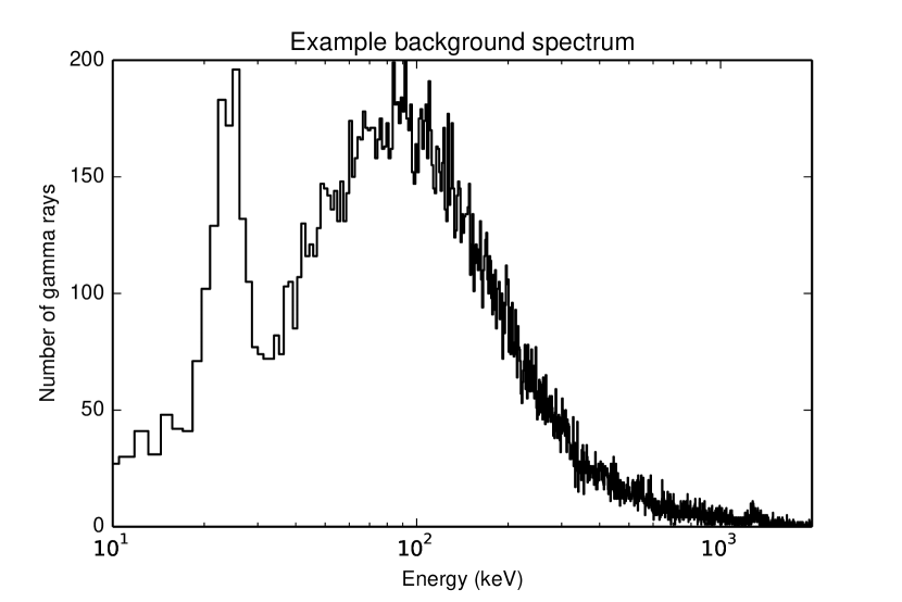
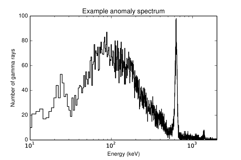
We collected our data using a $2\times 2$ inch Bridgeport Instruments cesium iodide spectrometer, a laptop, and a GPS unit. The spectrometer continuously recorded gamma rays and produced a 4,096-bin spectral histogram every two seconds; the laptop then recorded the histogram, time, and location. In typical conditions, 80–120 gamma rays were observed per histogram. An example spectrum, consisting of typical background gamma rays and summed over several hours, is shown in Fig. 2, while Fig. 3 shows a sample taken near a radioactive cesium-137 source.

Figure 1: A map of Pickle Research Campus with total gamma counts per second overlaid; counts are averaged over one month of data collection. Areas of elevated background include the radioactive materials storage facility at the northwest corner (A) and a cluster of large brick buildings near central campus (B). Figure reprinted from [4].

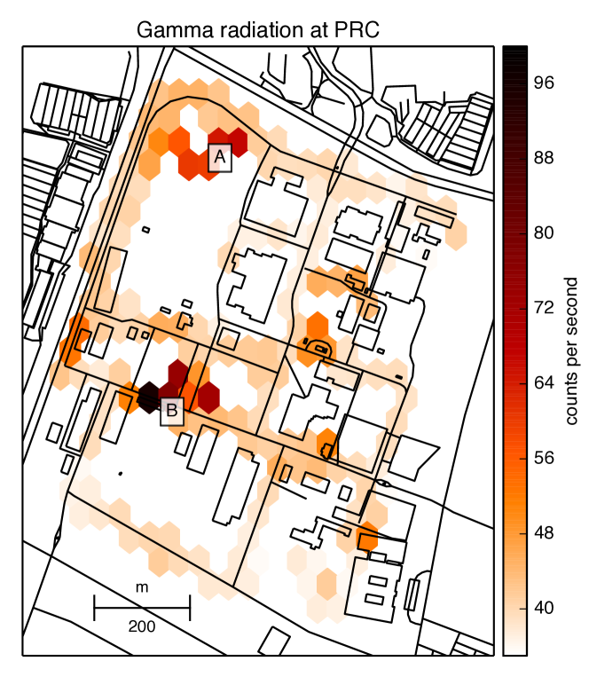
The dataset consists of once- or twice-daily drives through Pickle Research Campus (PRC) in the months of July and August 2012. The spectrometer and GPS unit were loaded onto a golf cart and driven around campus for roughly half an hour. Various spectral features at PRC, such as slightly-radioactive brick buildings and a radiological waste storage site, cause the area to have total background radiation levels which vary in space by about a factor of three; this variation is shown in Fig. 1. Cumulatively, the data includes roughly 18 hours of observations taken over 41 drives through campus on 30 different days.

In the course of our analysis we discovered that the dataset is contaminated: we used our Kolmogorov–Smirnov anomaly detection algorithm (Section 3.3) to compare each day to the previous day and identified days with unusual spectral differences, the largest of which is likely due to a downpour of 7 cm of rain the previous evening; rain can cause large variation in background spectra [5, 6]. In the rest of our analysis we excluded this day. (This was the largest rain event during the dry Texas summer, and the only to cause a noticeable anomaly.) This ensures our estimates of false positive rates (Section 3.3) do not contain true positives; we’ll instead use simulated sources of known size and location to test our algorithms. Future work may be able to account for rain-induced spectral changes using a model to relate precipitation rate and radon progeny deposited by rain [7].

3 Approach

To detect radioactive sources, two things are required. The first is a way to account for the natural spatial variation in background spectra (Section 3.1). The second is an anomaly detection algorithm which compares the background model with new observations and tests for statistically significant differences, producing a map of anomalous regions (Sections 3.2 and 3.3). Global false discovery control is essential to make the system practical, and the power of the procedure needs to be established for target radioactive sources.

The anomaly detection algorithm should use only the shape of the spectrum, not the total count rate, since observed count rates will vary widely depending on the detector, and a wide area monitoring system may use different sizes of detectors mounted on different vehicles at different heights. Also, like scram, our anomaly detection algorithm does not attempt to discriminate between benign and threatening anomalies, instead searching for any spectral change; users who need to search for specific sources can check anomalies using a source identification algorithm to locate specific isotopes [8, 9].

3.1 Background Radiation Model

The background spectrum arises from natural deposits of uranium, thorium, radon, and their decay products; these elements are more common in certain kinds of rock, such as granite, and hence the spectrum varies with local geology. This variation is usually smooth, though sudden changes in geology (such as a man-made granite wall) can cause sharp background changes. Similarly, different concrete mixes can have different mixtures of naturally radioactive materials, causing variation in the background emitted by concrete structures [10]. To avoid comparing new data to a heterogenous background, we divide the map into spatial cells and aggregate each cell’s data over several days to provide a background estimate.

Figure 2: A typical background radiation spectrum at Pickle Research Campus, comprising 32,173 gamma rays observed over several hours. Energy in kiloelectronvolts, in 4,096 bins, is shown on a logarithmic scale.

Figure 3: Spectrum recorded near a sample of radioactive cesium-137. The sharp peak on the right side of the plot, which stands out from the normal background, is the characteristic 662 keV gamma ray emitted in the decay of cesium-137.

3.2 Spectral Comparison Ratio Anomaly Mapping (scram)

The scram procedure was our initial attempt to perform anomaly detection [4]. It is based on the method of spectral comparison ratios of [3] and proceeds as follows: new spectra to be tested are aggregated in $250\times 250$ meter spatial cells (there are typically 12–15 such cells per day for the data analyzed here), downsampled from 4,096 energy bins to 8, and a $\chi^{2}$-like anomaly statistic $D^{2}$ calculated in each cell by comparing the 8-bin spectrum to spectra recorded on previous days in the same cell. Large values of $D^{2}$ relative to a reference distribution indicate elevated radioactive emissions in the corresponding cells.

scram makes various simplifying assumptions: count rates have a constant variance-to-mean ratio and background spectra are treated as exact. These assumptions imply that the $\chi^{2}$ distribution assumption underlying the test statistic $D^{2}$ does not hold; in particular, the distribution has a heavier tail than a $\chi^{2}$ [4]. We instead estimated the reference distribution of $D^{2}$ with a histogram of values of $D^{2}$ calculated for each of the 30 days of recorded data. This resulted in 399 observed test statistics, 12–15 per day, assumed to be from the null hypothesis that no genuine spectral difference exists. The 99th percentile of these values was $D^{2}=83$, which was then used as the cutoff for an $\alpha=0.01$ level test.

We consider a slightly modified version in this paper. Indeed, this cutoff value is not only variable, since it is estimated from a small sample, but it is also biased, since the dataset contains true positives, as mentioned earlier—rain-induced spectral changes produced anomalies across the entire map for one day. These outlying points inflated the $D^{2}$ cutoff. We excluded this day of observations from the dataset rather than attempting to isolate specific affected cells. We then repeated the procedure and calculated a parametric rather than a nonparametric cutoff: we fit a gamma distribution with probability density function

$$f(x)=\frac{\beta^{\alpha}}{\Gamma(\alpha)}x^{\alpha-1}e^{-\beta x}.$$

to the resulting 387 test statistics by maximum likelihood, and used its 99th percentile, $D^{2}=39.7$, as the cutoff. The gamma distribution includes the $\chi^{2}$ distribution as a special case but is more flexible, allowing in particular for the heavier tails caused by the assumption violations [4]. This parametric cutoff may be biased if the gamma reference distribution is not perfectly adequate, but it is also less sensitive to outliers and has lower estimation variance than the empirical cutoff of [4]. This lower rejection threshold has substantial impact on our power comparisons (see Section 4.1); the revised scram method is more sensitive than originally proposed.

Note that the nonparametric cutoff of [4] and the parametric cutoff calculated here are estimated from data, so they are variable. There is no standard analytical formula for the confidence interval of this estimate, so we used bootstrapping to estimate the uncertainty in this fit, using the following procedure [11]:

1. Re-sample at random and with replacement from the 387 test statistics.

2. Fit the gamma distribution to this new sample and calculate its 99th percentile.

3. Repeat 10,000 times.

The quantiles of the 10,000 repeat values of the cutoff are used to set the 95% basic bootstrap confidence interval of $[33.5,45.2]$, suggesting more data would be needed to more accurately choose a rejection threshold.

3.3 Kolmogorov–Smirnov Anomaly Detection

We developed an alternative approach that does not require empirical estimation of its rejection region, does not reduce its detection power by downsampling spectra, and does not require repeat days of observation to estimate the correlation between energy bins. Our approach uses a standard two-sample Kolmogorov–Smirnov (KS) test.

We again divide space into square cells and compare each cell to prior data. This approach treats gamma rays as draws from an underlying energy distribution, with the KS test checking if two samples come from the same distribution. Specifically, if $c_{j1},c_{j2},\dots,c_{j{n_{j}}}$ is a list of energies of $n_{j}$ gamma rays from distribution $j$, we let $\hat{F}_{j}(x)$ be their empirical cumulative distribution function—the proportion with energy less than or equal to $x$:

$$\hat{F}_{j}(x)=\frac{1}{n_{j}}\sum_{i=1}^{n_{j}}\mathbf{1}(c_{ji}\leq x),$$

where $\mathbf{1}(\cdot)$ is the indicator function, which is $1$ when its argument is true and $0$ otherwise. In our case, $\hat{F}_{1}(x)$ is the observed distribution of background gamma ray energies, and $\hat{F}_{2}(x)$ the distribution of a new observation. Then the test statistic is

$$D=\sup_{x}\left|\hat{F}_{1}(x)-\hat{F}_{2}(x)\right|.$$

When both samples are drawn from the same continuous distribution, $D$ has a null distribution which is easily approximated by standard statistical software packages. When they are not from the same distribution, $D$ tends to be large and the test rejects the null hypothesis, though as with all tests, its sensitivity decreases when the sample sizes $n_{1}$ and $n_{2}$ decrease.

The standard approximations for the KS test statistic null distribution assume that the data is drawn from a continuous probability distribution, so that no two observations have exactly the same value. However, our detector creates ties by discretizing energies into bins, biasing the test’s $p$ values to be larger than expected. We checked this by repeatedly simulating (resampling with replacement) from a single reference spectrum, then testing the simulated spectra against the reference spectrum; despite the spectra being draws from the same distribution, their $p$ values were not uniformly distributed but were skewed towards one. Biased $p$-values are problematic because they imply that the false positive rate of the test does not match the chosen significance level.

This problem could be solved by using a nonparametric permutation test, which simulates the null distribution of $D$ by repeatedly permuting the labels on the data. The gamma energies are gathered into a single list $c_{11},c_{12},\dots,c_{1{n_{1}}},c_{21},c_{22},\dots,c_{2{n_{2}}}$ and the following procedure is run:

1. Randomly shuffle the data list. Treat the first $n_{1}$ entries as samples from distribution 1 and the remaining $n_{2}$ entries as samples from distribution 2.

2. Calculate $D$ with the new samples.

3. Repeat at least 1,000 times. Calculate the $p$ value as the fraction of $D$ values larger than the unshuffled $D$.

The shuffling ensures there is no systematic difference between the two samples, so we can simulate the distribution of $D$ under the null hypothesis without any parametric assumptions. This eliminates the bias but requires time-consuming simulations. Alternatively, [12] describes a procedure for calculating an exact $p$ value in the case of ties, but for large sample sizes, the calculation is even slower than the permutation test. We next tested whether we could avoid these costly adjustments by calibrating the $p$ value threshold to get an approximate $\alpha=0.05$ test, and whether this test would have power equivalent to the permutation test.

We again used a simulation procedure, repeatedly resampling from a background distribution and injecting gamma rays from a cesium-137 source. First, we ran the simulation 10,000 times without the injected source, producing a null distribution, and calculated that 5% of the KS test’s $p$ values were below $p=0.067$, so we adopted this as our rejection threshold. Then we ran 1,000 simulations for each of several injected source sizes and compared the power of this adjusted KS test to the unadjusted permutation test. They were virtually identical, implying that the KS test with adjusted rejection threshold will suffice.

Finally, we checked how the bias manifested in real data. For every day of data, we compared the observations in each spatial cell to the previous day’s background measurements, then calculated the fraction of $p$ values below the unadjusted $\alpha=0.05$ threshold. We repeated this procedure for several cell sizes between $20\times 20$ and $100\times 100$ meters. Results are shown in Table 1. We found that for $20\times 20$m spatial cells, the proportion of test statistics below $\alpha=0.05$ was $0.052$, close to $0.05$. For large $100\times 100$m cells the $p$ values are biased downwards, with nearly 12% of $p$ values smaller than the $\alpha=0.05$ threshold.

This is the opposite of the bias we would expect from ties, and must come from some other source. To confirm this, we repeated the same simulation procedure but produced $p$ values using the permutation test. This test does not suffer from bias caused by ties, but Table 1 shows that its $p$ values become even more biased towards zero than the KS test’s as the cell size increases. This bias occurs because large spatial cells are spectrally heterogenous, so there are genuine differences to be detected. The permutation and unadjusted tests both pick this up and report more $p<0.05$ results, but for the latter this shift is partly balanced out by the opposite skew caused by ties. This suggests that the unadjusted KS test would be more useful in practice.

For the remainder of this paper we will therefore use the KS test, as it is much faster to compute, gives results which have good detection power, and has approximately the correct false positive rate when used with $20\times 20$m spatial cells. Larger cells would have larger sample sizes and greater power, but would have more false positives and be less able to localize small sources, so there is a tradeoff. When applied to other datasets with different detector sensitivity and spatial variability, the optimal cell size may differ.

Cell size (m)	Sample $n$	KS $\alpha$	Permutation $\alpha$
20	4604	0.052	0.064
40	2412	0.070	0.082
100	949	0.116	0.133

Table 1: For each size of spatial cell, the number of KS tests performed and the proportion of test statistics smaller than the nominal $\alpha=0.05$ level. The permutation test appears to have a higher false positive rate than the standard test using the asymptotic null distribution.

3.4 False Discovery Rate Detection

To produce an anomaly map, the data are divided into a spatial grid, with each cell’s background observation compared to the new data collected within the same cell, producing a $p$ value for each cell. To prevent many false detections due to multiple comparisons, the Benjamini–Hochberg procedure [13] is used to select a $p$ value cutoff to achieve a chosen false discovery rate, defined as the expected proportion of detections that are false out of all the detections. In this procedure, the cell $p$ values are sorted into ascending order, $p_{1}\leq p_{2}\leq\dots\leq p_{m}$, and the significance threshold is set to be the largest $p_{i}$ such that $p_{i}\leq iq/m$, where $q$ is the desired false discovery rate. This guarantees that, on average, the fraction of significant results which are statistical false positives will be $q$. We set $q=0.2$ for our simulations, but $q$ can be chosen to meet operational needs.

4 Results

We built on previous simulation tools [14] to create a set of power simulations to evaluate the performance of our anomaly detection algorithm. These simulations inject radioactive sources into observed data and account for the distance between source and detector, both with the normal $1/r^{2}$ falloff and with exponential attenuation due to gamma absorption in air, but not for physical obstacles, down-scatter, or shielding between the source and the detector. In this sense they are idealized; heavily shielded sources are harder to detect than the simulations suggest, and down-scatter will alter their spectra.

The count rate $\lambda$ for injected sources was based on the assumption that

$$\lambda\propto\frac{s}{r^{2}}\exp(-\mu d),$$

where $r$ is the distance to the source in meters, $s$ is its size in milliCuries and $\mu=0.0100029\,\text{m}^{-1}$ is the attenuation coefficient for cesium-137’s 660 keV gamma rays. The proportionality constant was determined from an experiment which placed a 0.000844 mCi cesium-137 source 0.05 meters away from our detector, recording 630 counts per second, so that ultimately, our source simulation model was:

$$\lambda(d,s)=\frac{s}{0.000844}\cdot 630\cdot\left(\frac{0.05}{r}\right)^{2}\cdot\exp\left(-\mu(r+0.05)\right).$$

To test our anomaly detection algorithm we must specify the anomalies of interest. The example in Fig. 3 shows the spectrum recorded near a sample of radioactive cesium-137; a sharp high-energy peak is apparent. Other anomalies may be different; iridium-192, for example, appears as several smaller peaks between 200 and 600 keV mixed in among the large background radiation smear. Statistical power depends on the type of radioactive source present, but because the KS test uses the cumulative distribution of gamma rays, it is sensitive to sharp peaks as well as spread-out differences in the spectrum. We will use cesium-137 for all our power simulations for consistency.

We also need to specify the background observation period based on the expected rate of change of the background spectrum. If the background is known to vary naturally over a period of a few days or weeks, we may use only the most recent few days to form the background to avoid using an outdated background estimate.

Despite this precaution, the selected background and observation periods may have genuine spectral differences, for example if rain changes the background spectrum. If these are statistically significant, then every simulation will result in a statistically significant result. To prevent this, we do not use data from the new observation period; instead, we sample with replacement the matching number of gamma rays from the background period in every spatial cell and inject the radioactive source into that simulated data. In practice, maps with anomalies reported everywhere would indicate a global phenomena, such as environmental change or calibration issue, and would be investigated accordingly.

4.1 Minimum Detectable Sources vs. Distance

Figure 4: Minimum source sizes detectable by our $2\times 2$ inch detector with 80% power as a function of distance, compared between KS tests and scram. The horizontal line indicates a 100 milliCurie source. KS tests are a clear improvement over scram, and the revised scram detection thresholds are a major improvement over the old version.

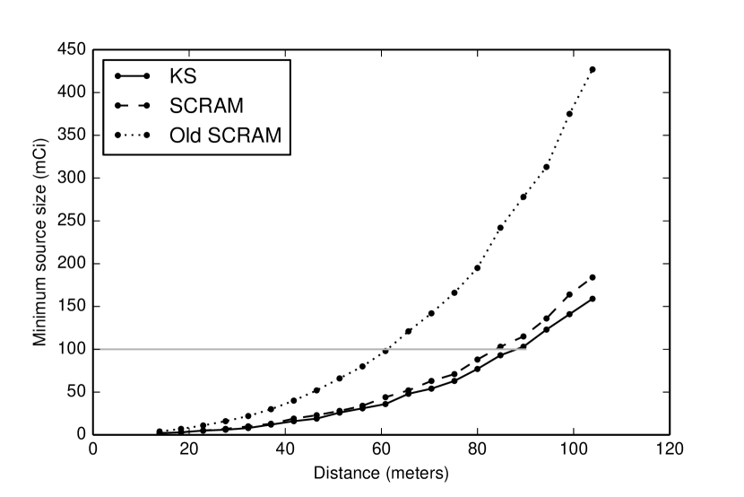
To compare the sensitivity of scram and KS tests for detecting small spectral anomalies, the first simulation determines the minimum radioactive source size necessary to trigger an alarm ($p<0.01$) with 80% power, at varying source distances from the detector. A 20-meter section of road at the PRC was selected as the test site and simulated cesium-137 sources injected at various distances from the road. KS tests and scram were run on the entire aggregated segment of road, using the previous seven days of observations as background data. (The detection threshold for scram was set by applying the procedure from Section 3.2 to 20-meter cells.) Fig. 4 shows the results; it provides the minimum detectable source at a given distance, and conversely the maximum distance at which a given source can be detected. For example, the horizontal line indicates the maximum distances at which a 100 milliCurie source can be detected by each algorithm at least 80% of the time. The old scram procedure detects it at about 65m, while the KS test detects it as far away as 90m, a substantial improvement in detection power. scram with the revised detection threshold is also an improvement, performing nearly as well as the KS tests.

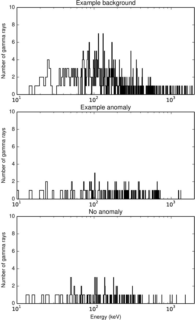
To illustrate the small amount of data that can be used to detect a source, Fig. 5 shows a background spectrum (about five seconds of observations), a simulated contaminated spectrum containing cesium-137 (about one second of observations), and a simulated spectrum with no contamination. Despite the small sample sizes, the KS test correctly identifies a statistically significant difference in the anomalous spectrum. (Recall that it detects differences in shape, not total number of counts.)

Because the KS test is simpler and more powerful than scram, the remainder of our power simulations will focus on the KS test. We do not show the equivalent power maps for scram.

Figure 5: At top, a simulated background spectrum comprising only 504 gamma rays drawn from the sample shown in Fig. 2. Center, a simulated spectrum comprising 97 background gamma rays and 50 from the cesium-137 sample shown in Fig. 3. Bottom, a simulated background of 116 gamma rays. Despite the small sample, the KS test correctly identifies the anomalous spectrum.

4.2 Minimum Detectable Source Maps

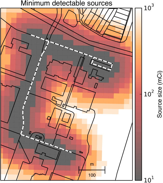
We also designed a minimum detectable source simulation tool. The user chooses a radioactive source, a minimum desired statistical power, a background observation period, and a new observation day. The simulation grids the data in the new observation day and sequentially injects a source at each grid location, recording the minimum source size required to have the desired power of detection in at least one grid cell. (Again, power is calculated by testing if the cell would be considered significant after false discovery rate control.) This produces a map of source sizes: the smallest detectable source size at each location.

An example map is shown in Fig. 6, which shows that with a week of daily background observations and only five minutes of new data, we have high power to detect fairly small radioactive sources along the detector’s route. More distant sources must be much larger to be reliably detected. An operator could use this map to understand the performance of the system and evaluate its ability to detect potential threats. This tool could also be adapted to plan detector routes through an area, identifying routes which efficiently cover the area of interest.

Figure 6: At each location, the smallest cesium-137 source that can be detected with 80% power by a detector which drove through once, using one full week of background data. The drive amounted to just five minutes of observations along the white dashed route.

4.3 Power Maps for Detecting Chosen Sources

Figure 7: Power to detect a 500 mCi cesium-137 source, injected at the blue dot, using one full week of background data (130 minutes of observations) and a single pass (22 minutes) of observations of the campus. The map shows only the northwest corner of PRC; each grid cell is $20\times 20$ meters, for a total of 245 cells, so the average cell contains just five seconds of observations of the source.

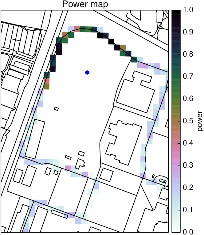
The next simulation we designed was interactive. The user selects a background observation period and a set of new data. The user then chooses a radioactive source and size and can click on a map to inject the source at any desired location in the new data. An anomaly is considered statistically significant if it passes the Benjamini–Hochberg procedure with a false discovery rate of 0.2, and the power measures how likely this is to occur in repeated simulations. One such simulation, using a 500 mCi cesium-137 source, is shown in Fig. 7. The source, placed in an empty field, is easily detected on the nearby road.

Because the map is interactive—parallelization means the simulations can run in just a few seconds—the user can explore likely locations for radioactive sources and determine if the available data is adequate to detect sources at these locations. If not, detectors could be rerouted to fill the gaps.

A non-interactive version of this map is easy to produce. After choosing a radioactive source and size, the source is injected into each grid cell, which is assigned a color proportional to the probability of detecting the source. (A source is considered to be detected if it results in a statistically significant anomaly anywhere else on the map, after the Benjamini–Hochberg procedure is applied.) If there is a specific target source of concern, this map shows where it would be best detected. We did not include an example here because the map looks like the inverse of Fig. 6—cells where the minimum detectable source is small have a higher power to detect the user-specified source.

5 Conclusions

KS tests promise to be a powerful, flexible, and simple alternative to scram for wide-area mapping and anomaly detection. More importantly, we have developed simulation tools that can guide the deployment of our anomaly detection algorithm in practice, showing that it can be made useful for real-world applications.

Comparisons against existing mobile source search systems, such as spectral comparison ratios [3] and the NaI–SS Radiation Search System [15], are difficult. These systems are not designed to monitor a wide area continuously for a long period of time, and their ability to detect small and distance sources has been evaluated using different sources and detectors than we possess. Nonetheless, we believe that our KS procedure is better suited to long-term radiation surveillance, particularly with the simulation tools we have developed to aid deployment.

Future work may expand our simulations and tests based on standard procedures such as those defined in ANSI N42.43–2006 or the Domestic Nuclear Detection Office’s Technical Capability Standard for Vehicle Mounted Mobile Systems. This would include simulating other common industrial and medical radioisotopes, as well as simulating shielded sources.

There are also opportunities for future improvement of our anomaly detection system. We could incorporate methods to detect specific isotopes or ignore known benign source types, such as common medical radioisotopes, building on previous work in isotope detection and identification [8, 9]. Additionally, we have not built a spatial model of spectra which allows borrowing of information between spatial cells. Two options are to smooth spectra in space [16] or to use a spatial false discovery procedure [17, 18]; it is not clear which will bring the greatest benefits, but either method would further improve sensitivity. We can also incorporate automated energy calibration [19] and rain detection [7] to better estimate background spectra with less variance.

References