Fast and Accurate Recurrent Neural Network Acoustic Models for Speech Recognition

Abstract

We have recently shown that deep Long Short-Term Memory (LSTM) recurrent neural networks (RNNs) outperform feed forward deep neural networks (DNNs) as acoustic models for speech recognition. More recently, we have shown that the performance of sequence trained context dependent (CD) hidden Markov model (HMM) acoustic models using such LSTM RNNs can be equaled by sequence trained phone models initialized with connectionist temporal classification (CTC). In this paper, we present techniques that further improve performance of LSTM RNN acoustic models for large vocabulary speech recognition. We show that frame stacking and reduced frame rate lead to more accurate models and faster decoding. CD phone modeling leads to further improvements. We also present initial results for LSTM RNN models outputting words directly.

Index Terms: speech recognition, acoustic modeling, connectionist temporal classification, CTC, long short-term memory recurrent neural networks, LSTM RNN.

1 Introduction

While speech recognition systems using recurrent and feed-forward neural networks have been around for more than two decades [1, 2], it is only recently that they have displaced Gaussian mixture models (GMMs) as the state-of-the-art acoustic model. More recently, it has been shown that recurrent neural networks can outperform feed-forward networks on large-scale speech recognition tasks [3, 4].

Conventional speech systems use cross-entropy training with HMM CD state targets followed by sequence training. CTC models use a “blank” symbol between phonetic labels and propose an alternative loss to conventional cross-entropy training. We recently showed that RNNs for LVCSR trained with CTC can be improved with the sMBR sequence training criterion and approaches state-of-the-art [5]. In this paper we further investigate the use of sMBR-trained CTC models for acoustic speech recognition and show that with appropriate features and the introduction of context dependent phone models they outperform the conventional LSTM RNN models by 8% relative in recognition accuracy. The next section describes the LSTM RNNs and summarizes the CTC method and sequence training. We then describe acoustic frame stacking as well as context dependent phone and whole-word modeling. The following section describes our experiments and presents results which are summarized in the conclusions.

Figure 1: Layer connections in unidirectional (top) and bidirectional (bottom) 5-layer LSTM RNNs.

2 RNN Acoustic Modeling Techniques

In this work we focus on the LSTM RNN architecture which has shown good performance in our previous research, outperforming deep neural networks.

RNNs model the input sequence either unidirectionally or bidirectionally  [6]. Unidirectional RNNs (Figure 1 top) estimate the label posteriors $y_{l}^{t}=p(l_{t}|x_{t},\overrightarrow{h_{t}})$ using only left context of the current input $x_{t}$ by processing the input from left to right and having a hidden state $\overrightarrow{h_{t}}$ in the forward direction. This is desirable for applications requiring low latency between inputs and corresponding outputs. Usually output targets are delayed with respect to features, giving access to a small amount of right/future context, improving classification accuracy without incurring much latency.

If one can afford the latency of seeing the entire sequence, bidirectional RNNs (Figure 1 bottom) estimate the label posteriors $p(l_{t}|x_{t},\overrightarrow{h_{t}},\overleftarrow{h_{t}})$ using separate layers for processing the input in the forward and backward directions. We use deep LSTM RNN architectures built by stacking multiple LSTM layers. These have been shown to perform better than shallow models for speech recognition [7, 8, 9, 3]. For bidirectional models, we use two LSTM layers at each depth — one operating in the forward and another operating in the backward direction over the input sequence. Both of these layers are connected to both the previous forward and backward layers. The output layer is also connected to both of the final forward and backward layers. We experiment with different acoustic units for the output layer, including context dependent HMM states and phones, both context independent and context dependent (Section 2.4). We train the models in a distributed manner using asynchronous stochastic gradient descent (ASGD) optimization technique allowing parallelization of training over a large number of machines on a cluster and enabling large scale training of neural networks [10, 11, 12, 13, 3]. The weights in all the networks are randomly initialized with a uniform (-0.04, 0.04) distribution. We clip the activations of memory cells to [-50, 50], and their gradients to [-1, 1], making CTC training stable.

2.1 CTC Training

The CTC approach [14] is a technique for sequence labeling using RNNs where the alignment between the inputs and target labels is unknown. CTC can be implemented with a softmax output layer using an additional unit for the blank label used to estimate the probability of outputting no label at a given time. “Blank” is similar to the “non-perceiving state” proposed earlier [15]. The output label probabilities from the network define a probability distribution over all possible labelings of input sequences including the blank labels. The network can be trained to optimize the total log probability of correct labelings for training data as estimated using the network outputs and forward-backward algorithm [16]. The correct labelings for an input sequence are defined as the set of all possible labelings of the input with the target labels in the correct sequence possibly with repetitions and with blank labels permitted between separate labels. The targets for CTC training can be efficiently and easily computed using finite state transducers (FSTs) as described in [5], with additional optional blank states interposed between the states of the sequence labels.

While conventional hybrid speech and handwriting recognition systems usually train from fixed alignments, the use of the forward-backward algorithm to reestimate network targets given the current model can equally be applied to conventional recurrent [17] or feed-forward networks [18] if no such alignment is available. These conventional realignment systems have followed the practice of choosing alignments to maximize the likelihood of the data under state sequence(s) that match the transcript, and use posteriors scaled by the label priors.

Hence, CTC differs from conventional modeling in two ways. First, the additional blank label relieves the network from making label predictions at a frame when it is uncertain. Second, the training criterion optimizes the log probability of state sequences rather than the log likelihood of inputs.

Whether using CTC with posteriors and a blank symbol or a conventional model with scaled posteriors, once the target posteriors are computed by the forward-backward algorithm, gradients of the Cross Entropy loss between the softmax outputs and the targets are backpropagated through the network.

As described in [5], one can use the standard beam search algorithm for speech decoding with CTC models, again allowing an optional blank state labels between the output labels in the search graph. In decoding, we only scale the blank label posterior by a constant scalar decided by cross-validation on a held-out set. We found that CTC models with phone labels do not require a language model weight to normalize acoustic model scores with respect to language model scores. However, CTC models with CD phone labels (Section 2.4) perform better with a weighting constant (2.1).

2.2 Sequence Discriminative Training

Cross-entropy and CTC criteria are suboptimal for the objective of word error rate (WER) minimization in ASR. A number of sequence-level discriminative training criteria incorporating the lexical and language model constraints used in speech decoding have been shown to improve the performance of DNN and RNN acoustic models bootstrapped with CE  [19, 20, 12, 21, 4] or CTC training criteria [5]. In this paper, we use the state-level minimum Bayes risk (sMBR) sequence discriminative training criterion [19] for improving accuracy of RNN acoustic models initialized with CE or CTC criterion. As discussed above and before [5], decoding with CTC models requires scaling the blank label posterior. We found that sMBR training can fix this scaling issue if we do not scale the blank label posterior while decoding an utterance to get numerator and denominator lattices during sMBR training. Alternatively, the blank label scaling can be baked into into the bias of the blank label output unit in the RNN model by adding negative log of the scale before starting sMBR training, just as the state priors can be baked into the softmax biases of conventional models before sequence training.

To summarize, after sequence discriminative training, the only difference between CTC and “conventional” models is the use of the blank symbol. Henceforth we use “CTC” to refer to these models (and their initial training using unscaled posteriors to generate alignments) and contrast them with “conventional” models which have no blank symbol, and which, in this paper, we train with fixed hard alignments.

2.3 Acoustic Features

We use 80-dimensional log mel filterbank energy features computed every 10ms on 25ms windows. We obtained significant improvements by increasing the number of filterbanks from 40 up to 80, but only present results for the latter.

In the past, we have observed that training with CTC is unstable, in that some training runs fail to converge. We found [5] that stability was improved by starting training using two output layers with CTC and the conventional CE loss, or initializing from a network whose LSTM layers had been pretrained using the CE loss. We suggest that this is because of the inherent arbitrariness of the alignment with CTC, which considers valid any alignment in which the target symbols are emitted in the correct order interspersed with an arbitrary number of blanks. One way of reducing the huge space of alignments is to reduce the number of input frames. This can be done by simply decimating the input frames, though to present the full acoustic information of the input signal, we first stack frames so that the networks sees multiple (e.g. 8) frames at a time but then decimate the frames so that we skip forward multiple frames (e.g. 3) after processing each such “super-frame”. This process is illustrated in Figure 2.

By decimating the frames in this manner, the acoustic model is able to process the full signal but acoustic model computation need only happen every 30ms. For a network of a fixed size this results in a dramatic reduction in the acoustic model computation and decoding time.

Figure 2: Stacking and subsampling of frames. Acoustic features are generated every 10ms, but are concatenated and down-sampled for input to the network: 8 frames are stacked for unidirectional (top) and 3 for bidirectional models (bottom).

2.4 Context-Dependent Phones

Previously CTC models [8, 5] used context independent outputs, yet it is well known that context dependent states outperform context independent models for conventional speech recognition systems, both GMM-based and neural-network hybrids. We argue that context dependency is an important constraint on decoding and provides a useful labeling for state outputs, so believe it should be useful for CTC models.

Previously, [22] it was shown that it is possible to build context dependent whole-phone models, and that for LSTM-HMM hybrid speech recognition, these models can give similar results to context dependent state models, provided that a minimum duration is enforced. We repeat that procedure, using the hierarchical binary divisive clustering algorithm of Young et al. [23] for context-tying. We use three frames of 40-dimensional log-mel filterbanks to represent each whole-phone instance. One tree per phone is constructed, with the maximum-likelihood-gain phonetic question being used to split the data at each node. On our training data we end up with 9287 CD phones.

As found before, enforcing a minimum duration for each phone was found to improve word error rates, and we again use a 10% cutoff of the training-set duration histogram as the minimum duration for each CD-phone for decoding of our conventional models. For CTC, no such duration model is imposed.

2.5 Word Acoustic Models

The combination of LSTM RNNs’ memory and CTC’s ability to learn an alignment between label and acoustic frame sequences, while relieving the network from having to label each frame by introducing the blank label, enables the use of longer duration modeling units. For instance, we can train acoustic models predicting whole words rather than phonemes. There have been previous studies using LSTM RNN CTC models for keyword spotting tasks with small vocabularies (e.g. 12 words [24]). In this paper, we investigate the effectiveness of word acoustic models trained over a large training set with various large vocabularies ranging from 7,000 to 90,000 words.

3 Experiments

3.1 Data & Models

We train and evaluate LSTM RNN acoustic models on hand-transcribed, anonymized utterances taken from real 16kHz Google voice search traffic. Our training set consists of 3 million utterances with average duration of about 4s. To achieve robustness to background noise and reverberant environments we synthetically distort each utterance in a room simulator with a virtual noise source. Noise is taken from the audio of YouTube videos. Each utterance is randomly distorted to get 20 variations. This “Multi-style training” also alleviates overfitting of CTC models to training data.

The test set’s 28,000 utterances are each distorted once with held-out noise samples. Evaluation uses a 5-gram language model pruned to 100 million $n$-grams. Rescoring word lattices with a larger $n$-gram model gives similar relative gains for all the acoustic models, therefore we only report results after first pass decoding. For all the experiments, we use a wide beam in decoding to avoid search errors and obtain the best possible performance.

For training networks with CE criterion using fixed alignments, the training utterances are force-aligned using an 85 million parameter DNN with 13522 CD HMM states. We explored variations of frame stacking and skipping as described in section 2.3. For the conventional unidirectional models’ inputs, we either stack 8 consecutive feature frames and skip 1 frame or present a single frame with a 5 frames delayed target — both approaches give similar results. For the bidirectional models, we only need to use a single frame input. For bidirectional CTC models, we stack 3 consecutive feature frames as input feature vector and skip 3 frames. For unidirectional CTC models, we stack 8 consecutive feature frames and skip 3 frames (Figure 2). We found longer context helps unidirectional models but is not needed for bidirectional models.

For CTC models, we obtained the best results with depth 5. Unidirectional models used 500 memory cells in each layer and bidirectional models had 300 memory cells for each direction in each layer. For the conventional models, we got the best results with 2 LSTM layers of 1000 cells each with a recurrent projection layer of 512 units.

3.2 Results & Discussion

Table 1 shows the word error rates (WERs) on the voice search task for various unidirectional and bidirectional LSTM RNN acoustic models trained with CE or CTC loss with CD HMM state, CI phone or CD phone labels. As can be expected from trying to learn with 3 state HMM labels, CTC CD state models do not perform well. The unidirectional CE CD phone model is marginally better than the corresponding CE CD state model. CTC CI phone models perform very similarly to CE CD state models. CTC CD phone models give significant improvements over CTC CI phone models – about 8% for unidirectional and 3.5% for bidirectional. Bidirectional models improve over unidirectional ones about 10% for CD state and CI phone models – while improving CTC CD phone models only 5%.

Labels CE (%) CTC (%) Uni Bi Uni Bi CD state 15.6 14.0 18.9 16.5 CI phone 15.5 14.1 CD phone 15.5 14.3 13.6

Table 1: WERs for conventional and CTC initialization of LSTM RNN acoustic models.

Table 2 shows the results for sequence discriminative training of these initial CE/CTC models with sMBR loss. We can see that sMBR training consistently improves all of the models initially trained with CE or CTC loss about 10% relative. We obtain best results with CTC CD phone models outperforming the second best model about 8% for unidirectional and 4% for bidirectional model.

Labels Initialization +sMBR Method Uni Bi Uni Bi CD state CE 15.6 14.0 14.0 12.9 CI phone CTC 15.5 14.1 14.2 12.7 CD phone CTC 14.3 13.6 12.9 12.2

Table 2: WERs (%) for sequence-trained LSTM RNN models.

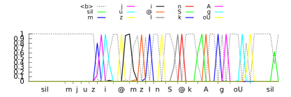
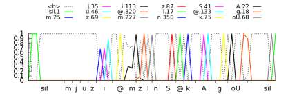
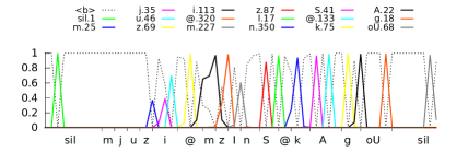
Figure 3 shows label posteriors estimated by various CTC phone and CD phone models. It can be seen that spikes for the label posteriors do not correspond to the DNN alignment and differ between the models. Unidirectional models delay their output labels by about 300 milliseconds. As can be expected, bidirectional models make better predictions. The models are not good at modeling silence labels. Sequence discriminative training changes posteriors, but not the spike positions.

(a) unidirectional phone CTC + sMBR

(b) unidirectional CD phone CTC

(c) unidirectional CD phone CTC + sMBR

(d) bidirectional CD phone CTC + sMBR

Figure 3: Label posteriors estimated by various LSTM RNN models plotted against fixed DNN frame level alignments shown only for labels in the alignment on a heldout utterance ‘museums in Chicago’. <b> refers to the blank label.

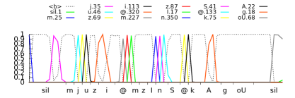
While learning an alignment in conventional GMM-HMM systems and DNN-HMM hybrid systems has been shown to work well, learning a conventional alignment without blank label using LSTM RNNs does not work well. Figure 4 shows label posteriors estimated using a unidirectional LSTM RNN CD phone model trained with CTC loss with no blank label allowed between CD phone labels. The model has learned an arbitrary alignment. Having a memory as in RNN models in contrast to memoryless feed forward neural networks means the model can delay its outputs instead of making decisions using only local temporal information. Therefore, the model learns an alignment where it chooses to adjust its labeling according to its certainty for a label given the input. This results in an arbitrary alignment where some labels are repeated more than others depending on the input. Note that using a hybrid approach with a prior cannot fix this issue.

Figure 4: Label posteriors for a unidirectional LSTM RNN model with conventional alignment – no blank label.

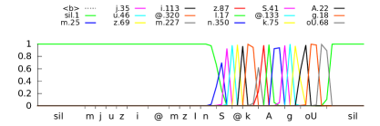
We have experimented with CTC word models with various vocabulary sizes where the output layer directly predicts words rather than phonemes. We have used two different vocabularies with the most frequent 7,000 ($\geq 150$ exemplars) or 25,000 ($\geq 20$ exemplars) words from the training data transcripts. Table 3 shows WERs for bidirectional CTC word acoustic models as calculated edit distance between reference word sequence and predicted word sequence where the word with highest probability is taken ignoring repetitions and the blank label with no language model or decoding. We have also experimented with 90k vocabulary CTC word models, and note that the bidirectional model gives a 25% lower WER than the unidirectional model.

Vocabulary OOV WER (%) In vocab. WER (%) 25k Word 4.8 19.5 14.5 7k Word 13 26.8 11.8

Table 3: LSTM RNN CTC word acoustic models. The WERs and out of vocabulary (OOV) rates for word models are on heldout data with no decoding or language model. WERs in the last column are computed ignoring utterances containing OOVs.

Figure 5 shows label posteriors estimated by the bidirectional CTC models with 7k and 90k vocabulary for a heldout utterance. We plot the posteriors for all the labels that were above 0.05 probability at any time. The words ’dietary’ and ’nutritionist’ are OOV for the 7k vocabulary. It is interesting to see that the models make spiky predictions even with a large vocabulary and the predictions for confused words are output at the same time. Although these two models have very similar spike positions for the words, they are different for the 25k model.

(a) 7k vocabulary

(b) 90k vocabulary

Figure 5: ‘To become a dietary nutritionist what classes should I take for a two year program in a community college’

4 Conclusions

In this work we have shown a number of improvements to recurrent network acoustic models. The use of longer-term feature representations, processed at lower frame rates brought stability to the convergence of CTC training of models with blank symbol outputs while also resulting in a considerable reduction in computation. After sequence training, such models are found to perform better than previous acoustic models. Performance of the blank-symbol acoustic models was further improved by the introduction of context-dependent phonetic units, with the result that these models now outperform conventional sequence trained LSTM-hybrid models. We have also shown that we can train word level acoustic models to achieve reasonable accuracy on medium vocabulary speech recognition without using a language model.

References

- [1] A. Robinson, M. Hochberg, and S. Renals, “The use of recurrent networks in continuous speech recognition,” in Automatic Speech and Speaker Recognition, K. K. P. C.-H. Lee, F. K. Soong, Ed. Norwell, MA, USA: Kluwer Academic Publishers, 1996, pp. 233–258.
- [2] H. Bourlard and N. Morgan, Connectionist speech recognition. Kluwer Academic Publishers, 1994.
- [3] H. Sak, A. Senior, and F. Beaufays, “Long Short-Term Memory Recurrent Neural Network Architectures for Large Scale Acoustic Modeling,” in INTERSPEECH 2014, 2014.
- [4] H. Sak, O. Vinyals, G. Heigold, A. Senior, E. McDermott, R. Monga, and M. Mao, “Sequence discriminative distributed training of long short-term memory recurrent neural networks,” in Interspeech, 2014.
- [5] H. Sak, A. Senior, K. Rao, O. Irsoy, A. Graves, F. Beaufays, and J. Schalkwyk, “Learning acoustic frame labeling for speech recognition with recurrent neural networks,” in IEEE International Conference on Acoustics, Speech, and Signal Processing (ICASSP), 2015.
- [6] M. Schuster and K. K. Paliwal, “Bidirectional recurrent neural networks,” Signal Processing, IEEE Transactions on, vol. 45, no. 11, pp. 2673–2681, 1997.
- [7] F. Eyben, M. Wollmer, B. Schuller, and A. Graves, “From speech to letters using a novel neural network architecture for grapheme based ASR,” in Automatic Speech Recognition & Understanding, 2009. ASRU 2009. IEEE Workshop on. IEEE, 2009, pp. 376–380.
- [8] A. Graves, A. Mohamed, and G. Hinton, “Speech recognition with deep recurrent neural networks,” in IEEE International Conference on Acoustics, Speech, and Signal Processing (ICASSP), 2013.
- [9] A. Graves, N. Jaitly, and A. Mohamed, “Hybrid speech recognition with deep bidirectional LSTM,” in Automatic Speech Recognition and Understanding (ASRU), 2013 IEEE Workshop on. IEEE, 2013, pp. 273–278.
- [10] Q. Le, M. Ranzato, R. Monga, M. Devin, K. Chen, G. Corrado, J. Dean, and A. Ng, “Building high-level features using large scale unsupervised learning,” in International Conference on Machine Learning, 2012, pp. 81–88.
- [11] J. Dean, G. Corrado, R. Monga, K. Chen, M. Devin, Q. Le, M. Mao, M. Ranzato, A. Senior, P. Tucker, K. Yang, and A. Ng, “Large scale distributed deep networks,” in Advances in Neural Information Processing Systems (NIPS), 2012.
- [12] H. Su, G. Li, D. Yu, and F. Seide, “Error back propagation for sequence training of context-dependent deep networks for conversational speech transcription,” in IEEE International Conference on Acoustics, Speech, and Signal Processing (ICASSP), 2013, pp. 6664–6668.
- [13] G. Heigold, V. Vanhoucke, A. Senior, P. Nguyen, M. Ranzato, M. Devin, and J. Dean, “Multilingual acoustic models using distributed deep neural networks,” in IEEE International Conference on Acoustics, Speech, and Signal Processing (ICASSP), vol. 1, Vancouver, Canada, Apr. 2013.
- [14] A. Graves, S. Fernández, F. Gomez, and J. Schmidhuber, “Connectionist temporal classification: Labelling unsegmented sequence data with recurrent neural networks,” in Proceedings of the 23rd International Conference on Machine Learning. ACM, 2006, pp. 369–376.
- [15] N. Morgan, H. Bourlard, S. Greenberg, and H. Hermansky, “Stochastic perceptual auditory-event-based models for speech recognition,” in ICSLP, 1994.
- [16] L. R. Rabiner, “A tutorial on hidden Markov models and selected applications in speech recognition,” Proceedings of the IEEE, vol. 77, no. 2, pp. 257–286, Feb. 1989.
- [17] A. Senior and A. Robinson, “Forward-backward retraining of recurrent neural networks,” in NIPS, 1994.
- [18] A. Senior, G. Heigold, M. Bacchiani, and H. Liao, “GMM-free DNN training,” in Proc. ICASSP, 2014.
- [19] B. Kingsbury, “Lattice-based optimization of sequence classification criteria for neural-network acoustic modeling,” in IEEE International Conference on Acoustics, Speech, and Signal Processing (ICASSP), Taipei, Taiwan, Apr. 2009, pp. 3761–3764.
- [20] B. Kingsbury, T. N. Sainath, and H. Soltau, “Scalable minimum Bayes risk training of deep neural network acoustic models using distributed Hessian-free optimization,” in Interspeech, 2012.
- [21] K. Veselý, A. Ghoshal, L. Burget, and D. Povey, “Sequence-discriminative training of deep neural networks,” in Interspeech, 2013.
- [22] A. Senior, H. Sak, and I. Shafran, “Context dependent phone models for LSTM RNN acoustic modelling,” in IEEE International Conference on Acoustics, Speech, and Signal Processing (ICASSP), 2015.
- [23] S. Young, J. Odell, and P. Woodland, “Tree-based state tying for high accuracy acoustic modelling,” in Proc. ARPA Human Language Technology Workshop, 1994.
- [24] S. Fernández, A. Graves, and J. Schmidhuber, “An application of recurrent neural networks to discriminative keyword spotting,” in ICANN, 2007, pp. 220–229.