1 Introduction

The present global PDF analyses (e.g. NNPDF3.0 [1], MMHT2014 [2], CT14 [3]) find that there is a large uncertainty in the low $x$ behaviour of the gluon distribution. There is a lack of very low $x$ data, particularly at low scales. Moreover, the gluon is determined at low $x$ mainly by the DGLAP evolution of deep inelastic scattering, that is, not from a direct measurement, but rather from the derivative $\mathrm{d}F_{2}/\mathrm{d}\ln Q^{2}$. As a result, at low scales, the uncertainty on the gluon PDF is large for $x\lower 3.01385pt\hbox{$\;\stackrel{{\scriptstyle\textstyle<}}{{\sim}}\;$}10^{-3}$. On the other hand, the HERA data on diffractive vector meson photoproduction [4, 5, 6, 7, 8, 9, 10, 11, 12, 13, 14, 15], $\gamma p\to V+p$ and the LHC data on the exclusive processes $pp\to p\,V\,p$ [16, 17, 18] where $V=J/\psi$ or $\Upsilon$, and $p\,\mathrm{Pb}\to p\,V\,\mathrm{Pb}$ [19], sample directly the gluon distribution down to $x\sim 10^{-5}$. For a review of exclusive vector-meson production at the LHC see, for example, Ref. [20].

However, $J/\psi$ and $\Upsilon$ data are not used in the global PDF analyses. One reason is that the corresponding cross sections are described by non-diagonal (skewed) analogues of the PDFs, namely generalised parton distributions (GPDs), due to the different masses of the incoming photon and the outgoing $V$ meson [21]. The GPDs can be related to the PDFs via the Shuvaev transform in the low $\xi$ region [22]. In this work, following [23], we make the physically motivated assumption that the input distribution has no singularities in the right-half Mellin-$N$ plane which implies that this relation holds at NLO to accuracy $\mathcal{O}(\xi)$. Another reason is the dependence of the theoretical predictions on the choice of the factorisation scale, $\mu_{F}$. This problem has two independent parts. One part has a technical nature and the other is more physical. Let us discuss them in turn. First, the ‘technical’ problem, which is related to the convergence of the perturbative expansion at low $\xi$ and low scales. A good illustration is that the NLO amplitude for the exclusive high-energy $\gamma p\to J/\psi+p$ process [24] was shown to yield a cross section which varies by up to an order of magnitude for a reasonable variation of $\mu_{F}$. This problem was emphasised recently by Wagner et al. [25]. The strong scale dependence arises because in the DGLAP evolution of low $\xi$ GPDs the probability of emitting a new gluon is strongly enhanced by the large value of $\ln(1/\xi)$. Indeed, the mean number of gluons in the interval $\Delta\ln\mu_{F}$ is [26]

$$\langle n\rangle\;\simeq\;\frac{\alpha_{s}N_{C}}{\pi}\;\ln(1/\xi)\;\Delta\ln\mu_{F}^{2}\,,$$ (1)

leading to a value of $\langle n\rangle$ up to about 8, for the case $\ln(1/\xi)\sim 8$ with the usual $\mu_{F}$ scale variation interval from $\mu_{F}/2$ to $2\mu_{F}$. In contrast, the NLO coefficient function allows for the emission of only one gluon. Therefore we cannot expect compensation between the contributions coming from the GPD and the coefficient function as we vary the scale $\mu_{F}$. (At large $\xi$ the compensation is much more complete and provides reasonable stability of the predictions to variations of the scale $\mu_{F}$.) In Section 2, we use the NLO contribution to fix a choice of the factorisation scale for the LO part of the amplitude, which allows the $\ln(1/\xi)$ corrections to be resummed.

The second or ‘physical’ reason why there is a strong scale dependence of $J/\psi$ and $\Upsilon$ photoproduction is due to ‘defects’ in the presently available PDF sets which are obtained in the DGLAP global analyses of deep inelastic and related hard scattering data. That is, our studies indicate that there is a strong scale dependence in vector-meson photoproduction caused by the unexpectedly small LO contribution in comparison with the NLO correction. This occurs due to the very low input gluon density in the low $x$ domain obtained in the recent global PDF analyses. We conclude that at the input scale, the low $x$ gluon density is underestimated in comparison with that for quarks. The crucial observation is that the number of input gluons (which is parametrised freely in the global analyses) is found to be much less than the number of such gluons emitted by quarks — or, to be more precise, gluons associated with the quark (each quark carries a gluon field created by its colour charge). With the present global partons the NLO sea quark contribution to $V$ meson photoproduction grows with decreasing $x$ faster than the input gluons. As a result, at sufficiently high energy, the quark component of the NLO correction to $V$ photoproduction approximately cancels the main LO contribution which is due only to the gluon density. Therefore a small variation of the scale in the NLO component leads to a strong variation of the predicted cross section.

Recently the LHCb Collaboration have presented data for open charm and beauty production in the forward direction [27, 28]. These data sample approximately the same kinematic domain as exclusive vector meson production; actually the $x$ values are slightly larger, and the scale for beauty production is also larger. It was shown in [29, 30] that the data can be reproduced by NLO QCD using the present global PDFs. Note, however, that again there is a large sensitivity to the choice of factorization scale. Indeed, to reproduce the data one needs to take a scale approximately a factor of two larger than the natural choice $\mu_{F}=\sqrt{Q^{2}+m^{2}_{Q}}$. Since the optimal or appropriate scale for open heavy-quark production is not known at present, these data do not yet reliably determine the low $x$ gluon at low scales. In the present paper we focus on exclusive vector-meson production. Moreover, our goal is not to present a new global PDF analysis or an explicit determination of the low $x$ gluon, but rather to study the possibility to reduce the scale dependence of the prediction, to study the qualitative structure of the NLO amplitude and to give hints of the consequences for the behaviour of the low $x$ gluon at low scales.

In Section 2 we consider the NLO contribution originating from the light quark (singlet) GPD. We show that this part of the NLO amplitude allows us to choose a factorisation scale which sums the $\ln(1/\xi)$ enhanced contributions inside the GPD. The remaining part of the NLO contribution has no large $\ln(1/\xi)$ factors, and, as shown in Section 3.2, the compensation between the scale dependence of the GPDs and of the coefficient functions for $\Upsilon$ production makes the NLO result sufficiently stable for the data to be included in global parton analyses (just as for the predictions of processes at larger $x$). The study of the $J/\psi$ photoproduction in Section 3.1 suggests that the gluon density obtained in the existing PDF analyses is too small at low $x$ and low scale. In Section 4 we present our conclusions.

2 NLO corrections and the choice of $\mu_{F}$

Our aim in this section is to show how knowledge of the NLO contribution for $\gamma p\to V+p$ allows us to sum the $\ln(1/\xi)$ enhanced contributions by a particular choice of $\mu_{F}$ in the LO part of the amplitude (and correspondingly in the NLO coefficient function), which, in turn, reduces the factorisation scale dependence of the predicted cross section. We outline the procedure in Section 2.2, but first we comment on the NLO formalism.

2.1 NLO formalism for $\gamma p\to V+p$

The NLO formalism for $\gamma p\to Vp$ has been presented in [24]. However, before we can apply it to describe the high energy $V$ photoproduction data, we must note one important correction.

The LO partonic amplitude, $\mathcal{A}_{g}^{(0)}(x/\xi)$, for the subprocess $\gamma+(gg)\to V$, can be calculated by considering the fusion of a photon with a pair of on-shell gluons with zero transverse momentum and physical, transverse, polarisations. If we use dimensional regularisation with $D=4+2\epsilon$ (as in [24]) to regularize the ultraviolet (UV) and infrared (IR) divergences, then the result is given, before dividing by the number of physical transverse polarisations of the incoming gluon, by

$$\mathcal{A}_{g}^{(0)}(x/\xi)=\alpha_{s}2(1+\epsilon)\,.$$ (2)

In $D$ dimensions, there are $D-2=2+2\epsilon$ possible transverse directions. Since the entire calculation must be performed in $D$ dimensions, to properly average over the polarisation of the incoming gluon, we must divide (2) by this factor, and not simply by 2. Therefore for the LO partonic amplitude we obtain, contrary to [24] (prior to the first erratum),

$$\mathcal{A}_{g}^{(0)}(x/\xi)=\alpha_{s}\,.$$ (3)

The difference of a factor of $(1+\epsilon)$ does not alter the finite LO result (as $\epsilon$ is taken to zero) but does lead to a different NLO result due to the differing counter-terms. Indeed, the extra factor $(1+\epsilon)$ presented in [24] generates extra terms $\sim\epsilon/\epsilon$ in the counter-terms, $\Delta$, giving them a form

$$\Delta=\dots\left(\frac{1}{\hat{\epsilon}}+1+\ln\left(\frac{\mu_{F}^{2}}{\mu^{2}}\right)\right),$$

where $1/\hat{\epsilon}=1/\epsilon+\gamma_{E}-\ln(4\pi)$ and $\gamma_{E}$ is the Euler-Mascheroni constant. However, with the LO partonic amplitude (3) we instead obtain counter-terms containing

$$\Delta=\dots\left(\frac{1}{\hat{\epsilon}}+\ln\left(\frac{\mu_{F}^{2}}{\mu^{2}}\right)\right).$$

It is precisely this alteration to the counter-terms which leads us to a different NLO finite result. This result agrees with that of [24] with both errata.

The details of our recalculation of the NLO result will be published separately [33]. Here we simply state the final result for the high-energy limit of the NLO part of the amplitude. In the high-energy approximation, $W^{2}\gg M_{V}^{2}$ (where $W$ is the c.m. energy of the incoming $\gamma p$ system and $M_{V}$ the mass of the vector meson), the imaginary part of the amplitude dominates and the leading contribution to the NLO correction comes from the region $\xi\ll\left|x\right|\ll 1$. The matrix element is given by

$$A^{(1)}(\xi,\mu_{F}) \approx -\mathrm{i}\pi\;C^{(0)}_{g}\Bigg{[}\frac{\alpha_{s}(\mu_{R})N_{c}}{\pi}\ln\left(\frac{m^{2}}{\mu_{F}^{2}}\right)\intop_{\xi}^{1}\frac{\mathrm{d}x}{x}F_{g}(x,\xi,\mu_{F})$$ (4)

$$+\;\;\frac{\alpha_{s}(\mu_{R})C_{F}}{\pi}\ln\left(\frac{m^{2}}{\mu_{F}^{2}}\right)\intop_{\xi}^{1}\mathrm{d}x\left(F_{S}(x,\xi,\mu_{F})-F_{S}(-x,\xi,\mu_{F})\right)\Bigg{]}\,.$$

Here $m$ is the mass of the $c$ (for $J/\psi$) or $b$ (for $\Upsilon$) quark and

$$F_{g}(x,\xi,\mu)\; =\;\sqrt{1-\xi^{2}}H_{g}(x,\xi,\mu),$$ (5)

$$F_{S}(x,\xi,\mu)\; =\;\sqrt{1-\xi^{2}}H_{S}(x,\xi,\mu),$$ (6)

(for this unpolarised, forward process) with $H_{g}$, $H_{S}$ the gluon and quark singlet GPDs, respectively. The GPDs can be calculated from the diagonal PDFs, $q(x,\mu)$, $\bar{q}(x,\mu)$ and $g(x,\mu)$, via the Shuvaev transforms:

$$H_{S}(x,\xi,\mu)\; =\;\sum_{q=u,d,s}H_{q}(x,\xi,\mu)-H_{q}(-x,\xi,\mu),$$ (7)

$$H_{q}(x,\xi,\mu)\; =\;\begin{dcases}\int_{-1}^{1}\>{\rm d}x^{\prime}\left[\frac{2}{\pi}\>{\rm Im}\>\int_{0}^{1}\>\frac{{\rm d}s}{y(s)\>\sqrt{1-y(s)x^{\prime}}}\right]\>\frac{{\rm d}}{{\rm d}x^{\prime}}\left(\frac{q(x^{\prime},\mu)}{|x^{\prime}|}\right),&x\geq 0\\ \int_{-1}^{1}\>{\rm d}x^{\prime}\left[\frac{2}{\pi}\>{\rm Im}\>\int_{0}^{1}\>\frac{{\rm d}s}{y(s)\>\sqrt{1-y(s)x^{\prime}}}\right]\>\frac{{\rm d}}{{\rm d}x^{\prime}}\left(\frac{\bar{q}(x^{\prime},\mu)}{|x^{\prime}|}\right),&x<0\end{dcases}$$ (8)

$$H_{g}(x,\xi,\mu)\; =\;\int_{-1}^{1}\>{\rm d}x^{\prime}\left[\frac{2}{\pi}\>{\rm Im}\>\int_{0}^{1}\>\frac{{\rm d}s(x+\xi(1-2s))}{y(s)\>\sqrt{1-y(s)x^{\prime}}}\right]\>\frac{{\rm d}}{{\rm d}x^{\prime}}\left(\frac{g(x^{\prime},\mu)}{|x^{\prime}|}\right)\>,$$ (9)

where

$$y(s)=\frac{4s(1-s)}{x+\xi(1-2s)}\,,$$ (10)

with an accuracy ${\cal O}(\xi)$, see Ref. [23]. Expressions (8) and (9) were used not only for the asymptotic NLO amplitude, (4), but also for the full expression for the complete NLO amplitude used in the numerics presented below. The LO coefficient function,

$$C_{g}^{(0)}=\alpha_{s}(\mu_{R})\frac{4\pi\sqrt{4\pi\alpha}e_{q}(e_{V}^{*}e_{\gamma})}{N_{c}\,\xi}\left(\frac{\langle O_{1}\rangle_{V}}{m^{3}}\right)^{1/2},$$ (11)

where $e_{i}$ are polarisation vectors and $\langle O_{1}\rangle_{V}$ is the NRQCD (non-relativistic QCD) matrix element of the $c{\bar{c}}\to J/\psi$ (or $b{\bar{b}}\to\Upsilon$) transition. In order to have a small relativistic correction to $\langle O_{1}\rangle_{V}$, we have to calculate the Feynman diagrams assuming that the charm/bottom-quark line has mass $m=M_{V}/2$ where $V=J/\psi,\Upsilon$ [34].

One can see directly from the high energy, leading $\ln(1/\xi)$, limit, given in (4), that for the choice $\mu_{F}=m$ the asymptotic limit of the quark NLO contribution vanishes. It is this observation that will allow us (in Section 2.3) to claim that a suitable value for the factorisation scale in leading logarithm terms is $\mu_{F}=m$.

Before we show how the NLO contribution allows us to fix the scale $\mu_{F}$ in the LO term, it is informative to first recall its structure and introduce the notation in terms of the LO prediction.

2.2 General procedure

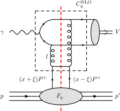
We start with the LO contribution to $\gamma p\to V+p$. It is sketched in Fig. 1(a), and the amplitude is given by the convolution

$$A^{(0)}(\xi,\mu_{F})\;=\int^{1}_{-1}\frac{dx}{x}C^{(0)}_{a}(x/\xi)F_{a}(x,\xi,\mu_{F})~{}\equiv~{}C^{(0)}_{a}\otimes F_{a}(\mu_{F})\,,$$ (12)

where the sum over $a=q,g$ is understood and $C^{(0)}_{q}=0$ for this process. The coefficient function $C^{(0)}_{g}$ is calculated using the non-relativistic vector meson wave function. In general, the relativistic corrections are not small for the $J/\psi$ case. These corrections should be considered together with the three parton ($c\bar{c}+g$) component of the wave function; that is, accounting for the rôle of gluons which provide the interaction between charm quarks. For this process, it was shown by Hoodbhoy [34] that the consistent treatment of relativistic corrections may, to good accuracy, be effectively accounted for by choosing, in the non-relativistic formula, the charm quark mass $m_{c}=M_{J/\psi}/2$. After this, the remaining part of the correction is quite small (a few percent only). So, we may use the non-relativistic $J/\psi$ wave function with $m_{c}=M_{J/\psi}/2$, to obtain a result with good accuracy.

We return to discuss $V=J/\psi$ or $\Upsilon$. At LO the coefficient function $C^{(0)}_{g}$ does not depend on $\mu_{F}$, whereas the low $x$ gluon distribution $F_{g}$ depends strongly on the scale. In other words, based on (12), the exclusive $V$ data measure $g(x,\mu_{F})$, but we do not know the value of the scale at which it has been determined. How does this scale freedom arise? To obtain the LO result the coefficient function – the upper box in Fig. 1(a) – is calculated with on-mass-shell gluons with transverse momenta $l_{t}=0$. In this collinear approach the factorisation scale $\mu_{F}$ acts effectively as the ultraviolet (UV) cutoff of the logarithmic integral $\int dl^{2}_{t}/l^{2}_{t}\propto\ln\mu^{2}_{F}$ over the gluon transverse momentum in the gluon loop of Fig. 1(a). Formally, in the LO collinear factorisation approach the value of $\mu_{F}$ is not known. In principle, the full result does not depend on $\mu_{F}$ since the higher-order, NLO, NNLO, …, corrections compensate the effect of variations of $\mu_{F}$. However, in reality the perturbative series is truncated and the compensation may not be sufficient to provide the scale stability of the theoretical prediction.

On the other hand, we can go beyond the collinear logarithmic approximation by computing the $l_{t}$ integral accounting for the $l_{t}$ dependence of the hard $\gamma+gg\to V$ matrix element, $\cal{M}$, shown in the upper box of Fig. 1(a). In comparison with the coefficient function (calculated with $l_{t}=0$) now the $l_{t}$ and $l^{2}$ dependence of $\cal{M}$ is included explicitly, and provides the UV convergence of the integral over $l_{t}$. Formally, in collinear factorisation the difference between the pure logarithmic ($\ln\mu_{F}^{2}$) evaluation and the precise calculation of the gluon $l_{t}$ integral is treated as part of the NLO correction. This part of the NLO correction is of kinematic origin and is usually quite large. Fortunately, it can be moved into the LO component of the amplitude, noticeably reducing the remaining NLO correction.

Instead of performing an independent calculation which accounts for the $l_{t}$ dependence, we can remain within the collinear approach and determine the value of the $l_{t}$ integral given that the NLO coefficient function $C^{(1)}_{q}$ of Fig. 1(b) is known. Indeed, Fig. 1(b) is the only diagram for the quark NLO coefficient function. In this approach the incoming quarks are assumed to be on-mass-shell and with zero transverse momenta but the loop integral over $l$, which contains the $l_{t}$ dependence, is calculated exactly. Since this is the same integral as that which occurs in Fig. 1(a) we can use the result for $C^{(1)}_{q}$ to obtain a precise value, $J$, of the corresponding integral in the LO amplitude of Fig. 1(a). After this we choose a scale $\mu_{F}=\mu_{0}$ which mimics the precise $l_{t}$ integration. That is, with a scale choice satisfying $\ln\mu^{2}_{0}=J$ we have moved a large contribution from NLO to LO, and can continue to work in the conventional collinear approach, but now with a smaller NLO correction.

Figure 1: (a) The LO contribution to $\gamma p\to V+p$, showing the convolution (12). (b) The NLO quark contribution. For these graphs all permutations of the parton lines and coupling of the gluon lines to the heavy-quark pair are to be understood. Here $P\equiv(p+p^{\prime})/2$ and $l$ is the loop momentum.

2.3 Transfer of part of the NLO to the LO contribution

Since the above observation is crucial, let us demonstrate the procedure in more detail. At NLO level the LO+NLO amplitude at some factorisation scale $\mu_{f}$ may be expressed in the form

$$A^{(0)}(\mu_{f})+A^{(1)}(\mu_{f})~{}=~{}C^{(0)}\otimes F(\mu_{f})+\alpha_{s}C^{(1)}(\mu_{f})\otimes F(\mu_{f})\,,$$ (13)

where the $F$s are the GPDs and where the coefficient function $C^{(0)}$ does not depend on the factorisation scale. Note that we are free to evaluate the LO contribution at a different scale $\mu_{F}$, since the resulting effect can be compensated by changes in the NLO coefficient function, which then also becomes dependent on $\mu_{F}$. Then eq. (13) becomes

$$A^{(0)}(\mu_{f})+A^{(1)}(\mu_{f})~{}=~{}C^{(0)}\otimes F(\mu_{F})+\alpha_{s}C^{(1)}_{\rm rem}(\mu_{F})\otimes F(\mu_{f})\,.$$ (14)

Note that although the first and second terms on the right hand side depend on $\mu_{F}$, their sum does not (to ${\cal O}(\alpha_{s}^{2})$) and is equal to the full LO+NLO amplitude calculated at the factorisation scale $\mu_{f}$.

In (13) the NLO coefficient function $C^{(1)}$ is calculated from Feynman diagrams which are independent of the factorisation scale. How does the $\mu_{F}$ dependence of $C^{(1)}_{\rm rem}$ in (14) actually arise? It occurs because we must subtract from $C^{(1)}$ the $\alpha_{s}$ term which was already included in the LO contribution. Since the LO contribution was calculated up to some scale $\mu_{F}$ the value of $C^{(1)}$ after the subtraction depends on the value $\mu_{F}$ chosen for the LO component. The change of scale of the LO contribution from $\mu_{f}$ to $\mu_{F}$ also means we have had to change the factorisation scale which enters the coefficient function $C^{(1)}$ from $\mu_{f}$ to $\mu_{F}$. The effect of this scale change is driven by the LO DGLAP evolution, which is given by

$$A^{(0)}(\mu_{F})~{}=~{}\left(C^{(0)}+\frac{\alpha_{s}}{2\pi}\ln\left(\frac{\mu_{F}^{2}}{\mu_{f}^{2}}\right)C^{(0)}\otimes V\right)\otimes F(\mu_{f})\,,$$ (15)

where $V$ denotes the skewed splitting functions. That is, by choosing to evaluate $A^{(0)}$ at scale $\mu_{F}$ we have moved the part of the NLO (i.e. $\alpha_{s}$) corrections given by the last term of (15) from the NLO to the LO part of the amplitude. In this way $C^{(1)}$ becomes the remaining $\mu_{F}$-dependent coefficient function $C^{(1)}_{\rm rem}(\mu_{F})$ of (14). In spite of the unusual form of (14), with two different scales $\mu_{f}$ and $\mu_{F}$, it is an exact equality at NLO and could, in principle, be generalised to higher orders.

2.4 Large $\ln(1/\xi)$ terms resummed in the LO contribution

The idea is to use the above procedure to reduce the scale dependence of the exclusive $V$ photoproduction amplitude. Unfortunately the value of $\mu_{F}$ is just one number, while $C^{(1)}(x/\xi)$ is a function of the ratio $x/\xi$. So we have no chance to nullify $C^{(1)}$ completely. Nevertheless we can nullify the most important NLO correction which is enhanced by the large value of $\ln(1/\xi)$. This contribution is generated by the integral $\int(dx/x)$ in the $C^{(1)}_{\rm rem}(x/\xi,\mu_{F})F(x,\xi,\mu_{f})$ convolution of eq. (14) over the kinematic region of $1\gg x\gg\xi$. That is, we choose a scale $\mu_{F}=\mu_{0}$ which nullifies $C^{(1)}(x/\xi)$ in the limit of $x\gg\xi$. It can be seen from (4) that the scale $\mu_{F}=\mu_{0}=m$ ensures that the $\ln(1/\xi)$-enhanced NLO corrections completely vanish for both the quark and the gluon components.

From the NLO viewpoint the particular choice of $\mu_{F}=m$ in the LO part is irrelevant. The corresponding order $\alpha_{s}$ effect is exactly compensated by the remaining $C^{(1)}_{\rm rem}$ term. However, the variation of $\mu_{F}$ in the LO part affects not only the ${\cal O}(\alpha_{s})$ terms but the higher-order $\alpha_{s}$ contributions as well. Therefore, in this way, we resum the important large $\ln(1/\xi)$-enhanced part of the higher-order $\alpha_{s}$ corrections inside the parton distribution convoluted with the LO coefficient function and improve the convergence of the perturbative series.

Actually our approach is rather close in spirit to the $k_{t}$-factorisation method. Indeed, there, the value of the factorisation scale is driven by the structure of the $k_{t}=l_{t}$ (or the virtuality, $Q^{2}$) integral in the diagrams of Fig. 1. In the $k_{t}$-factorisation approach this $k_{t}$ integral is written explicitly, while the parton distribution unintegrated over $k_{t}$ is generated by the last step of the DGLAP evolution, similar to the prescription proposed in Refs. [37, 38]. Now, using the known NLO result, we account for the exact $k_{t}$ integration in the last cell adjacent to the LO hard matrix element. This hard matrix element $\cal{M}$, shown in the upper box of Fig. 1(a), provides the convergence of the integral at large $k_{t}$. In this way it puts an effective upper limit of the $k_{t}$ integral, which plays the role of an appropriate factorisation scale.

The details of the prescription, for the case of the high-energy Drell-Yan process, were discussed in [39]. Indeed, Drell-Yan production of low-mass lepton pairs at high rapidity is another process for which the NLO prediction depends sensitively on the choice of the factorisation scale, unless the $\ln(1/x)$ enhancements are first resummed in the incoming parton distributions. It was found in Ref. [39] that, after the scale $\mu_{F}=\mu_{0}$ is fixed for the LO contribution, the variation of the scale in the remaining NLO part does not noticeably change the predicted Drell-Yan cross section. In [39] it was shown how to calculate $\mu_{0}$ for the Drell-Yan process and, moreover, that the NLO prediction with $\mu_{F}=\mu_{0}$ is very close to the NNLO result.

Returning to the earlier discussion in this subsection, it is clear from (4) and (14) that the scale choice $\mu_{F}=m=M_{V}/2$ provides the appropriate resummation of the $\ln(1/\xi)$ enhanced terms, and, as a consequence, suppresses the remaining high-energy NLO corrections. In other words, the GPDs with $\mu_{F}=m$ (chosen in the LO part) include all the $\ln(1/\xi)$ enhanced contributions, while the remaining NLO corrections arise only from hard matrix elements corresponding to intermediate states of relatively small mass of about $M_{V}$.

Figure 2: A Feynman diagram which illustrates different possibilities for the division of cells between the parton evolution and the hard matrix element, dependent on the choice of the factorisation scale, $\mu_{Fi}$.

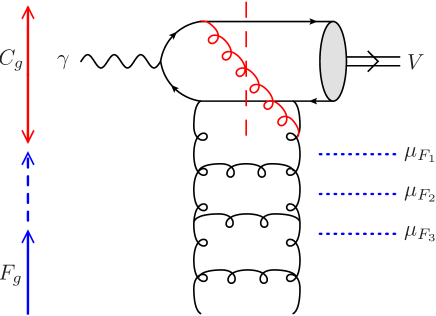
We can also explain this pictorially. As noted above, the $\mu_{F}$ dependence of the NLO correction is caused by the subtraction of the contribution generated by the evolution equation. In particular, the correction which (i) depends on $\mu_{F}$ and (ii) is enhanced by $\ln(1/\xi)$, is generated by the ladder-type diagrams shown in Fig. 2. The choice of the factorisation scale $\mu_{Fi}$ determines which part of the diagram is attributed to the evolution of the PDF and which to the hard matrix element. By choosing the value of $\mu_{F}=\mu_{0}=M_{V}/2$ we include all the ladder cells in the LO part, so that the remaining NLO matrix element will not receive any contribution from ladder-type diagrams (at small $\xi$). Note that the ladder diagrams would contribute to the NLO matrix element (from $\mu_{F}$ to $\mu_{0}$) if we were to choose a scale $\mu_{F}<\mu_{0}$. For the choice $\mu_{F}>\mu_{0}$ the NLO matrix element would contain the ladder diagrams with the negative sign in order to compensate the extra contributions (from $\mu_{0}$ to $\mu_{F}$) included in the LO part.

Since we consider an exclusive process, the mass of the final state is fixed, but the intermediate states, corresponding to the discontinuity which gives the imaginary part of the amplitude (depicted using a dotted line in Fig. 2), depend on the choice of scale. For larger values of $\mu_{F}$ the mass of the allowed intermediate states in the matrix element becomes smaller. Of course, it is impossible to absorb inside the evolution all intermediate states other than the heavy quark pair $Q{\bar{Q}}$ state which produces the $V$; for example we cannot absorb the effects of the uppermost gluon in Fig. 2 emitted by the upper heavy quark. Nevertheless, when we choose the appropriate scale $\mu_{F}=M_{V}/2$, the mass of the remaining intermediate states becomes of the order of $M_{V}$. This choice will move $\ln(1/\xi)$ contributions from the matrix element into the GPD. It will therefore provide a much more stable final result, since the remaining NLO contributions then cannot be enhanced by the large values of $\ln(1/\xi)$.

It should be emphasised that the asymptotics of the NLO amplitude is used only to determine the effective scale $\mu_{F}$. In all our further numerics we use the full expression for the complete NLO amplitude as given in [24, 32, 33].

3 Can exclusive vector meson production data be included in a global PDF fit?

In this section we present our results for the exclusive $\gamma p\to J/\psi+p$ and $\gamma p\to\Upsilon+p$ processes as functions of the factorisation scale $\mu_{f}$, and the renormalisation scale $\mu_{R}$. The cross section relies sensitively on the gluon PDF at small $x$, in a kinematic regime where it is very poorly known, as well as depending of the choice of scales. For these quasi-elastic processes we present just the dominant imaginary part of the amplitude. The real part of the coefficient functions has been calculated exactly, both via a dispersion relation [24] and by directly computing the real part of the loop integrals [32, 33], it is non-zero in the time-like region $|x|<\xi$. Therefore, to compute the real part of the amplitude directly, we need also the GPDs in this region. Unfortunately, the Shuvaev transform is not valid in the time-like region [23]. Nevertheless, the real part of the amplitude can be included via dispersive methods on the level of the amplitude. However, giving a prediction of the full cross section is not our objective here. Rather our aim is to study the stability of the perturbative predictions and to investigate whether or not we can determine optimum scales so that experimental data for these processes, and the related $pp\to p\,V\,p$ processes, can be included in global PDF (collinear) analyses to constrain the gluon PDF at low $x$, in a domain for which, at present, there are no data. For this goal it is sufficient to work with the more simple imaginary part of the amplitude.

We recall the main result of Section 2. We start from the key equation, (14), that is

$$A^{(0)}(\mu_{f})+A^{(1)}(\mu_{f})~{}=~{}C^{(0)}\otimes F(\mu_{F})+\alpha_{s}C^{(1)}_{\rm rem}(\mu_{F})\otimes F(\mu_{f})\,.$$ (16)

To obtain this result we had introduced by hand a new scale $\mu_{F}$ in the LO term and showed that the choice $\mu_{F}=m=M_{V}/2$ allowed us to resum and transfer all the enhanced large $\ln(1/\xi)$ terms from the NLO contribution to the LO term, leaving a much smaller remaining NLO contribution $\alpha_{s}C^{(1)}_{\rm rem}(\mu_{F})\otimes F(\mu_{f})$. There is still a $\mu_{f}$ scale dependence, but now this should be much weaker.

3.1 The process $\gamma p\to J/\psi+p$

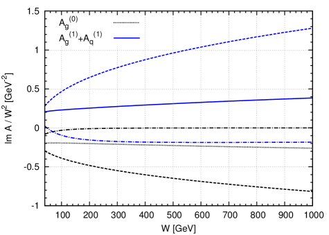
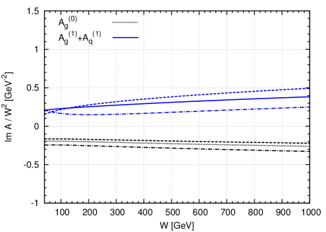
To obtain predictions for exclusive $J/\psi$ photoproduction we are working at scales close to the input GPDs used in the calculation. The results for the scale variation of the imaginary part of the amplitude are shown in the two plots of Fig. 3. In each plot we show separately the LO and NLO contributions to the amplitude. The left plot shows how these contributions change if we vary all the scales $\mu_{f}=\mu_{F}=\mu_{R}\equiv\mu$ simultaneously, taking $\mu^{2}=m^{2}/2,~{}m^{2},~{}2m^{2}$. In the right plot we fix $\mu_{F}$ at the optimum scale $\mu_{F}=m$ and vary $\mu_{f}=\mu_{R}\equiv\mu$. The result is dramatic. The transfer of the $\ln(1/\xi)$ terms from the NLO to the LO contribution has significantly reduced the $\mu_{f}$ scale dependence.

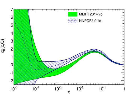
But there is another, more severe problem. The LO contribution is dominated by the NLO contribution of opposite sign. Thus the imaginary part of the quasi-elastic $\gamma p\to J/\psi+p$ amplitude changes sign when the NLO contribution is added. As it stands, this result is in contradiction with modelling the interaction as an elastic forward scattering where the imaginary part of the amplitude is positive. What is happening? The explanation is interesting. In general, the global DGLAP PDF analyses start from input forms which are completely arbitrary and, moreover, neglecting any constraints, know nothing about the structure of the evolution at low $Q^{2}$. It is then found that the gluon PDF tends to be small, or even negative, in the low $Q^{2}$, low $x$ $(10^{-4}\lower 3.01385pt\hbox{$\;\stackrel{{\scriptstyle\textstyle<}}{{\sim}}\;$}x\lower 3.01385pt\hbox{$\;\stackrel{{\scriptstyle\textstyle<}}{{\sim}}\;$}10^{-2})$ domain, see Fig. 4. Clearly due to the lack of data constraints in this domain the gluon is not reliably known.

Figure 3: Predictions of $\mathrm{Im}A/W^{2}$ for $\gamma p\rightarrow J/\psi+p$ as a function of the $\gamma p$ centre-of-mass energy $W$, produced using CTEQ6.6 partons [40] with scales $\mu\equiv\mu_{F}=\mu_{f}=\mu_{R}$ (left panel) and $\mu\equiv\mu_{f}=\mu_{R}$ with $\mu_{F}^{2}=2.4~{}\rm GeV^{2}$ (right panel). The bottom (top) set of curves corresponds to the Born (1-loop) contribution with the scale variation $\mu^{2}=1.2,2.4,4.8~{}\rm GeV^{2}$. The dot-dashed, solid and dashed lines correspond to the low, central and high values of the scale $\mu$, respectively. Note that for the left panel, the bands overlap for energies bigger than about $70~{}\rm GeV$.

Let us study the over-simplified case with an input gluon $g(x)=0$ so that at the input scale we have only quark PDFs. For $\gamma p\to J/\psi+p$ the quark contribution only appears at NLO. The imaginary part of this NLO contribution is negative with respect to the normal $(g\neq 0)$ LO term. Indeed, when calculating the NLO coefficient function we must subtract the contribution which is already generated by LO evolution. However, the subtraction is performed purely formally in order to avoid the infrared divergence and does not account for the actual value of the gluon density used to calculate the LO term. Therefore, at low scales, where the LO term is suppressed by much too small ‘unphysical’ gluon PDFs obtained from the global fits, the NLO term generated by the quark is not just a correction, but is the dominant contribution. As a consequence, the imaginary part of the quasi-elastic amplitude becomes negative (in comparison with the LO contribution) and the observed behaviour reveals a lack of stability of the perturbative series at this order. Of course, at high scales where evolution, and not the input, determine the PDFs, we obtain a sensible NLO prediction.

Figure 4: The gluon distribution at $Q^{2}=1.21~{}\rm GeV^{2}$ as determined by two recent global analyses [1, 2]. Figure produced using [42, 43].

This simple consideration demonstrates that if $\gamma p\to J/\psi+p$ and $pp\to p+J/\psi+p$ data could be included in a global fit, then they would put a strong constraint on the low $x$ input gluon distribution. It is not simply that $g(x)$ must be positive, but that actually the input gluons cannot be smaller than the density of gluons emitted by the quarks before the beginning of the evolution, when the parton virtuality $Q<Q_{0}$. If $J/\psi$ data would have been included in the collinear global parton analyses, this constraint on the low $x$ input gluon would have been automatically satisfied.

Indeed, it is seen from the second plot of Fig. 3 that after the $\ln(1/\xi)$ enhanced corrections are resummed by fixing $\mu_{F}=m$, the stability of both the LO and the NLO components of the amplitude under the scale variations are much better. From this viewpoint the $J/\psi$ data may be included in a global PDF analysis. The only problem is that the gluon density obtained in the existing PDF analyses is too small at input scales and low $x$ ($10^{-5}\lower 3.01385pt\hbox{$\;\stackrel{{\scriptstyle\textstyle<}}{{\sim}}\;$}x\lower 3.01385pt\hbox{$\;\stackrel{{\scriptstyle\textstyle<}}{{\sim}}\;$}10^{-2}$), so that we get the wrong sign of the imaginary part of the amplitude. This means that if $J/\psi$ data were included in the global PDF analyses, we must get a larger gluon density at low scales. Larger gluons in this kinematic domain will increase the LO component of the $J/\psi$ photoproduction amplitude and will provide the correct sign for the whole LO+NLO amplitude.

3.2 The processes $\gamma p\to\Upsilon+p$ and $pp\to p\Upsilon p$

Figure 5: Predictions of $\mathrm{Im}A/W^{2}$ for $\gamma p\rightarrow\Upsilon+p$ as a function of the $\gamma p$ centre-of-mass energy $W$, produced using CTEQ6.6 partons [40]. The scales are $\mu\equiv\mu_{F}=\mu_{f}=\mu_{R}$ (top left), $\mu\equiv\mu_{f}=\mu_{R}$ with $\mu_{F}^{2}=22.4~{}\rm GeV^{2}$ (top right), $\mu\equiv\mu_{f}$ with $\mu_{F}^{2}=\mu_{R}^{2}=22.4~{}\rm GeV^{2}$ (bottom left), $\mu\equiv\mu_{R}$ with $\mu_{f}^{2}=\mu_{F}^{2}=22.4~{}\rm GeV^{2}$ (bottom right). The top (bottom) set of curves corresponds to the LO (LO+NLO) contribution with the scale variation $\mu^{2}=11.9,22.4,44.7~{}\rm GeV^{2}$. The dot-dashed, solid and dashed lines correspond to the low, central and high values of the scale $\mu$, respectively. The large GPD uncertainties are not shown.

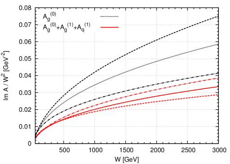
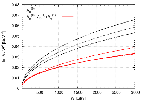
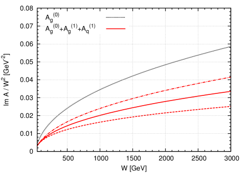
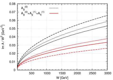
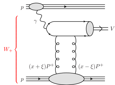
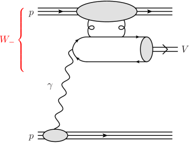
The top two plots of Fig. 5 show the results for the scale sensitivity of $\gamma p\to\Upsilon+p$, analogous to those of Fig. 3 for $\gamma p\to J/\psi+p$. Again we see that fixing the scale $\mu_{F}=M_{\Upsilon}/2$ reduces the $\mu_{f}$ scale uncertainty. The lower two plots show that part of this stability arises because the change caused by variation of $\mu_{R}$ is to some extent compensated by an ‘opposite’ change due to the variation of $\mu_{f}$. If we were to choose a non-optimal scale, say for example, $\mu^{2}_{F}=2m^{2}$, then the scale variation turns out to be about twice as large as for the optimal choice $\mu^{2}_{F}=m^{2}$. Due to the larger $\Upsilon$ mass we are now working at scales with more perturbative stability. The LO contribution is partly cancelled by the NLO term, but is not dominated by it. If we take the upper right or lower left plot of Fig. 5 then the $\mu_{f}$ scale uncertainty of the amplitude is about $\pm 15\%$ and $\pm 25\%$ respectively. As a result the data for exclusive $\Upsilon$ production can be used in global PDF analyses to probe the gluon distribution down to $x\sim 10^{-5}$, in the case of LHCb kinematics. The calculation of exclusive $pp\to p\Upsilon p$ is described in [35]. It is based on the sum of the two diagrams shown in Fig. 6. For an $\Upsilon$ produced at large rapidity $y$, the dominant contribution is from the diagram with the larger $\gamma p$ centre-of-mass energy $W_{+}$, which depends on the gluon density at $x\simeq M_{\Upsilon}~{}e^{-y}/\sqrt{s}$. The small contribution from the other diagram, with much lower energy $W_{-}$, may be estimated from the existing HERA data.

Figure 6: The two diagrams describing exclusive $\Upsilon$ production at the LHC. Diagram (a), the $W_{+}$ component, is the dominant contribution for an $\Upsilon$ produced at large rapidity $y$. Thus data for $pp\to p\Upsilon p$ allow a probe of very low $x$ values, $x\simeq M_{\Upsilon}~{}e^{-y}/\sqrt{s}$; recall that in the (dominant) imaginary part of the Born amplitude we have $x=\xi$.

If we use the central values of the presently available PDF sets obtained from global analyses, then we find cross section predictions which are about a factor of four below the HERA exclusive $\Upsilon$ data [6, 14, 15]. This indicates that future PDF global analyses with $\Upsilon$ data included will, just as for $J/\psi$ data, require a larger gluon distribution at low values of $x$. While the exclusive $\Upsilon$ process samples the PDFs at scales $Q^{2}\sim M_{\Upsilon}^{2}/4$, the larger gluon required at these $Q^{2}$ will affect the gluon densities at all values of $Q^{2}$ via the evolution.

3.3 Note on the alternative $k_{t}$-factorisation approach

The collinear DGLAP global analyses tend to result in gluon distributions with valence-like $x$ distributions at low scales, see Fig. 4. On the other hand, the approach used in the JMRT paper [35], to study exclusive vector meson production, is free from this problem. There, the ‘NLO’ prediction was not calculated as a correction from NLO Feynman diagrams in collinear factorisation, but approximated by taking the full integral over the gluon $k_{t}$ in Fig. 1(a), including an ansatz for the now $k_{t}$ dependent gluon. The convergence of this explicit $k_{t}$ integral provides effectively the ‘optimal’ value of the factorisation scale and in this way sums all $\ln(1/\xi)$ enhanced terms, accounting for a large part of the NLO corrections. It does, of course, not include corrections from diagrams which do not have a ladder structure, however, the contribution from the light quarks, Fig. 1(b), is already included in the unintegrated gluon distribution used in JMRT [35]. Clearly, then the quasi-elastic amplitude is positive definite. Let us briefly describe how our ‘NLO’ predictions for $\gamma p\to\Upsilon+p$ data were made. First the incoming gluon distribution was fitted, within this approach and using an ansatz for the gluon based on the important double-logarithmic dependence on $\ln(1/x)$ and $\ln Q^{2}$, to reproduce the $J/\psi$ data from HERA and the LHC. Then we proceeded to $\Upsilon$ production using our fitted gluon. We verified that, in the relevant kinematic domain, this gluon reproduces the NLO DGLAP evolution to good accuracy. Therefore it was not surprising that the ‘NLO’ predictions for the $\Upsilon$ cross section, as a function of $W$, agreed well with the LHCb data [18] when they became available.

4 Conclusions

Here we have been concerned about the inclusion of exclusive vector meson production data in global PDF analyses in order to probe the gluon density at small values of $x$; that is, in the $x\lower 3.01385pt\hbox{$\;\stackrel{{\scriptstyle\textstyle<}}{{\sim}}\;$}10^{-4}$ domain. Note that in this domain the input gluon PDF is freely parametrized, and is found to have a tendency to be valence-like with large uncertainties. It was hoped that the situation would be changed as data for exclusive vector meson production, $V=J/\psi$ and $\Upsilon$, which are very sensitive to the gluon at small $x$, became available at HERA and the LHC; particularly measurements of the exclusive process $pp\to p\,V\,p$ at the LHC with $V$ detected at large rapidity. Why has this not happened (so far)?

For $J/\psi$, the main problem is, at first sight, the very poor convergence of the perturbative expansion in the collinear approach. This can be seen, e.g., from Fig. 3, where the NLO contribution is comparable to the LO term and opposite in sign. However, we argued that this large NLO contribution, in comparison with that of the LO, reflects not the poor convergence, but rather that the global PDF analyses find a gluon density which is too small at low $x$ and low scales. For this reason we find a LO contribution to exclusive $J/\psi$ photoproduction amplitude which is too small. We argued that the input gluon in the collinear approach, used in the global PDF analyses, should not be parametrized freely, but should be subject to some constraints. We noted that working in the physical, $k_{t}$-factorisation type scheme would avoid these problems.

For exclusive $\Upsilon$ production the situation is much better. We found that the optimum factorisation scale is much higher, the perturbative expansion at NLO in collinear factorisation converges well, and the remaining mild scale dependence of the predictions ($\sim\pm 15\%$ on amplitude level) means that data for $pp\to p\Upsilon p$ can now be included in the global PDF fits to determine the gluon in the low $x$ regime for the first time.

It is appropriate to list the theoretical uncertainties of the present calculation. Although the leading double log terms have been resummed correctly to all orders, there still exist remaining NNLO and higher contributions, which are unknown at present. When the full NNLO amplitude is known we showed how the scale uncertainty can be further reduced. Next, we consider the accuracy of the expressions which relate GPDs to conventional PDFs, (8) and (9). These relations are based on conformal invariance and the equality of the Gegenbauer moments of GPDs to the Mellin moments of PDFs. Due to the polynominal property [21] the accuracy of this equality of the moments is ${\cal O}(\xi^{2})$, providing an ${\cal O}(\xi)$ accuracy for (8) and (9), see [23]. However, recall that the Shuvaev transform assumes the absence of the singularities in the right-half Mellin-$N$ plane for the input distribution. This assumption is physically reasonable since in the Regge approach there are no singularities in the right-half ($j>1$) plane in the space-like ($|x|>\xi$) domain where we actually work. Nevertheless, whenever possible, this assumption should be checked. One check is that the predictions for the GPD/PDF ratio obtained in this way are in a good agreement (especially for low $x$ gluons, which are the most important for exclusive $J/\psi$ or $\Upsilon$ production) with the NLO results of [44] coming from a fit to deeply virtual Compton scattering (DVCS) HERA data. Finally, the relativistic correction to the vector meson wave function, which is discussed in Section 2.2, is not expected to be significant [34].

We noted that an alternative probe of the low $x$ gluon at low scales has been considered in [29, 30]. There they study the data for charm (and beauty) production obtained in the forward direction by the LHCb Collaboration [27, 28]. Again it is found that the predictions strongly depend on the choice of factorization scale. Their prediction is lower than the data if the natural scale $\mu_{F}^{2}=m_{Q}^{2}+p_{t}^{2}$ is chosen, and it is found that a larger $\mu_{F}$ is needed to reproduce the data using the existing global PDFs. Thus our expectation of a larger gluon at low $x$ is not in contradiction with the LHCb charm (and beauty) forward data.

References

- [1] R.D. Ball et al. [NNPDF Collaboration], JHEP 1504 (2015) 040.
- [2] L.A. Harland-Lang, A.D. Martin, P. Motylinski and R.S. Thorne, Eur. Phys. J. C75 (2015) 5, 204.
- [3] S. Dulat, T.J. Hou, J. Gao, M. Guzzi, J. Huston, P. Nadolsky, J. Pumplin and C. Schmidt et al., arXiv:1506.07443 [hep-ph].
- [4] S. Aid et al. [H1 Collaboration], Nucl. Phys. B468 (1996) 3-36.
- [5] S. Aid et al. [H1 Collaboration], Nucl. Phys. B472 (1996) 3-31.
- [6] C. Adloff et al. [H1 Collaboration], Phys. Lett. B483 (2000) 23-35.
- [7] A. Aktas et al. [H1 Collaboration], Eur. Phys. J. C46 (2006) 585-603.
- [8] C. Alexa et al. [H1 Collaboration], Eur. Phys. J. C73 (2013) 2466.
- [9] M. Derrick et al. [ZEUS Collaboration], Phys. Lett. B350 (1995) 120-134.
- [10] J. Breitweg et al. [ZEUS Collaboration], Z. Phys. C75 (1997) 215-228.
- [11] J. Breitweg et al. [ZEUS Collaboration], Eur. Phys. J. C6 (1999) 603-627.
- [12] S. Chekanov et al. [ZEUS Collaboration], Eur. Phys. J. C24 (2002) 345-360.
- [13] S. Chekanov et al. [ZEUS Collaboration], Nucl. Phys. B695 (2004) 3-37.
- [14] J. Breitweg et al. [ZEUS Collaboration], Phys. Lett. B437 (1998) 432-444.
- [15] S. Chekanov et al. [ZEUS Collaboration], Phys. Lett. B680 (2009) 4-12.
- [16] R. Aaij et al. [LHCb Collaboration], J. Phys. G40 (2013) 045001.
- [17] R. Aaij et al. [LHCb Collaboration], J. Phys. G41 (2014) 055002.
- [18] R. Aaij et al. [LHCb Collaboration], arXiv:1505.08139 [hep-ex].
- [19] B. Abelev et al. [ALICE Collaboration], Phys. Rev. Lett. 133 (2014) 23, 232504.
- [20] A.J. Baltz et al., Phys. Rept. 458 (2008) 1.
- [21] X-D. Ji, J. Phys. G24 (1998) 1181.
- [22] A.G. Shuvaev, Phys. Rev. D60 (1999) 116005.
- [23] A.D. Martin, C. Nockles, M.G. Ryskin, A.G. Shuvaev and T. Teubner, Eur. Phys. J. C63 (2009) 57-67.
- [24] D.Yu. Ivanov, A. Schäfer, L. Szymanowski and G. Krasnikov, Eur. Phys. J. C34 (2004) 3, 297, Erratum ibid. C75 (2015) 2, 75, Erratum arXiv:hep-ph/0401131v3.
- [25] D.Yu. Ivanov, B. Pire, L. Szymanowski and J. Wagner, AIP Conf. Proc. 1654 (2015) 090003.
- [26] Y.L. Dokshitzer, D. Diakonov and S. Troian, Phys. Rept. 58 (1980) 269-395.
- [27] R. Aaij et al. [LHCb Collaboration], Nucl. Phys. B871 (2013) 1.
- [28] R. Aaij et al. [LHCb Collaboration], JHEP 1308 (2013) 117.
- [29] O. Zenaiev et al., Eur. Phys. J. C75 (2015) 396.
- [30] R. Gauld, J. Rojo, L. Rottoli and J. Talbert, arXiv:1506.08025 [hep-ph]
- [31] C. Nockles, Diffractive Processes and Parton Distribution Functions in the Small Regime, PhD thesis, University of Liverpool, August 2009 (unpublished).
- [32] S.P. Jones, A Study of Exclusive Processes to NLO and Small- PDFs from LHC Data, PhD thesis, University of Liverpool, September 2014 (unpublished).
- [33] J. Gracey, S.P. Jones and T. Teubner, in preparation.
- [34] P. Hoodbhoy, Phys. Rev. D56 (1997) 388.
- [35] S.P. Jones, A.D. Martin, M.G. Ryskin and T. Teubner, JHEP 1311 (2013) 085.
- [36] J. Bartels and M. Loewe, Z. Phys. C12 (1982) 263.
- [37] M.A. Kimber, A.D. Martin and M.G. Ryskin, Phys. Rev. D63 (2001) 114027.
- [38] A.D. Martin, M.G. Ryskin and G. Watt, Eur. Phys. J. C66 (2010) 163.
- [39] E.G. de Oliveira, A.D. Martin and M.G. Ryskin, Eur. Phys. J. C72 (2012) 2069.
- [40] Q. Cao, J. Huston, H. Lai, P.M. Nadolsky, J. Pumplin, W. Tung, D. Stump and C.-P. Yuan, Phys. Rev. D78 (2008) 013004.
- [41] A.D. Martin, C. Nockles, M.G. Ryskin and T. Teubner, Phys. Lett. B662 (2008) 252-258.
- [42] V. Bertone, S. Carrazza and J. Rojo, Comput. Phys. Commun. 185 (2014) 1647-1668, arXiv:1310.1394 [hep-ph].
- [43] S. Carrazza, A. Ferrara, D. Palazzo and J. Rojo, J. Phys. G42 (2015) 057001, arXiv:1410.5456 [hep-ph].
- [44] K. Kumericki and D. Muller, Nucl. Phys. B841 (2010) 1.