Applying Exclusion Likelihoods from LHC Searches to Extended Higgs Sectors
Abstract
LHC searches for non-standard Higgs bosons decaying into tau lepton pairs constitute a sensitive experimental probe for physics beyond the Standard Model (BSM), such as Supersymmetry (SUSY). Recently, the limits obtained from these searches have been presented by the CMS collaboration in a nearly model-independent fashion — as a narrow resonance model — based on the full dataset. In addition to publishing a exclusion limit, the full likelihood information for the narrow resonance model has been released. This provides valuable information that can be incorporated into global BSM fits. We present a simple algorithm that maps an arbitrary model with multiple neutral Higgs bosons onto the narrow resonance model and derives the corresponding value for the exclusion likelihood from the CMS search. This procedure has been implemented into the public computer code HiggsBounds (version 4.2.0 and higher). We validate our implementation by cross-checking against the official CMS exclusion contours in three Higgs benchmark scenarios in the Minimal Supersymmetric Standard Model (MSSM), and find very good agreement. Going beyond validation, we discuss the combined constraints of the search and the rate measurements of the SM-like Higgs at in a recently proposed MSSM benchmark scenario, where the lightest Higgs boson obtains SM-like couplings independently of the decoupling of the heavier Higgs states. Technical details for how to access the likelihood information within HiggsBounds are given in the appendix. The program is available at http://higgsbounds.hepforge.org.
I Introduction
The search for Higgs bosons Englert:1964et ; *Higgs:1964ia; *Higgs:1964pj; *Guralnik:1964eu; *Higgs:1966ev; *Kibble:1967sv continues to be a cornerstone of the physics program at the Large Hadron Collider (LHC). After the discovery of a Higgs boson by ATLAS Aad:2012tfa and CMS Chatrchyan:2012ufa it is crucial to find out whether the detected particle is part of a Higgs sector that contains several physical states. Higgs sectors of this kind are predicted in many theories of physics beyond the Standard Model (SM). For the understanding of the mechanism of electroweak symmetry breaking two complementary experimental endeavors are important: On the one hand the precise determination of the properties of the Higgs signal detected at around , and on the other hand the search for additional Higgs bosons. Both are crucial in the quest to identify the underlying physics. The existing limits from the Higgs searches at LEP, the Tevatron and the LHC already put very important constraints on the parameter spaces of different models that provide a Higgs-like state compatible with the detected signal. More data on both the detected signal and on searches for additional Higgs bosons will further enhance the sensitivity for discriminating possible scenarios of new physics from the SM and from each other.
In order to facilitate the available experimental information from the Higgs searches at LEP, the Tevatron and the LHC, expressed in terms of relatively model-independent cross-section limits for testing a wide variety of theoretical models, the program HiggsBounds Bechtle:2008jh ; Bechtle:2011sb ; Bechtle:2013gu ; Bechtle:2013wla has been developed. Experimental information on the Higgs signal detected at a mass value of around is utilized in the sister program HiggsSignals Bechtle:2013xfa for testing the theoretical predictions from any kind of Higgs sector. The experimental information on the detected signal incorporated in HiggsSignals is turned into a likelihood, which is suitable for the inclusion into global fits (see, e.g., Refs. deVries:2015hva ; Bechtle:2012jw ; Bechtle:2012zk ; Bechtle:2013mda ; Bechtle:2014yna ; Bechtle:2014ewa ), where in addition many other observables are taken into account. In contrast, exclusion limits have traditionally been presented in terms of limits, which a priori only provide the information whether a particular parameter point is excluded or not at the by the considered search channel. In a global fit, where the predictions of a model are confronted with a large number of observables, it would usually be too restrictive to disregard a certain parameter point just because it falls outside of the region of a single search channel. In fact, testing a large variety of observables one would expect that the measured values of some observables lie outside of the respective regions for purely statistical reasons. It would therefore be very desirable if also negative experimental outcomes from Higgs searches were provided in terms of the likelihood information in the relevant parameters, instead of a simple binary rejection or acceptance at a certain confidence level (C.L.). Up to now, likelihood information was available in HiggsBounds only for the results from the LEP Higgs searches Bechtle:2013wla , while for all search channels at the Tevatron and LHC only limits have been accessible. We report here on significant progress in this direction for the LHC Higgs boson search in the final state, which plays a central role in the search for additional Higgs bosons.
Many models that can accommodate a SM-like Higgs boson at , such as the Minimal Supersymmetric Standard Model (MSSM) or the various types of Two-Higgs-Doublet Models (2HDM), predict additional Higgs bosons that decay predominantly into SM fermions. Therefore, LHC searches for new neutral Higgs bosons decaying to play a crucial role. In particular within the MSSM, these searches lead to large excluded regions in the parameter space. The highest experimental sensitivity occurs for smaller values of the -odd Higgs boson mass, , and larger values of , the ratio of the two vacuum expectation values Khachatryan:2014wca ; Aad:2014vgg .
One complication that arises for this search channel is the fact that two different production modes, gluon fusion and quark associated production, can both be important. Their individual contributions to the signal rate can vary strongly over the parameter space. Since the acceptances of these two channels can also be very different, a two-dimensional cross section interpretation for the final state is desirable as a basis for (close to) model-independent exclusion limits. Recently, the CMS collaboration has published the likelihood information for their Higgs boson search in the final state Khachatryan:2014wca . The likelihood is given as a function of the two relevant Higgs production channels, gluon fusion and quark associated production, for various mass values of the narrow resonance assumed for the signal model.
In this paper we investigate the application of this new experimental information for testing the theoretical predictions of extended Higgs sectors and its incorporation in global fits. We develop a simple algorithm that maps an arbitrary model with in general several neutral Higgs bosons onto the narrow resonance model. In this way the corresponding value of the exclusion likelihood from the CMS search for the tested model can be determined. We furthermore describe the inclusion of this likelihood information into the publicly available Fortran code HiggsBounds Bechtle:2008jh ; Bechtle:2011sb ; Bechtle:2013gu ; Bechtle:2013wla . For nearly any model under consideration, HiggsBounds provides an evaluation of the exclusion likelihood for a model parameter point based on the information from Ref. Khachatryan:2014wca . While the new likelihood information goes well beyond the standard test whether a particular parameter point is excluded at the , the likelihood information can also be employed to run HiggsBounds in this “standard” mode. In this case, HiggsBounds determines the parameter region that is excluded at the based on all available searches, including the new result from CMS. The new version of HiggsBounds can be used together with its sister program HiggsSignals Bechtle:2013xfa in order to take into account both the information from search limits and from the detected signal for a comprehensive test of Higgs phenomenology. Both codes are available at:
The paper is organized as follows. In Section II we briefly summarize the experimental results that are used as input for our investigations. Details of the employed algorithm and the implementation of the exclusion likelihood of Ref. Khachatryan:2014wca into HiggsBounds are given in Section III. The validation in various MSSM Higgs benchmark scenarios is discussed in Section IV. As an application, in Section V we investigate the constraints on a certain benchmark scenario in the MSSM that are obtained from using the new exclusion likelihood in combination with the information on the detected signal incorporated in HiggsSignals. We conclude in Section VI. Finally, all relevant information needed to run HiggsBounds to obtain the likelihood information for the Higgs search channel for any parameter point under investigation are contained in an Appendix.
II Experimental results
This section briefly summarizes the experimental results from the CMS non-standard Higgs search in the final state Khachatryan:2014wca , that we have used as starting point for our investigation and that we have implemented in HiggsBounds. The search analysis of CMS is carried out in two separate selection categories: One requiring the presence of at least one -tagged jet, and one without the presence of a -tag. The former category is enriched by the production of a Higgs boson, denoted generically by , in association with two quarks, , while the latter is dominated by the gluon fusion process, . Hence, the search features sensitivity to the two different production modes separately, which enables the presentation of the search results in terms of individual signal strengths in both production modes for all tested Higgs boson masses. Separate information on the two production modes is an indispensable ingredient for enabling the presentation of (close to) model-independent exclusion limits or measurements, in case of a discovery.
The data is further classified in categories defined by the two lepton decay modes: , , , and , where denotes a hadronically decaying lepton. Using a maximum likelihood technique, an estimator for the true invariant mass, , is reconstructed from the momenta of the visible decay products and the missing transverse energy in the event. The uncertainty of the reconstruction is estimated to be around when averaged over all decay modes Khachatryan:2014wca .
The resulting spectrum in all categories (-tag and decay) separately is then subject to a profile likelihood analysis CMS-NOTE-2011-005 , where the background parametrization, obtained from control region data and Monte Carlo simulation, and the signal shape parametrization are fitted simultaneously to the reconstructed mass spectrum. The fit is performed individually for test masses between and , and the results are interpolated between the test masses.
CMS interprets the results both in a nearly model-independent way111The presentation of the search results in terms of a limit on the inclusive total cross section times branching ratio inevitably involves a slight model dependence from the extrapolation to the inclusive quantity. In other words, the expectation of the kinematic distributions of the signal and/or background is model dependent. for a single narrow resonance , and, in a model-specific context, in the MSSM, where three neutral Higgs bosons , and potentially comprise the signal. The latter interpretation performs a likelihood ratio hypothesis test for the two hypotheses of a single SM-like Higgs boson at with exact SM properties and, alternatively, for the signal consisting of all three neutral Higgs bosons of the MSSM. In the latter case, the distributions of the decays are combined before the calculation of the likelihood. Note that, whereas the model-specific limits for the MSSM are based on the full integrated luminosity of the combined dataset, the results for the single narrow resonance model are obtained from only the dataset.
Since HiggsBounds is designed to test any extended Higgs sector, with any coupling properties of the Higgs candidate (if the model under consideration provides such a candidate; obviously the phenomenological interest in other models is rather limited) and any masses and properties of the remaining Higgs spectrum, the nearly model-independent single resonance results are chosen for the implementation in HiggsBounds. On the one hand, this is the only possibility unless one is willing to adopt further model-dependent assumptions. On the other hand, it will in general yield weaker, i.e. more conservative, limits than a dedicated analysis taking into account the full structure of the considered model. For example, in the MSSM this will yield a conservative limit whenever either , or, more generally, whenever the model predicts that more than one Higgs boson have a non-negligible signal yield and contribute in different regions in . Since the likelihood is constructed for single resonances, such a case cannot be properly reconstructed from the likelihood. However, if e.g. the heavy MSSM Higgs bosons and contribute at the same point in , their signal rates can be added before interpreting the likelihood. In this case the implementation is not necessarily conservative. A detailed study on the applicability of these limits to the MSSM benchmarks is presented in Section IV.
The profile likelihood analysis follows the standard implementation: The test statistics is given by
| (1) |
Here is the number of measured events, and the number of expected background and signal events for a given resonance mass hypothesis , the signal strength modifier, and are the nuisance parameters decribing the systematic uncertainties. maximizes the likelihood in the numerator given a certain value of , whereas the likelihood reaches its global maximum at and , which is given in the denominator. The constraint is employed to not penalize the model for a possible excess of the data over the signal plus background prediction. It should be noted that the signal yield contains two independent components, corresponding to the two production modes and . Thus, and are two-component vectors.
Using toy Monte Carlo techniques or asymptotic expressions for large statistics, the expected probability distributions can be constructed for the test statistics given above. In the model-independent analysis used here, the hypothesis either consists of for the case of the presence of a single narrow resonance with a given mass and signal yield , and of for the background. Using these hypothesis definitions and the observed value of the likelihood ratio, , given by Eq. (1) with given by the actual observed number of events, , the likelihood ratio technique can be used to define the as
| (2) |
In a stand-alone search, the criterion is then used to exclude the presence of a signal at confidence level (C.L.). For the expected limit, the observed data in the calculation of is replaced by the median of the background-only expectation for . A model-independent limit, e.g. at the , can then be derived by varying until . The value at which this happens then represents the signal strength modifier which is just allowed at the .
For any given model, HiggsBounds reconstructs the predicted signal yield from the theoretical input provided by the user, and obtains the corresponding value of the test statistics (or simply denoted ) from the CMS likelihood data. The details of this procedure will be described in the following section. Note that HiggsBounds directly employs the expectation and observation of the test statistics, and , respectively, as the provided CMS data does not allow for a full reconstruction of the value. Nevertheless, in the limit of large numbers, the test statistics can be approximated by a chi-squared differences function above minimum, , as
| (3) | ||||
| (4) |
Thus, for example, we approximately obtain the two-dimensional limit at the and when the test statistics takes the values and , respectively.
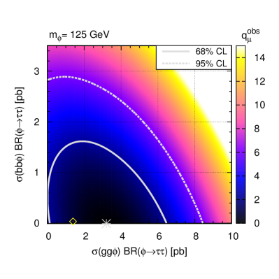
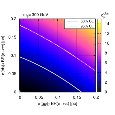
As an example, we show the observed likelihood distribution, , for test masses of and in Fig. 1. We also indicate the approximated and limits by contour lines. It should be kept in mind that these contours are only for illustrational purposes. In HiggsBounds the full likelihood information is used, and the specific limit at a certain C.L. can be easily obtained from this information.
The implementation of the likelihood for the CMS search differs in two significant ways from the implementation of the LEP Higgs search in HiggsBounds, which is already available since version 2.0.0 Bechtle:2011sb . In the LEP implementation, each Higgs search channel, comprised of one production mode and one Higgs boson decay mode, is treated separately, thus no combination of production modes is applied or possible for the user. In addition, in the LEP implementation the is estimated from the value in each channel at the given signal strength prediction using Gaussian approximations. In contrast, for the CMS search the exact values of the test statistics as presented by CMS are used and properly combined for both production modes.
III Likelihood reconstruction for extended Higgs sectors
For the construction of the exclusion likelihood from the search, we make use of the following quantities: For each neutral Higgs boson, (), in a model with neutral Higgs bosons, we have a prediction of the mass, (where the relevant range is currently ), the gluon fusion production cross section, , the cross section for production in association with quarks, , and the branching fraction .
The main algorithm for the likelihood reconstruction proceeds as follows:
-
1.
Signal rates of multiple Higgs bosons that cannot be resolved by the experimental analysis are added. We thus combine the signal predictions for two Higgs boson and , if
(5) Each Higgs boson can appear in different such combinations. For each combination, also called Higgs cluster and labeled with capital characters in the following, we evaluate the physical quantities as follows: We assume that the total rates are given by the incoherent sum of the signal rates of the individual Higgs bosons in the cluster,
(6) (7) The cluster mass, , is determined by a signal strengths weighted mass average
(8) The sums in Eqs. (6)–(8) run over all Higgs bosons combined in the cluster. In case there is no that fulfills Eq. (5) for a given , the cluster is formed solely by the Higgs boson . It should be noted that taking the incoherent sum of the contributions of the different Higgs bosons involves an approximation. While it is exact in the case of two different eigenstates, e.g. and in the MSSM, in general interference contributions can be important Fuchs:2014ola ; Fuchs:2014zra . An extension of HiggsBounds that enables the implementation of interference effects of nearby resonances in a generalized narrow-width approximation is currently under development, see also Ref. ElinaPhD .
-
2.
In the second step, the expected and observed likelihood values, and , respectively, for each Higgs cluster are evaluated from the experimental likelihood data grid. The likelihood is first evaluated for the rate values and , obtained through Eqs. (6)–(7), in the mass-neighboring data slices, i.e. at the nearest grid mass values below and above , denoted by and , respectively. The likelihood value at the predicted cluster mass is then obtained through linear interpolation:
(9) Here denote the values of the test statistics obtained at the neighboring grid above or below the predicted mass (we omitted the subscript ‘model’ for simplicity in Eq. (9)). These are obtained, in each case, through bilinear interpolation within the two-dimensional likelihood planes of the provided CMS data.
-
3.
The steps 1. and 2. are repeated until all neutral Higgs bosons have been evaluated as part of at least one Higgs cluster.
-
4.
Once all likelihoods have been evaluated, the most sensitive analysis application is determined from the resulting expected likelihood, , i.e. the cluster is selected for which is maximal. The observed exclusion likelihood, , is then used only for this cluster, and provides the final result.
Following this algorithm, the full likelihood from the CMS analysis for both the expected and observed exclusion can be directly obtained within HiggsBounds for any tested model. This is carried out via Fortran subroutines. For a technical documentation see Appendix User guide: How to obtain the exclusion likelihood with HiggsBounds.
The use of this likelihood information is complementary to the other type of information contained in a full HiggsBounds application, which considers exclusion limits from many other Higgs searches from the LEP, Tevatron and LHC experiments. As an alternative to using the full likelihood, we therefore also provide the option to reconstruct a limit at C.L. and use this in the “standard” HiggsBounds operation. For clarity, we now repeat some elements of how this works Bechtle:2013wla : In the statistical procedure, HiggsBounds first determines the most sensitive analysis to the model by picking the analysis application, for which the ratio between the model-predicted signal rate, , over the expected upper limit on the signal rate, ,
| (10) |
is maximized. After the most sensitive analysis has been determined, the model prediction is confronted with the observed exclusion limit of this particular analysis, . The model is considered to be excluded at the , if
| (11) |
For the CMS analysis described above, and are a priori not known and need to be determined from the implemented likelihood distribution. In a numerical procedure, we therefore scale the model-predicted and rates with a universal factor until the obtained expected/observed likelihood values are equal to , corresponding to the two-dimensional interval.222Technically, allowing for finite numerical precision we check for equality within . The so-obtained scale factors, , are then identified with the expected/observed upper limits on the signal rate, respectively, which enter Eqs. (10) and (11). In this way, the likelihood-based results from the CMS analysis can be incorporated in the standard HiggsBounds run.
IV Validation
Besides the nearly model-independent limits, CMS has also presented model-specific interpretations of their search results. This has been done for the MSSM, employing the benchmark scenarios proposed in Ref. Carena:2013qia (see also Ref. Heinemeyer:2013tqa ). Here, we validate our likelihood implementation in HiggsBounds against the CMS results for three of these scenarios: The , the light stop and the low- scenarios (see Ref. Carena:2013qia for details). The comparison of the reconstructed exclusion line with the official CMS result provides a non-trivial test of our implementation: Firstly, it checks whether the exclusion likelihood agrees over a wide range of different compositions of the gluon fusion and quark associated Higgs production rates obtained in the MSSM parameter space, which are mapped onto the two-dimensional likelihood grids (for fixed Higgs mass) in our reconstruction. Secondly, it tests whether our simple criterion of combining signal rates of Higgs bosons which have similar masses (overlapping within ) is a reasonable approximation. Thirdly, the validation also tests whether the results obtained from the statistical hypothesis test of a single narrow resonance model can be mapped reasonably well onto the full neutral Higgs spectrum of the MSSM (and beyond).
Some deviations can be expected at the transition between regimes with different contributing Higgs combinations. As explained above, the implementation in HiggsBounds is based on the CMS results for the single narrow resonance interpretation, and the contributions of different Higgs bosons of a considered model can only be combined if their mass differences are such that they would appear as a single resonance in the CMS search. In contrast, in the dedicated CMS analyses carried out in specific MSSM benchmark scenarios it was possible to properly combine the contributions from different Higgs bosons at any given mass constellation since these have been simulated and tested with their particular masses at every parameter point. Therefore, the dedicated CMS analysis is expected to have a higher sensitivity than the HiggsBounds implementation if multiple Higgs bosons with different masses each give a non-negligible contribution to the signal yield. Furthermore, due to the simple criterion used in HiggsBounds for including/excluding the contributions of additional Higgs bosons, the considered rates in HiggsBounds may change quite abruptly in a transition region, where the selection of the tested Higgs boson combination changes. The single resonance approximation is expected to work best when the signal can be described as a single resonance formed by one or several Higgs bosons, while contributions of other Higgs bosons besides those associated with the resonance are negligible.
For predictions in the MSSM benchmark scenarios we employ the grids of Higgs production cross sections and branching fractions for the MSSM benchmark scenarios provided by the LHC Higgs Cross Section Working Group (LHCHXSWG) LHCHXSWG_MSSM .333The LHCHXSWG cross section and branching fraction grids for the MSSM benchmark scenarios are based on the following set of tools and calculations, that we list here for completeness: HIGLU Spira:1995mt , SusHi Harlander:2012pb , FeynHiggs Heinemeyer:1998yj ; Heinemeyer:1998np ; Degrassi:2002fi ; Frank:2006yh ; Hahn:2009zz ; Hahn:2013ria , ggH@NNLO Harlander:2002wh , HDECAY Djouadi:1997yw ; Djouadi:2006bz , Prophecy4f Bredenstein:2006rh ; Bredenstein:2006ha , bbh@NNLO(5FS) Harlander:2003ai , bbh@NLO (4FS) Dittmaier:2003ej ; Dawson:2003kb , ggH NLO massive Spira:1995rr , ggH NNLO for scalar Higgs Anastasiou:2002yz ; Ravindran:2003um , ggH NNLO for pseudoscalar Higgs Harlander:2002vv ; Anastasiou:2002wq , EW corrections from light fermions Aglietti:2004nj ; Bonciani:2010ms , (N)NLO (S)QCD corrections for Harlander:2004tp ; Harlander:2005rq ; Degrassi:2010eu ; Degrassi:2011vq ; Degrassi:2012vt . For the production process we employ Santander-matching of the - and -flavor scheme (FS) cross sections Harlander:2011aa .
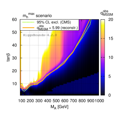
The results for the scenario in the plane are shown in Fig. 2.444Here, and in the following figures, we show as HiggsBounds result only the constraints obtained from the CMS analysis and not from the full HiggsBounds application, where all currently implemented Higgs searches from LEP, the Tevatron and the LHC are taken into account. In Fig. 2(a) we show the distribution of the observed exclusion likelihood, (in color), as obtained from HiggsBounds. The corresponding exclusion limit (orange, solid contour), which fulfills , is shown together with the CMS result obtained from a dedicated analysis in this benchmark scenario Khachatryan:2014wca (green, dashed contour). As mentioned in Section II, the latter is based on the full combined dataset, whereas the exclusion information implemented in HiggsBounds is only based on the dataset. However, this fact is expected to lead to only minor differences in the excluded parameter regions. As can be seen, there is very good agreement between the exclusion limit reconstructed with HiggsBounds and the CMS result. Small deviations can be observed in the low region, , where all three neutral MSSM Higgs bosons contribute substantially to the signal yield. Here, the result reconstructed with HiggsBounds excludes a slightly smaller area of parameter space. The HiggsBounds result can thus be regarded as a conservative estimate of the actual exclusion limit.
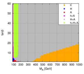
In Fig. 2(b) we display, for every parameter point in the plane, the Higgs boson or combination of Higgs bosons (cluster) that has been selected to obtain the observed exclusion likelihood by the algorithm described in Section III. It can be seen that all three neutral Higgs bosons are combined in most of the parameter region with and , whereas at larger values only the two heavier Higgs bosons, and , which are nearly mass degenerate, are combined to yield the most sensitive constraint. At low and large values, however, the combined signal rate of the heavier Higgs bosons becomes so small that it is instead the light Higgs boson, with mass around , that is selected to give the observed exclusion likelihood. This is because its expected exclusion likelihood is larger than that obtained for . The observed exclusion likelihood obtained for the light Higgs boson with mass around is non-zero because the best-fit point in the two-dimensional cross section grid at is not identical with the SM prediction, cf. Fig. 1(a). This leads to the small, but non-zero values that are visible in Fig. 2(a) at large and small .
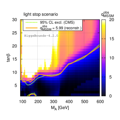
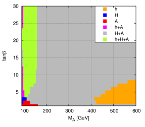
Next we look at the light stop benchmark scenario, for which the cross section predictions and their associated theoretical uncertainties have been discussed in detail in Ref. Bagnaschi:2014zla . This scenario features a relatively low SUSY particle mass scale, , and large stop mixing, , leading to a lightest stop with a mass of . This leads to a reduction of the gluon fusion cross section of the light Higgs by around with respect to the SM prediction Carena:2013qia . The results of applying our exclusion likelihood implementation in this scenario are shown in Fig. 3 (with colors similar to Fig. 2). The agreement between the exclusion contour obtained with HiggsBounds and the CMS result obtained from a dedicated analysis in this benchmark scenario Khachatryan:2014wca , as displayed in Fig. 3(a), is very good for pseudoscalar Higgs masses . Similarly as in the scenario the reconstructed exclusion limit obtained from HiggsBounds is slightly weaker for lower values than the CMS result from the analysis of the benchmark scenarios. As one can see in Fig. 3(b), the reconstructed likelihood in the low- region obtained from HiggsBounds is mainly based on a combination of the and signals, while in most part of this parameter region the light Higgs boson at GeV is not covered by the mass overlap criterion used in HiggsBounds. In contrast, in the dedicated CMS analysis in this scenario also the contribution from the light Higgs boson is properly combined with the contributions from the other neutral Higgs bosons. The latter analysis therefore has a slightly higher sensitivity in this region, which means that the exclusion bound that we find here is slightly conservative compared to the dedicated CMS result. In addition to the excluded parameter region at values of , the light stop scenario features an additional small excluded area at lower values, namely , and . The exclusion contour evaluated with HiggsBounds matches very well with the CMS result also in this region, where gluon fusion is the dominant production mode.
Finally, we test our implementation against the results obtained in the low- scenario, where the heavy -even Higgs boson is interpreted as the discovered SM-like Higgs boson at around and the light -even Higgs is largely decoupled from the SM gauge bosons Heinemeyer:2011aa . Unlike the other benchmark scenarios, which use as a free parameter, this scenario is defined as a two-dimensional parameter plane in and the Higgsino mixing parameter . The mass of the pseudoscalar Higgs, , is fixed to , which leads to a lightest Higgs mass that varies mostly between and , but reaching even lower values at very low and very high . Since in the MSSM a low value of implies also a light charged Higgs boson, this scenario served in particular as a benchmark for the LHC searches for charged Higgs bosons in top quark decays. In fact, the parameter space for this scenario in the MSSM is meanwhile essentially excluded TheATLAScollaboration:2013wia ; Aad:2014kga ; CMS:2014cdp (see also Ref. Stefaniak:2014roa ). Nevertheless this benchmark scenario is still very useful for our validation since all three neutral Higgs bosons have similar masses and thus contribute non-trivially to the analysis.
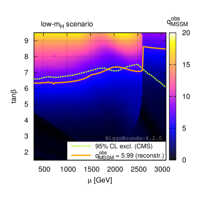
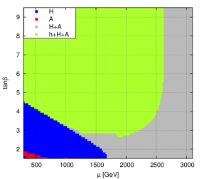
The comparison of the exclusion limits that have been reconstructed with HiggsBounds with the CMS results is shown in Fig. 4. It can be observed in Fig. 4(a) that there is rather good agreement between the exclusion limit obtained with HiggsBounds and the CMS result for values up to . At this value of (depending on ) the reconstructed exclusion limit develops an “edge”, and for higher values the reconstructed exclusion limit is significantly weaker than the one of the CMS result. The reason for this behavior is that at large the light Higgs mass becomes smaller than and is hence not combined with the heavier Higgs bosons and in HiggsBounds. This can be seen in Fig. 4(b). In this parameter region, the tested signal rate is therefore significantly smaller than in the case of a full combination of , and , and the resulting exclusion limit is accordingly weaker. In contrast, in the CMS analysis the signal yield of the light Higgs has been properly taken into account even for very low mass values, and the possibly decreasing signal efficiency is partially compensated by the increasing production cross section, leading to the significantly stronger exclusion at high values obtained by CMS.555A better agreement in the large parameter region could be obtained by increasing the mass overlap value of in the criterion for forming Higgs boson combinations to a sufficiently high value. However, firstly, there is no strong physics motivation to choose a value well beyond the quoted mass resolution of of the experimental analysis. Secondly, values larger than might lead to too aggressive exclusions in some scenarios. We therefore stick to the value of as the default setting.
In almost all the remaining parameter space, all three Higgs bosons are combined by HiggsBounds, as can be seen in Fig. 4(b), and the reconstructed exclusion contour resembles the CMS result for values below . The slight deviations observed could result from mass-dependent selection efficiencies for the and signal yields, which cannot be accounted for in the HiggsBounds implementation since this information is not publicly available. Overall, even for this rather extreme scenario in the MSSM we find that the exclusion likelihood reconstructed with HiggsBounds approximates the results of a dedicated analysis reasonably well for large parts of the parameter space.
V Example application: “Alignment without decoupling”
We now go beyond the validation with official CMS results and illustrate the usefulness of our exclusion likelihood implementation for another MSSM scenario. We consider here a scenario where the couplings of the light -even Higgs boson become SM-like for a certain range of values, independently of the masses of the remaining Higgs spectrum. The existence of this so-called alignment limit was first pointed out in Ref. Gunion:2002zf for the 2HDM. After the Higgs discovery this possibility has gained attention through a series of papers Craig:2013hca ; Asner:2013psa ; Carena:2013ooa ; Haber:2013mia ; Carena:2014nza , see also the “-phobic” benchmark scenario in Ref. Carena:2013qia . In the MSSM the alignment limit can be realized independently of the decoupling of the heavier Higgs states through a cancellation between tree-level and higher-order contributions in the Higgs sector. This cancellation can occur at relatively large values of and , with being the stop mass scale. In the approximation , and taking into account for simplicity only the dominant corrections at one loop, the alignment condition reads Carena:2014nza
| (12) |
Here, and are the boson and top quark mass, respectively. denotes the light -even Higgs boson mass in the above approximation, and . is the trilinear soft-breaking term in the stop sector.
Solutions of Eq. (12) with exist if . Typically, in order to achieve the correct Higgs mass for not too large values of the stop masses, the stop mixing is chosen in the region where the prediction for is maximized, i.e. (at one-loop). Therefore, for (), the alignment condition has viable solutions for values of that are slightly above (below) the value where the prediction for is maximized. By increasing it is possible to lower the value at which alignment occurs. An MSSM benchmark scenario of this kind for BSM Higgs searches at the LHC has recently been proposed in Ref. Carena:2014nza .
Here, we investigate the benchmark scenario proposed in Ref. Carena:2014nza , which is essentially a modification of the scenario Carena:2013qia to allow for alignment independent of decoupling. This so-called scenario is defined by the parameter values (in the on-shell scheme)
| (13) |
In contrast to the benchmark scenarios of Ref. Carena:2013qia , the parameters and are adjustable parameters in the scenario. For convenience, the slepton, sbottom and first and second generation squark soft-breaking mass parameters are set to , however, these can easily be adjusted to higher values in order to avoid constraints from SUSY searches at the LHC as their influence on the Higgs phenomenology is negligible here. We follow the suggestion to set to per default and, if necessary, increase this value until a light Higgs mass of is obtained. In practice, this is only relevant at very low values of in the benchmark scenario defined by Eq. (13). The parameter is then adjusted according to a chosen ratio . We focus here on the choice , implying rather large values of , where alignment independent of decoupling occurs at .
The MSSM predictions are obtained using the public computer codes FeynHiggs-2.10.2 Heinemeyer:1998yj ; Heinemeyer:1998np ; Degrassi:2002fi ; Frank:2006yh ; Hahn:2013ria for the Higgs masses, couplings and branching fractions, and SusHi-1.4.1 Harlander:2012pb for the gluon fusion and quark associated production cross sections of the three neutral Higgs bosons.
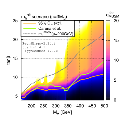
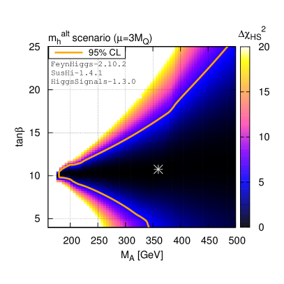
The numerical results for this benchmark scenario are displayed in Fig. 5. The observed exclusion likelihood from the CMS search as obtained from HiggsBounds is shown in color in Fig. 5(a), and the orange contour indicates the resulting observed exclusion line. For comparison, the green contour shows the exclusion line obtained in Ref. Carena:2014nza using results from the same CMS analysis, however, following a more simplistic approach.666The limit in Ref. Carena:2014nza has been obtained by “reverse-engineering” an inclusive limit from the CMS results for the scenario with Carena:2013qia , and applying this cross section limit to the given alignment benchmark scenario. In particular, this approximation does not take into account the sensitivity of the limit on the individual contributions from the gluon fusion and quark associated Higgs production processes. As can be seen from the figure, the more advanced implementation of the observed exclusion likelihood in HiggsBounds leads to a somewhat stronger exclusion limit over most of the parameter space. The relative behavior seems to be different in the threshold region, , where in particular the cross section is enhanced. However, the approximations made in Ref. Carena:2014nza appear to be least reliable in this region. The gray dotted line shows the exclusion limit obtained by CMS for the scenario. As discussed in Ref. Carena:2013qia , the excluded regions in the benchmark scenarios are significantly affected if decay modes of the heavy Higgs bosons and into SUSY particles are kinematically open and unsuppressed. The presence of such decay modes leads to a sizable reduction of the branching fractions and therefore to a smaller excluded region. In the alignment scenario is very large, leading to a negligible Higgsino component in the light neutralinos and chargino. The branching fractions for the Higgs decays to neutralinos and charginos are therefore essentially absent. In addition, the heavy Higgs decays to gauge bosons, and , are also suppressed, as the responsible coupling vanishes in the alignment limit. As a result, the branching fraction is significantly higher in the alignment scenario than in the scenario, which leads to a much larger excluded region in the alignment scenario, see also the discussion in Ref. Carena:2014nza .
In order to illustrate the complementarity between the constraints from the CMS search and the constraints obtained from the signal rate measurements of the discovered Higgs boson, we show in Fig. 5(b) the likelihood distribution, , obtained from a test of the light Higgs boson signal rates against a combination of the latest rate measurements from the LHC Aad:2014eha ; Aad:2014eva ; ATLAS:2014aga ; Aad:2015vsa ; Aad:2014xzb ; Khachatryan:2014ira ; Chatrchyan:2013mxa ; Chatrchyan:2013iaa ; Chatrchyan:2014vua and the Tevatron Aaltonen:2013ipa ; Abazov:2013gmz , using the public computer code HiggsSignals-1.3.0 Bechtle:2013xfa (see also Refs. Bechtle:2014ewa ; Stal:2013hwa ). The preferred region lies within the orange contours in Fig. 5(b). It is given by the difference with respect to the minimal value (located in the alignment region and indicated as gray asterisk in Fig. 5(b)), . It can be seen that the distribution becomes independent of at around , indicating that the couplings of the light Higgs become SM-like independently of the decoupling of the heavier Higgs states.
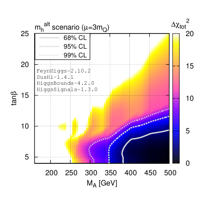
Since we now have the exclusion likelihood from the CMS search available, we can perform a statistical combination with the constraints from the Higgs rate measurements by constructing the global function . The resulting distribution777Again, is the difference with respect to the minimal value (obtained at , , i.e. in the lower right corner of Fig. 6), now based on the global likelihood . is shown in Fig. 6. The constraints from the searches at the LHC are highly complementary to the rate measurements, since they are particularly sensitive at higher values of where the production process is enhanced. In the scenario with , the combination of both constraints yields a lower limit of at the Thus, alignment of the light Higgs boson occurring without the simultaneous decoupling of the heavier Higgs states is ruled out for this scenario. The alignment without decoupling limit can be pushed to lower values of in this scenario, where the constraints from the searches are less significant, only by choosing even more extreme values of , which potentially leads to problems with vacuum stability Blinov:2013fta .
VI Conclusions
LHC searches for non-standard Higgs bosons decaying into tau lepton pairs constitute a sensitive experimental probe for BSM physics. Recently, the CMS collaboration published the likelihood information for their Higgs boson searches in the final state Khachatryan:2014wca . The likelihood is given as a function of the two relevant Higgs production channels, gluon fusion and quark associated production, for various mass values of the narrow resonance assumed for the signal model. In this paper we have shown how this experimental information can be utilized to test large classes of theoretical models. In particular, we have developed a simple algorithm that maps an arbitrary model with multiple neutral Higgs bosons onto a model with a single narrow resonance, for which the corresponding exclusion likelihood from the CMS search can be determined. We have described the inclusion of this method into the new version of the publicly available Fortran code HiggsBounds (version 4.2.0 and higher). For nearly any model under consideration, HiggsBounds provides an evaluation of the exclusion likelihood for a model parameter point based on the information from Ref. Khachatryan:2014wca . Similarly, if requested, HiggsBounds can also perform a test of whether or not a given parameter point is excluded at the based on all available searches, including the new result. The approach to test BSM models with exclusion limits is complementary to testing the compatibility of a given model with the observed Higgs signal (and possible future signals of additional Higgs bosons). The latter kind of information is contained in the sister program HiggsSignals, and both programs can be used together in order to obtain the combined likelihood information from the search limits and the Higgs rate measurements. Both codes are available at http://higgsbounds.hepforge.org.
We have validated our implementation of the search results into HiggsBounds by comparing the exclusion contours obtained with HiggsBounds with the ones obtained by CMS from dedicated analyses in three Higgs benchmark scenarios Carena:2013qia in the MSSM. We found very good agreement in the parameter regions where the sensitivity of the search is dominated by a single combination of Higgs bosons that can be identified with a single narrow resonance assuming an experimental mass resolution of . As expected, the largest but still relatively small deviations occur in parameter regions where all neutral MSSM Higgs bosons are relatively close in mass and contribute comparably to the signal yield.
As an application, we have discussed the combined constraints of the search and the rate measurements of the SM-like Higgs at in a recently proposed MSSM benchmark scenario, where the lightest Higgs boson obtains SM-like couplings independently of the decoupling of the heavier Higgs states. Here we combined the analysis of the rate measurements for the Higgs signal, evaluated with HiggsSignals, with the exclusion likelihood from the non-observation in the search channel, evaluated with HiggsBounds. We have shown that the combined information yields very significant constraints on the available parameter space in this scenario and in fact disfavors the “alignment without decoupling region” in the studied benchmark model.
We encourage ATLAS and CMS to continue providing their search results including the relevant likelihood information. This will greatly facilitate the application of the search results for testing BSM models.
Acknowledgments
We thank Felix Frensch, Andrew Gilbert, Howie Haber, Sasha Nikitenko, Alexei Raspereza and Roger Wolf for helpful discussions. In particular, we are grateful to Felix Frensch, Andrew Gilbert and Roger Wolf for communication regarding the CMS results of Ref. Khachatryan:2014wca and for a careful reading of our manuscript. This work has been supported by the Collaborative Research Center SFB676 of the DFG, “Particles, Strings and the early Universe”, and in part by the European Commission through the “HiggsTools” Initial Training Network PITN-GA-2012-316704. The work of S.H. is supported in part by CICYT (grant FPA 2013-40715-P) and by the Spanish MICINN’s Consolider-Ingenio 2010 Program under Grant MultiDark No. CSD2009-00064. T.S. is supported in part by U.S. Department of Energy grant number DE-FG02-04ER41286, and in part by a Feodor-Lynen research fellowship sponsored by the Alexander von Humboldt Foundation.
User guide: How to obtain the exclusion likelihood with HiggsBounds
The exclusion likelihood information for the CMS analysis Khachatryan:2014wca is implemented in HiggsBounds from version 4.2 on. As described in Section III this information is used in a standard HiggsBounds run to reconstruct the expected and observed exclusion limit, which is then considered alongside all other available Higgs search limits in the full HiggsBounds application. This leads to the global information whether the tested parameter point is allowed or excluded at the . Beyond this information the value for the exclusion likelihood for the model parameter point under investigation, , can also be obtained directly via HiggsBounds Fortran subroutines, enabling the user to incorporate this information e.g. in a global parameter fit. In the following we document the relevant subroutines that make this information accessible.
The main routine that runs the algorithm presented in Section III to obtain the exclusion likelihood is:
HiggsBounds_get_likelihood(
int analysisID, int Hindex, int nc, int cbin, dble M, dble llh, char() obspred)
The (mandatory) input argument888Here, and in the following, input arguments
and optional input arguments are highlighted in dark blue and green,
respectively. The remaining arguments are output values.
analysisID specifies the analysis for which the likelihood
should be obtained. At the moment, the CMS
analysis based on the full dataset (analysisID = 3316) is the only available likelihood, but the framework is easily extendable for future experimental results.
The output values provide information about the selected Higgs boson combination (or Higgs cluster):
-
-
Hindex gives the index of the Higgs boson , which provided the initial seed to form the dominant Higgs cluster (cf. Section III, item 1),
-
-
nc gives the number of Higgs bosons contained in the combination,
-
-
cbin is a binary code (bitmask) for the identifiers of the participating Higgs bosons. The binary code is given by summing over for all involved Higgs bosons.999The indexing of the Higgs bosons is identical to the ordering in which the user chooses to specify the theoretical input for HiggsBounds Bechtle:2008jh ; Bechtle:2011sb ; Bechtle:2013wla . For example, in the MSSM (with common indexing , , ), the combination + would give cbin = 6, whereas a cluster formed only by the light Higgs gives cbin = 1.
The output value M gives the averaged mass value, calculated according to Eq. (8), at which the likelihood value has been evaluated. The computed value of the likelihood, , is returned as llh. The final argument is an optional input, obspred, which takes a string value that can be either ‘obs’ or ‘pred’, specifying whether the observed or expected (or predicted) exclusion likelihood should be evaluated, respectively. The default behavior if this argument is not provided is that the routine returns the observed likelihood, following the algorithm described in Section III.
In addition to the main subroutine we provide the following two auxiliary routines, which may be helpful to understand the obtained results.
HiggsBounds_get_likelihood_for_comb(
int analysisID, int cbin_in, int Hindex, int nc, int cbin, dble M, dble llh, char() obspred)
This routine evaluates the likelihood for a specific selection of Higgs bosons that should be considered for the test. Higgs bosons that are not available for a possible formation of a Higgs cluster are specified with the input parameter cbin_in, which is a binary code following the same convention as cbin above. The remaining arguments are the same as above, with the only exception that obspred is now a mandatory input parameter. Among the available Higgs bosons, the routine selects the Higgs combination with the maximal likelihood value and provides the corresponding results.
HiggsBounds_get_likelihood_for_Higgs(
int analysisID, int cbin_in, int Hindex, int nc, int cbin, dble M, dble llh, char() obspred)
This auxilliary subroutine works in a similar way as above. However, the additional input argument
Hindex forces the routine to consider only Higgs
clusters that contain the specified Higgs boson .
In global parameter fits, where both the conventional HiggsBounds output ( exclusion) as well as the likelihood information is used, it is often convenient to deactivate specific analyses during the standard HiggsBounds run, since these are better described by the likelihood information. In particular, the limits from previous BSM searches can be deactivated if instead the CMS exclusion likelihood is used. In order to do so, we provide two new subroutines, contained in the Fortran module ‘channels’.
HiggsBounds_deactivate_analyses(
int(:) analysisID_list)
This routine should be called before the subroutine run_HiggsBounds in order to deactivate the analyses specified by the integer array analysisID_list. For convenience, the analysis identifiers of the currently implemented LHC searches are given in Tab. 1.
HiggsBounds_activate_all_analyses(
)
This subroutine can be used at any time to re-activate all previously deactivated analyses for the succeeding HiggsBounds run.
| analysisID | Experiment | Luminosity and CM-Energy | Additional notes | Reference |
|---|---|---|---|---|
| 3316 | CMS | at | using reconstruction | Khachatryan:2014wca |
| 2014049 | ATLAS | at | profiled limit on process | Aad:2014vgg |
| 20140492 | ATLAS | at | profiled limit on process | Aad:2014vgg |
In order to demonstrate the use of these subroutines, we provide the example program HBwithLHClikelihood, included in the /example_programs/ directory of the HiggsBounds distribution. This program shows how to obtain the observed exclusion likelihood from the CMS analysis in the MSSM scenario, such that the user should be able to directly reproduce Fig. 2. The example can be compiled by calling ‘make HBwithLHClikelihood’ in the HiggsBounds main folder, and run from the example_programs folder by calling ‘./HBwithLHClikelihood’. Following a successful run, the gnuplot scripts ‘plot_mhmax_llh.gnu’ and ‘plot_mhmax_llh_comb.gnu’ in the same folder then reproduce Fig. 2.
References
- (1) F. Englert and R. Brout Phys.Rev.Lett. 13 (1964) 321–323
- (2) P. W. Higgs Phys.Lett. 12 (1964) 132–133
- (3) P. W. Higgs Phys.Rev.Lett. 13 (1964) 508–509
- (4) G. Guralnik, C. Hagen, and T. Kibble Phys.Rev.Lett. 13 (1964) 585–587
- (5) P. W. Higgs Phys.Rev. 145 (1966) 1156–1163
- (6) T. Kibble Phys.Rev. 155 (1967) 1554–1561
- (7) ATLAS collaboration, G. Aad et. al. Phys.Lett. B716 (2012) 1–29, [arXiv:1207.7214]
- (8) CMS collaboration, S. Chatrchyan et. al. Phys.Lett. B716 (2012) 30–61, [arXiv:1207.7235]
- (9) P. Bechtle, O. Brein, S. Heinemeyer, G. Weiglein, and K. E. Williams Comput.Phys.Commun. 181 (2010) 138–167, [arXiv:0811.4169]
- (10) P. Bechtle, O. Brein, S. Heinemeyer, G. Weiglein, and K. E. Williams Comput.Phys.Commun. 182 (2011) 2605–2631, [arXiv:1102.1898]
- (11) P. Bechtle, O. Brein, S. Heinemeyer, O. Stål, T. Stefaniak, et. al. PoS CHARGED2012 (2012) 024, [arXiv:1301.2345]
- (12) P. Bechtle, O. Brein, S. Heinemeyer, O. Stål, T. Stefaniak, et. al. Eur.Phys.J. C74 (2014), no. 3 2693, [arXiv:1311.0055]
- (13) P. Bechtle, S. Heinemeyer, O. Stål, T. Stefaniak, and G. Weiglein Eur.Phys.J. C74 (2014), no. 2 2711, [arXiv:1305.1933]
- (14) K. de Vries, E. Bagnaschi, O. Buchmueller, R. Cavanaugh, M. Citron, et. al. arXiv:1504.0326
- (15) P. Bechtle, S. Heinemeyer, O. Stål, T. Stefaniak, G. Weiglein, et. al. Eur.Phys.J. C73 (2013), no. 4 2354, [arXiv:1211.1955]
- (16) P. Bechtle, T. Bringmann, K. Desch, H. Dreiner, M. Hamer, et. al. JHEP 1206 (2012) 098, [arXiv:1204.4199]
- (17) P. Bechtle, K. Desch, H. K. Dreiner, M. Hamer, M. Krämer, et. al. PoS EPS-HEP2013 (2013) 313, [arXiv:1310.3045]
- (18) P. Bechtle, K. Desch, H. K. Dreiner, M. Hamer, M. Krämer, et. al. arXiv:1410.6035
- (19) P. Bechtle, S. Heinemeyer, O. Stål, T. Stefaniak, and G. Weiglein JHEP 1411 (2014) 039, [arXiv:1403.1582]
- (20) CMS collaboration, V. Khachatryan et. al. JHEP 1410 (2014) 160, [arXiv:1408.3316]. The two-dimensional results for the narrow resonance model can be obtained from https://twiki.cern.ch/twiki/bin/view/CMSPublic/Hig13021PaperTwiki.
- (21) ATLAS collaboration, G. Aad et. al. JHEP 1411 (2014) 056, [arXiv:1409.6064]
- (22) The ATLAS Collaboration, The CMS Collaboration, The LHC Higgs Combination Group collaboration Tech. Rep. CMS-NOTE-2011-005. ATL-PHYS-PUB-2011-11, CERN, Geneva, Aug, 2011
- (23) E. Fuchs, S. Thewes, and G. Weiglein Eur.Phys.J. C75 (2015), no. 6 254, [arXiv:1411.4652]
- (24) E. Fuchs arXiv:1411.5239
- (25) E. Fuchs, 2015. PhD thesis
- (26) M. Carena, S. Heinemeyer, O. Stål, C. Wagner, and G. Weiglein Eur.Phys.J. C73 (2013), no. 9 2552, [arXiv:1302.7033]
- (27) LHC Higgs Cross Section Working Group collaboration, S. Heinemeyer et. al. arXiv:1307.1347
- (28) LHC Higgs Cross Section Working Group, https://twiki.cern.ch/twiki/bin/view/LHCPhysics/LHCHXSWGMSSMNeutral. Accessed: Nov. 2014.
- (29) M. Spira hep-ph/9510347
- (30) R. V. Harlander, S. Liebler, and H. Mantler Comput.Phys.Commun. 184 (2013) 1605–1617, [arXiv:1212.3249]
- (31) S. Heinemeyer, W. Hollik, and G. Weiglein Comput.Phys.Commun. 124 (2000) 76–89, [hep-ph/9812320]
- (32) S. Heinemeyer, W. Hollik, and G. Weiglein Eur.Phys.J. C9 (1999) 343–366, [hep-ph/9812472]
- (33) G. Degrassi, S. Heinemeyer, W. Hollik, P. Slavich, and G. Weiglein Eur.Phys.J. C28 (2003) 133–143, [hep-ph/0212020]
- (34) M. Frank, T. Hahn, S. Heinemeyer, W. Hollik, H. Rzehak, et. al. JHEP 0702 (2007) 047, [hep-ph/0611326]
- (35) T. Hahn, S. Heinemeyer, W. Hollik, H. Rzehak, and G. Weiglein Comput. Phys. Commun. 180 (2009) 1426–1427
- (36) T. Hahn, S. Heinemeyer, W. Hollik, H. Rzehak, and G. Weiglein Phys.Rev.Lett. 112 (2014), no. 14 141801, [arXiv:1312.4937]
- (37) R. V. Harlander and W. B. Kilgore Phys.Rev.Lett. 88 (2002) 201801, [hep-ph/0201206]
- (38) A. Djouadi, J. Kalinowski, and M. Spira Comput. Phys. Commun. 108 (1998) 56–74, [hep-ph/9704448]
- (39) A. Djouadi, M. M. Muhlleitner, and M. Spira Acta Phys. Polon. B38 (2007) 635–644, [hep-ph/0609292]
- (40) A. Bredenstein, A. Denner, S. Dittmaier, and M. M. Weber Phys. Rev. D74 (2006) 013004, [hep-ph/0604011]
- (41) A. Bredenstein, A. Denner, S. Dittmaier, and M. M. Weber JHEP 02 (2007) 080, [hep-ph/0611234]
- (42) R. V. Harlander and W. B. Kilgore Phys.Rev. D68 (2003) 013001, [hep-ph/0304035]
- (43) S. Dittmaier, M. Krämer, and M. Spira Phys.Rev. D70 (2004) 074010, [hep-ph/0309204]
- (44) S. Dawson, C. Jackson, L. Reina, and D. Wackeroth Phys.Rev. D69 (2004) 074027, [hep-ph/0311067]
- (45) M. Spira, A. Djouadi, D. Graudenz, and P. Zerwas Nucl.Phys. B453 (1995) 17–82, [hep-ph/9504378]
- (46) C. Anastasiou and K. Melnikov Nucl.Phys. B646 (2002) 220–256, [hep-ph/0207004]
- (47) V. Ravindran, J. Smith, and W. L. van Neerven Nucl.Phys. B665 (2003) 325–366, [hep-ph/0302135]
- (48) R. V. Harlander and W. B. Kilgore JHEP 0210 (2002) 017, [hep-ph/0208096]
- (49) C. Anastasiou and K. Melnikov Phys.Rev. D67 (2003) 037501, [hep-ph/0208115]
- (50) U. Aglietti, R. Bonciani, G. Degrassi, and A. Vicini Phys.Lett. B595 (2004) 432–441, [hep-ph/0404071]
- (51) R. Bonciani, G. Degrassi, and A. Vicini Comput.Phys.Commun. 182 (2011) 1253–1264, [arXiv:1007.1891]
- (52) R. V. Harlander and M. Steinhauser JHEP 0409 (2004) 066, [hep-ph/0409010]
- (53) R. Harlander and P. Kant JHEP 0512 (2005) 015, [hep-ph/0509189]
- (54) G. Degrassi and P. Slavich JHEP 1011 (2010) 044, [arXiv:1007.3465]
- (55) G. Degrassi, S. Di Vita, and P. Slavich JHEP 1108 (2011) 128, [arXiv:1107.0914]
- (56) G. Degrassi, S. Di Vita, and P. Slavich Eur.Phys.J. C72 (2012) 2032, [arXiv:1204.1016]
- (57) R. Harlander, M. Krämer, and M. Schumacher arXiv:1112.3478
- (58) E. Bagnaschi, R. Harlander, S. Liebler, H. Mantler, P. Slavich, et. al. JHEP 1406 (2014) 167, [arXiv:1404.0327]
- (59) S. Heinemeyer, O. Stal, and G. Weiglein Phys.Lett. B710 (2012) 201–206, [arXiv:1112.3026]
- (60) ATLAS collaboration. ATLAS-CONF-2013-090, ATLAS-COM-CONF-2013-107
- (61) ATLAS collaboration, G. Aad et. al. JHEP 1503 (2015) 088, [arXiv:1412.6663]
- (62) CMS Collaboration. CMS-PAS-HIG-14-020
- (63) T. Stefaniak. PhD Thesis, Bonn University (2014), urn:nbn:de:hbz:5n-36975, http://hss.ulb.uni-bonn.de/2014/3697/3697.htm.
- (64) J. F. Gunion and H. E. Haber Phys.Rev. D67 (2003) 075019, [hep-ph/0207010]
- (65) N. Craig, J. Galloway, and S. Thomas arXiv:1305.2424
- (66) D. Asner, T. Barklow, C. Calancha, K. Fujii, N. Graf, et. al. arXiv:1310.0763. See Chapter 1.3.
- (67) M. Carena, I. Low, N. R. Shah, and C. E. Wagner JHEP 1404 (2014) 015, [arXiv:1310.2248]
- (68) H. E. Haber arXiv:1401.0152
- (69) M. Carena, H. E. Haber, I. Low, N. R. Shah, and C. E. M. Wagner arXiv:1410.4969
- (70) ATLAS collaboration, G. Aad et. al. arXiv:1408.7084
- (71) ATLAS collaboration, G. Aad et. al. arXiv:1408.5191
- (72) ATLAS collaboration, G. Aad et. al. arXiv:1412.2641
- (73) ATLAS collaboration, G. Aad et. al. JHEP 1504 (2015) 117, [arXiv:1501.0494]
- (74) ATLAS collaboration, G. Aad et. al. arXiv:1409.6212
- (75) CMS collaboration, V. Khachatryan et. al. Eur.Phys.J. C74 (2014), no. 10 3076, [arXiv:1407.0558]
- (76) CMS collaboration, S. Chatrchyan et. al. Phys.Rev. D89 (2014) 092007, [arXiv:1312.5353]
- (77) CMS collaboration, S. Chatrchyan et. al. JHEP 1401 (2014) 096, [arXiv:1312.1129]
- (78) CMS collaboration, S. Chatrchyan et. al. Nature Phys. 10 (2014) [arXiv:1401.6527]
- (79) CDF collaboration, T. Aaltonen et. al. Phys.Rev. D88 (2013), no. 5 052013, [arXiv:1301.6668]
- (80) D0 collaboration, V. M. Abazov et. al. Phys.Rev. D88 (2013), no. 5 052011, [arXiv:1303.0823]
- (81) O. Stål and T. Stefaniak PoS EPS-HEP2013 (2013) 314, [arXiv:1310.4039]
- (82) N. Blinov and D. E. Morrissey JHEP 1403 (2014) 106, [arXiv:1310.4174]