Macroscopic Degeneracy and order in the plaquette Ising model
Abstract
The purely plaquette Ising Hamiltonian with the spins living at the vertices of a cubic lattice displays several interesting features. The symmetries of the model lead to a macroscopic degeneracy of the low-temperature phase and prevent the definition of a standard magnetic order parameter. Consideration of the strongly anisotropic limit of the model suggests that a layered, “fuki-nuke” order still exists and we confirm this with multicanonical simulations. The macroscopic degeneracy of the low-temperature phase also changes the finite-size scaling corrections at the first-order transition in the model and we see this must be taken into account when analysing our measurements.
1 Introduction
The plaquette Ising Hamiltonian, with the Ising spins sited at the vertices of a cubic lattice,
| (1) |
sits at the limit of a one-parameter family of “gonihedric” Ising Hamiltonians [1, 2, 3]. In general these contain nearest neighbour , next-to-nearest neighbour and plaquette interactions ,
| (2) |
which have been fine tuned to eliminate the bare surface tension. While not gauge theories, the Hamiltonians are still highly symmetric. In the general case when , parallel, non-intersecting planes of spins may be flipped in the ground state at zero energy cost, which gives a ground-state degeneracy on an cubic lattice. A low-temperature expansion reveals that this is broken at finite temperature [4]. However, when , planes of spins (including intersecting ones) may be flipped throughout the low-temperature phase, giving a macroscopic low-temperature phase degeneracy of . This in turn leads to non-standard corrections to finite-size scaling at the first-order transition in the model [5, 6, 7]. The same degeneracy precludes the use of a standard magnetic order parameter such as in the plaquette model since it would be zero throughout the low-temperature phase.
In this paper we identify a class of suitable order parameters for the plaquette gonihedric Ising model and using high-precision multicanonical simulations we investigate the scaling properties of the order parameters and their associated susceptibilities.
2 Model and Observables
If we allow for anisotropic couplings the Hamiltonian of the Ising model with purely plaquette interactions may be written as
where we have indicated each site and directional sum explicitly, assuming we are on a cubic lattice with periodic boundary conditions, i.e. , , , for convenience in the sequel.
A hint about the nature of the magnetic ordering in the model comes from considering the strongly anisotropic limit where . In this case the horizontal plaquettes have zero coupling, which Hashizume and Suzuki gave the apt name of the “fuki-nuke” (“no-ceiling” in Japanese) model [8, 9]. The low-temperature order in such an anisotropic plaquette Hamiltonian at ,
| (4) | |||||
may be discerned by rewriting it as a stack of nearest-neighbour Ising models. This can be carried out by defining bond spin variables at each vertical lattice bond. The and spins are thus related by
| (5) |
where to maintain a one-to-one correspondence between the and spin configurations on a periodic lattice the constraints of the -spins, , must be satisfied and respected by an additional factor of in the partition function [10]. The resulting Hamiltonian when is then
| (6) |
which can be seen to be that of a stack of decoupled Ising layers with nearest-neighbour in-layer interactions in the horizontal planes apart from the constraints that are expected to vanish in the thermodynamic limit [11].
Since each Ising layer will magnetize independently at the Ising model transition temperature a suitable order parameter in a single layer is the standard Ising magnetization, which in terms of the original spins is
| (7) |
The suggestion of Hashizume and Suzuki [8] and Johnston [12] was that similar order parameters could still be viable for the isotropic plaquette action. To avoid accidental cancellations between different planes we could use either absolute values for each plane or square the values. This gives a candidate order parameter in the isotropic case as either
| (8) |
or
| (9) |
where we again assume periodic boundary conditions and with obvious similar definitions for the other directions, and . For the isotropic model we would expect and similarly for the squared quantities, which can form a useful consistency test in simulations.
Metropolis simulations indicated that and as defined above might indeed be suitable order parameters [12] for the isotropic plaquette model, but these were subject to the usual problems of simulating a strong first-order phase transition with such techniques. Here we discuss multicanonical Monte Carlo simulations [13, 14], combined with reweighting techniques [15], which allow us to carry out much higher precision measurements of and and confirm the suitability of the proposed order parameters. We also investigate their scaling properties near the first-order transition point.
3 Numerical Investigation
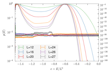
Details of the simulation techniques may be found in Ref. [6]. A two-step process is used, where estimates of an unknown weight function for configurations with system energy are iteratively improved. This replaces the Boltzmann weights that give the acceptance rate in traditional Metropolis Monte Carlo. In the first step the weights are adjusted so that the transition probabilities between configurations with different energies become constant, giving a flat energy histogram [16] as shown in Fig. 1 below.
The second step consists of a production run using the fixed weights produced iteratively in step one. This yields a time series of the energy, magnetization and the two different fuki-nuke observables and in the three possible different spatial orientations. With sufficient statistics such a time series together with the weights provides an 8-dimensional density of states by counting occurrences of and weighting them with the inverse of the weights fixed prior to the production run. Practically, estimators of the microcanonical expectation values of observables are used. When measuring the order parameters, measurements are carried out every sweeps, because the lattice must be traversed once to measure the order parameters in all spatial orientations which has a considerable impact on simulation times. Skipping intermediate sweeps gives less statistics, but the resulting measurements are less correlated in the final time series.
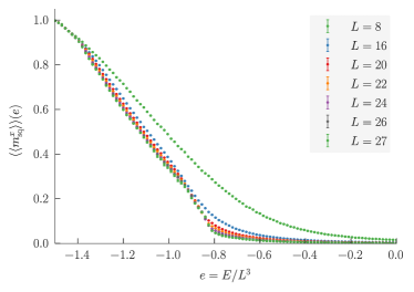
In Fig. 2, we show the estimators of the microcanonical expectation values of our magnetic observables ,
| (10) |
where the quantity is the number of states with energy and value of either the magnetization or one of the fuki-nuke order parameters.
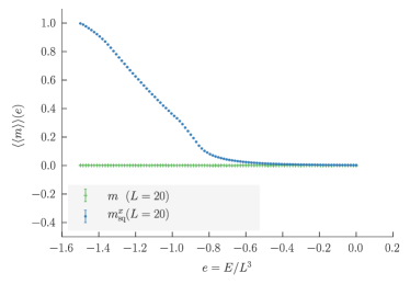
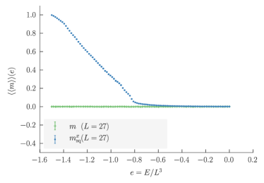
We get an estimator for by simply counting the occurrences of the pairs in the time series and weighting them with . For clarity in the graphical representation in Figs. 2 and 3 we used a partition of bins for the energy interval and an estimate for the statistical error of each bin was calculated by using Jackknife error analysis [17] with blocks of the time series.
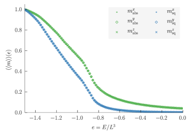
The fuki-nuke parameters are capable of distinguishing ordered and disordered states, unlike the standard magnetization, which is revealed by Fig. 2. It is also obvious from the first of Fig. 3 that the different orientations of the fuki-nuke parameters are equal for the isotropic gonihedric Ising model, which we show for . This confirms that the sampling is consistent in the simulation. We collect the microcanonical estimators for for several lattice sizes in the second of Fig. 3.
With the stored full time series and its weight function, we are able to measure the microcanonical estimators for arbitrary functions of the measured observables ,
| (11) |
which provides a convenient way of calculating higher-order moments. For canonical simulations reweighting techniques [15] allow system properties to be obtained in a narrow range around the simulation temperature whose width and accuracy are determined by the available statistics of typical configurations at the temperature of interest. Since multicanonical simulations yield histograms with statistics covering a broad range of energies (cf. Fig. 1) it is possible to reweight to a correspondingly broad range of temperatures. The canonical estimator at finite inverse temperature is thus obtained as
| (12) |
and Jackknife error analysis is again employed for an estimate of the statistical error.
The behaviour of and in a Metropolis simulation [12] is reproduced by the multicanonical data here as shown in Fig. 4.
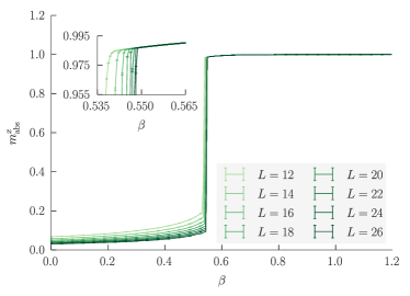
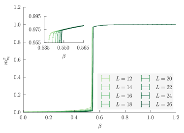
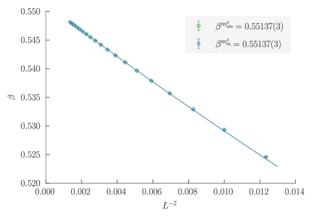
Sharp jumps are found near the inverse transition temperature, as expected for an order parameter at a first-order phase transition. The peaks in the associated susceptibilities provide a suitable estimate of the finite-size pseudo-transition point. We find that the peak locations for the different lattice sizes are fitted best by the modified first-order scaling laws with a leading correction appropriate for macroscopically degenerate systems discussed in detail in Refs. [5] and [6],
| (13) |
where smaller lattices were systematically omitted until a fit with quality-of-fit parameter bigger than was found. The fits presented have a goodness-of-fit parameter and degrees of freedom left. Fits to the other directions and fits to the peak location of the susceptibilities of give the same parameters within error bars and are of comparable quality.
The inverse temperature for the peak locations of the susceptibilities for both and is plotted against in Fig. 5 together with the best fit curve giving the quoted values for the scaling coefficients. The estimate of the phase transition temperature obtained here from the finite-size scaling of the fuki-nuke order parameter(s), , is in good agreement with the earlier estimate reported in Ref. [6] using fits to the peak location of Binder’s energy cumulant and specific heat and the value of where the energy probability density has two peaks of the same height or weight.
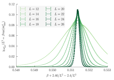
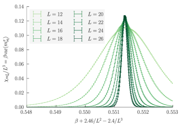
As a visual confirmation of the scaling, the normalized susceptibilities for various lattice sizes are plotted against (where the shifts are determined by the fitted scaling corrections) in Fig. 6. It is clear that the peak positions fall on the same point. In Fig. 7 we plot the peak values of both and divided by the system volume against .
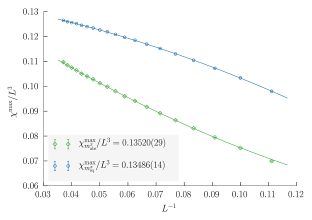
Empirically the plotted fits for the maximum values are
| (14) |
where we used all lattices with sizes greater than or equal to (with degrees of freedom left and a goodness-of-fit parameter of ) and
| (15) |
with (with degrees of freedom and ). The leading corrections of the peak value of the specific heat divided by the system volume are of order , so those for the susceptibility are already much stronger. Forcing a fit to leading corrections here gives slightly poorer fits and we cannot distinguish empirically. The constants, however, are stable around , and barely change with the various fits, showing that the proportionality factor of is independent of the leading corrections. By analogy with the maximum of the specific heat, [5, 6, 7] we expect for the extremal values of the susceptibilities
| (16) |
where the gaps of the fuki-nuke order parameters in the infinite system enter. This is consistent with the measurements since a value of implies , which is plausible from the insets in Fig. 4 giving an impression of the value of as and noting that .
4 Conclusions
The macroscopic degeneracy of the low-temperature phase in the plaquette gonihedric Ising model excludes standard magnetic ordering. However, consideration of the strongly anisotropic limit of the model suggests that a planar, fuki-nuke order may still be present. Multicanonical simulations of the model strongly support this suggestion, with the various fuki-nuke magnetizations all showing order parameter like behaviour. If the effects of the macroscopic low-temperature phase degeneracy on the corrections to scaling detailed in Refs. [5] and [6] are taken into account, the estimates for the transition point obtained from these fuki-nuke magnetizations are fully consistent with estimates obtained from energetic quantities. There are, however, stronger finite-size corrections to the peak value of the susceptibilities for the fuki-nuke order parameters.
Acknowledgements
This work was supported by the Deutsche Forschungsgemeinschaft (DFG) through the Collaborative Research Centre SFB/TRR 102 (project B04) and by the Deutsch-Französische Hochschule (DFH-UFA) under Grant No. CDFA-02-07.
References
-
[1]
G. K. Savvidy and F. J. Wegner, Nucl. Phys. B 413 (1994) 605;
G. K. Savvidy and K. G. Savvidy, Phys. Lett. B 324 (1994) 72;
G. K. Savvidy and K. G. Savvidy, Phys. Lett. B 337 (1994) 333;
G. K. Bathas, E. Floratos, G. K. Savvidy, and K. G. Savvidy, Mod. Phys. Lett. A 10 (1995) 2695;
G. K. Savvidy, K. G. Savvidy, and F. J. Wegner, Nucl. Phys. B 443 (1995) 565;
G. K. Savvidy and K. G. Savvidy, Mod. Phys. Lett. A 11 (1996) 1379;
G. K. Savvidy, K. G. Savvidy, and P. G. Savvidy, Phys. Lett. A 221 (1996) 233;
D. Johnston and R. P. K. C. Malmini, Phys. Lett. B 378 (1996) 87;
G. Koutsoumbas, G. K. Savvidy, and K. G. Savvidy, Phys. Lett. B 410 (1997) 241;
J. Ambjørn, G. Koutsoumbas, and G. K. Savvidy, Europhys. Lett. 46 (1999) 319;
G. Koutsoumbas and G. K. Savvidy, Mod. Phys. Lett. A 17 (2002) 751. - [2] A. Lipowski, J. Phys. A: Math. Gen. 30 (1997) 7365.
- [3] D. A. Johnston, A. Lipowski, and R. P. K. C. Malmini, in Rugged Free Energy Landscapes: Common Computational Approaches to Spin Glasses, Structural Glasses and Biological Macromolecules, ed. W. Janke, Lecture Notes in Physics 736 (Springer, Berlin, 2008), p. 173.
-
[4]
R. Pietig and F. Wegner, Nucl. Phys. B 466 (1996) 513;
R. Pietig and F. Wegner, Nucl. Phys. B 525 (1998) 549. - [5] M. Mueller, W. Janke, and D. A. Johnston, Phys. Rev. Lett. 112 (2014) 200601.
- [6] M. Mueller, D. A. Johnston, and W. Janke, Nucl. Phys. B 888 (2014) 214.
- [7] M. Mueller, W. Janke, and D. A. Johnston, Physics Procedia 57 (2014) 68.
-
[8]
Y. Hashizume and M. Suzuki, Int. J. Mod. Phys. B 25 (2011) 73;
Y. Hashizume and M. Suzuki, Int. J. Mod. Phys. B 25 (2011) 3529. - [9] M. Suzuki, Phys. Rev. Lett. 28 (1972) 507.
- [10] M. Mueller, W. Janke, and D. A. Johnston, Nucl. Phys. B 894 (2015) 1.
- [11] C. Castelnovo, C. Chamon, and D. Sherrington, Phys. Rev. B 81 (2010) 184303.
- [12] D. A. Johnston, J. Phys. A: Math. Theor. 45, 405001 (2012).
- [13] B. A. Berg and T. Neuhaus, Phys. Lett. B 267 (1991) 249; B. A. Berg and T. Neuhaus, Phys. Rev. Lett. 68 (1992) 9.
- [14] W. Janke, Int. J. Mod. Phys. C 03 (1992) 1137.
- [15] A. M. Ferrenberg and R. H. Swendsen, Phys. Rev. Lett. 61 (1988) 2635; W. Janke, in Computational Physics: Selected Methods – Simple Exercises – Serious Applications, eds. K. H. Hoffmann and M. Schreiber (Springer, Berlin, 1996), p. 10.
- [16] W. Janke, Physica A 254 (1998) 164; W. Janke, in Computer Simulations of Surfaces and Interfaces, eds. B. Dünweg, D. P. Landau, and A. I. Milchev, NATO Science Series, II. Math. Phys. Chem. 114 (Kluwer, Dordrecht, 2003), p. 137.
-
[17]
B. Efron,
The Jackknife, the Bootstrap and other Resampling Plans (Society for Industrial and Applied Mathematics, Philadelphia, 1982);
W. Janke, in Proceedings of the Euro Winter School Quantum Simulations of Complex Many-Body Systems: From Theory to Algorithms, eds. J. Grotendorst, D. Marx, and A. Muramatsu, NIC Series Vol. 10 (John von Neumann Institute for Computing, Jülich, 2002), p. 423;
M. Weigel and W. Janke, Phys. Rev. Lett. 102 (2009) 100601;
M. Weigel and W. Janke, Phys. Rev. E 81 (2010) 066701.