Interfacial thermal conduction and negative temperature jump in one-dimensional lattices
Abstract
We study the thermal boundary conduction in one-dimensional harmonic and lattices, both of which consist of two segments coupled by a harmonic interaction. For the ballistic interfacial heat transport through the harmonic lattice, we use both theoretical calculation and molecular dynamics simulation to study the heat flux and temperature jump at the interface as to gain insights of the Kapitza resistance at the atomic scale. In the weak coupling regime, the heat current is proportional to the square of the coupling strength for the harmonic model as well as anharmonic models. Interestingly, there exists a negative temperature jump between the interfacial particles in particular parameter regimes. A nonlinear response of the boundary temperature jump to the externally applied temperature difference in the lattice is observed. To understand the anomalous result, we then extend our studies to a model in which the interface is represented by a relatively small segment with gradually changing spring constants, and find that the negative temperature jump still exist. Finally, we show that the local velocity distribution at the interface is so close to the Gaussian distribution that the existence/absence of local equilibrium state seems unable to determine by numerics in this way.
pacs:
05.70.Ln, 44.10.+i, 05.60-kI Introduction
Since the pioneering observation between liquid helium and a metal Kapitza (1941), thermal boundary resistance, namely, Kapitza resistance, has been extensively studied theoretically and experimentally Swartz and Pohl (1989). With the rapid development of modern electronic technology, there has been much need and interest in understanding the fundamental nature of thermal boundary conductance since it has been a significant obstacle in designing the micro- or nano- scale electronic chips. Two phenomenological models, the acoustic mismatch model Little (1959) and diffuse mismatch model Swartz and Pohl (1989), have been proposed to study the mechanism of the thermal boundary conductance. However, due to the neglecting of atomic details at the interface, they both offer limited accuracy, particularly, for nanoscale interfacial resistance Lumpkin et al. (1978). To understand the mechanism of thermal boundary conductance at the atomic level, many studies have been done in one-dimensional lattices via different methods Lumpkin et al. (1978); Zhang et al. (2011); He et al. (2009). Most of the previous studies focus on the effect of the interface on the steady-state heat flux and little attention has been paid to the temperature jump between the interface from the atomic viewpoint.
On the other hand, heat conduction in low-dimensional dynamical systems has become the subject of a large number of theoretical and experimental studies in recent years Lepri et al. (2003); Dhar (2008); Wang et al. (2008). An exact approach to interacting Hamiltonian systems is so far unavailable except for harmonic crystals. A meaningful definition of local temperature depends on the local thermal equilibrium and it is difficult to give a microscopic derivation of the condition in general Bonetto et al. (2000). With the usual definition of local temperature i.e., the mean local kinetic energy, the temperature profile may show some unexpected features, such as the temperature oscillations in the steady state of alternate mass hard particle gas Garrido et al. (2001), in the Fermi-Pasta-Ulam chain Mai et al. (2007) and in harmonic chain with alternating mass Kannan et al. (2012).
In the present study, we study the heat flux and temperature jump at the interface as to gain insights of the Kapitza resistance at the atomic scale via theoretical calculations and molecular dynamics simulations. We find that there exists a negative temperature jump between the interfacial particles in particular parameter regimes. A nonlinear response of the boundary temperature jump to the externally applied temperature difference in the lattice is observed. Note that, although the interface between two segments is not well defined in one-dimensional Hamiltonian systems, our studies can give some insights into the thermal boundary resistance in real systems.
The paper is organized as follows. In Sec. II we define the model and give the methods for theoretical calculations and molecular dynamics simulations. In Sec. III we demonstrate the existence of negative temperature jump in both the harmonic and model. Finally, we give a brief summary and discussion in Sec. IV.
II Model and Methods
We study the non-equilibrium steady state of a one dimensional chain consisting of two coupled lattice,
| (1) |
The Hamiltonian for the left and right segments are given by
| (2) | |||
where denotes the displacement of the -th particle from its equilibrium position. Fixed boundary conditions are taken, i.e., . The particle and at the two ends are connected to the heat baths at temperature and , respectively. The heat baths are modeled by the Langevin equations corresponding to Ohmic baths, i.e., the self energy of the baths are Dhar (2008).
When , the on-site potential and inter-particle interaction are all quadratic. In the classical limitation, the steady heat current from left to right reservoir can be given by the Langevin equations and Green’s function (LEGF) method Dhar (2008); Dhar and Roy (2006)
| (3) |
with
| (4) | |||
| (5) |
where and denote the mass matrix and force constant matrix of the system. Note that are all matrices for one-dimensional systems. The only non-zero element of are respectively and . is the coupling strength of the first and -th particle to the left and right reservoirs, respectively. The velocity-velocity correlation and position-velocity correlation are:
| (6) | |||
| (7) | |||
The correlation function can be used to define local energy density which can in turn be used to define the local temperature, i.e.,
| (8) |
and gives the local heat current density Dhar and Shastry (2003); Dhar (2001); Rubin and Greer (1971); O’Connor and Lebowitz (1973). We integrate Eq. (3) and Eq. (6) numerically to obtain the steady state heat current and local temperature, for which the rectangular method is used Press et al. (2007). We also verify that the local current, obtained by integrating Eq. (7) numerically, is the same along the chain, which is one of the properties in the steady state.
When , we apply the non-equilibrium molecular dynamics simulation(NEMD) to the system, for which the Langevin heat baths are used at the two ends of the chain. The equations of motion are given by
| (9) |
where and . The noise terms denotes a Gaussian white noise with zero mean and variance of . The local heat flux is given by , where and the notion denotes a steady-state average. The equations of motion (Eq. (9)) are integrated by using a second-order Stochastic Runge-Kutta algorithm Honeycutt (1992). At steady states, the numerically computed local heat flux is always constant along the chain, and the local temperature is defined as . To compute the boundary temperature jump, i.e., , the relaxation and average time must be both long enough. In what follows we set , and .
III Results and Discussions
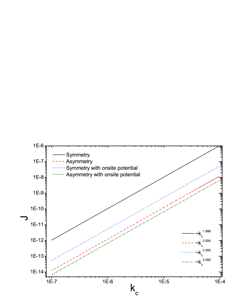
For many devices of several segments, interfacial coupling is pretty weak, which indicates that is far less than and in our model. So it is desirable to study the thermal transport through atomic chains in the weak coupling regime. It has been shown that Hu et al. (2006) the heat current is proportional to the square of the coupling strength in one-dimensional weakly-coupled chain with the Morse on-site potential by a phenomenological analysis. Does this square-law relation between heat current and coupling strength is still valid in the weak coupling limit when the anharmonic on-site potential is absent? As shown in Fig.1, we plot the heat current as a function of the coupling strength in the weak coupling limit by integrating Eq. (3) numerically. It turns out that the square law relation is still valid when the anharmonicity is absent. Further more, the square law relation still holds when the system consists of symmetrical/asymmetrical segments with/without an on-site potential.
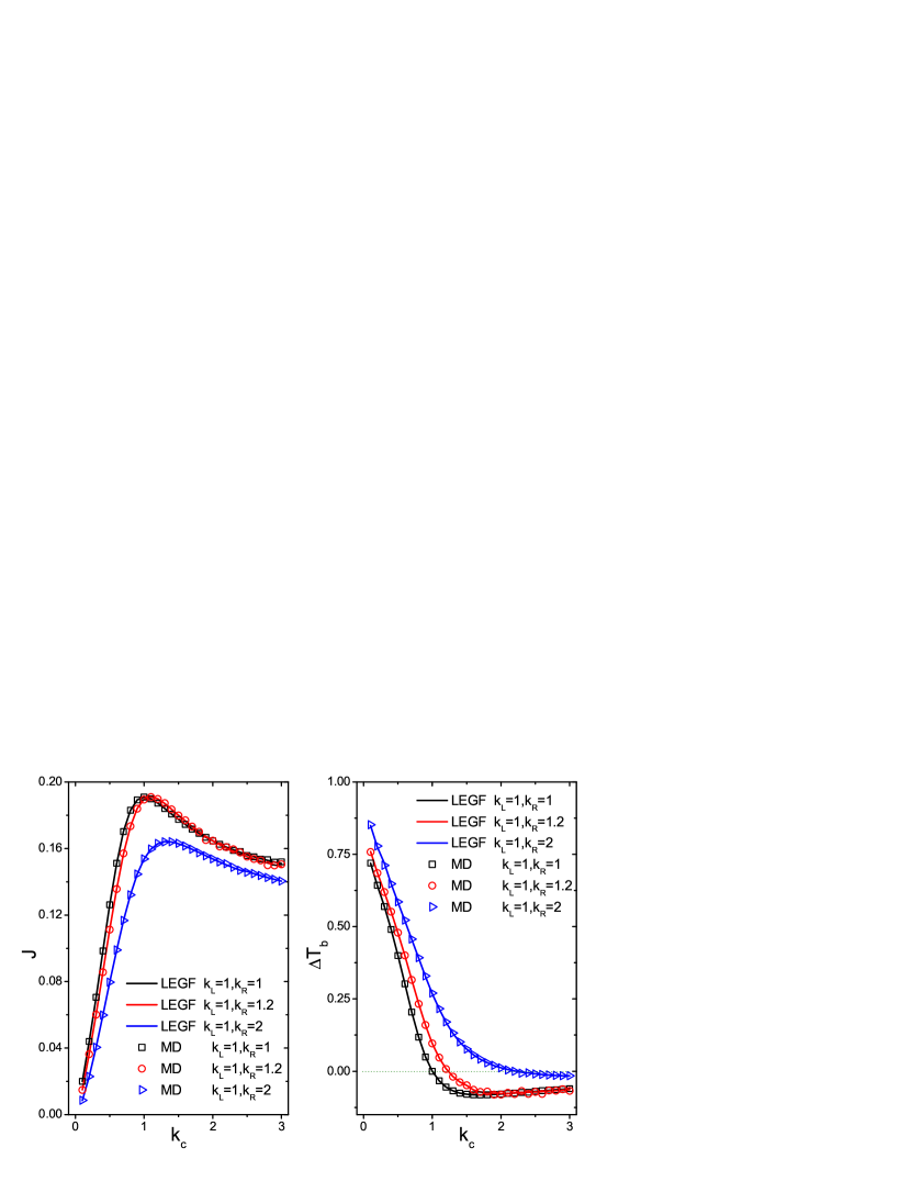
Fig. 2 shows the steady-state heat current and the boundary temperature jump as a function of the coupling strength . The reason to carry out both theoretical calculation and NEMD simulation is to verify that the results we obtained are from physical reasons rather than uncertain numerical reasons because the temperature jump between the -th particle and the -th particle requires a highly accurately performed simulation for its sensitive to heat fluctuation when approaches to . By inspecting the figure, we can see that theoretical calculations and MD simulations agree well with each other. The heat current increases at first, then arrives at a maximum value, and then slightly decreases with the increase of . As depicted in Fig. 2, the maximum heat current occurs at , which agrees with the result obtained in Zhang et al. (2011) by the scattering boundary method. Furthermore, both theoretical calculations and MD simulations indicate that there is a negative boundary temperature jump, i.e., , when approaches to . The word “negative” is in contrast with “normal”heat conduction that the direction of the heat flow is from hot to cold regions. In fact, similar negative temperature jumps occurs in several systems, for example, the temperature jump between the second and third particle, and between -th and -th particle in the uniform harmonic chain Lepri et al. (2003) coupled with reservoirs, and the temperature oscillations in the steady state of hard particle gas Garrido et al. (2001), the Fermi-Pasta-Ulam chain Mai et al. (2007), the harmonic chain Kannan et al. (2012) with alternating mass.
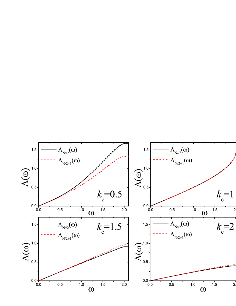
To understand the negative temperature jump at the interface, we need to inspect the concept of the local temperature further. The local temperature of the -th particle can be written as , with
| (10) |
and is the top boundary of the phonon spectra. The kinetic energy of a particle gets contributions from all the modes, and the net result depends on the distribution of energy in the different modes. As shown in Fig. 3, we plot the contribution of normal modes to the local temperature for the -th and -th particles by integrating Eq. (10) numerically. As we can see, “equipartition” among phonon modes, i.e., each normal mode shares the same average kinetic energy, is not satisfied for and shown by the nonlinear behaviors of () in the high frequencies region. Surprisingly, for the case of , exhibit almost linear behavior with the increasing of , indicating that the contribution to the local temperature from possible phonon modes are closely equivalent. Comparing with , we can see that the high frequency normal modes are suppressed more dramatically than the low frequency normal modes for and , and the turning of and in the high frequencies region indicates the negative temperature jump between the -th and -th particle.
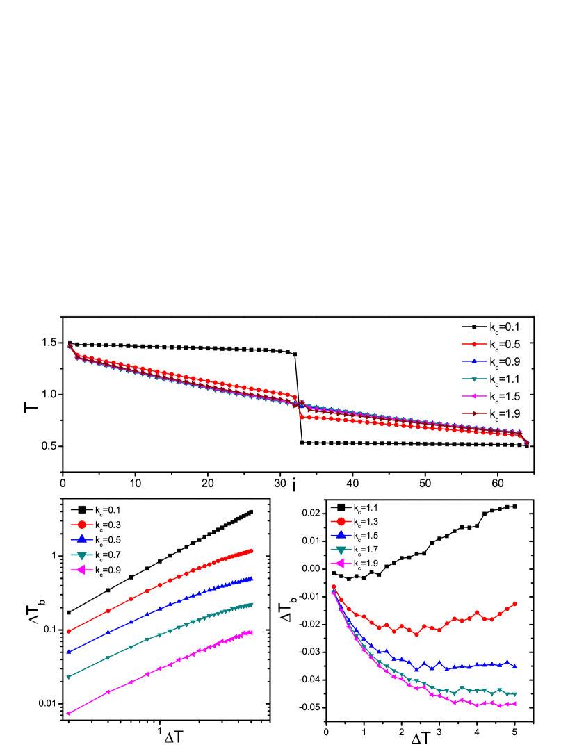
It would be interesting to see if the negative temperature jump is an artificial effect due to the integrability of the harmonic system. Thus we conduct similar studies in the lattice, which has additional nonlinear on-site potential on each site in comparison with the harmonic system. We plot the boundary temperature jump as a function of the external temperature difference and some typical temperature profiles in Fig. 4. One can see that the boundary temperature jump is proportional to for and proportional to for when is small, which are typical linear-response behaviors shown in harmonic models. With the increasing of , the linear behavior of no longer holds for the lattice. Note that negative temperature jump occurs when and the absolute value of nonlinearly increases as increases.
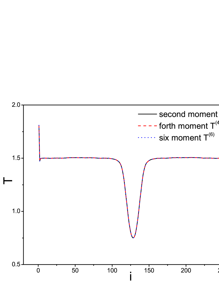
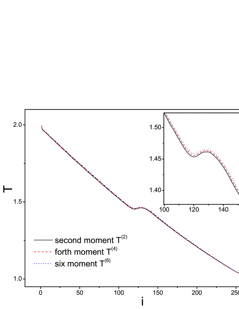
So far our discussions is based on the model consisting of two segments with a single harmonic coupling, which inevitably leads to the argument that the origin of negative temperature jump comes from the ill-defined interface of the two-segment model with a sharp discontinuity of the interfacial coupling. In what follows we propose an extended model to show that it is not the case. Actually, in a practical consideration, the interface may be a junction which is small compared with the two sub-lattices. So we divide our system into three regions, say, two sub-lattices and a junction. The particle number of the junction is small compared with the two sub-lattices. The spring constant of the intermediate segment varies smoothly, which is done by setting the spring constants of the intermediate junction by , where represents the index of particles. The NEMD simulation results of harmonic and lattices are presented in Fig. 5 and Fig. 6, respectively. As we can see, negative temperature gradient still exists for both harmonic and lattices within the interfacial segment.
As mentioned above, a meaningful local temperature can be defined only in systems exhibiting local thermal equilibrium. And we known that, if the system can exhibit local thermal equilibrium, the local distribution should be gaussian and all even moments can be obtained based on the second moment. We can then use , , and to define local temperature equivalently. So we carry out NEMD simulation for both the harmonic and lattice, and plot the local temperature defined by the first three even moments of velocity, namely, the second, fourth and sixth moment in Fig. 5 and Fig. 6. To our surprise, the local temperature defined by , and at the boundary particles agree well with each other. The deviation at the interface is not significant in comparison with that inside segments. The result indicates the local distribution is or at least very close to the Gaussian, which cannot be well distinguished by numerics and should recourse to more careful theoretical studies of local distribution in the future.
IV SUMMARY
We have studied interfacial thermal conductance in one-dimensional inhomogeneous systems by using both theoretical calculations and MD simulations. In the weak coupling limit, theoretical calculations show that the heat current is proportional to the square of the coupling strength in the absence of anharmonicity. A negative temperature jump between the interfacial particles occurs in both the harmonic and lattices. As to understand the counterintuitive observation, we have investigated the contribution of normal modes to the local temperature at the interface. It is shown that the high frequency modes make dominant contribution when the coupling strength is small, however, the contribution of each mode is almost equivalent when the coupling strength is strong. We have confirmed the occurring of the negative temperature jump is not trivially artificial due to the integrability of the system or the sharp discontinuity of the interfacial coupling by extending the system to a model consisting of two sub-lattices and an intermediate junction for both the harmonic and lattices.
One should reexamine the notion of temperature as to understand the anomalous negative temperature jump, which seemingly indicats that heat flows against a local temperature gradient in a small scale. On the one hand, from the viewpoint of traditional thermodynamics, local temperature should be defined in a “cell” which should be macroscopically infinitesimal but contain enough microscopic degrees of freedom. Such kind of cell is, strictly speaking, not well defined for our microscopic model due to the large atomic-scale fluctuations and the word ”local” defined for a single oscillator loses its inherent meaning. On the other hand, we stress that the traditional definition of local temperature with respect to the kinetic energy of an oscillator is still in the framework of equilibrium thermodynamics. The anomalous phenomenon may partly comes from the definition as used here, which lacks a complete description of the nonequilibrium steady state. A new definition of “nonequilibrium temperature” might be taken into consideration on this count Morriss and Rondoni (1999); Casas-V zquez and Jou (2003), especially when one take notice of the temperature profile for the middle region of the intermediate junction, which is anomalously smaller than as shown in Fig. 5. However, whether the concept of (local) temperature can be extrapolated beyond local equilibrium or should be modified in the nonequilibrium systems is still an open question.
Acknowledgements.
The authors thank Y. Zhang, J. Wang, and H. Zhao for helpful discussioins and Xiamen Supercomputer center for using its computing facilities. This work was financially supported by NSFC No. 11047185, No. 11105112 and No. 11335006.References
- Kapitza (1941) P. L. Kapitza, J. Phys. USSR 4, 181 (1941).
- Swartz and Pohl (1989) E. T. Swartz and R. O. Pohl, Rev. Mod. Phys. 61, 605 (1989).
- Little (1959) W. Little, Can. J. Phys 37, 334 (1959).
- Lumpkin et al. (1978) M. E. Lumpkin, W. M. Saslow, and W. M. Visscher, Phys. Rev. B 17, 4295 (1978).
- Zhang et al. (2011) L. Zhang, P. Keblinski, J.-S. Wang, and B. Li, Phys. Rev. B 83, 064303 (2011).
- He et al. (2009) D. He, S. Buyukdagli, and B. Hu, Phys. Rev. B 80, 104302 (2009).
- Lepri et al. (2003) S. Lepri, R. Livi, and A. Politi, Phys. Rep. 377, 1 (2003).
- Dhar (2008) A. Dhar, Adv. Phys. 57, 457 (2008).
- Wang et al. (2008) J.-S. Wang, J. Wang, and J. T. Lü, Eur. J. Phys. B 62, 381 (2008).
- Bonetto et al. (2000) F. Bonetto, J. Lebowitz, and L. Rey-Bellet, “Fourier s law: A challenge to theorists, in Mathematical Physics 2000,” (Imperial College Press, London, 2000) p. 128.
- Garrido et al. (2001) P. L. Garrido, P. I. Hurtado, and B. Nadrowski, Phys. Rev. Lett. 86, 5486 (2001).
- Mai et al. (2007) T. Mai, A. Dhar, and O. Narayan, Phys. Rev. Lett. 98, 184301 (2007).
- Kannan et al. (2012) V. Kannan, A. Dhar, and J. L. Lebowitz, Phys. Rev. E 85, 041118 (2012).
- Dhar and Roy (2006) A. Dhar and D. Roy, J. Stat. Phys. 125, 805 (2006).
- Dhar and Shastry (2003) A. Dhar and B. S. Shastry, Phys. Rev. B 67, 195405 (2003).
- Dhar (2001) A. Dhar, Phys. Rev. Lett. 86, 5882 (2001).
- Rubin and Greer (1971) R. J. Rubin and W. L. Greer, J. Math. Phys. 12, 1686 (1971).
- O’Connor and Lebowitz (1973) A. J. O’Connor and J. L. Lebowitz, J. Math. Phys. 15, 692 (1973).
- Press et al. (2007) W. H. Press, S. A. Teukolsky, W. T. Vetterling, and B. P. Flannery, Numerical Recipes: The Art of Scientific Computing, 3rd ed. (Cambridge University Press, New York, 2007).
- Honeycutt (1992) R. L. Honeycutt, Phys. Rev. A 45, 600 (1992).
- Hu et al. (2006) B. Hu, D. He, L. Yang, and Y. Zhang, Phys. Rev. E 74, 060101 (2006).
- Morriss and Rondoni (1999) G. P. Morriss and L. Rondoni, Phys. Rev. E 59, R5 (1999).
- Casas-V zquez and Jou (2003) J. Casas-V zquez and D. Jou, Rep. Prog. Phys. 66, 1937 (2003).