Analytical model for non-thermal pressure in galaxy clusters - III. Removing the hydrostatic mass bias

Abstract

Non-thermal pressure in galaxy clusters leads to underestimation of the mass of galaxy clusters based on hydrostatic equilibrium with thermal gas pressure. This occurs even for dynamically relaxed clusters that are used for calibrating the mass-observable scaling relations. We show that the analytical model for non-thermal pressure developed in Shi & Komatsu (2014) can correct for this so-called ‘hydrostatic mass bias’, if most of the non-thermal pressure comes from bulk and turbulent motions of gas in the intracluster medium. Our correction works for the sample average irrespective of the mass estimation method, or the dynamical state of the clusters. This makes it possible to correct for the bias in the hydrostatic mass estimates from X-ray surface brightness and the Sunyaev-Zel’dovich observations that will be available for clusters in a wide range of redshifts and dynamical states.

1 Introduction

Galaxy clusters promise great statistical power as a low redshift cosmological probe, if their masses are estimated accurately (Allen, Evrard & Mantz, 2011). A bias in the mass estimation poses the most serious challenge to the success of cluster cosmology. For example, the recently reported tension in cosmological inferences from the cosmic microwave background (CMB) and galaxy clusters measured by the Planck satellite, the so-called ‘Planck CMB-Cluster tension’ (Planck Collaboration V., 2013; Planck Collaboration XXIV., 2015), may point to new physics, but it may also reflect the urgent need for better understanding and correction for systematic biases (see e.g. von der Linden et al., 2014; Leistedt, Peiris & Verde, 2014; Donahue et al., 2014; Israel et al., 2015).

The most prominent astrophysical bias has to do with the assumption of hydrostatic equilibrium (HSE) of the intracluster medium (ICM) inside the gravitational potential. HSE no longer holds in the presence of non-thermal sources of pressure. Hydrodynamical simulations show significant pressure associated with bulk and turbulent motions of the gas, which leads to a ‘HSE mass bias’ of order ten percent or more in the mass estimates of individual clusters (e.g., Kay et al., 2004; Rasia et al., 2006, 2012; Nagai, Vikhlinin & Kravtsov, 2007; Piffaretti & Valdarnini, 2008; Lau, Kravtsov & Nagai, 2009; Meneghetti et al., 2010; Nelson et al., 2012; Nelson, Lau & Nagai, 2014).

As the amplitude of non-thermal pressure can hardly be measured directly by observations, one has to resort to theoretical estimations to correct for this bias. To this end, we have developed a physically motivated analytical model for non-thermal pressure in the ICM (Shi & Komatsu, 2014, SK14 hereafter). Given the accretion history of the cluster, the model predicts the amplitude of non-thermal pressure and its radial, mass, and redshift dependencies. The model successfully reproduces the average non-thermal pressure profiles seen in cosmological hydrodynamical simulations (Battaglia et al., 2012), the average thermal pressure profile measured by Planck (Arnaud et al., 2010), as well as non-thermal pressure profiles of individual clusters in hydrodynamical simulations (Shi et al., 2015, SKNN15 hereafter).

In this paper, we study the ability of the SK14 model in correcting the HSE mass estimation by testing it on simulated clusters in a set of high-resolution cosmological hydrodynamical simulations (Nelson, Lau & Nagai 2014), with special attention paid to the dynamical state of galaxy clusters.

The dynamical state of a cluster influences its mass estimation in two ways. First, the more dynamically relaxed a cluster is, the smaller its non-thermal pressure (e.g. SK14; Nelson et al. 2014), and thus the smaller its HSE mass bias. Second, the cluster profiles are smoother when a cluster is dynamically more relaxed, which gives a better precision in the mass estimation.

In the early days, HSE mass estimates were applied to clusters irrespective of their dynamical state (e.g. Reiprich & Böhringer, 2002). These studies use X-ray surface brightness data and make the assumption that the ICM is isothermal. After the recognition that gas temperature decreases systematically with increasing radius outside the cluster core region, precise HSE mass estimates require also spatially-resolved, high signal-to-noise gas temperature measurements, which are harder to obtain especially out to high redshifts.

The current cluster mass estimates for a large sample of clusters are mostly performed statistically (rather than individually) using scaling relations between the mass and spatially-averaged observables, such as the mean X-ray temperature, luminosity, or their combination, and the Sunyaev-Zel’dovich (SZ) effect (Sunyaev & Zeldovich, 1970, 1972) averaged over certain cluster radii (e.g. Vikhlinin et al. 2009; Andersson et al. 2011; Bender et al. 2014; Planck Collaboration XX. 2014, see also Giodini et al. 2013 for a review). In this context, HSE mass estimates are usually performed only on a small sample of dynamically relaxed clusters where the bias from non-thermal pressure is minimized, and are used for observationally calibrating the scaling relations with the hope that the adopted scaling relation is robust against varying dynamical states (which holds true for some scaling relations, see Kravtsov, Vikhlinin & Nagai 2006).

However, even for relaxed clusters, non-thermal pressure is expected to be non-negligible because non-thermal motions are continuously sourced by the mass accretion and are never fully thermalized, especially at the cluster outskirts (SK14; Nelson et al. 2014). Therefore, it is important to study the correction of HSE mass bias induced by non-thermal pressure for dynamically relaxed clusters. This is one of the primary goals of this paper.

In recent years, the advances in SZ observations make it possible to estimate HSE masses using X-ray surface brightness combined with the gas pressure profiles probed by the SZ effect, without the expensive X-ray temperature measurements. This will make individual cluster mass estimates for a large number of clusters possible out to high redshifts, and this time with high precision to large radii thanks to the relative insensitivity of the SZ effect to gas density. In light of these observational advances, another goal of this paper is to study the possibility of correcting HSE mass bias for a population of clusters in a wide range of redshifts and dynamical states.

The rest of the paper is organized as follows: we introduce our method of correcting non-thermal pressure in cluster mass estimation in Sect. 2.1, where we discover the necessity of regulating the input cluster profiles by fitting or smoothing. Then we present four methods for regularizing the profiles in Sect. 2.2 and 2.3 and apply them to our simulated clusters. After introducing the way we select subsample of clusters based on their dynamical state in Sect. 2.4, we present our results in Sect. 2.5 and conclude in Sect. 3. In the two appendices we study the effect of velocity anisotropy (Appendix A) and how an error on the pressure profile propagates to an error on the mass (Appendix B).

2 HSE Mass estimate and its correction

2.1 Method

The assumption of HSE relates the thermal pressure $P_{\rm th}$ that is observable from both X-ray and SZ observations to the hydrostatic mass $M_{\rm HSE}$ as

$$M_{\rm HSE}(<r)\equiv-\frac{r^{2}}{G\rho_{\rm gas}(r)}\frac{\partial P_{\rm th}}{\partial r}\,,$$ (1)

where $\rho_{\rm gas}$ is the gas density. Since the total pressure in the ICM, $P_{\rm tot}\equiv P_{\rm th}+P_{\rm nth}$ where $P_{\rm nth}$ is non-thermal pressure support, is greater than $P_{\rm th}$ by definition, $M_{\rm HSE}$ is an underestimate of the true mass. We thus define the ‘corrected mass’ $M_{\rm corr}$ as

$$M_{\rm corr}(<r)\equiv-\frac{r^{2}}{G\rho_{\rm gas}(r)}\frac{\partial P_{\rm tot}}{\partial r}\,.$$ (2)

This $M_{\rm corr}$ is expected to be close to an unbiased estimate of the total mass when the non-thermal pressure support is the dominant source of the HSE mass bias, as is the case found in hydrodynamical simulations at least for regions within $r_{500}$ (e.g. Lau, Nagai & Nelson, 2013; Nelson et al., 2014).

Cluster masses are usually defined with respect to a radius $r_{\Delta}$, within which the mean density equals e.g. $\Delta=500$ times the critical density of the Universe $\rho_{\rm crit}$,

$$M_{\Delta}\equiv\frac{4\pi r_{\Delta}^{3}}{3}\rho_{\rm crit}\Delta\,.$$ (3)

Solving for $M_{\Delta}$ using equation (1) or (2) is equivalent to finding the corresponding radius $r_{\Delta}$ from a spherically-averaged ‘overdensity’ profile defined by

$$\mathbf{\Delta}(r)\equiv\frac{1}{\rho_{\rm crit}}\frac{3GM(<r)}{4\pi r^{3}}=-\frac{3}{4\pi\rho_{\rm crit}}\frac{1}{r\rho_{\rm gas}(r)}\frac{\partial P}{\partial r}\,,$$ (4)

with the implicit relation $\mathbf{\Delta}(r_{\Delta})=\Delta$. Here, $P$ is either $P_{\rm th}$ or $P_{\rm tot}$. An error on the pressure gradient due to neglecting $P_{\rm nth}$ will lead to an error on $M_{\Delta}$ through an incorrect estimation of $r_{\Delta}$.

Figure 1: Spherically-averaged overdensity profiles (equation 4) with respect to the critical density, $\mathbf{\Delta}(r)$, of a simulated cluster. The horizontal dotted lines show $\Delta=500$ and 200. The true overdensity profile (black solid line) is calculated from the mass profile in the simulation, whereas the estimated profiles are calculated from spherically-averaged gas density and pressure profiles in the simulation using equations (1) and (2) (red and blue lines, respectively). Structures and noises in the gas density and pressure profiles are greatly amplified by the derivative and division procedures required in computing the overdensity profile (dashed lines), suggesting the need for fitting (solid lines) or smoothing.

We apply the HSE and corrected mass estimates to a mass-limited sample of 65 galaxy clusters with $M_{500}>2.2\times 10^{14}h^{-1}\mbox{$\,{\rm M}_{\sun}$}$ at redshift $z=0$ and their most massive progenitors at $z=0.6$ in the Omega500 simulation (Nelson et al., 2014), an Eulerian hydrodynamic cosmological simulation. Radiative cooling, star formation and feedback are not included in the current runs of the Omega500 simulation. These additional physics are crucial for reproducing the observed behaviors of cluster cores. They also affect the detailed shapes of the thermo-dynamical profiles in the bulk of ICM, especially for low mass systems. For low mass clusters and galaxy groups, testing non-thermal pressure and cluster mass estimations would be better performed with simulations with cooling and feedback. However, these additional physics do not change the overall shape of the ICM profiles outside the cluster core (e.g. Nagai, Kravtsov & Vikhlinin, 2007). In particular, the velocity dispersion of the gas and fraction of non-thermal pressure at around $r_{\rm 500}$ are consistent to typically $<$10% between simulations with and without cooling and feedback (Nagai et al., 2013; Nelson, Lau & Nagai, 2014) even for clusters with relatively low masses $M_{\rm 200}\approx 2\times 10^{14}$$\,{\rm M}_{\sun}$(corresponding to $M_{\rm 500}\approx 10^{14}h^{-1}\mbox{$\,{\rm M}_{\sun}$}$) (Battaglia et al., 2012). Therefore, non-radiative simulations are adequate for our purpose. We refer to Sect. 2 of SKNN15 and references therein for further descriptions of the simulation and the cluster sample used in this paper. Small clumps have been removed when constructing the one-dimensional cluster profiles by excluding high-density tail in the probability distribution of gas densities using the Zhuravleva et al. (2013) method.

We first compute the overdensity profile $\mathbf{\Delta}(r)$ from simulated profiles with equation (4), taking $P=P_{\rm th}$ for $M_{\rm HSE}$ and $P=P_{\rm th}/(1-f_{\rm nth})$ for $M_{\rm corr}$. We then use equation (3) to compute $M_{\rm 500}$. Here, $f_{\rm nth}$ is the ‘non-thermal fraction’ defined by $f_{\rm nth}\equiv P_{\rm nth}/(P_{\rm th}+P_{\rm nth})$. We compute $f_{\rm nth}$ of each cluster using the SK14 model and the mass accretion history of the cluster measured from the simulation (see SKNN15 for details).

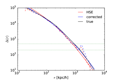
Numerically calculating a cluster mass using equation (4) is not trivial, as taking derivative of pressure and dividing by density would amplify small-scale structures and noise. If we apply no regulation of the simulated profiles other than a cubic-spline interpolation when computing the derivative of the pressure profile, the resulting overdensity profile will be far from smooth (dashed lines in Fig. 1), despite that the gas density and pressure profiles are rather smooth after clumps are removed. In the previous X-ray studies, the observed gas density and temperature profiles are often fit to parametric models to reduce this noise (e.g. Pointecouteau, Arnaud & Pratt, 2005; Vikhlinin et al., 2006; Schmidt & Allen, 2007). Non-parametric smoothing methods have also been adopted in simulation studies (Lau, Kravtsov & Nagai, 2009; Nelson et al., 2014).

Here we use and compare four approaches: one based on cubic spline smoothing, and the others based on fitting pressure and density to different parametrized models. For the parametrized models, we further compare two fitting ranges.

2.2 Cubic spline smoothing

First, we compute the overdensity profile (equation 4) from simulated gas density and pressure profiles with cubic spline interpolation applied to pressure when taking a derivative, $\partial P/\partial r$. We then smooth the computed $\log\mathbf{\Delta}(\log r)$ profile with a cubic-spline smoothing algorithm described in Dierckx (1993). The algorithm fits the data points with a piece-wise cubic spline with an increasing number of nodes, until the input constraint on the value of $\chi^{2}$ statistic is satisfied. We use the constraint that $\chi^{2}$ divided by the number of degrees of freedom is less than 0.04. This constraint is chosen to minimize the variance of $M_{\rm HSE}/M_{\rm corr}$ while not biasing the sample mean.

When estimating $M_{\rm 500}$ with the smoothing method, a large radial range of data around the true $r_{\rm 500}$ is needed to guarantee that the estimated $\Delta(r)$ profile covers $\Delta=500$. Therefore, we apply this method only to rather relaxed clusters using data on the radial range of [0.1, 1.5] $r_{\rm 500}^{\rm true}$.

2.3 Parametrized models

Next, we fit parametrized models to the pressure and gas density profiles and estimate masses. We fit pressure rather than temperature because pressure is the quantity that directly enters the HSE and corrected mass estimation. Also, thermal pressure is the quantity that the thermal Sunyaev-Zel’dovich (SZ) effect (Sunyaev & Zeldovich, 1970, 1972) directly probes, so fitting gas density and pressure may be a better option when applying to combined SZ and X-ray data.

The data points used in the fit are equally spaced logarithmic bins with uniform weighting on the radial range of either [0.1, 1] $r_{\rm 500}^{\rm true}$ or [0.1, 1.5] $r_{\rm 500}^{\rm true}$. These are the typical radial ranges of the currently available data on well-resolved clusters used for the mass calibration.

2.3.1 Model ‘VV’

We first use the model presented in Vikhlinin et al. (2006), which is based on an isothermal $\beta$ model (Cavaliere & Fusco-Femiano, 1978) with modifications capturing the cool cores and the observed steepening of the gas density profile at large radii. Here we ignore the modification for the cool cores, both because cool cores are non-existent in our simulated clusters, and that our focus is on the outer region of the clusters, especially around $r_{\rm 500}$ where we determine their masses. The resulting simplified model is:

$$\rho_{\rm gas}(r)\propto\frac{1}{(1+r^{2}/r_{c}^{2})^{\frac{3\beta}{2}}}\frac{1}{(1+r^{\gamma_{d}}/r_{d}^{\gamma_{d}})^{\frac{\epsilon}{2\gamma_{d}}}}\,,$$ (5)

and

$$P(r)\propto\rho_{\rm gas}(r)\frac{(r/r_{t})^{-a}}{(1+r^{b}/r_{t}^{b})^{c/b}}\,.$$ (6)

Following Vikhlinin et al. (2006), we fix $\gamma_{d}=3$. After this, this model still has 10 parameters (including 2 for normalization), and is highly nonlinear, suggesting the possible existence of local minima in the $\chi^{2}$ function.

For all the parametrized models, we fit the simulated gas density and pressure profiles to the models by searching for the global minimum of the $\chi^{2}$ function in a wide parameter range. Here, we set $0\leq\epsilon\leq 5$, $0\leq\beta\leq 10$, $-1\leq a\leq 5$, $0\leq b\leq 10$, $0\leq c\leq 10$, and $r_{c}$ and $r_{t}$ being less than 1 Mpc/h.

2.3.2 Model ‘VG’

The Vikhlinin model was designed to fit gas density and temperature of the ICM. It is then not surprising that the fitting form for the pressure (equation 6) is rather redundant. Here, instead, we use a generalized Navarro-Frenk-White (GNFW) profile (Zhao, 1996) for pressure, as suggested by Nagai, Kravtsov & Vikhlinin (2007):

$$P(r)\propto\frac{1}{r^{\gamma}\left[1+(r/r_{p})^{1/\alpha}\right]^{\alpha(\beta-\gamma)}}\,.$$ (7)

This simpler form already has enough flexibility to describe the shape of the observed thermal pressure profiles (e.g. Arnaud et al., 2010), as well as our simulated $P_{\rm th}$ and $P_{\rm tot}$. Here we further fix $\gamma=0$ which provides an adequate fit to all our simulated clusters. For the GNFW parameters, we search for the best fit values within $0.5\leq\alpha\leq 2$, $3\leq\beta\leq 8$ and $r_{p}$ between 10 kpc/h and 1 Mpc/h.

For the gas density we still use the Vikhlinin formula (equation 5). The result is a 9-parameter model.

2.3.3 Model ‘NG’

An ideal parametrized model fits the data with enough flexibility with a minimum number of fitting parameters. The way to achieve this is to utilize existing knowledge or well-founded assumptions on the underlying physical system that the data represent.

Here we try to do so by assuming that the total mass density profile follows an NFW profile (Navarro, Frenk & White, 1996). The gravitational acceleration, $g(r)$, is then given by

$$g(r)=\frac{GM(<r)}{r^{2}}\propto\frac{(1+r/r_{s})\ln(1+r/r_{s})-r/r_{s}}{r^{2}(1+r/r_{s})}\,,$$ (8)

where $r_{s}$ is the scale radius of NFW profile, whose value we search for between 10 kpc/h and 1 Mpc/h.

For $P_{\rm th}$ and $P_{\rm tot}$ we continue to use GNFW (equation 7). The gas density then follows from $P(r)$ and $g(r)$ as

$$\begin{split}&\rho_{\rm gas}(r)=-\frac{1}{g(r)}\frac{{\rm d}P(r)}{{\rm d}r}\\ \propto&\frac{(1+r/r_{s})\left[\gamma+\beta(r/r_{p})^{1/\alpha}\right]}{\left[(1+r/r_{s})\ln(1+r/r_{s})-r/r_{s}\right]r^{\gamma-1}\left[1+(r/r_{p})^{1/\alpha}\right]^{\alpha(\beta-\gamma)+1}}\,.\end{split}$$ (9)

After setting $\gamma=0$, the model has 6 parameters.

The overdensity profiles constructed with this model for one representative cluster in the sample are shown as the colored solid lines in Fig. 1. For this cluster, the fits to the gas density and total pressure profiles (i.e., corrected for non-thermal pressure) give an overdensity profile (blue solid line) that agrees very well with the true one (black solid line). This suggests that at least for this cluster, the NFW assumption works and this model provides a good fit to the simulated profile.

2.4 Dynamical state

Figure 2: Mock X-ray images of four clusters representative of different dynamical states: ‘very relaxed’ (upper left, cluster number 1 in Fig. 3), ‘rather relaxed’ (upper right, cluster number 5 in Fig. 3), ‘less disturbed’ (lower left), and ‘disturbed’ (lower right). The white dashed circles show the positions of $r_{\rm 500}$. The exposure time used for the mocks is 100 kilo-seconds.

Sourced by the growth of cluster via mergers and accretion, non-thermal pressure correlates strongly with the mass growth history. The latter also correlates with the dynamical state of the cluster, but the degree of correlation depends on the particular classification of dynamical states. Here, we try to mimic the observational procedure and determine the dynamical state of the clusters based on their X-ray morphologies. This allows us to estimate the level of non-thermal pressure for the ‘relaxed’ clusters that are used to calibrate the mass-observable scaling relations. We compare our classification to that using an automatic method developed by Mantz et al. (2015) in Appendix C.

We use mock Chandra X-ray images in a single projection, which are produced using the pipeline developed in Nagai, Vikhlinin & Kravtsov (2007). In particular, we examine (1) whether the X-ray image shows a single, distinguished cluster core with little displacement with respect to the bulk of the ICM; (2) whether the cluster core region appears relaxed with round or elliptical contours; (3) whether there are substructures or clear disturbances in the ICM between cluster core region and $r_{\rm 500}$; and (4) whether there are substructures or clear disturbances between [1, 1.5] $r_{\rm 500}$ that will influence the pressure gradient estimation at $r_{\rm 500}$.

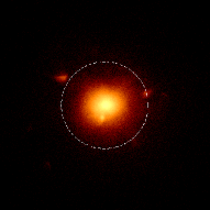
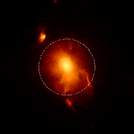
Only 1 out of the 65 clusters appears very relaxed according to all the above criteria. If we relax the criteria to allow for the existence of small concentrated substructures that can be removed by the clump-removing method, then 3 more clusters can be classified as ‘very relaxed’. We construct larger sub-samples of clusters by further relaxing the criteria: a ‘rather relaxed’ sample of 14 clusters which have no or only slight disturbances in the core region and the global ICM, and contain no or only small concentrated substructures within and around $r_{\rm 500}$; and a ‘less disturbed’ sample of 32 clusters (including the ‘rather relaxed’ clusters) which have single, distinguished cluster core and no significant substructure between cluster core region and $r_{\rm 500}$. Fig. 2 shows mock Chandra X-ray images of representative clusters of these samples.

2.5 Results

Figure 3: HSE mass biases at $r_{\rm 500}$ (upper panel) and their correction with the simulated non-thermal pressure (middle panel) and the modeled non-thermal pressure (lower panel) for the ‘rather relaxed’ clusters. The 14 clusters are ordered by their degree of relaxation, ranging from very relaxed on the left (number 1) to slightly disturbed on the right (number 14). The masses are estimated using profiles between 0.1 and 1.5 $r_{\rm 500}^{\rm true}$ with four methods mentioned in the text: a spline smoothing method (S) and three parametrized model fitting methods (NG, VV and VG). The averaged mass biases for the sample before and after correction are given in Fig. 5 and Table 1.

Figure 4: Effect of fitting range on the HSE mass bias. HSE mass biases at $r_{\rm 500}$ of the ‘rather relaxed’ 14 clusters estimated using the parametrized fitting method ‘NG’ are shown.

Figure 5: Averaged HSE (open markers) and corrected (filled markers) mass biases at $r_{\rm 500}$ and their scatter for cluster samples of different relaxation states: top 14 (‘rather relaxed’) and 32 (‘less disturbed’), and the full mass limited 65 clusters (‘all’). The fitting / smoothing method is indicated by the label on the x-axis, with symbols identical to that in Fig. 3. Fitting methods are performed using profiles on two different radial ranges: [0.1, 1] $r_{\rm 500}^{\rm true}$ (circles) and [0.1, 1.5] $r_{\rm 500}^{\rm true}$ (squares). The numerical values are given in Table 1.

Table 1: Numerical values of Bias $\pm$ Scatter in mass estimations with the fitting method ‘NG’ shown by the red symbols and error bars in Fig. 5. The values for the progenitors at $z=0.6$ are also shown in the last column.

	fitting range	rather relaxed (14/65)	less disturbed (32/65)	mass-limited (65/65)	progenitors at z=0.6 (65/65)
$\ln(M_{\rm HSE}/M_{\rm true})$	[0.1, 1] $r_{\rm{500}}^{\rm true}$	$-0.09\pm 0.14$	$-0.14\pm 0.23$	$-0.23\pm 0.31$	$-0.24\pm 0.26$
	[0.1, 1.5] $r_{\rm{500}}^{\rm true}$	$-0.16\pm 0.08$	$-0.21\pm 0.14$	$-0.24\pm 0.15$	$-0.26\pm 0.15$
$\ln(M_{\rm corr}/M_{\rm true})$	[0.1, 1] $r_{\rm{500}}^{\rm true}$	$-0.01\pm 0.18$	$-0.02\pm 0.27$	$-0.04\pm 0.32$	$-0.07\pm 0.28$
	[0.1, 1.5] $r_{\rm{500}}^{\rm true}$	$-0.07\pm 0.11$	$-0.04\pm 0.17$	$-0.03\pm 0.20$	$-0.05\pm 0.18$

2.5.1 Influence of mass estimation methods on the HSE mass bias

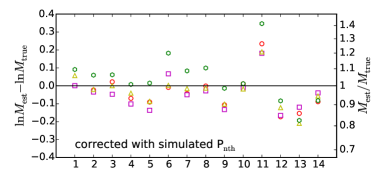
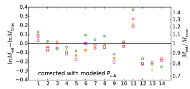
In the upper panel of Fig. 3 we show the HSE mass biases of the 14 ‘rather relaxed’ clusters. Given the same input gas density and pressure profiles, the HSE masses estimated using different approaches (Sect. 2.2 and 2.3) vary at the level of 5-10% for all 14 clusters. None of the four approaches systematically give significantly smaller or larger HSE mass biases, suggesting that they are comparable in a statistical sense. Even for the few most relaxed clusters (cluster number 1-4), there exist 5-10% HSE mass biases, confirming the need for non-thermal pressure correction even for the relaxed cluster sample typically used for calibrating the scaling relation.

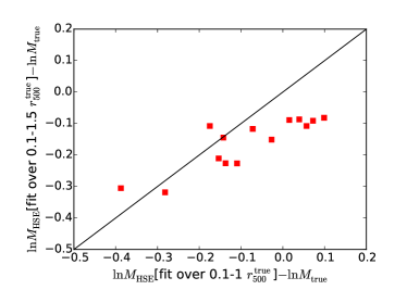
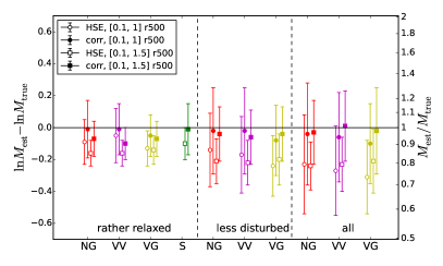
Fitting to different radial ranges also introduces 5-10% differences in the HSE mass estimates (Fig. 4). Fitting to larger radii more likely gives larger HSE mass biases. This is because the increase of non-thermal pressure with radius causes additional steepening of $P_{\rm th}$ compared to $P_{\rm tot}$, so when data from larger radii are considered in the fit, larger HSE mass biases are favored given the limited flexibility of any fitting formula. Being a weak effect, this systematic trend is visible only for relatively relaxed clusters (Fig. 5).

2.5.2 Correction for the HSE mass bias

How well can we correct for the HSE mass bias with the SK14 analytical model for non-thermal pressure? The lower panel of Fig. 3 shows the corrected masses for the ‘rather relaxed’ clusters. The correction for individual clusters is not perfect, which is also the case if we correct for the masses using the simulated $P_{\rm nth}$ (middle panel). The imperfection of HSE mass correction with simulated $P_{\rm nth}$ is also noticed in Nelson et al. (2014). This imperfection is most likely due to asphericity and the small scale structure of the ICM as well as residual accelerations which also breaks the HSE assumption (Lau, Nagai & Nelson, 2013). However, the average HSE mass bias for the 14 clusters is greatly reduced after correction, both with simulated and modeled $P_{\rm nth}$, irrespective of which smoothing/fitting method is used. This is more apparent from Fig. 5, where we show the averaged HSE (open markers) and corrected (filled markers) mass biases and their scatter. Remarkably, for the ‘less disturbed’ and even the full mass-limited sample, both at z=0 (5th column of Table 1) and a high redshift of z=0.6 (6th column), the biases are successfully reduced to be well below 10% irrespective of the smoothing/fitting method or the fitting range (Fig. 5; Table 1). This suggests that, the HSE mass biases related to non-thermal pressure can be corrected robustly for the sample average with the SK14 model for clusters in a wide range of dynamical states and redshifts, which will be obtained with combined X-ray surface brightness and SZ observations.

3 Conclusions and Discussions

There is no universal value for the HSE mass bias due to non-thermal pressure. Not only does it depend on masses, radii, and redshifts (SK14), but it also depends on the particular fitting or smoothing method used to compute the HSE mass from the observed profiles, as well as on the radial range of the data used for the fitting. Thus, to evaluate how much non-thermal pressure contributes to the ‘Planck CMB-cluster tension’, the particular method used by the Planck team needs to be tested e.g. on simulated cluster samples.

Non-thermal pressure biases the masses, hence the mass-observable scaling relations, even for the most relaxed clusters in the mass-limited sample in the simulation. This poses a challenge to the commonly adopted approach of calibrating the scaling relation on a sample of relaxed clusters and applying it to the full cluster sample at all dynamical states. Correction for non-thermal pressure is needed for the calibration of the scaling relation on relaxed clusters too because non-thermal motions are continuously sourced by the mass accretion and are never fully thermalized, especially at the cluster outskirts.

The SK14 model is able to correct the non-thermal pressure biases in the mass-limited sample and its dynamically more relaxed subsamples, irrespective of the dynamical state, the smoothing or the fitting method used for the mass estimation, or the radial range of data used in the fitting. Aided by this correction, the HSE mass estimate may no longer be limited by non-thermal pressure or dynamical state of the cluster. This opens up a possibility for more accurate cluster mass determinations using combined X-ray surface brightness and SZ observations. Compared to cluster masses estimated using weak gravitational lensing, the bias-corrected HSE masses are more precise, i.e. have smaller statistical uncertainties. Nevertheless, it will be important to check the consistency of both methods.

Gas motions in the ICM will be probed by the upcoming ASTRO-H mission (Takahashi et al., 2012) through the shifts and broadening of the X-ray spectral lines (ZuHone, Markevitch & Zhuravleva, 2015; Ota, Nagai & Lau, 2015). However, the measurements will be limited to a small number of clusters and small radii ($r\lesssim r_{\rm 2500}$) where the random motions are mild. Although the measurements cannot be directly used to correct mass estimations at $r_{\rm 500}$, they will test our current understanding on the nature of gas motions in the ICM.

The necessary input of the SK14 model is the mass accretion history of clusters. Although not directly observable, the mass accretion history is known in a sample-averaged sense from dark matter-only cosmological simulations (e.g. Zhao et al., 2009), though its cosmology dependence awaits more detailed simulation studies. Our simple correction method reduces the mean of the mass biases but not yet the scatter, which means no advantage will be gained by correcting HSE mass biases for individual clusters at this stage. If the residual acceleration, asphericity and small scale structures of the ICM, which are the most likely sources of the scatter, are better understood in the future, then knowledge of non-thermal pressure in individual clusters will be very helpful in getting accurate individual masses. The mass accretion history and the non-thermal pressure for individual clusters may also be obtainable by exploiting the connection between the mass density profile and the mass accretion history (Ludlow et al., 2013; Diemer & Kravtsov, 2014). Namely, first compute a mass profile from a cluster without correcting for non-thermal pressure, and then compute the mass accretion history from the mass profile, compute non-thermal pressure, and recompute the mass profile. Then iterate until the mass profile converges. We leave this for future work.

Appendix A Velocity anisotropy

In the absence of streaming motions, the steady-state radial Jeans equation gives (see e.g. Lau, Nagai & Nelson, 2013)

$$\frac{GM(<r)}{r^{2}}=-\frac{1}{\rho_{\rm gas}}\frac{\partial\left(P_{\rm th}+\rho_{\rm gas}\sigma^{2}_{r}\right)}{\partial r}-\frac{\left(2\sigma^{2}_{r}-\sigma^{2}_{t}\right)}{r}\,,$$ (10)

where $\sigma^{2}_{r}$ is the radial non-thermal velocity dispersion, and $\sigma^{2}_{t}=\sigma^{2}_{\theta\theta}+\sigma^{2}_{\phi\phi}$ is the tangential non-thermal velocity dispersion.

Let us define the velocity anisotropy parameter, $\beta$, as

$$\beta\equiv 1-\frac{\sigma^{2}_{t}}{2\sigma^{2}_{r}}\,.$$ (11)

This parameter vanishes for isotropic velocity distribution, and equation (10) reduces to equation (2) with $P_{\rm nth}=\rho_{\rm gas}\sigma_{\rm nth}^{2}$. Here, $\sigma^{2}_{\rm nth}\equiv(\sigma^{2}_{r}+\sigma^{2}_{t})/3$ is the averaged one-dimensional non-thermal velocity dispersion squared.

We calculate the influence of a non-zero anisotropy parameter on the HSE mass estimate. Inserting equation (11) into equation (10), we obtain

$$\begin{split}&M(<r)=-\frac{r^{2}}{G\rho_{\rm gas}}\frac{\partial P_{\rm th}}{\partial r}-\frac{3}{3-2\beta}\frac{r\sigma^{2}_{\rm nth}}{G}\times\\ &\left[\frac{\partial\ln\rho_{\rm gas}}{\partial\ln r}+\frac{\partial\ln\sigma^{2}_{\rm nth}}{\partial\ln r}-\frac{\partial\ln\left(3-2\beta\right)}{\partial\ln r}+2\beta\right]\,.\end{split}$$ (12)

When $\beta\neq 0$, the difference between the mass estimates without assuming $\beta=0$, $M_{\beta}$, and assuming $\beta=0$, $M_{\beta=0}$, is given by

$$\begin{split}&-\frac{G}{r\sigma^{2}_{\rm nth}}\left[{M_{\beta}(<r)-M_{\beta=0}(<r)}\right]=\frac{2\beta}{3-2\beta}\frac{\partial\ln\rho_{\rm gas}}{\partial\ln r}+\frac{6\beta}{3-2\beta}\\ &+\frac{2\beta}{3-2\beta}\frac{\partial\ln\sigma^{2}_{\rm nth}}{\partial\ln r}-\frac{3}{3-2\beta}\frac{\partial\ln\left(3-2\beta\right)}{\partial\ln r}\,.\end{split}$$ (13)

The first two terms on the r.h.s. dominate; however, they cancel when $\rho_{\rm gas}$ has a logarithmic slope of $-3$, which happens to coincide with the outer slope of an NFW profile. At $r_{\rm 500}$, $\rho_{\rm gas}$ typically has a slightly shallower logarithmic slope than $-3$, but still letting these terms cancel to a large extent. Therefore, the difference in mass corrections with and without including velocity anisotropy is expected to be smaller than the mass correction itself, which is

$$-\frac{G}{r\sigma^{2}_{\rm nth}}\left[M_{\rm corr}(<r)-M_{\rm HSE}(<r)\right]=\frac{\partial\ln\rho_{\rm gas}}{\partial\ln r}+\frac{\partial\ln\sigma^{2}_{\rm nth}}{\partial\ln r}\,.$$ (14)

Figure 6: Difference in the $M_{\rm corr}$ obtained by assuming and not assuming $\beta=0$ when correcting for non-thermal pressure is smaller than the correction itself, $M_{\rm true}-M_{\rm HSE}$, for the majority of clusters in the simulation. The color scale shows $\beta$: red for bigger $\beta$ and blue for smaller $\beta$. The stars show the subsample of relaxed clusters, while the circles show the rest. Only 10 out of 65 clusters show $|M_{\rm corr,\beta}-M_{\rm corr,\beta=0}|>M_{\rm true}-M_{\rm HSE}$.

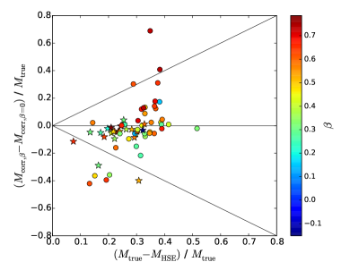In this Appendix, we use the cubic spline smoothing method to regularize the simulated cluster profiles in the radial range of [0.01, 3] $r_{\rm 500}^{\rm true}$. Fig. 6 shows that the difference between assuming and not assuming $\beta=0$ is indeed smaller than the correction itself, i.e., $M_{\rm true}-M_{\rm HSE}$, for the majority of clusters. Even in the cases where the difference is significant, the mass estimated by taking into account the velocity anisotropy is not always closer to the true mass. Thus including velocity anisotropy does not give significantly improved results. This, together with that $\beta(r)$ is not observable, makes us conclude that the simple mass correction given in equation (2) would already suffice.

Appendix B From non-thermal pressure to mass bias

Figure 7: Correlation between non-thermal pressure and the HSE mass bias at $r_{500}$. The open and filled symbols show $M_{\rm HSE}/M_{\rm true}$ from the ‘NG’ parametric fitting and the cubic spline smoothing methods, respectively, as a function of the non-thermal fraction, $f_{\rm nth}$, at $r_{500}$. The stars show the subsample of relaxed clusters, while the triangles show the rest. The dashed and solid lines show the slopes of $-1$ and $-2.5$ to guide the eye.

In this Appendix, we show how an error on the pressure profile propagates to an error on the mass. According to equation (4), an error on the pressure gradient will lead to an error on $\mathbf{\Delta}(r)$ as $\delta\ln\mathbf{\Delta}=-\delta\ln(\partial P/\partial r)$. Since the error on the estimation of $r_{\Delta}$ is related to the error on the $\mathbf{\Delta}(r)$ profile through the chain rule $\delta\ln(r)=\delta\ln\mathbf{\Delta}(r)\;(\partial\ln\mathbf{\Delta}/\partial\ln r)^{-1}$, the cluster mass will be miss-estimated by

$$\delta\ln(M_{\Delta})=3\delta\ln(r_{\Delta})=-3\delta\ln\left(\frac{\partial P}{\partial r}\right)\left(\frac{\partial\ln\mathbf{\Delta}(r)}{\partial\ln r}\right)^{-1}\bigg{|}_{r_{\Delta}}\,.$$ (15)

The slope of $\mathbf{\Delta}(r)$ is approximately $-2$ ($\pm 0.2$) at a radius of $r_{\rm 500}$ for an NFW mass density profile with a concentration parameter typical of clusters. Hence, $\delta\ln(M_{\Delta})\approx 3\delta\ln\left(\partial P/\partial r\right)/2$.

The relation between the change in the pressure gradient $\delta\ln\left(\partial P/\partial r\right)$ and the non-thermal fraction $f_{\rm nth}$ is:

$$\begin{split}&\delta\ln\left(\frac{\partial P}{\partial r}\right)\equiv\ln\left(\frac{\partial P_{\rm th}}{\partial r}\right)-\ln\left(\frac{\partial P_{\rm tot}}{\partial r}\right)\\ =&\ln(1-f_{\rm nth})+\ln\left[1+\left(\frac{\partial\ln P_{\rm tot}}{\partial\ln r}\right)^{-1}\frac{\partial\ln(1-f_{\rm nth})}{\partial\ln r}\right]\,.\end{split}$$ (16)

In the limit that $f_{\rm nth}$ is small and constant with radius, the relation is linear: $\delta\ln(M_{\Delta})\approx-3f_{\rm nth}/2$. In practice, $f_{\rm nth}$ is radial dependent (Shi & Komatsu, 2014), and this relation also depends on the method used in regularizing the input cluster profiles. We show in Fig. 7 that $|\delta\ln(M_{\Delta})|$ estimated with both the ‘NG’ fitting and the cubic spline smoothing methods correlate positively with $f_{\rm nth}$, and the fitting method yields a significantly larger HSE mass bias since we fit out to a large radius of 3$r_{\rm 500}^{\rm true}$ here.

If the HSE mass estimation is performed at the true $r_{\Delta}$ (as e.g. in Sect. 6 of SK14), the mass bias is $\delta\ln(M_{\Delta})=\delta\ln\left(\partial P/\partial r\right)$, i.e., about 2/3 of the above value.

Appendix C Comparison of dynamical state classifications

Figure 8: Distributions of Mantz et al. (2015) morphological values for the simulated mass-limited cluster sample at $z=0$. The s-p-a cuts defining the relaxed sub-sample given in Mantz et al. (2015) are shown as dashed lines. In comparison, galaxy clusters classified into different dynamical state categories using method given in this paper are indicated by different markers: ‘very relaxed’ (green star), ‘rather relaxed’ (blue circles and the green star), ‘less disturbed’ (magenta triangles, blue circles and the green star), and ‘disturbed’ (red crosses).

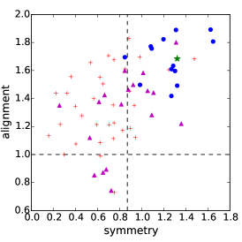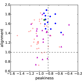
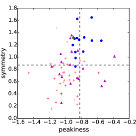
Recently, Mantz et al. (2015) developed an automatic method for classifying the relaxation state of galaxy clusters. Their classification is based on the symmetry (‘s’), peakiness (‘p’), and alignment (‘a’) of their X-ray morphologies, similar to the factors we consider for our classification (Sect. 2.4). Here we compare the two classification methods on our simulated mass-limited cluster sample at $z=0$ using mock X-ray images with 100 kilo-seconds exposure time (Fig. 8).

In Mantz et al. (2015) classification, a cluster is categorized as relaxed when a s-p-a criterion of $s>0.87$, $p>-0.82$, and $a>1.00$ (dashed lines in Fig. 8) is satisfied in more than 50% of the cases of its bootstrap analysis. This results in a relaxed cluster fraction of about 16%, slightly smaller than the fraction (21%) of our ‘rather relaxed’ clusters (blue circles and the green star in Mantz et al. (2015)). In general, more relaxed clusters in our simulated sample according to our classification also have higher $s$-$p$-$a$ values, showing overall agreement of the two classification methods. The specific distribution of $s$-$p$-$a$ values of our simulated cluster sample is slightly shifted compared to the distribution of morphological values of the Chandra sample (Fig. 8, Mantz et al. (2015)): our simulated clusters have systematically higher alignment values, and lower peakiness values. This is likely due to the inability of non-radiative simulations in reproducing the observed properties of the cluster core. After taking the corresponding shifted $s$-$p$-$a$ criterion into consideration, the distribution of $s$-$p$-$a$ values of our ‘rather relaxed’ clusters aligns rather well with that of the relaxed clusters as classified with Mantz et al. (2015) method.

References

- Allen, Evrard & Mantz (2011) Allen S. W., Evrard A. E., Mantz A. B., 2011, Ann.Rev.Astron.Astrophys., 49, 409
- Andersson et al. (2011) Andersson K. et al., 2011, ApJ, 738, 48
- Arnaud et al. (2010) Arnaud M., Pratt G. W., Piffaretti R., Böhringer H., Croston J. H., Pointecouteau E., 2010, A&A, 517, A92
- Battaglia et al. (2012) Battaglia N., Bond J. R., Pfrommer C., Sievers J. L., 2012, ApJ, 758, 74
- Bender et al. (2014) Bender A. N. et al., 2014, arXiv: 1404.7103
- Cavaliere & Fusco-Femiano (1978) Cavaliere A., Fusco-Femiano R., 1978, A&A, 70, 677
- Diemer & Kravtsov (2014) Diemer B., Kravtsov A. V., 2014, ApJ, 789, 1
- Dierckx (1993) Dierckx P., 1993, Curve and surface fitting with splines. Oxford: Clarendon
- Donahue et al. (2014) Donahue M. et al., 2014, ApJ, 794, 136
- Giodini et al. (2013) Giodini S., Lovisari L., Pointecouteau E., Ettori S., Reiprich T. H., Hoekstra H., 2013, Space Science Reviews, 177, 247
- Israel et al. (2015) Israel H., Schellenberger G., Nevalainen J., Massey R., Reiprich T. H., 2015, MNRAS, 448, 814
- Kay et al. (2004) Kay S. T., Thomas P. A., Jenkins A., Pearce F. R., 2004, MNRAS, 355, 1091
- Kravtsov, Vikhlinin & Nagai (2006) Kravtsov A. V., Vikhlinin A., Nagai D., 2006, ApJ, 650, 128
- Lau, Kravtsov & Nagai (2009) Lau E. T., Kravtsov A. V., Nagai D., 2009, ApJ, 705, 1129
- Lau, Nagai & Nelson (2013) Lau E. T., Nagai D., Nelson K., 2013, ApJ, 777, 151
- Leistedt, Peiris & Verde (2014) Leistedt B., Peiris H. V., Verde L., 2014, Physical Review Letters, 113, 041301
- Ludlow et al. (2013) Ludlow A. D. et al., 2013, MNRAS, 432, 1103
- Mantz et al. (2015) Mantz A. B., Allen S. W., Morris R. G., Schmidt R. W., von der Linden A., Urban O., 2015, MNRAS, 449, 199
- Meneghetti et al. (2010) Meneghetti M., Rasia E., Merten J., Bellagamba F., Ettori S., Mazzotta P., Dolag K., Marri S., 2010, A&A, 514, A93
- Nagai, Kravtsov & Vikhlinin (2007) Nagai D., Kravtsov A. V., Vikhlinin A., 2007, ApJ, 668, 1
- Nagai et al. (2013) Nagai D., Lau E. T., Avestruz C., Nelson K., Rudd D. H., 2013, ApJ, 777, 137
- Nagai, Vikhlinin & Kravtsov (2007) Nagai D., Vikhlinin A., Kravtsov A. V., 2007, ApJ, 655, 98
- Navarro, Frenk & White (1996) Navarro J. F., Frenk C. S., White S. D. M., 1996, ApJ, 462, 563
- Nelson, Lau & Nagai (2014) Nelson K., Lau E. T., Nagai D., 2014, ApJ, 792, 25
- Nelson et al. (2014) Nelson K., Lau E. T., Nagai D., Rudd D. H., Yu L., 2014, ApJ, 782, 107
- Nelson et al. (2012) Nelson K., Rudd D. H., Shaw L., Nagai D., 2012, ApJ, 751, 121
- Ota, Nagai & Lau (2015) Ota N., Nagai D., Lau E. T., 2015, arXiv: 1507.02730
- Piffaretti & Valdarnini (2008) Piffaretti R., Valdarnini R., 2008, A&A, 491, 71
- Planck Collaboration V. (2013) Planck Collaboration V., 2013, A&A, 550, A131
- Planck Collaboration XX. (2014) Planck Collaboration XX., 2014, A&A, 571, A20
- Planck Collaboration XXIV. (2015) Planck Collaboration XXIV., 2015, arXiv: 1502.01597
- Pointecouteau, Arnaud & Pratt (2005) Pointecouteau E., Arnaud M., Pratt G. W., 2005, A&A, 435, 1
- Rasia et al. (2006) Rasia E. et al., 2006, MNRAS, 369, 2013
- Rasia et al. (2012) Rasia E. et al., 2012, New Journal of Physics, 14, 055018
- Reiprich & Böhringer (2002) Reiprich T. H., Böhringer H., 2002, ApJ, 567, 716
- Schmidt & Allen (2007) Schmidt R. W., Allen S. W., 2007, MNRAS, 379, 209
- Shi et al. (2015) Shi X., Komatsu E., Nelson K., Nagai D. S., 2015, MNRAS, 448, 1020
- Shi & Komatsu (2014) Shi X., Komatsu E. S., 2014, MNRAS, 442, 521
- Sunyaev & Zeldovich (1970) Sunyaev R. A., Zeldovich Y. B., 1970, Comments on Astrophysics and Space Physics, 2, 66
- Sunyaev & Zeldovich (1972) Sunyaev R. A., Zeldovich Y. B., 1972, Comments on Astrophysics and Space Physics, 4, 173
- Takahashi et al. (2012) Takahashi T. et al., 2012, in Society of Photo-Optical Instrumentation Engineers (SPIE) Conference Series, Vol. 8443, Society of Photo-Optical Instrumentation Engineers (SPIE) Conference Series
- Vikhlinin et al. (2009) Vikhlinin A. et al., 2009, ApJ, 692, 1033
- Vikhlinin et al. (2006) Vikhlinin A., Kravtsov A., Forman W., Jones C., Markevitch M., Murray S. S., Van Speybroeck L., 2006, ApJ, 640, 691
- von der Linden et al. (2014) von der Linden A. et al., 2014, MNRAS, 443, 1973
- Zhao et al. (2009) Zhao D. H., Jing Y. P., Mo H. J., Börner G., 2009, ApJ, 707, 354
- Zhao (1996) Zhao H., 1996, MNRAS, 278, 488
- Zhuravleva et al. (2013) Zhuravleva I., Churazov E., Kravtsov A., Lau E. T., Nagai D., Sunyaev R., 2013, MNRAS, 428, 3274
- ZuHone, Markevitch & Zhuravleva (2015) ZuHone J., Markevitch M., Zhuravleva I., 2015, arXiv: 1505.07848