Kevin Buchin, Tim Ophelders and Bettina Speckmann
Computing the Similarity Between Moving Curves
Abstract.
In this paper we study similarity measures for moving curves which can, for example, model changing coastlines or retreating glacier termini. Points on a moving curve have two parameters, namely the position along the curve as well as time. We therefore focus on similarity measures for surfaces, specifically the Fréchet distance between surfaces. While the Fréchet distance between surfaces is not even known to be computable, we show for variants arising in the context of moving curves that they are polynomial-time solvable or NP-complete depending on the restrictions imposed on how the moving curves are matched. We achieve the polynomial-time solutions by a novel approach for computing a surface in the so-called free-space diagram based on max-flow min-cut duality.
Key words and phrases:
Fréchet distance, distance between surfaces, complex moving objects, moving curves1991 Mathematics Subject Classification:
I.3.5 Computational Geometry and Object Modeling1. Introduction
Over the past years the availability of devices that can be used to track moving objects has increased dramatically, leading to an explosive growth in movement data. Naturally the goal is not only to track objects but also to extract information from the resulting data. Consequently recent years have seen a significant increase in the development of methods extracting knowledge from moving object data.
Tracking an object gives rise to data describing its movement. Often the scale at which the tracking takes place is such that the tracked objects can be viewed as point objects. Cars driving on a highway, birds foraging for food, or humans walking in a pedestrian zone: for many analysis tasks it is sufficient to consider objects as moving points. Hence the most common data sets used in movement data processing are so-called trajectories: sequences of time-stamped points.
However, not all moving objects can be reasonably represented as points. A hurricane can be represented by the position of its eye, but a more accurate description is as a 2-dimensional region which represents the hurricane’s extent. When studying shifting coastlines, reducing the coastline to a point is obviously unwanted: one is actually interested in how the whole coast line moves and changes shape over time. The same holds true when studying the terminus of a glacier. In such cases, the moving object is best represented as a polyline rather than by a single point. In this paper we hence go beyond the basic setting of moving point objects and study moving complex, non-point objects. Specifically, we focus on similarity measures for moving curves, based on the Fréchet distance.
Definitions and Notation. The Fréchet distance is a well-studied distance measure for shapes, and is commonly used to determine the similarity between two curves and . A natural generalization to more complex shapes uses the definition of Equation 1 where the shapes and have type .
| (1) |

Here, is a norm such as the Euclidean norm () or the Manhattan norm (). The matching ranges over orientation-preserving homeomorphisms (possibly with additional constraints) between the parameter spaces of the shapes compared; as such, it defines a correspondence between the points of the compared shapes. A matching between surfaces with parameters and is illustrated in Figure 1. Given one such matching we obtain a distance between and by taking the largest distance between any two corresponding points of and . The Fréchet distance is the infimum of these distances taken over all possible matchings. For moving points or static curves, we have as parameter space and for moving curves or static surfaces, we have . We can define various similarity measures between shapes by imposing further restrictions on .
In practice a curve is generally represented by a sequence of points. Assuming a linear interpolation between consecutive points, this results in a polyline with segments. Analogously, a moving curve is a sequence of polylines, each of segments. We also interpolate the polylines linearly, yielding a bilinear interpolation, or a quadrilateral mesh of quadrilaterals.
Related Work. The Fréchet distance or related measures are frequently used to evaluate the similarity between point trajectories [8, 7, 13]. The Fréchet distance is also used to match point trajectories to a street network [2, 5]. The Fréchet distance between polygonal curves can be computed in near-quadratic time [3, 6, 9, 18], and approximation algorithms [4, 16] have been studied.
The natural generalization to moving (parameterized) curves is to interpret the curves as surfaces parameterized over time and over the curve parameter. The Fréchet distance between surfaces is NP-hard [17], even for terrains [10]. In terms of positive algorithmic results for general surfaces the Fréchet distance is only known to be semi-computable [1, 12]. Polynomial-time algorithms have been given for the so called weak Fréchet distance [1] and for the Fréchet distance between simple polygons [11] and so called folded polygons [15].
When interpreting moving curves as surfaces it is important to take the different roles of the two parameters into account: the first is inherently linked to time and the other to space. This naturally leads to restricted versions of the Fréchet distance of surfaces. For curves, restricted versions of the Fréchet distance were considered [7, 19]. For surfaces we are not aware of similar results.
1.1. Results
We refine the Fréchet distance between surfaces to meaningfully compare moving curves. To do so, we restrict matchings to be one of several suitable classes. Representative matchings for the considered classes together with the running times of our results are illustrated in Figure 2.
| Identity |
| Synchronous Constant |
| Synchronous Dynamic |
| Asynchronous Constant |
| NP-complete |
| Asynchronous Dynamic |
| NP-hard |
| Orientation-Preserving |
| NP-hard |
The simplest class of matchings consists of a single predefined identity matching . Hence, to compute the identity Fréchet distance, we need only determine a pair of matched points that are furthest apart. It turns out that one of the points of a furthest pair is a vertex of a moving curve (i.e. quadrilateral mesh), allowing computation in time, see Section 2.
We discuss the synchronous constant Fréchet distance in Section 3. Here we assume that the matching of timestamps is known in advance, and the matching of positions is the same for each timestamp, so it remains constant. Our algorithm computes the positional matching minimizing the Fréchet distance.
The synchronous dynamic Fréchet distance considered in Section 4 also assumes a predefined matching of timestamps, but does not have the constraint of the synchronous constant class that the matching of positions remains constant over time. Instead, the positional matching may change continuously over time.
Finally, in Section 5, we consider several cases where neither positional nor temporal matchings are predefined. The three considered cases are the asynchronous constant, asynchronous dynamic, and orientation-preserving Fréchet distance. The asynchronous constant class of matchings consists of a constant (but not predefined) matching of positions, as well as timestamps whereas in the asynchronous dynamic class of matchings, the positional matching may change continuously. In the orientation-preserving class, matchings range over orientation preserving homeomorphisms between parameter spaces, given that the corners of the parameter spaces are aligned.
The last three classes are quite complex, and we give constructions proving that approximating the Fréchet distance within a factor is NP-hard under these classes. For the asynchronous constant and asynchronous dynamic classes of matchings, this result holds even for moving curves embedded in whereas the result for the orientation-preserving case holds for embeddings in .
Although we do not discuss classes where positional matchings are known in advance, these symmetric variants can be obtained by interchanging the time and position parameters for the discussed classes. Deciding which variant is appropriate for comparing two moving curves depends largely on how the data is obtained, as well as the use case for the comparison. For instance, the synchronous constant variant may be used on a sequence of satellite images which have associated timestamps. The synchronous dynamic Fréchet distance is better suited for sensors with different sampling frequencies, placed on curve-like moving objects.
2. Identity Matchings
![[Uncaptioned image]](/html/1507.03819/assets/x8.png)
Suppose we are given a single predefined matching between the moving curves and . We can compute the Fréchet distance under this matching if we can find the corresponding points of and that are furthest apart, see Equation 2.
| (2) |
If and are both of size , then the identity matching allows us to simplify into where is again a quadrilateral mesh of size . The Fréchet distance for the identity matching depends only on the point on that is furthest from the origin. To see this, consider a single quadrilateral, the point furthest from the origin must be one its four corners since all points on the quadrilateral lie within the convex hull of its four corner points. Hence, it suffices to check only the distance to the origin for the vertices of , see Equation 3. The Fréchet distance under the identity matching can then be computed in time.
| (3) |
Meshes of different size can be compared after introducing dummy vertices, such that the meshes have equal dimensions and each vertex has an aligned vertex on the other mesh. For this, it is important to note that any quadrilateral can be subdivided into an equivalent mesh of four quadrilaterals with any point on the original quadrilateral as their shared corner.
To extend this further, consider the case where the matching is defined by two piecewise-linear functions and of and vertices. This allows comparing moving curves under predefined realigments of timestamps as well as positions. For such a matching, the surface is a quadrilateral mesh of vertices. We illustrate this in Figure 3 for and with vertices . In such case timestamps of are matched with timestamps of .

The same can be done given a piecewise-linear reparameterization of positions. As a result, the Fréchet distance under a predefined piecewise-linear reparameterization of timestamps and positions can be computed in time.
3. Synchronous Constant Matchings
![[Uncaptioned image]](/html/1507.03819/assets/x10.png)
In this section, we consider the class of synchronous constant matchings where the matching assumes no realignments of time and a constant reparameterization111We make slight abuse of notation: we allow to be drawn from the closure of the space of matchings. As a consequence, is not an actual function since some can be matched to multiple (but connected) values. of positions. Thus, the goal is to find a continuous nondecreasing surjection on , such that the Fréchet distance is minimized.
Before we present the algorithm to find synchronous constant matchings, we refer to an existing algorithm [3] that computes the Fréchet distance between static curves. This classic algorithm makes use of a data structure called the -freespace diagram, which is the set of parameter pairs for which the represented points are at most apart. A freespace diagram for two static curves is illustrated in Figure 4.
The matching between the parameter spaces of static curves and can be embedded as a bimonotone path in the freespace. Therefore, the Fréchet distance is at most if and only if there exists a bimonotone path from the bottom-left to the top-right corner of the -freespace. Using freespace diagrams, the decision problem for static curves can be solved in time.
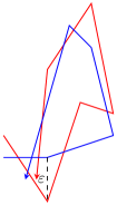
We extend this approach to compute matchings between moving curves. For this, consider the 3D freespace defined by Equation 4. Since any synchronous constant matching is defined by a bimonotone path , the matching is embedded in the freespace diagram as the surface . Such a matching yields a Fréchet distance of at most if and only if . The 3D freespace consists of cells for .
| (4) |
We can simplify the three-dimensional freespace () into a two-dimensional one () with
| (5) |
and find the path defining in it. To simplify Equation 5 we prove the following lemma.
Lemma 1.
A cell of the freespace has a convex intersection with any line parallel to the -plane or the -axis.
Proof.
Each cell in the freespace is the freespace induced by a pair of quadrilaterals, so consider two quadrilaterals and . These quadrilaterals are bilinear interpolations between four corner points. Hence, is an affine map for each fixed . Likewise, is an affine map for each fixed pair . Because the preimage of a convex norm ball under an affine map is convex, the intersection of a freespace cell with lines parallel to the -axis or the -plane forms a convex set. ∎
Lemma 2.
.
Proof.
By Lemma 1, the intersection of a cell of with a line parallel to the -axis is convex. Hence, if a point , then either or . Therefore the internal structure of freespace cells can safely be ignored. ∎
We denote the cells of the 2D freespace by where .
Lemma 3.
Every cell in the 2D freespace is convex.
Proof.
By Lemma 1, each cell is the intersection of convex sets, so each is convex. ∎
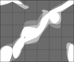
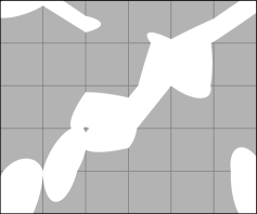
Figure 5 illustrates (in white) what the 2D freespace might look like for two moving curves. As before, any smaller value of would disconnect the bottom-left from the top-right corner. For a given , for each of the cells, the boundary intervals can be computed in time. Therefore, finding an -monotone path takes time, solving the decision problem for the Fréchet distance under synchronous constant matchings in time.
3.1. Parametric Search
To compute the exact Fréchet distance efficiently, we use the decision problem in a parametric search for the minimum admitting a matching. When increasing starting from , there are three types of critical values of for which a passage might open in the freespace:
-
a)
The minimal with and .
-
b)
One of the four boundaries of a cell becomes nonempty.
-
c)
The lower (or left) endpoint on the boundary of cell aligns with the upper (or right) endpoint on the boundary of (or ).
Note that all critical values occur when two endpoints align (or an endpoint aligns with a gridpoint). For each of the layers defining , we use a function in to represent the - or -position of such endpoint (or gridpoint). This amounts to a total of functions, and each critical value occurs when two of them intersect. Since the intersections between any pair of these functions can be computed in constant time, we can apply a parametric search [20].
We use Cole’s variant [14] of the parametric search to find the desired critical value in time. Here is the number of functions to which the parametric search is applied and is the running time for the decision problem. We obtain the running time of Theorem 4.
Theorem 4.
The synchronous constant Fréchet distance between quadrilateral meshes can be computed in time.
Remark.
To compare quadrilateral meshes under a piecewise linear realignment timestamps, we can subdivide the quadrilateral meshes as explained in Section 2. Although for simplicity we have assumed that the meshes are of equal size, when computing the Fréchet distance between meshes of different sizes, and , the 2D freespace has only cells. Thus the decision problem is solved in time and the exact computation takes time.
Remark.
If the inputs of the algorithm are two sequences of curves without predefined interpolations to obtain quadrilateral meshes, we can still measure their Fréchet distance for the optimal (but unknown) linear interpolation. Due to the convexity of freespace cells, the Fréchet distance is the minimum Fréchet distance between two curves and , which can be computed in time by running the original algorithm times.
4. Synchronous Dynamic Matchings
![[Uncaptioned image]](/html/1507.03819/assets/x14.png)
Synchronous dynamic matchings align timestamps under the identity matching, but the matching of positions may change continuously over time. Specifically, the matching is defined as . Here, is continuous, and for any the matching between the two curves at that time is a nondecreasing surjection.
4.1. Freespace Partitions in 2D
Recall that the freespace diagram is the set pairs of points that are within distance of each other.
If and are curves with parameter space , then their freespace diagram is two-dimensional, and the Fréchet distance is the minimum value of for which an -monotone path (representing ) from to through the freespace exists.
We use a variant of the max-flow min-cut duality to determine whether a matching through the freespace exists. Before we present the 3D variant for moving curves with synchronized timestamps, we illustrate the idea in the fictional 2D freespace of Figure 6.
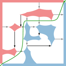
Here, any matching—such as the green path—must be an - and -monotone path from the bottom left to the top right corner and this matching must avoid all obstacles (i.e. all points not in ). Therefore each such matching divides the obstacles in two sets: those above, and those below the matching.
Suppose we now draw a directed edge from an obstacle to an obstacle if and only if any matching that goes over must necessarily go over . The key observation is that a matching exists unless such edges can form a path from the lower-right boundary to the upper-left boundary of the freespace. In the example, a few trivial edges are drawn in black and gray. If all obstacles were slightly larger, an edge could connect a blue obstacle with a red obstacle, connecting the two boundaries by the edges drawn in black.
4.2. Freespace Partitions in 3D
In contrast to the 2D freespace where the matching is a path, matchings of the form form surfaces in the 3D freespace (see Equation 6). Such a surface again divides the obstacles in the freespace in two sets and can be punctured by a path connecting two boundaries. We formalize this concept for the 3D freespace and give an algorithm for deciding the existence of a matching.
| (6) |
For , the cell of the 3D freespace is the set . The property of Lemma 1 holds for all such cells.
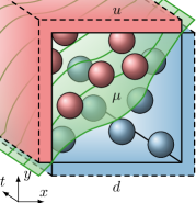
We divide the set of points not in into a set of so-called obstacles, such that each individual obstacle is a connected point set. Let be the open set of points representing the left and top boundary of . Symmetrically, let represent the bottom and right boundary, see Figure 7. Denote by the obstacles between the boundaries.
- :
-
with ;
- :
-
;
- :
-
.
Given a matching , let be the set of obstacles below it, then and . Here, we use axes and say that a point is below some other point if it has a smaller -coordinate. Because each obstacle is a connected set and cannot intersect obstacles, a single obstacle cannot lie on both sides of the same matching. Because all matchings have and , a matching exists if and only if .
We compute a relation of elementary dependencies between obstacles, such that its transitive closure has if and only if . Let if and only if is connected ( touches ) or there exists some point and with , and . We prove in Lemmas 5 and 6 that this choice of satisfies the required properties and in Theorem 7 that we can use the transitive closure of to solve the decision problem of the Fréchet distance.
Lemma 5.
If , then .
Proof.
Assume that , then either touches and no matching can separate them, or there exists some and with , . If there were some matching with , then for some . Similarly, if , then for some . We can further deduce from and monotonicity of that we can pick such that . However, this contradicts , so such a matching does not exist. Hence, whenever and therefore whenever . ∎
Lemma 6.
If , then .
Proof.
Suppose but not . Then no matching exists, and no path from to exists in the directed graph . Pick as the set of obstacles reachable from in , then does not contain . Pick the tightest matching such that lies below it, we define in terms of matchings in the plane at each timestamp .
Because , this defines a monotone path from to at each timestamp . Suppose that properly intersects some , such that some point of lies below . It follows from the definition of and that for some . However, such obstacle cannot exist because satisfies . As a result, no path intersects any obstacle and we can connect the paths to obtain a continuous matching without intersecting any obstacles. So does not intersect obstacles in , contradicting . ∎
Theorem 7.
The Fréchet distance is greater than if and only if for .
Proof.
We choose the set of obstacles such that and the relation is easily computable. Note that due to Lemma 1, each connected component contains a corner of a cell, so any cell in the freespace contains constantly many (up to eight) components of . Moreover, we can index each obstacle in by a grid point .
Let be the maximal connected subset of the cells adjacent to , such that contains . Now, the obstacle is not well-defined if , in which case we define to be an empty (dummy) obstacle. We have and we remark that obstacles are not necessarily disjoint.
Each of the obstacles is now defined by a constant number of vertices. We therefore assume that for each pair of obstacles , we can decide in constant time whether ; even though this decision procedure depends on the chosen distance metric. For each obstacle , there are obstacles for which , namely because if . Furthermore, and contribute to elements of the relation. Therefore we can compute the relation in time.
Testing whether is equivalent to testing whether a path from to exists in the directed graph , which can be decided using a depth first search. So we can solve the decision problem for the Fréchet distance in time. However, the relation may yield many unnecessary edges. In Section 4.4 we show that a smaller set of size with the same transitive closure is computable in time, so the decision algorithm takes only time.
4.3. Parametric Search
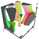
To give an idea of what the 3D freespace looks like, we have drawn the obstacles of the eight cells of the freespace between two quadrilateral meshes of size in Figure 8. Cells of the 3D freespace lie within cubes, having six faces and twelve edges. We call such edges -, - or -edges, depending on the axis to which they are parallel.
We are looking for the minimum value of for which a matching exists. When increasing the value of , the relation becomes sparser since obstacles shrink. Critical values of occur when changes. Due to Lemma 1, all critical values involve an edge or an -face or -face of a cell, but never the internal volume, so the following critical values cover all cases.
-
a)
The minimal such that and for all .
-
b)
An edge of becomes nonempty.
-
c)
Endpoints of -edges of and align in -coordinate, or endpoints of -edges of and align in -coordinate.
-
d)
Endpoints of a -edge of and a -edge of align in -coordinate.
-
e)
An obstacle in stops overlapping with an obstacle in or when projected along the - or -axis.
The endpoints involved in the critical values of type a), b), c) and d) can be captured in functions. We apply a parametric search for the minimum critical value of type a), b), c) or d) for which a matching exists. This takes time.
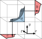
We illustrate the need for critical values of type e) in Figure 9, here obstacle overlaps with both obstacles and while the overlap in edges does not contribute to . It is unclear how critical values of type e) can be incorporated in the parametric search directly. Instead, we enumerate and sort the critical values of type e) in time. Using calls to the decision algorithm, we apply a binary search to find the minimum critical value of type e) for which a matching exists. Finding the critical value then takes time. The synchronous dynamic Fréchet distance is then the minimum of and . This results in the following running time.
Theorem 8.
The synchronous dynamic Fréchet distance can be computed in time.
Before stating the final running time, we present a faster algorithm for the decision algorithm.
4.4. A Faster Decision Algorithm
To speed up the decision procedure we distinguish the cases for which two obstacles may be related by , these cases correspond to the five types of critical values of Section 4.3. Critical values of type a) and b) depend on obstacles in single cells, so there are at most elements of arising from type a) and b). Critical values of type c) and e) arise from pairs of obstacles in cells in the same row or column, so there are at most of them. In fact, we can enumerate the edges of type a), b), c), and e) of in time. On the other hand, edges of type d) arise between two cells with the same value of , so there can be of them.
We compute a smaller directed graph with that has a path from to if and only if . Let be the vertices as before (we will include dummy obstacles for grid points in that lie in the freespace) and transfer the edges in except those of type d) to the smaller set of edges . We must still induce edges of type d) in , but instead of adding edges, we use only edges. The edges of type d) can actually be captured in the transitive closure of using only edges per obstacle in .
Using an edge from to and to , we construct a path from to any obstacle . The sole purpose of the dummy obstacles is to construct these paths effectively. For obstacles whose gridpoints have the same -coordinates, it then takes a total of edges to include the obstacles overlapping in -coordinate related by type d), this is valid because for non-dummy obstacles.
Denote by the edges of type d) of the form where , then the set of edges is the one we just constructed. Now it remains to induce paths with , that still overlap in -coordinates, i.e. the sets , , and . Denote by and the minimum and maximum -coordinate over points in an obstacle . For each obstacle, both the and the coordinates are an endpoint of a -edge in a cell defining the obstacle due to Lemma 1, and thus computable in constant time.
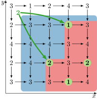
Our savings arise from the fact that induces a path from to if and with and , so we do not need an additional edge to induce a path to the latter obstacle. To avoid degenerate cases, we start by exhaustively enumerating edges of ( for which or in time so we need only consider edges with .
For these remaining cases, we have if and only if , and for positive . From this we can derive the edges of . Although for each , there may be obstacles such that with , the Pareto frontier of those obstacles contains only obstacles, see the grid of fictional values in Figure 10. In Section 4.5, we show how to find these Pareto frontiers in time per obstacle , using only preprocessing time for the complete freespace.
As a result, we can compute all edges of in time. By Theorem 9, the decision problem for the synchronous dynamic Fréchet distance is solvable in time.
Theorem 9.
The decision problem for the synchronous dynamic Fréchet distance is solvable in time.
Proof.
The edges of types other than d) are enumerated in time, and using constantly many Pareto frontier queries for each obstacle, edges of type d) in are computed in time. Given the set of edges, deciding whether a path between two vertices exists takes time. The transitive closure of equals , so a path from to exists in if and only if there was such a path in . Since we compute in time, the decision problem is solved in time. ∎
Corollary 10.
The synchronous dynamic Fréchet distance can be computed in time.
4.5. Pareto Frontier Queries
Suppose we are given a matrix with columns and rows, and we want to be efficiently query submatrices for the Pareto frontier of numbers that are at most a given threshold value, . A query specifies the threshold , and two coordinates and of the query rectangle . Let denote the coordinates of the query rectangle that must be dominated by the Pareto frontier . That is, if , then some with exists.
We preprocess each of the rows of in time by storing their cells as the leaves of an augmented binary tree, whose internal nodes store the minimum value over its subtrees. Then queries for the index of the leftmost element with value at most in a range of that row can be answered in time. We can compute by including for each row, the element with minimum -coordinate and value at most in the query range. So using queries, we compute a set of size in time, using preprocessing time for the matrix .
In this case, is not actually the Pareto frontier since some of its elements might be dominated by other elements. With a slight modification, we can make the actual Pareto frontier (of minimum size). If the query with range returns with for some row, then the query range for subsequent rows can be restricted to , so no unnecessary values are generated.
5. Hardness
![[Uncaptioned image]](/html/1507.03819/assets/x20.png)
![[Uncaptioned image]](/html/1507.03819/assets/x21.png)
We extend the synchronous constant and synchronous dynamic classes of matchings (of Sections 3 and 4) to asynchronous ones. For this, we allow realignments of timestamps, giving rise to the asynchronous constant and asynchronous dynamic classes of matchings. The asynchronous constant class ranges over matchings of the form where the and are matchings of positions and timestamps. The asynchronous dynamic class of matchings has the form for which the positional matching changes over time. We first prove that the asynchronous constant Fréchet distance is in NP.
Theorem 11.
Computing the Fréchet distance is in NP for the asynchronous constant class of matchings.
Proof.
Given any matching with a Fréchet distance of , we can derive—due to Lemma 1—a piecewise-linear matching in time, such that a matching with Fréchet distance at most exists. We can realign the quadrilateral meshes and under to obtain meshes and of polynomial size. Now the polynomial-time decision algorithm for synchronous constant matchings (see full paper) is applicable to and . ∎
Due to critical values of type e), it is unclear whether each asynchronous dynamic matching admits a piecewise-linear matching of polynomial size, which would mean that the asynchronous dynamic Fréchet distance is also in NP.
We show that computing the Fréchet distance is NP-hard for both classes by a reduction from 3-SAT. The idea behind the construction is illustrated in the two height maps of Figure 11. These represent quadrilateral meshes embedded in and correspond to a single clause of a 3-CNF formula of four variables.


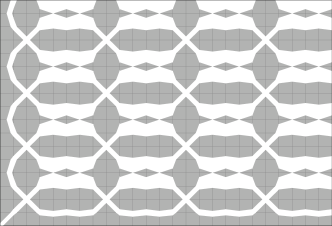
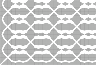
We distinguish valleys (dark), peaks (white on , yellow on ) and ridges (denoted , and ). An important observation is that in order to obtain a low Fréchet distance of , the -th valley of must be matched with the -th valley of . Moreover, each ridge must be matched with or and each peak of must be matched to a peak of . Note that even for asynchronous dynamic matchings, if is matched to , it cannot be matched to and vice-versa because the (red) valley separating and has distance from .
The aforementioned properties are reflected more clearly in the 2D freespace between the curves at aligned timestamps and . In Figure 12, we give two 2D slices (with and , respectively) of the 4D-freespace diagram with for the shown quadrilateral meshes. In this diagram with , only monotone paths exist (up to directed homotopy) whereas for there would be monotone paths (one for each assignment of variables). For , the peak of cannot be matched to at of , corresponding to an assignment of .
Consider a 3-CNF formula with variables and clauses, then and consist of clauses along the -axis and variables ( and ) along the -axis. The -th clause of is matched to the -th clause of due to the elevation pattern on the far left (). This means that the peaks of are matched with peaks of the same clause on and all these peaks have the same timestamp because is constant (independent of ).
For each clause, there are three rows (timestamps) of with peaks on the ridges. On each such timestamp, exactly one ridge (depending on the disjuncts of the clause) does not have a peak. Specifically, if a clause has or as its -th disjunct, then the -th row of that clause has no peak on ridge or , respectively. We use these properties in Theorem 14 where we prove that it is NP-hard to approximate the Fréchet distance within a factor .
Lemma 12.
The Fréchet distance between two such moving curves is at least if the corresponding 3-CNF formula is unsatisfiable.
Proof.
Consider a matching yielding a Fréchet distance smaller than given an unsatisfiable formula, then the peaks of (of the -th clause) are matched with peaks of (of a single row of the -th clause). Assign the value true to variable if ridge is matched with and false if it is matched with . Then for every clause with , there is a peak at , or for that clause. Such a matching cannot exist because then the 3-CNF formula would be satisfiable, so the Fréchet distance is at least . ∎
Lemma 13.
The Fréchet distance between two such moving curves is at most if the corresponding 3-CNF formula is satisfiable.
Proof.
Consider a satisfying assignment to the 3-CNF formula. Match with the center of or , if is false or true, respectively. For every clause, the timestamp with peaks of can be matched with a row of peaks on . As was already hinted at by Figure 11, the remaining parts of the curves can be matched with . Therefore this yields a Fréchet distance of at most . ∎
Theorem 14.
It is NP-hard to approximate the asynchronous constant or asynchronous dynamic Fréchet distance for moving curves in within a factor .
Proof.
5.1. Orientation-Preserving Homeomorphisms
![[Uncaptioned image]](/html/1507.03819/assets/x27.png)
Previous results [1, 10] have shown that computing the Fréchet distance between surfaces under orientation-preserving homeomorphisms is NP-hard for surfaces embedded in . We will refer to this variant as the orientation-preserving Fréchet distance. The prior results hold for triangular meshes, which are a degenerate case of quadrilateral meshes. Although the orientation-preserving Fréchet distance is upper-semicomputable, it is unknown whether it is computable at all. We consider the case where the corners of the meshes are matched with each other.
The prior NP-hardness constructions for the orientation-preserving Fréchet distance seem unnecessarily complex. Therefore we extend our results for the asynchronous dynamic Fréchet distance of Section 5 to obtain a new hardness construction for the orientation-preserving Fréchet distance for surfaces embedded in . Note that we cannot directly apply the previous construction because there was only a single matching of timestamps for asynchronous dynamic matchings. Thus, we do not preserve the property that for a clause, the timestamp with peaks of maps to a single timestamp of .
We prevent this by means of a second dimension in which we enforce that a row of peaks of maps to a single row of peaks of . In addition to the embedding in of Figure 11, which defines one coordinate for every point on a clause of a quadrilateral mesh, we define a second coordinate using Figure 13, yielding an embedding in .


Now, under the maximum norm (), a row of peaks of can only be matched to a single row of peaks on for . Conversely, we can still match the meshes of two satisfiable formulas with . Hence, Theorem 15 follows. This result extends to triangular meshes since all quadrilaterals lie in the plane, and can thus be represented by a pair of triangles. For norms other than the maximum norm, the problem is still NP-hard, but our bound on the approximation factor is smaller than .
Theorem 15.
Unless P=NP, no polynomial time algorithm can approximate the orientation-preserving Fréchet distance between two quadrilateral meshes embedded in under the maximum norm within a factor .
6. Conclusion
Based on the Fréchet distance, we presented several similarity measures between moving curves, together with efficient algorithms for computing some measures, while proving NP-hardness for computing others.
Although many algorithmic solutions to variants of the Fréchet distance between static curves also apply to the synchronous constant Fréchet distance, extending the synchronous dynamic class is more complex. For example, computing the synchronous dynamic Fréchet distance between moving closed curves (with a cylinder instead of square as parameter space) remains an open problem.
Finally, the performance of the algorithm for the synchronous dynamic Fréchet distance seems undesirably slow and we have not been able to prove tight lower bounds on this running time yet.
Acknowledgements. K. Buchin, T. Ophelders, and B. Speckmann are supported by the Netherlands Organisation for Scientific Research (NWO) under project no. 612.001.207 (K. Buchin) and no. 639.023.208 (T. Ophelders & B. Speckmann).
References
- [1] H. Alt and M. Buchin. Can we compute the similarity between surfaces? Discrete Comput. Geom., 43(1):78–99, 2010.
- [2] H. Alt, A. Efrat, G. Rote, and C. Wenk. Matching planar maps. In Proc. 14th Sympos. Discrete Algorithms, pages 589–598, 2003.
- [3] H. Alt and M. Godau. Computing the Fréchet distance between two polygonal curves. Intern. J. Comput. Geom. Appl., 5(01n02):75–91, 1995.
- [4] B. Aronov, S. Har-Peled, C. Knauer, Y. Wang, and C. Wenk. Fréchet Distances for Curves, Revisited. In Proc. 14th European Sympos. Algorithms, pages 52–63, 2006.
- [5] S. Brakatsoulas, D. Pfoser, R. Salas, and C. Wenk. On map-matching vehicle tracking data. In Proc. 31st Intern. Conf. VLDB, pages 853–864, 2005.
- [6] K. Bringmann. Why walking the dog takes time: Fréchet distance has no strongly subquadratic algorithms unless SETH fails. In Foundations of Computer Science, 2014, pages 661–670, 2014.
- [7] K. Buchin, M. Buchin, and J. Gudmundsson. Constrained free space diagrams: a tool for trajectory analysis. Intern. J. GIS, 24:1101–1125, 2010.
- [8] K. Buchin, M. Buchin, J. Gudmundsson, M. Löffler, and J. Luo. Detecting commuting patterns by clustering subtrajectories. Intern. J. Comput. Geom. Appl., 21(3):253–282, 2011.
- [9] K. Buchin, M. Buchin, W. Meulemans, and W. Mulzer. Four soviets walk the dog-with an application to Alt’s conjecture. In Proc. 25th Sympos. Discrete Algorithms, pages 1399–1413, 2014.
- [10] K. Buchin, M. Buchin, and A. Schulz. Fréchet distance of surfaces: Some simple hard cases. In Proc. 18th European Sympos. Algorithms, pages 63–74, 2010.
- [11] K. Buchin, M. Buchin, and C. Wenk. Computing the Fréchet distance between simple polygons. Comput. Geom. Theory Appl., 41(1–2):2–20, 2008.
- [12] M. Buchin. On the Computability of the Fréchet Distance Between Triangulated Surfaces. PhD thesis, Free University Berlin, Institute of Computer Science, 2007.
- [13] M. Buchin, S. Dodge, and B. Speckmann. Context-aware similarity of trajectories. In Proc. 6th Intern. Conf. GIS, pages 43–56, 2012.
- [14] R. Cole. Slowing down sorting networks to obtain faster sorting algorithms. J. ACM, 34(1):200–208, 1987.
- [15] A. F. Cook IV, A. Driemel, S. Har-Peled, J. Sherette, and C. Wenk. Computing the Fréchet distance between folded polygons. In Algorithms and Data Structures, pages 267–278, 2011.
- [16] A. Driemel, S. Har-Peled, and C. Wenk. Approximating the Fréchet distance for realistic curves in near linear time. Discrete Comput. Geom., 48(1):94–127, 2012.
- [17] M. Godau. On the complexity of measuring the similarity between geometric objects in higher dimensions. PhD thesis, Berlin, Freie Universität Berlin, Diss., 1998, 1999.
- [18] S. Har-Peled and B. Raichel. The Fréchet distance revisited and extended. ACM Transactions on Algorithms, 10(1):3, 2014.
- [19] A. Maheshwari, J.-R. Sack, K. Shahbaz, and H. Zarrabi-Zadeh. Fréchet distance with speed limits. Comput. Geom. Theory Appl., 44(2):110–120, 2011.
- [20] N. Megiddo. Applying parallel computation algorithms in the design of serial algorithms. J. ACM, 30(4):852–865, 1983.