Helium Reionization Simulations. I. Modeling Quasars as Radiation Sources

Abstract

We introduce a new project to understand helium reionization using fully coupled $N$-body, hydrodynamics, and radiative transfer simulations. This project aims to capture correctly the thermal history of the intergalactic medium (IGM) as a result of reionization and make predictions about the Lyman-$\alpha$ forest and baryon temperature–density relation. The dominant sources of radiation for this transition are quasars, so modeling the source population accurately is very important for making reliable predictions. In this first paper, we present a new method for populating dark matter halos with quasars. Our set of quasar models includes two different light curves, a lightbulb (simple on/off) and symmetric exponential model, and luminosity-dependent quasar lifetimes. Our method self-consistently reproduces an input quasar luminosity function given a halo catalog from an $N$-body simulation, and propagates quasars through the merger history of halo hosts. After calibrating quasar clustering using measurements from the Baryon Oscillation Spectroscopic Survey, we find that the characteristic mass of quasar hosts is $M_{h}\sim 2.5\times 10^{12}\ h^{-1}M_{\odot}$ for the lightbulb model, and $M_{h}\sim 2.3\times 10^{12}\ h^{-1}M_{\odot}$ for the exponential model. In the latter model, the peak quasar luminosity for a given halo mass is larger than that in the former model, typically by a factor of 1.5–2. The effective lifetime for quasars in the lightbulb model is 59 Myr, and in the exponential case, the effective time constant is about 15 Myr. We include semi-analytic calculations of helium reionization, and discuss how to include these quasars as sources of ionizing radiation for full hydrodynamics with radiative transfer simulations in order to study helium reionization.

1. Introduction

Helium reionization is an important epoch in the Universe’s history, and the most recent large-scale transition of the intergalactic medium (IGM). During the epoch of hydrogen reionization, the first stars and galaxies emitted photons capable of ionizing hydrogen and singly ionizing helium (whose ionization energies are 13.6 and 24.6 eV, respectively). However, the spectra of these first sources did not contain a sufficient number of high-energy photons capable of doubly ionizing helium, which requires a much larger ionization energy (54.4 eV). Consequently, helium was predominantly singly ionized following hydrogen reionization until a burst of quasar activity at redshifts $6\gtrsim z\gtrsim 2$. Quasars are thought to be the first objects to emit an appreciable number of photons capable of doubly ionizing helium. However, because the birth of quasars requires additional time for structure to form and sufficient mass to assemble inside dark matter halos, this period of evolution occurs later in the Universe’s history.

Recent and upcoming efforts to look for quasars include the Baryon Oscillation Spectroscopic Survey (BOSS) of SDSS-III (Dawson et al., 2013), the Hyper Suprime Cam of the Subaru telescope (Kashikawa et al., 2015), and DESI (Schlegel et al., 2011). There are currently about 420,000 unique quasar objects (Flesch, 2015), with this number projected to increase by an order of magnitude after the conclusion of the next generation of experiments. This rich set of observations allows us to characterize quasars to an unprecedented level of accuracy, and better characterize their properties. This is especially true at high redshift ($z\gtrsim 6$), where there are currently few observations. Determining quasar properties at high redshifts is helpful for understanding the growth of structure, as well as providing observations of reionization through measuring their absorption spectra.

Observations have shown that quasar activity peaks between $2\lesssim z\lesssim 3$ (Warren et al., 1994; Schmidt et al., 1995). The Gunn–Peterson trough (Gunn & Peterson, 1965) of helium has been detected at $z>3$ (Jakobsen et al., 1994; Zheng et al., 2008; Syphers & Shull, 2014), implying that some fraction of helium was still present as He ii at these redshifts. Helium absorption then transitions to becoming patchy, with extended regions of absorption and transmission in the He ii Lyman-$\alpha$ forest (Reimers et al., 1997), and seems to be completed by $z\sim 2.7$ (Dixon & Furlanetto, 2009; Worseck et al., 2011), which coincides with the peak in quasar activity. However, to observe the Gunn–Peterson trough of He ii, the sight line must be free of any intervening Lyman-limit systems. This means that the number of observations for these measurements is rather small (of $\order{10}$).

When discussing helium reionization, it is important to understand the properties of the ionization sources, such as quasars’ lifetimes and light curves. On the theoretical side of the problem, there are some predictions for quasar properties, but also a fair degree of uncertainty. By treating quasars as accretion disks around super-massive black holes (SMBHs), one can show that the maximal conversion efficiency $\epsilon$ for converting mass to luminosity is $\epsilon\sim 0.3$ (Thorne, 1974). Further, for matter accreting onto an SMBH at the Eddington limit (Eddington, 1926), one obtains an exponential increase in mass and luminosity with a characteristic time scale (called the Salpeter $e$-folding time) of $\tau=45$ Myr for $\epsilon=0.1$ (Salpeter, 1964; Wyithe & Loeb, 2003). Cosmological simulations that seek to capture the relationship between quasars and their galaxy hosts have treated quasar activity as being the result of a major-merger event between two galaxies (Springel et al., 2005; Hopkins et al., 2006, 2008), or a cold-flow accretion of gas onto the central SMBH (Di Matteo et al., 2012). However, there is no definitive evidence that quasars accrete exclusively at the Eddington limit, or are limited to a single episode of highly luminous activity.

Observations can also help us understand the physics of quasars, though typically at larger scales than theory or simulation. Since the entire rise and fall of quasar number density spans a time of roughly 10⁹ years, the quasar lifetime must be shorter than this (Osmer, 2004, p. 324). At the other extreme, observations of the quasar proximity zone show that quasar lifetimes should be at least 10⁵ years (Martini, 2004, p. 169). This time scale corresponds to the photoionization timescale of relatively high-density neutral hydrogen systems observed to be ionized in the IGM, and so the lifetime of the quasar must be at least this long in order to maintain the highly ionized level of these systems observed in the Lyman-$\alpha$ forest. Further constraints are difficult to obtain, and usually rely on indirect methods such as quasar clustering measurements (e.g., Porciani et al. 2004; Porciani & Norberg 2006; White et al. 2012). Estimates made using these methods yield values for the quasar lifetime that are 10–100 Myr, with most values being $\sim$30 Myr, which is comparable to the Salpeter $e$-folding time. Further, there are few definitive constraints on quasar light curves (though see Hopkins & Hernquist 2009).

For the universal populations of quasars, the major pieces of data are their number density as a function of luminosity and redshift (i.e., the quasar luminosity function (QLF) $\phi(L,z)$, e.g., Schmidt & Green 1983; Boyle et al. 2000; Ross et al. 2013), and their spatial clustering (Outram et al., 2003; Porciani et al., 2004; White et al., 2012). These observations can constrain scaling relations between quasars and their hosts (e.g., Conroy & White 2013), or used to calibrate subgrid models for simulations (e.g., Feng et al. 2014). However, as mentioned above, the properties of individual quasars are difficult to extract from these observations, due to degeneracies. The imposed constraints are typically weak, and only provide order-of-magnitude precision.

Cosmological simulations are an ideal tool for furthering our knowledge about this portion of the universe’s history. Helium reionization leaves a lasting impression on the thermal history of the IGM: the relative hardness of quasar spectra means that there is a large degree of photoheating of the IGM while reionization is occurring. Thus, it is important to include hydrodynamics in simulations, in order to include the effects of baryonic physics. Additionally, due to the relatively long mean free path of far-UV and soft X-ray photons when looking at helium reionization, it becomes important to include radiative transfer calculations in simulations. Thus, semi-analytic calculations that assume a sharp reionization front are typically poor approximations of the physical situation. Even 1D radiative transfer codes are not realistic enough to calculate the inhomogeneous reionization process, especially when reionized regions begin to overlap. Due to the highly biased nature of quasar sources, this is typically early in the reionization process. Therefore, 3D radiative transfer calculations are essential for capturing the complicated physics of helium reionization. As mentioned earlier, the large degree of thermal heating argues for simulations in which the hydrodynamics calculations are coupled to the radiative transfer ones. This work builds on and extends previous investigations of helium reionization, which either were semi-numerical (Furlanetto & Oh, 2008; Dixon et al., 2014) or applied radiative transfer in post-processing (McQuinn et al., 2009, 2011; Compostella et al., 2013, 2014).

Our approach to helium reionization uses simulations, with $N$-body, hydrodynamics, and radiative transfer solved simultaneously. An essential first step of this calculation is to understand the sources of reionization, and ensure that their properties match the observations as nearly as possible. To this end, we use the observed QLF from the SDSS and the COSMOS survey across various redshift epochs (Masters et al. 2012; McGreer et al. 2013; Ross et al. 2013, hereafter M12, M13, and R13) and the clustering measurements from BOSS (White et al., 2012) to inform the properties of individual quasars for our simulation input. By using these two constraints, as well as a formalism for populating dark matter halos with quasars that we will outline below, we are able to select simulated quasar hosts that agree well with the latest observational constraints. Specifically, matching the QLF means that we have an observationally accurate number of ionization sources, and matching the clustering measurements means our topology of reionization (e.g., the size and overlap of reionized regions) will be similar to the actual reionization process. The clustering can also have an effect on the spatial correlations present in the radiation field, which can affect the baryon acoustic oscillation (BAO) measurement from the Lyman-$\alpha$ forest.

This first paper of the series discusses the way in which we create sources for our simulations of helium reionization. In Sec. 2, we describe our simulation strategy, and how we construct a quasar catalog from an $N$-body halo catalog. In Sec. 3, we explain how we modify our quasar properties in order to match recent observations. In Sec. 4, we explore implications of our findings for quasar populations. In Sec. 5, we discuss implications for helium reionization. Finally, in Sec. 6, we summarize our presentation and lay out future directions. Throughout this work, we assume a $\Lambda$CDM cosmology with $\Omega_{m}=0.27$, $\Omega_{\Lambda}=0.73$, $\Omega_{b}=0.045$, $h=0.7$, $\sigma_{8}=0.8$, and $Y_{\mathrm{He}}=0.24$. These values are consistent with the WMAP-9 year results (Hinshaw et al., 2013).

2. Modeling Quasars as Radiation Sources

2.1. Radiation-hydrodynamic simulations

When modeling helium reionization, we employ the RadHydro code, which includes $N$-body, hydrodynamics, and radiative transfer calculations simultaneously. The code includes a particle mesh (PM) solver for gravity calculations, a fixed-grid Eulerian code for solving hydrodynamics, and radiative transfer solved by performing ray-tracing. For more details on the hydrodynamics portion of the simulation code, see Trac & Pen (2004). For more details regarding the RadHydro code and its application to hydrogen reionization, see Trac & Cen (2007) or Trac et al. (2008).

The simulation strategy we employ for our exploration of helium reionization consists of two steps. First, a high-resolution $N$-body simulation is run for a given set of initial conditions. Halos are found on-the-fly using the friend-of-friends algorithm, and a corresponding catalog of spherical overdensity halos are saved at even steps in cosmological time (Trac et al., 2015). Then, using the same initial conditions, a medium-resolution simulation using the RadHydro code is run. In order to provide accurate sources of ionizing photons for the radiative transfer calculations, it is necessary to convert the halo catalogs produced from the first simulation into quasar catalogs for the second simulation. Since the resolution of the RadHydro simulations is comparatively low (typically a hydro grid unit is 10-100 $h^{-1}$kpc), the simulations are not able to accurately capture the subgrid, galaxy-level physics to include quasars directly. Thus, either a halo-level scaling relation or observational constraint is needed in order to create a physically reliable sample. Rather than having to rely on scaling relations that require several steps to convert between halo mass and quasar luminosity, we use abundance matching to calculate luminosity as a function of mass, and then use observations to create a population with the proper characteristics.

In order to calibrate the proper quasar properties to use, a suite of 10 $N$-body P³M simulations with $L~{}=~{}1$ $h^{-1}$ Gpc and $2048^{3}$ dark matter particles were run, which corresponds to a particle mass of $m_{p}=8.72\times 10^{9}\ h^{-1}M_{\odot}$. The total volume is thus 10 ($h^{-1}$ Gpc)³; the BOSS measurement of the two-point correlation function in White et al. (2012) has an effective volume of 9.8 ($h^{-1}$ Gpc)³, so the volumes are comparable. Then halo finding was performed which produced the associated halo catalog snapshot every 20 Myr between $2\leq z\leq 10$. Since only comparatively massive halos serve as hosts for the bright quasars of interest, the simulations have a sufficient resolution to capture the required number of halos.

2.2. Quasar light curves

The first step in our model construction is to define the properties of individual quasars. The two most important of these are the light curve (i.e., $L(t)$) and the quasar lifetime. The most common model found in the literature for the light curve of quasars is the so-called lightbulb model, in which a quasar emits radiation at a constant luminosity for a lifetime $t_{q}$ before turning off. Though largely unphysical, this model has the convenience of being simple to implement in calculations. A further simplification is typically made in which it is assumed that $t_{q}$ is independent of luminosity, so that this quantity becomes a universal property.

A more realistic model of the light curve is to assume an exponential form. This type of model can be motivated physically by noting that it corresponds to Eddington accretion onto the central SMBH. Several variations on this version include an exponential ramp-up to some peak luminosity followed by abrupt turn-off, a symmetric exponential about some peak luminosity, or an exponential ramp-up with a power-law fall-off in luminosity (Hopkins & Hernquist, 2009; McQuinn et al., 2009). While these models are more physically motivated, they are slightly more complicated. The approach we outline below is able to reproduce a given luminosity function for quasar light curves of this form.

Specifically, we consider here two classes of quasar light curves: the “lightbulb” model and “exponential” model, defined as:

$$L_{\mathrm{lb}}(t)=L_{\mathrm{peak}}\Theta(t+t_{q}/2-t_{0})\Theta(t_{q}/2-t+t_{0}),$$ (1)

$$L_{\mathrm{exp}}(t)=L_{\mathrm{peak}}\exp(-\absolutevalue{t_{0}-t}/\tau),$$ (2)

where $\Theta(t)$ is the Heaviside theta function and $t_{0}$ is the time when the quasar reaches its peak luminosity $L_{\mathrm{peak}}$. In the exponential case, the parameter $\tau$ can be treated as a free parameter in a manner analogous to $t_{q}$ in the lightbulb case. Nevertheless, we relate $\tau$ to $t_{q}$, which we will describe in more detail in Sec. 2.4.

Another consideration is the quasar lifetime itself, which in general need not be a universal property of all quasars. We have parameterized quasar lifetime as a function of luminosity using a power-law form:

$$t_{q}(L)=t_{0}\quantity(\frac{L}{10^{10}L_{\odot}})^{\gamma},$$ (3)

where we vary the values of $t_{0}$ and $\gamma$. We explore models in which $10^{7}\leq t_{0}\leq 10^{9}$ yr, and $-0.25\leq\gamma\leq 0.10$. Positive values of $\gamma$ imply that brighter quasars have longer lifetimes compared to dimmer ones, and $\gamma=0$ is the case of a universal lifetime for all quasars.

2.3. Triggering rate

We have discussed considerations for the individual quasars (i.e., light curves and lifetimes), and we wish to connect them to the universal quasar population (i.e., the QLF). In order to do so, we use the concept of a triggering rate $\dot{n}(L_{\mathrm{peak}},z)$, which dictates the differential number density of quasars that reach their peak luminosity $L_{\mathrm{peak}}$ as a function of luminosity and redshift per unit logarithmic luminosity. Using the formalism outlined in Hopkins et al. (2006), we distinguish between the peak luminosity of a quasar $L_{\mathrm{peak}}$ and the instantaneous luminosity at which it is measured for the construction of the QLF $L$, and relate the two with the triggering rate $\dot{n}$. Essentially, the triggering rate must be convolved with the light curve of the quasars, since the measured luminosity function reflects a given quasar’s current luminosity $L$ rather than its intrinsic peak luminosity $L_{\mathrm{peak}}$. The result of this convolution is the observed QLF from the intrinsic triggering rate:

$$\phi(L,z)=\int\derivative{t(L,L_{\mathrm{peak}})}{\log L}\dot{n}(L_{\mathrm{peak}},z)\differential{\log L_{\mathrm{peak}}}.$$ (4)

As explained in Hopkins et al. (2006), $\phi(L)$ is the QLF (i.e., the comoving number density of quasars per logarithmic bin in luminosity), and the quantity $\derivative*{t(L,L_{\mathrm{peak}})}{\log L}$ is the amount of time that a quasar spends in a logarithmic luminosity bin. Essentially, the triggering rate can be thought of as analogous to the halo mass function, though with the light curve convolution to account for changes in quasar brightness. In simple cases of the light curve the triggering rate can be solved for analytically: in the case of a lightbulb light curve, $\derivative*{t(L,L_{\mathrm{peak}})}{\log L}$ is a delta function at $L=L_{\mathrm{peak}}$, and so the triggering rate is proportional to the QLF:

$$\dot{n}_{\mathrm{lightbulb}}(L,z)=\frac{1}{t_{q}}\phi(L,z).$$ (5)

In the case of an exponential light curve as defined in Eqn. (2), we have

$$\dot{n}_{\mathrm{exp}}(L,z)=\frac{1}{2\tau}\evaluated{\derivative{\,\phi(L,z)}{\log L}}_{L=L_{\mathrm{peak}}},$$ (6)

where the factor of 2 arises because a quasar will be observed at a luminosity $L$ while its luminosity is increasing and then decreasing. In practice, the QLF is typically reported in magnitude units rather than luminosity. One common convention is to report the quasar’s absolute $i$-band magnitude at $z=2$, $M_{i}(z=2)$. This quantity is then converted to the specific luminosity at 2500 Å, $L_{2500\ \mathrm{\AA}}$, in cgs units (erg s^-1 Hz^-1) by using Eqn. (4) of Richards et al. (2006):

$$\log_{10}\quantity(\frac{L_{2500\ \mathrm{\AA}}}{4\pi d^{2}})=\\ -0.4\quantity[M_{i}(z=2)+48.60+2.5\log_{10}(1+2)],$$ (7)

where $d=10\ \mathrm{pc}=3.08\times 10^{19}$ cm. To find the approximate bolometric luminosity, the relation of Shen et al. (2009) can be used to convert $M_{i}(z=2)$ to luminosity in erg s^-1:

$$M_{i}(z=2)=90-2.5\log_{10}(L).$$

One should note that this relation is approximate, and depends on the assumed spectral energy distribution (SED) of the quasar. Eqn. (4) is soluble for a few classes of light curves, such as the ones explored here.

2.4. Abundance matching

The technique of abundance matching has already been applied to populations of galaxies with great success (e.g., Simha et al. 2012; Hearin et al. 2013), and has also been discussed in the context of quasars (e.g., Martini & Weinberg 2001; Porciani et al. 2004; Croton 2009). However, we wish to extend the techniques mentioned above to include different quasar light curves and lifetimes. The methods we outline below are also fairly general, and can be extended to include semi-analytic models as well. We start with the Ansatz for abundance matching of galaxies, namely that the most luminous galaxies are found in the most massive halos. This makes intuitive sense: more massive halos have more dark matter and baryonic matter to eventually convert to stars. Specifically, halo mass is highly correlated to the luminosity in the red bands, which shows the percentage of older stellar mass.

For quasars, we have a similar situation where the most luminous quasars are found in the most massive halos. However, in this case the situation is slightly more complicated because quasars have a lifetime which is much shorter than the period from the halo’s formation to the activation of the quasar. Thus, we need to introduce a factor to account for the fact that not all halos host an active quasar. If we assume that the fraction of halos hosting an active quasar is universal (i.e., independent of halo mass or quasar luminosity), we can express abundance matching for quasars, assuming a lightbulb light curve, as:

$$\phi(>L)=f_{\mathrm{on}}n_{\mathrm{halo}}(>M).$$ (8)

Expressed this way, $f_{\mathrm{on}}$ is simply the fraction of halos of a mass $M$ that host an active quasar. Alternatively, we could define this fraction in terms of the quasar lifetime:

$$f_{\mathrm{on}}(L,z)=\frac{t_{q}(L)}{t_{H}(z)},$$ (9)

where in some models $t_{H}(z)$ is formulated as the halo lifetime (Martini & Weinberg, 2001), or the Hubble time (Conroy & White, 2013). We follow Conroy & White (2013) and use the Hubble time. As we shall see, though, the exact choice for $t_{H}(z)$ does not strongly affect the results. For the redshifts of interest, for a uniform value of $t_{q}=30$ Myr, this implies that $f_{\mathrm{on}}\sim 0.1-1\%$.

We can generalize the procedure of abundance matching to different light curves by using the triggering rate. In integral form, we can write abundance matching as equating the cumulative number of quasars above a particular peak luminosity given by the triggering rate with the cumulative number of halos given by the halo mass function. The total number of halos which should host quasars within a time interval $\Delta t$ is:

$$\int_{\Delta t}\int_{L}^{\infty}\dot{n}(L^{*})\differential{\log L^{*}}\differential{t}\\ \begin{aligned} &=\int_{\Delta t}\int_{L}^{\infty}\derivative{n_{\mathrm{halo}}(L^{*})}{\log M^{*}}\derivative{\log M^{*}}{\log L^{*}}\derivative{P}{t}\differential{\log L^{*}}\differential{t}\\ &=\frac{\Delta t}{t_{H}}\int_{M}^{\infty}\derivative{n_{\mathrm{halo}}(M^{*})}{\log M^{*}}\differential{\log M^{*}}.\end{aligned}$$ (10)

This form of our abundance matching equation becomes the central mechanism by which we are able to equate quasar luminosity with host halo mass. In this construction, we have implicitly used the mass-to-light ratio $\derivative*{\log M}{\log L}$ to convert halo mass to quasar luminosity. Additionally, we have introduced the factor $\derivative*{P}{t}$ to represent the probability that an individual halo will host a quasar. We have set this quantity to be equal to $1/t_{H}$. Thus, for the case of a lightbulb light curve and a universal quasar lifetime, this formalism reduces to Eqn. (8). Formally, this expression is an expansion of $\dot{n}(L^{*},z)$ about $z$ that is first-order accurate to $\Delta t/t_{H}$ (Hopkins et al., 2006). Thus, so long as the time-steps between determining the triggering rate are small compared to $t_{H}$ (defined either as the Hubble time or the halo lifetime, both several orders of magnitude longer than the typical quasar lifetime), this expression should reproduce the target QLF.

In the exponential case, we are free to choose the parameter $\tau$ in any way that we like, as long as it is constant with respect to $L$ (though it may vary with $L_{\mathrm{peak}}$). We have chosen $\tau$ such that $\dot{n}(L_{\mathrm{peak}})$ is the same between the lightbulb and exponential cases for all luminosities. We accomplish this by equating Eqn. (5) and Eqn. (6), and solving for $\tau$ in terms of $t_{q}$. The expression involves the ratio of the QLF and its derivative. This means that when we perform abundance matching, the same implicit mass-to-light ratio is used in the two cases. Since the halo mass function is the same between the two cases (due to the same population of halos being used), and the functional form of $\dot{n}$ is the same, we must have the same form of $\derivative*{\log M}{\log L}$. This has the advantage of allowing us to apply certain intuition from the lightbulb case to the less straightforward exponential case. The downside to this approach is that when exploring the parameter space of quasar lifetimes $t_{q}$ in the lightbulb case, it is not immediately obvious how this translates to the exponential time constant $\tau$, since we effectively have different values of $t_{q}$ for different luminosities. For instance, even in cases where $t_{q}$ is independent of luminosity, $\tau$ still changes as a function of $L$. However, the benefits of being able to interpret the results of the exponential case using the intuition provided by the lightbulb case outweigh the downsides of not exploring parameters in $\tau$ directly.

The general procedure is as follows.

1. The halo mass found from the halo catalog at redshift $z_{\mathrm{cat}}$ is read and converted to an expected number density in a particular cosmology using the universal mass function described in Tinker et al. (2008). The fitted form of the mass function is used rather than the empirical one from the catalog in order to decrease the variation in number density at the high-mass end, since these quasars are disproportionately important for the reionization process.

2. Using Eqn. (10), the halo number density is converted to an expected quasar number density using a specified QLF.

3. The quasar magnitudes are binned into equal intervals in magnitude $\Delta M$, such that the expected triggering rate $\dot{n}(M,z_{\mathrm{cat}})\ldots\dot{n}(M+\Delta M,z_{\mathrm{cat}})$ is found, which is converted from a number density to a total number $\dot{N}(M)$ using the volume of the simulations.

4. Within each magnitude bin, each quasar is assumed to have an equal probability of becoming active. Each quasar candidate is randomly turned on with probability $1/\dot{N}_{\mathrm{bin}}(M)$.

5. To ensure that the volume self-consistently follows the merging of the underlying host halos, the quasars are propagated forward using a halo merger tree. By design, the halo catalog snapshots are made at times that are shorter than the expected lifetimes of the quasars. This approach allows for halos hosting quasars to be tracked throughout the simulation. In most cases, an active quasar from time step $i-1$ in a progenitor halo passes to the single descendent halo at time step $i$. Additionally, this halo hosting an active quasar is not eligible to host a new quasar. This approach covers the majority of halos for the majority of time steps. However, there are several special cases related to merger events worth discussing. Specifically, when two progenitor halos merge into a single descendent and one of them is hosting an active quasar, the descendent halo inherits the active quasar. If a single active progenitor halo splits to form two descendent halos, the larger halo retains the quasar. In the case of a merger between two active quasar halos, only the larger quasar survives. These cases represent a comparatively few number of instances of our total population evolution, and do not strongly influence our conclusions.

Table 1A list of the QLF parameters of the Datasets Incorporated.

Dataset	$z$	$\log_{10}(\phi^{*})$	$M_{0}^{*}$	$k_{1}$	$k_{2}$	$\alpha$	$\beta$
R13	2.2-3.5	$-5.93^{+0.02}_{-0.01}$	$-26.57^{+0.04}_{-0.02}$	$-0.689^{+0.021}_{-0.027}$	$-0.809^{+0.033}_{-0.166}$	$-1.29^{+0.15}_{-0.03}$	$-3.51^{+0.09}_{-0.18}$
M12	3.2	$-6.58^{+0.26}_{-0.79}$	$-27.03\pm 0.68$	…	…	$-1.73\pm 0.11$	$-2.98\pm 0.21$
M12	4	$-7.12^{+0.62}$	$-27.13\pm 2.99$	…	…	$-1.72\pm 0.28$	$-2.6\pm 0.63$
M13	5	$-8.47^{+0.20}_{-0.24}$	$-28.70^{+0.27}_{-0.33}$	$-0.47$	…	$-2.03^{+0.15}_{-0.14}$	$-4.00$
M13	5	$-7.63^{+0.30}_{-0.25}$	$-27.34^{+0.60}_{-0.49}$	$-0.47$	…	$-1.50$	$-3.12^{+0.28}_{-0.41}$
M13	5	$-7.93^{+0.03}_{-0.03}$	$-27.88$	$-0.47$	…	$-1.80$	$-3.26$

2.5. The quasar luminosity function

Throughout this work, we use a series of QLFs as determined at different epochs. For relatively low-redshift ($2\lesssim z\lesssim 3$), we use the QLFs as determined by R13 from the BOSS survey, specifically the high-$z$ stripe 82 sample (S82) form which includes luminosity evolution and density evolution (LEDE). Above a redshift of 3, the QLF has been measured at $z\sim 3.2$ and $z\sim 4$ by M12 using data from COSMOS. At $z\sim 5$, the QLF has been measured by M13 using data from the SDSS. Although these works use slightly different values for cosmological parameters from the ones assumed here, the impact on the reported quantities is minimal.

In order to span the different epochs over which the luminosity function has been measured, it is necessary to combine the different data sets. All of the data sets fit to a double power law form of the QLF, written as:

$$\Phi(M)=\frac{\phi^{*}}{10^{0.4(1+\alpha)(M-M^{*})}+10^{0.4(1+\beta)(M-M^{*})}},$$ (11)

where $\Phi$ is the comoving number density of quasars of magnitude $M$ per unit magnitude, $\phi^{*}$ is the normalization of the QLF, $\alpha$ is the faint-end slope of the luminosity function, $\beta$ is the steep-end slope (which is reversed from the parameterizations of M12), and $M^{*}$ is the so-called break magnitude where the luminosity function transitions from the faint-end to the steep-end. In most formulations at high-redshift, redshift evolution is incorporated by a change in $\phi^{*}$, $M^{*}$, or both, that is linear in redshift. For the data from R13, the evolution is given by the equations:

$$\log_{10}\phi^{*}(z) =\log_{10}\phi^{*}_{0}+k_{1}(z-2.2),$$ (12)

$$M_{i}^{*}(z) =M^{*}_{0}+k_{2}(z-2.2).$$ (13)

For the data in M13, there is linear evolution in $\log_{10}\phi^{*}$ as well, given as:

$$\log_{10}\phi^{*}(z)=\log_{10}\phi^{*}_{0}+k_{1}(z-6).$$ (14)

To combine the R13, M12, and M13 data sets into a single set of quantities, we first assume that the results from R13 are accurate for redshifts $z\leq 3.5$. This is the nominal limit of the LEDE fits, and though there are small differences between the fit QLF and the binned data, overall the fits are excellent. To incorporate the results at higher redshifts, we cast the four parameters of the QLF ($\phi^{*}$, $M^{*}$, $\alpha$, and $\beta$) as quantities that have linear evolution in redshift. We define these parameters as:

$$\log_{10}\phi^{*}(z) =\log_{10}\phi^{*}_{0}+c_{1}(z-3.5),$$ (15a)

$$M^{*}(z) =M^{*}_{0}+c_{2}(z-3.5),$$ (15b)

$$\alpha(z) =\alpha_{0}+c_{3}(z-3.5),$$ (15c)

$$\beta(z) =\beta_{0}+c_{4}(z-3.5).$$ (15d)

These parameterizations are applied to redshifts where $z>3.5$. The constant values are defined to be equal to the values of R13 at $z=3.5$, and the values for the slopes ($c_{1}$–$c_{4}$) are allowed to take on a range of values. The range is generally chosen such that the values for the different parameters brackets the range of best-fit values provided by the highest redshift (M13) data. The fiducial values for the slopes are taken to be ones that reasonably reproduce the high-redshift measurements. Table 1 shows the fiducial values for the slopes, as well as the range of values for the parameters at $z\sim 5$ used in the parameter space exploration in Sec. 5. For a complete discussion on selecting the parameters for the QLF, see Appendix A.

Table 1 lists the parameters that we include from the measurements of R13, M12, and M13. The values from M12 are not included in the fitting procedure directly, and serve primarily as a consistency check due to their comparatively large error bars. The parameters from M13 are determined at $z\sim 5$, and the ones from M12 are determined at $z\sim 4$ and $z\sim 3.2$. Note that the authors of M13 provide three independent fits to their data, which are all incorporated into the final QLF parameterization. (See Appendix A for more details.) For the measurements from R13, whose fiducial LEDE model includes redshift evolution in $\phi^{*}$ and $M^{*}$, the model is valid over a range of redshift, from $2.2\leq z\leq 3.5$. For the purposes of generating our quasar catalogs, we are interested in exploring the QLF until $z=2$. For the sake of simplicity, we simply extend the LEDE model from R13 to this redshift. Although the LEDE fit is ostensibly not valid below $z=2.2$, we expect helium reionization to be largely finished by this redshift, and so the precise form of the QLF at $z\sim 2$ is not of fundamental importance to our study. Also, for the value of $M^{*}$, it is necessary to convert to a single magnitude system. As explained in Sec. 2.3, we use $M_{i}(z=2)$, the absolute $i$-band magnitude at $z=2$. The QLFs of M12 and M13 use $M_{1450}$, which is related to $M_{i}(z=2)$ by $M_{i}(z=2)=M_{1450}-1.486$ (Richards et al. 2006; Ross et al. 2013, Appendix B). Note that this conversion assumes that the quasar SED follows a power-law with an effective spectral index of $\alpha=0.5$ (using the convention that $f_{\nu}(\nu)\propto\nu^{-\alpha}$). Modifying the spectral index $\alpha$ changes the magnitude conversion, so care must be taken when converting between magnitude systems. See Appendix A for further discussion.

Table 2A List of the Parameters Used in Eqns. (15a-15d) Based on the Data Listed in Table 1.

Parameter	Fiducial Value	Parameter Range
$\log_{10}\phi^{*}_{0}$	$-6.82$	$\cdots$
$c_{1}$	$-0.790$	$[-1.10,-0.536]$
$M^{*}_{0}$	$-27.6$	$\cdots$
$c_{2}$	$-0.238$	$[-0.716,0.170]$
$\alpha_{0}$	$-1.29$	$\cdots$
$c_{3}$	$-0.324$	$[-0.493,-0.140]$
$\beta_{0}$	$-3.51$	$\cdots$
$c_{4}$	$0.0333$	$[-0.327,0.260]$

Note. — These provide a fit to the luminosity function through redshift, and ensure that the abundance of quasars matches observations as nearly as possible. For additional details on the parameters and the fitting procedure, see Appendix A.

Figure 1 shows the combined QLF from R13, M12, and M13 (which at this epoch is essentially that of R13), as well as two different quasar models at $z\sim 2.4$. We can see that there is generally very good agreement between the constructed quasar catalog and the target luminosity function, as should be expected. The differences between the constructed catalogs and target luminosity function are typically on average $\lesssim 5\%$, which is comparable to or smaller than the uncertainties in the luminosity function itself at these redshifts. At high luminosities ($M_{i}\lesssim-28$), though, there are some comparatively large differences that can arise between the predicted and empirical luminosity functions. This deviation is largely due to Poisson shot-noise introduced by the rarity of the objects. For objects in this luminosity range, there are typically only a few objects ($\order{10}$) in the entire 1 ($h^{-1}$ Gpc)³ volume. At the dim end of the QLF, there can be insufficient halos of a particular mass given the mass resolution of our simulation. The minimum halo mass is $M_{\mathrm{halo,min}}=4.36\times 10^{11}\ h^{-1}M_{\odot}$. Since quasars with $M_{i}\leq-25$ are most important for this study, this does not affect our results significantly.

Figure 1.— A comparison of the composite quasar luminosity functions from the SDSS+COSMOS measurements (Masters et al., 2012; McGreer et al., 2013; Ross et al., 2013) to our abundance matching method, plotted with Poisson error bars. The two different quasar models (defined in Table 3) are offset from each other for visual clarity. The agreement is excellent for comparatively dim quasars which are more common, but there is some discrepancy for bright objects. The reason for this disagreement is primarily due to Poisson noise, since these objects are rare even for the large (1 ($h^{-1}$ Gpc)³) simulation volume. At low luminosity in the exponential case, the completion limits of dark matter halo hosts at this mass become noticeable. See Sec. 2.4 for further discussion.

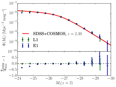
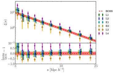
Throughout most of the following analysis, we focus our attention on several models in particular, parameterized in terms of $t_{0}$ and $\gamma$ as in Eqn. (3). The first four of these models have particularly good agreement with the BOSS measurements. The last two are included to demonstrate how the clustering signal changes as a function of $t_{0}$ for a fixed value of $\gamma$: models L1, L3, and L4 all have the same $\gamma$ value. We summarize these models in Table 3.

3. Clustering Measurements

3.1. Two-point Correlation Function

By construction, our method matches the input QLF at all redshifts, regardless of the individual properties of the underlying quasar population. However, we are not guaranteed to match the observed clustering of quasars. Changing the implicit mass-to-light ratio of Eqn. (10) through changing the quasar lifetimes will affect how halos are populated with quasars. In general, longer quasar lifetimes lead to quasars of the same luminosity being matched into hosts of larger masses. Since their hosts are more biased, this leads to quasars of the same luminosity showing a larger clustering signal. This is true at all luminosities. We want to match the clustering because it can affect the topology of reionization. There can also be spatial correlations present in the radiation field as a result of reionization, which are important for making measurements of the BAO from the Lyman-$\alpha$ forest (e.g., White et al. 2010; Slosar et al. 2013).

Here, we explore how to include clustering measurements from the two-point correlation function in our quasar catalog. Recent results from the BOSS survey for the clustering of quasars in the redshift range of interest are presented in White et al. (2012). The above work examines the clustering signal of quasars in both 2D-projected and 3D-redshift-space correlation functions at intermediate scales ($3\lesssim s\lesssim 25$ $h^{-1}$Mpc). The authors also introduce luminosity cuts to make the results more robust. For the purposes of this comparison, we consider their selection for which they imposed luminosity cuts on both the bright and faint ends, so that only objects with $-25\geq M_{i}\geq-27$ were considered across the entire redshift range (Sample 4 as defined by the authors). For a fair comparison, we impose similar cuts on our object selection. We also examine the redshift evolution of the results, and compare against the high-$z$/low-$z$ samples (Samples 5 and 6) as well. See Appendix B for further discussion of these different redshift samples.

Table 3A List of the Parameters of Some Quasar Models Considered.

Model Name	Light Curve	$\log_{10}(t_{0}/\mathrm{yr})$	$\gamma$
L1	Lightbulb	7.75	0
L2	Lightbulb	8.25	$-0.125$
E1	Exponential	7.25	0
E2	Exponential	7.75	$-0.15$
L3	Lightbulb	7	0
L4	Lightbulb	8.5	0

We explore the parameter space of available quasar models by examining the lightbulb and exponential light curves defined in Eqns. (1) and (2), as well as luminosity-dependent quasar lifetimes defined in Eqn. (3), parameterized by $t_{0}$ and $\gamma$. For each combination of parameters, we construct a quasar catalog in the manner described above. Then, we extract from this catalog all objects that satisfy the magnitude constraints at the central redshift of the survey $z=2.39$. This redshift represents the average redshift of quasars chosen in the BOSS sample; the actual quasar objects span in redshift from $2.2<z<2.8$. However, as noted in White et al. (2012), the redshift evolution of the signal is weak. Thus, extracting objects from our quasar catalogs at a single redshift rather than a range should have little effect on our overall conclusions. We measure the monopole of the two-point correlation function using the “natural estimator” $\xi$:

$$\xi(s)=\frac{\expectationvalue{DD(s)}}{\expectationvalue{RR(s)}}-1,$$ (16)

where $\expectationvalue{DD(s)}$ is the average number of quasar pairs from the quasar catalog separated by a real-space distance of $[s-\Delta s/2,s+\Delta s/2]$, and $\expectationvalue{RR(s)}$ is the number of pairs of points at the same separation drawn from a distribution with Poisson noise.

3.2. Calculating $\chi^{2}$ values

Figure 2.— The correlation matrix for the L1 model. Note how the matrix is dominated by the diagonal entries, which is to be expected for shot-noise dominated measurements. The small off-diagonal terms suggest that the covariance matrix has converged numerically, and should be stable when inverting. This type of structure is seen in all models considered.

In order to quantify the statistical uncertainty in our catalog, we ran a suite of 10 $N$-body simulations with different initial conditions. We then performed our abundance matching procedure on each of the different simulations, including several realizations for each volume. Since our abundance matching procedure stochastically determines which halos should be hosting active quasars at a given time step, we create several quasar catalogs for each individual halo catalog, using a different initial random seed (three realizations per volume for these results). Additionally, we have augmented the effective number of samples by including redshift space distortions along the different principal axes of the simulation. This strategy gives us a total of 90 samples for which to measure the clustering signal. The best estimate for the correlation function $\xi(s)$ for a given radial bin $s_{i}$ is given by averaging over all of the individual estimates $\xi_{k}$:

$$\bar{\xi}(s_{i})=\frac{1}{N}\sum_{k=1}^{N}\xi_{k}(s_{i})$$ (17)

We then estimate the covariance between the radial bins by computing the entries of the covariance matrix $C_{ij}$. We compute the entries of the covariance matrix as (Zehavi et al., 2005):

$$C_{ij}=\frac{1}{N}\sum_{k=1}^{N}\quantity(\xi_{k}(s_{i})-\bar{\xi}(s_{i}))\quantity(\xi_{k}(s_{j})-\bar{\xi}(s_{j})).$$ (18)

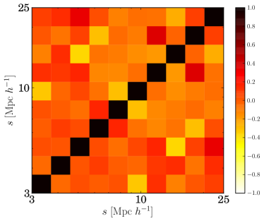
The correlation matrix entries for our model L1 is plotted in Figure 2. Notice that the diagonal entries dominate, which means that the bins are mostly independent of each other and dominated by shot-noise (Valageas et al., 2011; White et al., 2012). Implicitly, the samples have been treated as being independent, and this is almost surely not the case. Although the 10 volumes as a whole can be treated as being statistically independent, the different realizations based on the same halo catalog are likely correlated. Further, the projections of peculiar velocities along different axes for the same realization are also likely to produce correlated results. However, producing a sufficient number of independent realizations to decrease the noise in the covariance matrix is computationally infeasible. Further, the variance in the clustering signal among quasar catalog realizations for a given $(t_{0},\gamma)$ pair is comparable to small displacements in the $t_{0}$–$\gamma$ parameter space, so it is necessary to include this source of uncertainty. Since we are interested only in finding models that are consistent with the BOSS measurements which have their own set of observational uncertainties, we feel that this approach produces sufficiently accurate results.

Figure 3.— The quasar two-point correlation function from White et al. (2012), compared to several models whose parameters are described in Table 3. All measurements were made at the same values of $s$, but are offset from each other for visual clarity. The shaded error regions on the measurements from BOSS are the reported 1$\sigma$ error bars, and the error bars on the models are the square root of the diagonal elements of the covariance matrix. Note that for the same value of $\gamma$, increasing $t_{0}$ leads to a larger clustering signal (compare L3, L1, and L4 in order of increasing $t_{0}$). See the text for additional details.

Once the entries of the covariance matrix have been computed, the difference vector $\delta(s_{i})\equiv\xi_{\mathrm{model}}(s_{i})-\xi_{\mathrm{BOSS}}(s_{i})$ is calculated. The correlation function $\xi_{\mathrm{BOSS}}$ is fit to a power law: $\xi_{\mathrm{BOSS}}(s)=(s/s_{0})^{\beta}$, where the authors have fixed the value of $\beta=-2$. In order to investigate the impact this choice has on the conclusions, we performed fits on the correlation function measured from our quasar catalogs using two different parameterizations: one where the best-fit value of $s_{0}$ was found when fixing $\beta=-2$, and another where the value of $s_{0}$ and $\beta$ were both fit. In the length scales used for our analysis ($3\leq s\leq 25$), the deviation of $\beta$ from the fiducial value of $-2$ was small, typically less than 5%. Furthermore, the values for $s_{0}$ were also largely similar between a fixed slope or a varying one, with deviations typically less than 1%. Thus, the choice to set $\beta=-2$ does not strongly bias the results presented here, or the values reported in $\xi_{\mathrm{BOSS}}$.

When comparing one of the quasar models with the BOSS results, the $\chi^{2}$ value of the model is then given by:

$$\chi^{2}=\delta^{\mathrm{T}}C^{-1}\delta.$$ (19)

To define the model that fits the BOSS observations best, we want to minimize the $\chi^{2}$ value of the model. A two-dimensional space in $t_{0}$ and $\gamma$ is constructed for both of the light curves, and this space is explored using regular grid points. Following the analysis of White et al. (2012), a $\chi^{2}$ distribution with nine degrees of freedom is assumed. Using this distribution, the $\chi^{2}$ value for a particular model is converted to a confidence interval. An equivalent $n\sigma$ value is computed based on the confidence interval ($1\sigma$ if the enclosed probability is 0.683, $2\sigma$ if it is $0.955$, etc.). This statistic demonstrates how “consistent” a particular model is with the BOSS observations.

Figure 3 shows the clustering measurements for several of our well-fitting models compared to the BOSS measurements. The values of these models are given in Table 3. In general, as $t_{0}$ increases at a fixed value of $\gamma$, the clustering signal increases as well. Compare specifically the L3, L1, and L4 models, which have the same value of $\gamma$ but have respectively increasing values of $t_{0}$. Mathematically, this behavior can be seen from the form of Eqn. (10): for the same luminosity and mass functions but a larger value of $f_{\mathrm{on}}\propto t_{q}$, quasars of the same luminosity will shift to more massive host halos. Since the clustering signal increases with the mass, it follows that increasing $t_{0}$ will increase the clustering signal. For similar reasons, increasing values of $\gamma$ for constant values of $t_{0}$ are also associated with a stronger clustering signal, since this also effectively increases the quasar lifetime $t_{q}$.

Figure 4.— A comparison of the parameter space exploration in terms of the parameters $t_{0}$ and $\gamma$ from Eqn. (3). Both the parameter space for the lightbulb model (Eqn. (1)) and exponential model (Eqn. (2)) are shown. The dashed lines represent the best linear fits to the data for a particular light curve. The class of models that are consistent with the BOSS measurements at $1\sigma$ and $2\sigma$ correspond to the darkly and lightly shaded regions. In general, we find that for the exponential model, shorter lifetimes are preferred (smaller values of $t_{0}$ for the same $\gamma$). Since we abundance match against the quasar’s peak luminosity, and the quasar spends comparatively little time at or near the peak luminosity, we effectively increase the clustering signal for lower luminosity quasars.

3.3. Characteristic luminosity and lifetime

Table 4A List of the Best-fit Parameters for Our Quasar Model as a Function of Redshift.

Redshift Selection	$z_{\mathrm{eff}}$	Light Curve	$L_{\mathrm{eff}}^{*}$	$t_{\mathrm{eff}}^{*}$
High-$z$	2.51	Lightbulb	$12.92$	7.62
		Exp	$12.40$	7.14
Fiducial	2.39	Lightbulb	$13.29$	7.77
		Exp	$13.05$	7.18
Low-$z$	2.28	Lightbulb	$13.17$	7.84
		Exp	$13.15$	7.29

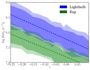
Figure 4 shows the $\chi^{2}$ values in the two-dimensional parameter space $t_{0}$ and $\gamma$, as defined by Eqn. (3), for the different light curves. The region of good agreement between the BOSS measurements and our models takes on a linear relationship between $\log_{10}(t_{0})$ and $\gamma$. Such a relationship can be parameterized as:

$$\log_{10}(t_{0}/\mathrm{yr})=\log_{10}(t_{\mathrm{eff}}/\mathrm{yr})+L_{0}\gamma.$$ (20)

The parameters $t_{\mathrm{eff}}$ and $L_{0}$ can be thought of as a characteristic timescale and a characteristic luminosity, respectively. From the functional form of our power-law for quasar lifetime in Eqn. (3), $L_{0}$ can be interpreted as changing the normalization luminosity. This is the luminosity at which all models have the same lifetime, regardless of the value of $\gamma$. In other words, the characteristic luminosity of the power law becomes:

$$\log_{10}(L_{\mathrm{eff}}/L_{\odot})=10-L_{0},$$ (21)

where $L_{0}$ is defined in Eqn. (20). The parameter $t_{\mathrm{eff}}$ is the characteristic time because all models have this same lifetime at the luminosity $L_{\mathrm{eff}}$.

For the lightbulb model, the best-fit values are $\log_{10}(t_{\mathrm{eff}}/\mathrm{yr})=7.76$ and $\log_{10}(L_{\mathrm{eff}}/L_{\odot})=13.29$. (See Table 4 for evolution of these parameters with redshift.) The characteristic luminosity inferred from this value is $L_{\mathrm{eff}}=10^{13.29}\ L_{\odot}$, which has a corresponding magnitude of $M_{i}=-27.2$. This value is not surprising, given that quasars were selected for the clustering measurements near this magnitude range. More interesting is the value of $\log_{10}(t_{\mathrm{eff}}/\mathrm{yr})=7.77$, which gives a characteristic lifetime of $10^{7.77}=59$ Myr. This is a quasar lifetime that is slightly longer than those typically quoted in the literature (Yu & Tremaine, 2002; Porciani et al., 2004; Yu & Lu, 2004; Conroy & White, 2013), which are closer to the Salpeter $e$-folding time scale or shorter ($\sim$45 Myr for a quasar accreting at Eddington luminosity and a mass conversion efficiency of $\epsilon=0.1$). Although $t_{\mathrm{eff}}$ is slightly higher than these values, it is within a factor of 2.

Figure 5.— The range of quasar lifetimes for models with the best-fit values of $t_{0}$ as a function of $\gamma$, based on the linear relationship extracted in Eqn. (20). The solid regions show the span in quasar lifetimes, while the dashed line shows the median value within a given model. Note that the median value is fairly constant across all quasar lifetimes. Thus we are able to characterize a quasar model reasonably well using the characteristic lifetime. The comparative large spread in quasar lifetime in the exponential case is due to our method of selecting $t_{q}$, rather than reflecting a truly large spread in the data. See the text for additional details.

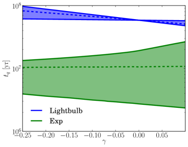
In the exponential model, the best-fit values for $t_{\mathrm{eff}}$ and $L_{\mathrm{eff}}$ defined in Eqn (20) are $\log_{10}(t_{\mathrm{eff}}/\mathrm{yr})=7.18$ and $\log_{10}(L_{\mathrm{eff}}/L_{\odot})=13.05$. This luminosity implies a slightly dimmer characteristic luminosity ($M_{i}=-26.6$). As discussed in Sec. 2.4, there is not a single $\tau$ for all quasars for a given value of $t_{\mathrm{eff}}$: $L\approx L^{*}$ quasars have $\tau\approx t_{\mathrm{eff}}$, with brighter quasars having $\tau>t_{\mathrm{eff}}$. However, the difference between $\tau$ and $t_{\mathrm{eff}}$ does not differ by more than a factor of 2 in either direction, and so to a good approximation $\tau\sim t_{\mathrm{eff}}$, especially for the luminosity range used to match the clustering measurements. Compared to the lightbulb case, the quasars with an exponential light curve have a shorter characteristic lifetime of 15.1 Myr. The characteristic lifetime is smaller for the exponential than in the lightbulb case because quasars do not shut off entirely after a single lifetime, so the time that a quasar is “bright enough” to be included within the luminosity cuts is longer than its lifetime $t_{\mathrm{eff}}$. This lifetime is about a third of the Salpeter $e$-folding time scale, which implies that if quasar light curves are roughly exponential, the combination of the measured QLF and the clustering measurements favors quasars that either radiate at luminosities dimmer than their Eddington ratio ($L/L_{\mathrm{edd}}<1$), have a mass-conversion efficiency that is less that the fiducial value ($\epsilon<0.1$), or both. Unfortunately, since our model does not track the underlying physics present, we are not able to distinguish between these two cases.

The reason for the different best-fit values between the two models can be understood as follows. By construction, we have fixed the lifetime of the exponential quasars such that their peak luminosity-to-mass ratio is the same as in the case of the lightbulb for a given choice of $t_{0}$ and $\gamma$. (See Sec. 2.4 for more details.) However, the mass-to-light ratios for the two light curves are significantly different. This is due to the fact that the observed luminosity for an exponential quasar can be much smaller than its peak luminosity. A particular luminosity range is selected for the clustering measurements, but the clustering of these quasars is tied to their peak luminosity rather than the observed one. Thus, quasars will tend to have higher clustering at a given luminosity in the exponential case compared to the lightbulb, since they spend comparatively little time at or near their peak luminosity. This luminosity selection includes quasars with a higher peak luminosity than the chosen range (and thus a higher clustering signal), so we must also include quasars that have lower mass hosts to match the average clustering signal. This means that there is a larger spread in host mass compared to the lightbulb case. This behavior explains why the characteristic luminosity is slightly smaller for the exponential model compared to the lightbulb: there is an increased number of low-luminosity quasars occupying high-mass hosts.

Figure 5 shows the range of quasar lifetimes as a function of model parameter $\gamma$. The quasar lifetime is broadly similar across different model choices. The exponential model has a lower overall value due to the effect discussed above, i.e., that quasars from a higher peak luminosity will be included in the sample, bringing along a higher clustering signal. Since this is true for nearly all the quasars in the sample, there is an overall decrease in the selected lifetime of quasars. The large difference in the span of quasar lifetimes is due to the way that we have defined the quasar lifetime in the exponential model. As discussed in Sec. 2.4, the exponential lifetime $\tau$ is selected such that the same relationship between host mass and quasar peak luminosity exists in the exponential case as in the lightbulb case. Even in a model where for the lightbulb $t_{q}$ is independent of $L$ (i.e., when $\gamma=0$), the exponential model parameter $\tau$ does have luminosity dependence. In general, quasars with luminosities above $L_{*}$ will have a lifetime longer than an equivalent luminosity in the lightbulb case for the same choice of $t_{0}$ and $\gamma$ in Eqn. (3), and those with low luminosities will have a shorter lifetime. This choice for our model leads to the spread in lifetimes of a factor of $\sim$5, as seen in the case of $\gamma=0$. For models in which $\gamma>0$, there is a widening in the range of values. This is due to the fact that brighter quasars live longer than dimmer ones. Since our choice of quasar lifetime already enforces this difference, these models see an increased effect. Conversely, for $\gamma<0$, there are competing effects between brighter quasars being less long-lived due to the choice of $\gamma$, but still simultaneously living longer than their lightbulb counterparts due to the choice of $t_{q}$. The latter effect wins out, and these quasars end up having a significantly larger spread than in the lightbulb case. Note that the contours in this figure are smooth compared to Fig. 4 because these are results lying along the best-fit line, and the figure shows the range in values rather than a single number (i.e., the $\chi^{2}$ value) that fluctuates as a function of position in $t_{0}$ and $\gamma$.

4. Discussion

4.1. Mass-to-light Ratio

The combination of the QLF and clustering measurements produces an important set of constraints on the space of potential quasar models. Here we investigate the implications of these models. One important implication is the mass of a typical halo for a given quasar luminosity. It is trivial to predict this for the case of a lightbulb model, but less straightforward for the case of the exponential model. Here the peak luminosity $L_{\mathrm{peak}}$ is used to define the mass-to-light ratio, since this is the quantity used in our abundance matching approach. This ratio defines a typical mass for quasars, which can be compared with results of previous analysis (e.g., Martini & Weinberg 2001; Shen et al. 2007; White et al. 2012).

Figure 6.— A comparison of the mass-to-light ratio between the different quasar models. We have computed this ratio for each model in our parameter space, and weighted their contribution by their corresponding $\chi^{2}$ value. The lines show the median value by weight and the shaded regions show $\pm 1\sigma$ and $2\sigma$. Note that for a given luminosity, a quasar in the exponential model is found in a halo with a smaller mass. This is due to the fact that quasars with a peak luminosity significantly greater than the observed one are included in the luminosity range selected for the clustering measurements. These hosts have a higher clustering signal than quasars with a peak luminosity in the luminosity selection. This means we must also select lower-mass objects as well. See the text for additional details.

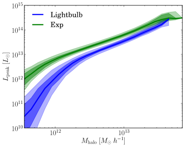
Figure 6 shows the luminosity of quasars as a function of the mass of the host halo for the lightbulb and exponential models for all combinations of $t_{0}$ and $\gamma$. This plot shows the mass-to-light ratio of the entire catalog. The weight assigned to the luminosity as a function of mass $L_{\mathrm{peak}}(M)$ for a particular model $i$ is given by a $\chi^{2}$ likelihood. We also find the $\pm$ 1 and 2 $\sigma$ values that enclose 68% and 95% of the likelihood.

Figure 7 shows the mass range as a function of the model parameter $\gamma$. Note that the range is essentially constant with respect to $\gamma$. By averaging the median mass across all values of $\gamma$, a characteristic mass for the two models can be defined. This characteristic mass is $2.5\times 10^{12}$ $h^{-1}M_{\odot}$ for the lightbulb model, and $2.3\times 10^{12}$ $h^{-1}M_{\odot}$ for the exponential model. These values are broadly consistent with previous studies of quasar clustering measurements (e.g., Porciani et al. 2004; Croom et al. 2005; Lidz et al. 2006; Porciani & Norberg 2006; White et al. 2012). Since in all models the same clustering signal of the quasars is being selected, there is an implicit requirement for the hosts to lie within a certain mass range. Additionally, the mass range in the exponential case is significantly larger than that of the lightbulb model. This is again related to the fact that due to the light curve, quasars with a higher clustering signal are included within the luminosity sample, and so there must also be lower-mass hosts included as well to balance the average clustering strength. There is a significantly larger spread above the median mass than below. The reason for this asymmetry is due to the difference in number density: since the high-mass objects are rarer, a comparatively smaller range in low-mass halos is necessary to make the clustering signal equivalent to the lightbulb case. See Sec. 3.3 for further discussion.

Figure 7.— The selected mass range for our different models. For the lightbulb case, there is a relatively narrow range in mass. Since the clustering of quasars is fixed as a function of luminosity, there is a very tight relationship between observed luminosity and underlying host mass. In the exponential case, the range is much more extended. Since the mass-to-light ratio is fixed to be the same for the peak luminosity, the evolution within the model means that there will be quasars with higher peak luminosity (and higher-mass hosts) selected by the evolution.

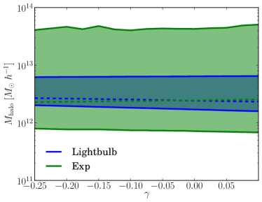
In the case of the lightbulb model, the halo mass that corresponds to the selected luminosity range of quasars is relatively tightly constrained. For the models that agree with the BOSS measurements at $1\sigma$, the average halo mass ranges from 1.35 $\times$ 10¹² to 4.93 $\times$ 10¹² $h^{-1}M_{\odot}$ for hosts of quasars within the magnitude cutoff. For the exponential model, there is a much larger range in halo mass: for the collection of models that agree at $1\sigma$, the mass ranges between 6.69 $\times$ 10¹² and 5.85 $\times$ 10¹³ $h^{-1}M_{\odot}$, almost an entire order of magnitude (compared to about half an order of magnitude for the lightbulb model). Also note that the mass range is much larger than in the lightbulb case. This fact can be explained by noting that there is evolution in the mass-to-luminosity ratio during the lifetime of the quasar. Further, the $e$-folding time for these models is comparatively long, with typical values being $\tau\approx 40$ Myr. This means that there are high-mass hosts included in the sample of quasars chosen for the clustering measurements whose quasars are not at their peak luminosity. Since these hosts have a bias larger than the value preferred by the BOSS measurements, this sample must necessarily include hosts which have a smaller clustering signal, so that on average, the total bias agrees with BOSS.

There is a systematic shift upward in the mass of the exponential case compared to the lightbulb. This shift is related to the difference in parameter space discussed in Sec. 3.1. Due to their exponential change in luminosity, the quasars are not typically found near their peak luminosities. Thus, even though by construction the peak quasar luminosity as a function of halo mass is the same for the two models, the effective luminosity for a given mass is reduced in the exponential case due to the light curve evolution. In other words, quasars of the same luminosity in the two different models are found in more massive hosts in the exponential case. This leads to a systematic shift in the preferred mass range for clustering measurements. To sum up: the increased spread in halo host mass for the exponential model compared to the lightbulb is due to inclusion of highly biased hosts in the measurement being balanced out by lower-mass ones, and the systematic shift toward higher mass is due to the effective increase in the mass-to-luminosity ratio related to evolution of quasar luminosity.

4.2. Mass function and duty cycle of halo hosts

Figure 8.— The halo mass function for halos hosting quasars versus the total halo population for certain models as defined in Table 3. In the case of the lightbulb model, there is a roughly constant value of $\sim$1% of halos hosting quasars as a function of halo mass. For the exponential, there is a constant active fraction at the high-mass end, but then the fraction falls off below the median halo mass. This is again related to the fact that there are more halos included at low mass in order to reproduce the average clustering signal.

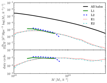
To observe the effect that different points in parameter space have on the halo host properties, the mass function of halos hosting an active quasar has been calculated for the fiducial redshift selection. (For the high- and low-redshift selections, see Appendix B.) Figure 8 shows the total halo mass function as well as the mass function of halos hosting quasars within the luminosity range $-25\geq M_{i}\geq-27$. From this analysis, the duty cycle of halo hosts can be extracted, i.e., the fraction of active halos divided by the total number of halos. As discussed in Sec. 2.2, in the lightbulb model the duty cycle can be directly related to the quasar lifetime at that luminosity. However, here the duty cycle is defined simply as the active fraction of halos.

Figure 8 compares the case of the lightbulb and the exponential light curves. When the halo mass function of active halos is examined in the two different cases, it can be seen that the mass range of hosts spanned by an individual model is quite different. In the lightbulb case, there is a very small range in host mass compared to the exponential case. This difference can be explained in terms of which hosts are included in the clustering measurements. In the lightbulb case, since the luminosity is constant as a function of quasar lifetime, the only evolution in the relationship between mass and luminosity comes from mass accretion, which makes up a small fraction of total halo mass over the time scales for which quasars are active. As such, with an essentially static relationship, there is a very strong correlation of mass to light. For a specific model, there is only about a factor of 2 in halo mass included for the quasars in the selected magnitude range. When looking at the duty cycle of quasar hosts, one can see that the fraction is typically 0.5-1%, with little evolution with mass within a model.

Conversely, in the exponential model, there is evolution for individual halos in the mass-to-light relationship. Most importantly, this implies that massive halos will be included when selecting quasars at a specific luminosity. Since they are more highly clustered (and more biased), smaller, less biased halos must also be included in order to create an average bias consistent with the BOSS measurements. This has the effect of extending the mass range of halos included in the mass function. Note that within a single model, there is a much larger span in halo mass: in some cases, the span is more than an order of magnitude in halo mass. Additionally, the duty cycle is comparable in magnitude to the lightbulb case, though slightly smaller: the ratio of active halos to total halos ranges from 0.05-1%. There also seems to be a trend in the evolution of the duty cycle: there is a central “typical mass” for a given model, and the duty cycle decreases in both directions. A similar trend was found by White et al. (2012).

Note that one result of this measurement is the fact that the mass range of host halos is significantly more extended in the exponential case than the lightbulb case. Thus, one way to break the degeneracy between the lightbulb and exponential models would be to measure the mass range of underlying host halos, perhaps through using gravitational lensing to independently find the mass of the dark matter halo (Courbin et al., 2012). If the range of masses for quasar hosts is extended, then there would be observational evidence favoring an exponential model (or a model with evolution in the quasar light curve) as opposed to the lightbulb model.

5. Predictions for Helium Reionization

QLF:

$L_{912}$ normalization:

SED spectral index:

Clumping factor:

Figure 9.— The volume-filling fraction $Q_{i}$ of doubly ionized helium defined in Eqn. (22). In each plot, we show the fiducial values we have for $Q_{i}$ as a function of redshift, which has the parameters $\alpha=1.7$, $\bar{C}=3$, and normalizing the luminosity at 912 Å following Lusso et al. (2015). This leads to a redshift of reionization of $z\sim 2.5$, comparable to the redshift of $z\sim 2.7$ suggested by observation of the helium Lyman-$\alpha$ forest. We show the change in $Q_{i}$ as a function of varying these parameters. Top left: we compare the difference between using the composite QLF of SDSS+COSMOS (see Sec. 2.5 for more details) and the one in Hopkins et al. (2007). The shaded region reflects differences in ionization level due to jointly varying the parameters over the ranges specified in Table 2. Top right: we change the UV SED of the quasar, which affects the normalization at 912 Å. In addition to the SEDs from Lusso et al. (2015) and HRH07, we show the radio-quiet template from Shang et al. (2011). Bottom left: we allow the EUV SED spectral index for $\lambda<912$ Å to vary from $1.4\leq\alpha\leq 2.0$. Bottom right: we vary the clumping factor of the IGM, from $1\leq\bar{C}\leq 5$. See the text for additional details.

One very important prediction that we can make from our quasar catalog is the redshift of helium reionization. In order to understand in detail the implications for helium reionization, we need to run full hydrodynamic plus radiative transfer numerical simulations. However, we can perform a semi-analytic calculation in order to find a rough estimate of the redshift of reionization by computing the fraction $Q_{i}$ of the universe’s volume that has been reionized (also called the volume-filling fraction), where $Q_{i}=1$ represents a totally reionized universe (e.g., Madau et al. 1999; Furlanetto & Oh 2008):

$$\derivative{Q_{i}}{t}=\int\differential{L}\frac{\dot{N}_{\gamma}}{\bar{n}_{\mathrm{He}}}\derivative{\phi}{L}-\bar{C}\alpha_{A}\bar{n}_{e}Q_{i},$$ (22)

where $\bar{n}_{\mathrm{He}}$ is the number density of neutral helium, $\bar{n}_{e}$ is the number density of electrons, $\dot{N}_{\gamma}$ is the production rate of ionizing photons for an individual quasar, $\alpha_{A}(T)$ is the recombination coefficient, and $\bar{C}\equiv\expectationvalue{n_{e}^{2}}/\expectationvalue{n_{e}}^{2}$ is the clumping factor of the ionized IGM. The minimum luminosity of the integral decreases as redshift decreases, in keeping with modeling and observations (Richardson et al., 2012; Shen & Kelly, 2012; Cen & Safarzadeh, 2015; Sijacki et al., 2015). The clumping factor measures the effective distribution of gas inside the scale of volume being averaged (or resolution in the case of simulations). Note that these calculations assume a primordial helium mass fraction of $Y_{\mathrm{He}}=0.24$. Following the arguments in the appendix of Kaurov & Gnedin (2014), we choose the case A recombination coefficient, which assumes that photons emitted from recombination are not reabsorbed by a neutral atom, increasing the recombination rate. It is assumed that initially, all of the hydrogen in the IGM has been ionized, and all of the helium is singly ionized. To compute the photoionization rate of an individual quasar $\dot{N}_{\gamma}$, the SED of Lusso et al. (2015) is used to convert the specific luminosity at 2500 Å to that at 912 Å. It is then assumed that quasars have an SED that follows a power law $L_{\nu}(\nu)\propto\nu^{-\alpha}$ for values of $\lambda<912$ Å. The fiducial value chosen is $\alpha=1.7$, also based on observations of the rest-frame UV spectra of quasars from Lusso et al. (2015). This calculation includes all photons with frequencies in the range 54.4 eV $\leq$ $h\nu$ $\leq$ 1 keV. Photons above this energy have a mean free path of helium ionization comparable to the Hubble distance.

Although the two different quasar light curves explored above have different individual properties, both are constrained by the global properties fixed by the QLF. We find that if instead of the statistical calculation outlined above, we use the number of ionizing photons computed directly from the quasar catalogs, the result differs only by a few percent. Therefore, it is much more straightforward to use Eqn. (22). This approach also permits the use of other QLFs in the calculation, so it is possible to explore what effect this has on the results.

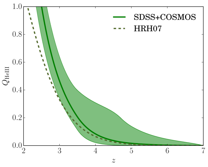
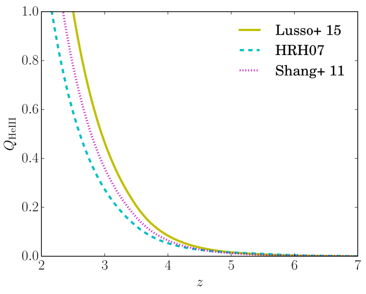
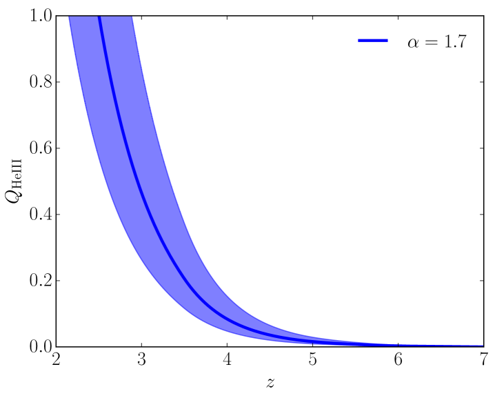
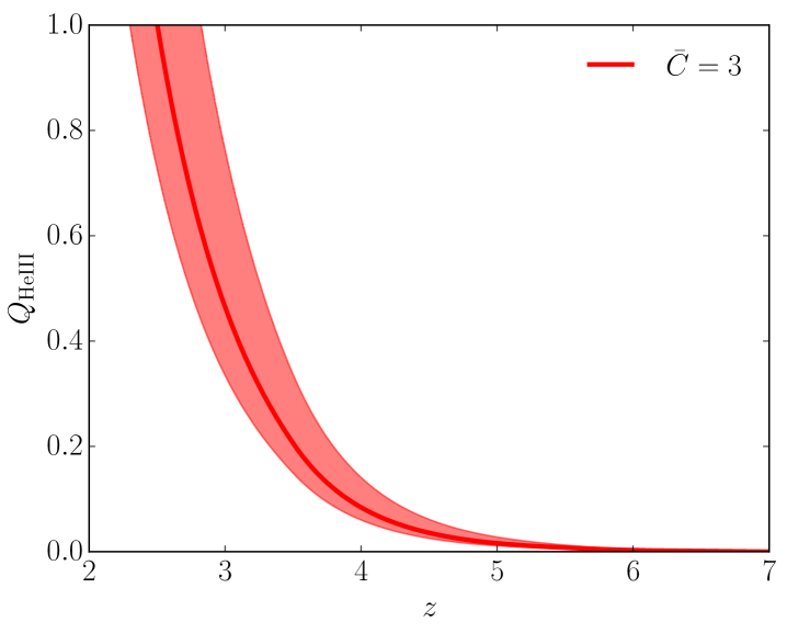
Figure 9 shows the ionization fraction as a function of redshift computed from Eqn. (22). In the first panel, there is a comparison of the choice of QLF used in the calculation. Included are the QLF used in the main body of this work, the composite QLF composed of the ones from R13, M12, and M13 (the SDSS+COSMOS) as explained in Sec. 2.5, and the QLF from Hopkins et al. (2007) (hereafter referred to as HRH07). All other calculations presented use the composite QLF, but then change various other parameters. Note that for the prediction of reionization time using HRH07, both the QLF and the SED are different from the fiducial comparison case. In the figure, the shaded region shows the range of predicted values for the volume-filling fraction $Q_{i}$ at a given redshift $z$ by jointly varying the parameters of the QLF over the range specified by Table 2. Interestingly, the late-time ionization level is less sensitive to the variation in parameters at early redshift, due to the interplay between the source and recombination terms present in Eqn. (22). At redshifts $z\leq 3.5$, the source term becomes the same for all histories, since the QLF transitions to that of Ross et al. Further, the recombination rate is proportional to the ionized fraction, so histories that had higher ionization levels at $z\geq 3.5$ will have higher levels of recombination. Since the recombination time is much shorter than the total timescale of the reionization calculation, all histories converge on a similar redshift of total reionization ($Q_{i}=1$). Nevertheless, the variation in ionization fraction at early times can have important implications on the topology of ionized regions and the thermal history of the IGM, so such differences may in principle be detectable.

In the second panel of the plot, the specific luminosity of individual objects at 912 Å $L_{912}$ is varied. One way to achieve this variation is the change the UV SED template used for quasars. Once the specific luminosity $L_{2500}$ is calculated from the observed magnitude according to Eqn. (7), the quasar SED can be used to find $L_{912}$. In the fiducial approach, we use the SED template from Lusso et al. (2015), which assumes a UV spectral index of $\alpha=0.61$ for $2500\ \mathrm{\AA}\geq\lambda\geq 912\ \mathrm{\AA}$. An alternative choice for an SED is one from Shang et al. (2011), which provides a composite quasar SED template by combining observations in different frequency ranges to create a single spectrum. Shang et al. (2011) divide the sample into radio-loud and radio-quiet quasars. However, radio-quiet quasars compose $\sim 90\%$ of high-redshift quasars found in the SDSS (Shen et al., 2009). Thus, we only include the results of the calculation using the radio-quiet template. This template provides the relative specific luminosity at each frequency, and so can be used to convert $L_{2500}$ to $L_{912}$. The effective spectral index for this wavelength range for the radio-quiet quasar template is $\alpha=0.867$. In addition, we show the impact of using the SED from HRH07 (with the QLF from Sec. 2.5). Note that the SED from HRH07 is outdated, and used only as a point of comparison. More recent studies (e.g., Stevans et al. 2014; Lusso et al. 2015) are largely inconsistent with the SED of HRH07, and so it is presented here merely to emphasize the importance that using the proper SED has on helium reionization. Given this same specific luminosity $L_{2500}$, the predicted value of $L_{912}$ from the SED of Lusso et al. (2015) is higher than that of HRH07 by about a factor of 1.7, leading to the earlier reionization time. The second panel of the plot includes these to demonstrate the difference from using different quasar templates.

In the third panel of the plot, the spectral indices are varied, ranging from $1.4\leq\alpha\leq 2.0$. Recent measurements from Lusso et al. (2015) suggest that at high redshift and bright magnitudes, the spectral index has a value of $\alpha=1.7\pm 0.6$. This is slightly softer than the average value of $\alpha=1.6$ from Telfer et al. (2002). In order to explore some of the implications of changing the spectral index, we vary its value as indicated.

The final panel explores a range of clumping values, from $1\leq\bar{C}\leq 5$. The precise value for the clumping factor for helium reionization is very uncertain, as most studies on the clumping factor are related to hydrogen reionization (see, e.g., Raičević & Theuns 2011; Kaurov & Gnedin 2014). In Furlanetto & Oh (2008), the authors explored clumping factors of $0\leq\bar{C}\leq 3$. More recent results from numerical simulations were calculated by Jeeson-Daniel et al. (2014), who found that the clumping factor of helium ranges from $3\leq\bar{C}\leq 8$ for the redshift range of interest, depending on the ionization level of the helium gas.

In Figure 9, each panel shows the fiducial evolution of $Q_{i}$, which is characterized by the values of $\alpha=1.7$, $\bar{C}=3$, the SED of Lusso et al. (2015), and the composite SDSS+COSMOS QLF. In this situation, the redshift of reionization (i.e., when $Q_{i}=1$) is $z\sim 2.5$. This value is comparable to, though slightly later than, the redshift suggested by recent observations of $z\sim 2.7$ (Dixon & Furlanetto, 2009; Worseck et al., 2011). However, a smaller volume-averaged clumping factor $\bar{C}$ or a larger amplitude in either the measured QLF or the specific luminosity $L_{912}$ could give an earlier redshift of reionization. Specifically, assuming the fiducial model, changing the clumping factor to $\bar{C}=1.7$ would give $z\sim 2.7$ as the redshift of reionization. It should be noted that this calculation is not wholly accurate for reionization, since it assumes a single clumping factor for the entire IGM, which is almost certainly not accurate for helium reionization, due to its very inhomogeneous nature. Furthermore, this calculation does not include secondary ionizations from energetic electrons (e.g., Shull 1979; Furlanetto & Stoever 2010), though these interactions are likely unimportant for helium reionization (McQuinn et al., 2009).

When comparing to the results of Furlanetto & Oh (2008), we notice that the authors’ value for the redshift of reionization is significantly earlier than the one that we have found. This is largely due to a different QLF used, as well as a different method for calculating a quasar’s EUV SED. The referenced paper uses the QLF from HRH07, and assumes an SED that gives more EUV radiation. This luminosity function has a significantly larger amplitude compared to the results from R13, up to an order of magnitude larger for low-luminosity quasars at high redshift. (See Fig. 16 of Ross et al. 2013.) Thus, accurate measurements and a proper understanding of the systematics of the high-redshift QLF, as well as the accompanying quasar SED, are essential for a proper treatment of helium reionization.

6. Conclusion

We have provided a technique for populating dark matter halos with quasars that matches a QLF by construction for various light curve models of quasars. By using the triggering rate of Hopkins et al. (2006) with the technique of abundance matching, we are able to match the observed QLF of SDSS Data Release 9 (DR9) (R13), COSMOS (M12), and high-redshift SDSS data (M13). After applying this method to dark matter halo catalogs generated from $N$-body simulations, we have constrained a class of quasar models that reproduce the clustering amplitude measured from the two-point auto-correlation function of the BOSS survey (White et al., 2012) at a redshift of $z=2.39$. The characteristic mass of the quasar hosts is $2.5\times 10^{12}$ $h^{-1}M_{\odot}$ for the lightbulb model and $2.3\times 10^{12}\ h^{-1}M_{\odot}$ for the exponential model. The effective lifetime as defined in Eqn. (20) of quasars is $t_{\mathrm{eff}}=59$ Myr for the lightbulb model of quasars and $t_{\mathrm{eff}}=15$ Myr for the symmetric exponential model.

One of the limitations of this approach is that we have constrained the class of quasar models using a comparatively narrow span in quasar luminosity. By matching the bias of quasars with a different magnitude range, we would have a different effective luminosity range for the bias calculation. This would lead to a different slope in the parameter $L_{\mathrm{eff}}$, which would allow us to break the degeneracy observed in Fig. 4. Having the ability to break the sample down into different luminosity intervals would allow us to make tighter constraints on the class of allowed models.

In future work, we plan to use the quasar models explored here as sources of ionizing photons for studying helium reionization using simulations containing hydrodynamics and radiative transfer. These types of simulations will allow us to accurately capture important physical characteristics related to the IGM. Specifically, we are interested in capturing the thermal history of the IGM as it relates to observations. In upcoming simulations, we plan to compute the IGM equation of state and produce synthetic Lyman-$\alpha$ forest fluxes. This will allow us to tap into the wealth of observations available for the Lyman-$\alpha$ forest, such as those currently available from BOSS (e.g., Lee et al. 2013), and from upcoming future surveys such as DESI.

Appendix A Fitting the parameters of the QLF

In order to construct a QLF informed by the observations at all redshifts relevant to helium reionization, we have combined the measurements of R13, M12, and M13. We will now briefly summarize the relevant findings of each paper. In all three results, the QLF is parameterized as a double-power law, according to Eqn. (11). R13 uses quasars identified from SDSS-III DR9, and provides a LEDE model in which the base-10 logarithm of the QLF normalization, $\log_{10}\phi^{*}$, and the break magnitude $M^{*}$, evolve linearly with redshift, as parameterized in Equations (12) and (13). The parameters $\alpha$ and $\beta$ are fixed as a function of redshift. Nominally, the LEDE fit is valid over the redshift range $2.2\leq z\leq 3.5$. M12 uses data from the COSMOS survey, and measures the four QLF parameters at $z\sim 3.2$ and $z\sim 4$. M13 uses quasars identified in SDSS data in Stripe 82 (S82), and reports the four QLF parameters at $z\sim 5$. For all three results, the parameters themselves and their associated 1$\sigma$ uncertainties are reported. In the M13 results, the authors actually provide three different fits to the observed results. In their fiducial result, they fix the value of $\beta$, and fit for the three parameters $\log_{10}\phi^{*}$, $M^{*}$, and $\alpha$. In a second set of parameters, the authors fix the value of $\alpha$ and find the best-fit values for the other three quantities. Finally, the authors fix $M^{*}$, $\alpha$, and $\beta$, and only fit for $\log_{10}\phi^{*}$. The best-fit values for the parameters change significantly in some cases between the different fits. More importantly, none of these fits seems to be ruled out conclusively by the data presented in M13, and so we incorporate all of the fits in our results.

Figure 10.— A plot of the evolution of the QLF parameters as a function of redshift: the base-ten logarithm of $\phi^{*}$ (top left), the break magnitude $M^{*}$ (top right), the faint-end slope $\alpha$ (bottom left), and the steep-end slope $\beta$ (bottom right). Best-fit values and associated 1$\sigma$ errors from R13, M12, and M13 are represented as the solid lines with shaded error regions, dark-gray triangles, and light-gray stars, respectively. For the M13 data, all three sets of parameters provided by the authors are plotted at $z\sim 5$, slightly offset for visual clarity. The dashed lines for $z>3.5$ show the fiducial evolution of the QLF, and the dotted lines show the bracketing ranges of values explored. See the text in this appendix for further details.

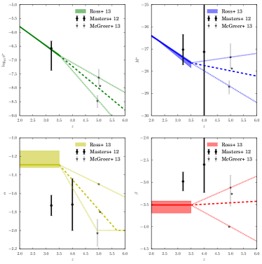
As explained in Sec. 2.5, our goal is to combine the observational data from different epochs. For redshifts $z\leq 3.5$, the parameters from R13 are used. At higher redshift, the parameters are assumed to vary linearly in redshift. The equations for the parameters are given in Eqns. (15a-15d). The constant values are taken to be those of R13 at $z=3.5$, and the slope of the redshift evolution is allowed to take on a range of values. We will now discuss each of the four parameters in turn.

For the parameter $\log_{10}\phi^{*}$, the fiducial value for the slope $c_{1}$ is chosen to reproduce the average of the three reported values of M13 at $z\sim 5$. As discussed in M13, the fits from R13 extrapolated to $z\sim 5$ do not reproduce the overall normalization well, and predict too high a number density. Thus, a steeper value than that of R13 is necessary. The range of values for $c_{1}$ are chosen to bracket the range of best-fit values reported by M13.

For the parameter $M^{*}$, the fiducial value of the slope $c_{2}$ is chosen to reproduce the average of the three reported values of M13 at $z\sim 5$. The slope is allowed to take on a range of values that bracket the three reported values of M13. Also note that we have converted between magnitude systems using $M_{i}(z=2)=M_{1450}-1.486$, which assumes a spectral index $\alpha=0.5$. If instead the value of $\alpha=0.61$ is used, as suggested by Lusso et al. (2015) and used in the calculations of Sec. 5, then conversion is $M_{i}(z=2)=M_{1450}-1.681$. Further, if the SED from Shang et al. (2011) is used, the conversion is $M_{i}(z=2)=M_{1450}-2.139$. The reason for the differences is that the $K$-corrections depend on the spectral index of the SED (see Eqn. 3 of Richards et al. 2006). By extension, the QLF can be affected when combining different data sets. However, to be consistent with previous works that have combined disparate data sets in this manner (e.g., R13 and M13), we use the conversion given by assuming $\alpha=0.5$.

For the parameter $\alpha$, the fiducial value of the slope $c_{3}$ is chosen to reproduce the average of the three reported values of M13 at $z\sim 5$. As with the other parameters discussed, a range of values is also explored which brackets all of the reported values of M13. Further, the value of $\alpha$ is bounded to lie where $\alpha>-2$. For $\alpha\leq-2$, the QLF does not converge for low-luminosity objects, and a cutoff luminosity must be specified below which quasars do not contribute significantly to helium reionization. To avoid defining such a cutoff luminosity, the value of $\alpha$ is bounded. As a practical matter, the ultimate goal of this project is to study helium reionization using full numerical simulations, where the minimum resolved halo mass will set the lower-limit of quasar luminosities.

Finally, for the parameter $\beta$, the fiducial value for the slope $c_{4}$ is chosen to reproduce the average of the values from M13 at $z\sim 5$. The range of slopes is chosen to bracket the values reported by M13. For the fiducial choice of slope, the value of $\beta$ does not vary significantly with redshift. This range of values incorporates much of the parameter space constrained by M13, without the values of $\beta$ becoming arbitrarily steep. However, the choice of $\beta$ ultimately does not significantly affect the ionization level predicted by Eqn. (22).

As a final note, the values of $\alpha$ and $\beta$ at $z\sim 3.2$ from M12 are nominally inconsistent with the combined results from R13. However, when looking at the results for individual redshift bins at $z\sim 3.2$ (e.g., Fig. 15 from R13), the uncertainties for the R13 values are significantly larger, and the results are largely consistent at 1$\sigma$. The values of $\log_{10}\phi^{*}$ and $M^{*}$ from M12 at $z\sim 3.2$ are consistent with the results from R13, and those at $z\sim 4$ are consistent with the linear redshift evolution given by the requirement of matching the M13 data. Note that in Fig. 10, we do not plot the value of $\log_{10}\phi^{*}$ at $z\sim 4$ from M12, because the reported lower-bound of the error bars is larger than the best-fit value, which must be positive. Despite this fact, the best-fit value is very close to the fiducial linear evolution given here.

Figure 10 shows the measured parameters as a function of redshift, as well as the assumed high-$z$ evolution for each parameter. The solid lines and shaded regions show the best-fit parameters from R13, and the individual points with error bars show the results from M12 and M13. The dashed lines show the fiducial choices for the parameters, which are chosen as outlined above. The dotted lines show the full range of parameters explored. The range of parameter combinations is applied to helium reionization in Figure 9 in the top-left panel. Note that, as discussed in Sec. 5, this uncertainty primarily affects the early stages of reionization. Due to the recombination term in the calculation of the volume-filling fraction and the fact that all reionization histories use the parameters of R13 at $z\leq 3.5$, the high-$z$ values for the QLF do not ultimately affect the timing of reionization significantly; nevertheless, the different reionization scenarios can leave unique observable signatures on the IGM.

Appendix B Bias as a function of redshift

In addition to reproducing the “fiducial” sample from the BOSS results, the quasars from the constructed catalogs were also partitioned by redshift into a “high-redshift” and “low-redshift” sample in an analogous manner to the auxiliary BOSS samples. In the case of the BOSS results, the “fiducial” sample is actually the combination of the “high-redshift” and “low-redshift” samples, so these two datasets are statistically independent of each other, but not the fiducial sample. For the purposes of comparing with the quasar catalogs, however, it is possible to compute $\xi(s)$ at distinct points in redshift, and compare with the BOSS results. The central redshifts for the high-redshift and low-redshift samples are $z=2.51$ and 2.28, respectively. Then an analysis similar to the above is performed, but at these additional redshifts. This procedure yields further constraints on the bias as a function of redshift in terms of the model parameters $t_{0}$ and $\gamma$. Figure 11 is similar to Figure 4, and shows how the selection of models varies as a function of redshift. In general, we find that the choice of parameters for our model $t_{0}$ and $\gamma$ evolves slightly with redshift. In general, the BOSS measurements show an increase in bias with decreasing redshift. In order to accommodate this increased bias, the model parameters must vary slightly. In general, the model favors quasars with increased lifetimes as redshift decreases. Despite this evolution with redshift, the relationship between $\log_{10}(t_{0})$ and $\gamma$ remains fairly linear, and it is still possible to parameterize these models in terms of the characteristic lifetime and luminosity factors $t_{\mathrm{eff}}$ and $L_{\mathrm{eff}}$ as defined in Eqn. (20).

Figure 11.— Parameter space evolution of $t_{0}$ and $\gamma$ from Eqn. (3) as a function of redshift for the lightbulb model (left) and the exponential model (right). As redshift decreases, the space of preferred models shifts slightly toward those with higher intrinsic clustering. This is in addition to the passive evolution in clustering signal that each individual model experiences, which constrains the space of applied models somewhat. Nevertheless, the results are consistent with there being no redshift evolution.

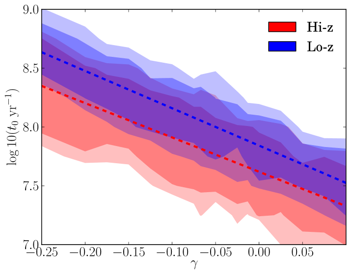
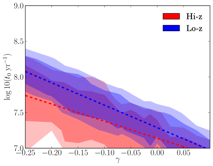
Table 4 summarizes the changes in best-fit parameters as a function of redshift. Interestingly, these values change somewhat: as structure continues to build, models with increasingly higher bias values are preferred. The fact that the best-fit values change demonstrates that the passive evolution of an increased clustering signal within a given model is not sufficient; rather, this redshift evolution introduces additional constraints that we can use to select the most appropriate model. Nevertheless, the results are consistent with no redshift evolution. The results of White et al. (2012) also suggest that redshift evolution is minimal. Extending the clustering measurements to a larger redshift range could provide important constraints on the properties of quasar hosts.

Appendix C Bias as a function of luminosity

Figure 12.— The best-fit parameter $s_{0}$ for the two-point correlation function in the form $\xi(s)=\quantity(s/s_{0})^{-2}$ as a function of power-law index $\gamma$ from Eqn. (3) for the lightbulb and exponential cases using a fiducial (solid) and low-luminosity (dashed) luminosity selection. The gray shaded region shows the BOSS measurement for the fiducial luminosity cut. For the low-luminosity quasars, we see opposite trends for the two models. For the lightbulb, more negative values of $\gamma$ mean that dimmer quasars have longer lifetimes, which combined with abundance matching implies they have more massive hosts. They therefore have larger values of $s_{0}$ compared to more positive values of $\gamma$. In the exponential case, larger values of $\gamma$ show more clustering because the bright quasars are longer lived, and are more likely to be included in the low-luminosity cuts while they are below their peak luminosity. Since they are abundance matched to more massive, highly clustered hosts, this leads to the behavior seen. See the text for further discussion.

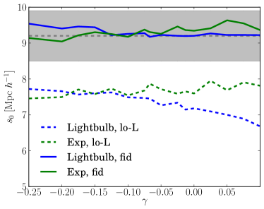
We can also examine the dependence of bias as a function of quasar luminosity. In the preceding analysis, we looked at the fiducial luminosity selection of the BOSS measurements for clustering, $-25\geq M_{i}\geq-27$. In order to break the degeneracy in Fig. 4, we explored the implications of measuring the clustering of quasars with different luminosity cuts. We examined a high-luminosity cut $M_{i}\leq-27$, and a low-luminosity cut $-23\geq M_{i}\geq-25$. Unfortunately, since the simulation volumes are only 1 ($h^{-1}$ Gpc)³, there are an insufficient number ($\sim$400) of high-luminosity objects to constrain the two-point correlation function.

When fitting the functional form of the two-point correlation function, a power law is used:

$$\xi(s)=\quantity(\frac{s}{s_{0}})^{\beta}.$$ (C1)

Fits the function are made for cases where the exponent $\beta$ is allowed to vary, and others with a fixed value of $\beta=-2$ as in White et al. (2012). In both cases, the clustering length $s_{0}$ increases for larger values of the bias. To fit the best parameters, the parameters $s_{0}$ and $\beta$ that minimized the $\chi^{2}=\delta^{\mathrm{T}}C^{-1}\delta$ value were found, where $\delta$ is defined as the difference between the average $\xi(s)$ and the functional form and $C$ is the covariance matrix, calculated in the same way as in Sec. 3.2. These fits were made for the best-fit models defined in Eqn. (20) using the values in Table 4.

Figure 12 shows the value of the correlation length fits $s_{0}$ for the fiducial luminosity cut $-25\geq M_{i}\geq-27$ (solid lines) and the low-luminosity cut $-23\geq M_{i}\geq-25$ (dashed lines) for the lightbulb and exponential models. The data are somewhat noisy, owing to the comparatively large shot-noise error in the correlation function measurement. However, there does seem to be a trend emerging: in the lightbulb case, for more negative values of $\gamma$, the bias is larger, with the opposite trend for the exponential case. In the lightbulb case, this can be explained by noting, as in Sec. 3.2, that in abundance matching longer lifetimes lead to a larger bias in the host halos. For negative values of $\gamma$, less luminous quasars have longer lifetimes. Subsequently these quasars are being hosted in more massive halos. This means the clustering is stronger for large negative values of $\gamma$, implying a larger value of $s_{0}$.

In the exponential case, the opposite trend is observed due to the presence of high-$L_{\mathrm{peak}}$ interlopers. For positive values of $\gamma$, brighter quasars have longer lifetimes, and are more likely to be included in the low-luminosity selection. Since these hosts are abundance matched to occupy more massive, more clustered halo hosts, this leads to a stronger clustering signal, and a larger value of $s_{0}$. The evolution is not as strong as in the lightbulb case, however. In principle, the clustering measurement in different luminosity ranges could help break the degeneracy of best-fit models.

Unfortunately, in practice this type of measurement might be difficult to actually make. The change in bias between the extreme values of $\gamma$ is not very significant, and the measurement is very noisy. The shaded gray region in Figure 12 shows the current 1$\sigma$ bounds from the BOSS measurement, which has a larger spread than the variation in $s_{0}$ as a function of $\gamma$. Nevertheless, this ratio is a possible way to break the degeneracy between the different models.

References

- Boyle et al. (2000) Boyle, B. J., Shanks, T., Croom, S. M., et al. 2000, MNRAS, 317, 1014
- Cen & Safarzadeh (2015) Cen, R., & Safarzadeh, M. 2015, ApJ, 798, L38
- Compostella et al. (2013) Compostella, M., Cantalupo, S., & Porciani, C. 2013, MNRAS, 435, 3169
- Compostella et al. (2014) —. 2014, MNRAS, 445, 4186
- Conroy & White (2013) Conroy, C., & White, M. 2013, ApJ, 762, 70
- Courbin et al. (2012) Courbin, F., Faure, C., Djorgovski, S. G., et al. 2012, A&A, 540, A36
- Croom et al. (2005) Croom, S. M., Boyle, B. J., Shanks, T., et al. 2005, MNRAS, 356, 415
- Croton (2009) Croton, D. J. 2009, MNRAS, 394, 1109
- Dawson et al. (2013) Dawson, K. S., Schlegel, D. J., Ahn, C. P., et al. 2013, AJ, 145, 10
- Di Matteo et al. (2012) Di Matteo, T., Khandai, N., DeGraf, C., et al. 2012, ApJ, 745, L29
- Dixon & Furlanetto (2009) Dixon, K. L., & Furlanetto, S. R. 2009, ApJ, 706, 970
- Dixon et al. (2014) Dixon, K. L., Furlanetto, S. R., & Mesinger, A. 2014, MNRAS, 440, 987
- Eddington (1926) Eddington, A. S. 1926, The Internal Constitution of the Stars (Cambridge: Cambridge University Press)
- Feng et al. (2014) Feng, Y., Di Matteo, T., Croft, R., & Khandai, N. 2014, MNRAS, 440, 1865
- Flesch (2015) Flesch, E. W. 2015, PASA, 32, 10
- Furlanetto & Oh (2008) Furlanetto, S. R., & Oh, S. P. 2008, ApJ, 681, 1
- Furlanetto & Stoever (2010) Furlanetto, S. R., & Stoever, S. J. 2010, MNRAS, 404, 1869
- Glikman et al. (2011) Glikman, E., Djorgovski, S. G., Stern, D., et al. 2011, ApJ, 728, L26
- Gunn & Peterson (1965) Gunn, J. E., & Peterson, B. A. 1965, ApJ, 142, 1633
- Hearin et al. (2013) Hearin, A. P., Zentner, A. R., Berlind, A. A., & Newman, J. A. 2013, MNRAS, 433, 659
- Hinshaw et al. (2013) Hinshaw, G., Larson, D., Komatsu, E., et al. 2013, ApJS, 208, 19
- Hopkins & Hernquist (2009) Hopkins, P. F., & Hernquist, L. 2009, ApJ, 698, 1550
- Hopkins et al. (2006) Hopkins, P. F., Hernquist, L., Cox, T. J., et al. 2006, ApJS, 163, 1
- Hopkins et al. (2008) Hopkins, P. F., Hernquist, L., Cox, T. J., & Kereš, D. 2008, ApJS, 175, 356
- Hopkins et al. (2007) Hopkins, P. F., Richards, G. T., & Hernquist, L. 2007, ApJ, 654, 731
- Ikeda et al. (2011) Ikeda, H., Nagao, T., Matsuoka, K., et al. 2011, ApJ, 728, L25
- Ikeda et al. (2012) —. 2012, ApJ, 756, 160
- Jakobsen et al. (1994) Jakobsen, P., Boksenberg, A., Deharveng, J. M., et al. 1994, Nature, 370, 35
- Jeeson-Daniel et al. (2014) Jeeson-Daniel, A., Ciardi, B., & Graziani, L. 2014, MNRAS, 443, 2722
- Kashikawa et al. (2015) Kashikawa, N., Ishizaki, Y., Willott, C. J., et al. 2015, ApJ, 798, 28
- Kaurov & Gnedin (2014) Kaurov, A. A., & Gnedin, N. Y. 2014, ApJ, 787, 146
- Lee et al. (2013) Lee, K.-G., Bailey, S., Bartsch, L. E., et al. 2013, AJ, 145, 69
- Lidz et al. (2006) Lidz, A., Hopkins, P. F., Cox, T. J., Hernquist, L., & Robertson, B. 2006, ApJ, 641, 41
- Lusso et al. (2015) Lusso, E., Worseck, G., Hennawi, J. F., et al. 2015, MNRAS, 449, 4204
- Madau et al. (1999) Madau, P., Haardt, F., & Rees, M. J. 1999, ApJ, 514, 648
- Martini (2004) Martini, P. 2004, Coevolution of Black Holes and Galaxies, 169
- Martini & Weinberg (2001) Martini, P., & Weinberg, D. H. 2001, ApJ, 547, 12
- Masters et al. (2012) Masters, D., Capak, P., Salvato, M., et al. 2012, ApJ, 755, 169
- McGreer et al. (2013) McGreer, I. D., Jiang, L., Fan, X., et al. 2013, ApJ, 768, 105
- McQuinn et al. (2011) McQuinn, M., Hernquist, L., Lidz, A., & Zaldarriaga, M. 2011, MNRAS, 415, 977
- McQuinn et al. (2009) McQuinn, M., Lidz, A., Zaldarriaga, M., et al. 2009, ApJ, 694, 842
- Osmer (2004) Osmer, P. S. 2004, Coevolution of Black Holes and Galaxies, 324
- Outram et al. (2003) Outram, P. J., Hoyle, F., Shanks, T., et al. 2003, MNRAS, 342, 483
- Porciani et al. (2004) Porciani, C., Magliocchetti, M., & Norberg, P. 2004, MNRAS, 355, 1010
- Porciani & Norberg (2006) Porciani, C., & Norberg, P. 2006, MNRAS, 371, 1824
- Raičević & Theuns (2011) Raičević, M., & Theuns, T. 2011, MNRAS, 412, L16
- Reimers et al. (1997) Reimers, D., Kohler, S., Wisotzki, L., et al. 1997, A&A, 327, 890
- Richards et al. (2006) Richards, G. T., Strauss, M. A., Fan, X., et al. 2006, AJ, 131, 2766
- Richardson et al. (2012) Richardson, J., Zheng, Z., Chatterjee, S., Nagai, D., & Shen, Y. 2012, ApJ, 755, 30
- Ross et al. (2013) Ross, N. P., McGreer, I. D., White, M., et al. 2013, ApJ, 773, 14
- Salpeter (1964) Salpeter, E. E. 1964, ApJ, 140, 796
- Schlegel et al. (2011) Schlegel, D., Abdalla, F., Abraham, T., et al. 2011, ArXiv e-prints, arXiv:1106.1706
- Schmidt & Green (1983) Schmidt, M., & Green, R. F. 1983, ApJ, 269, 352
- Schmidt et al. (1995) Schmidt, M., Schneider, D. P., & Gunn, J. E. 1995, AJ, 110, 68
- Shang et al. (2011) Shang, Z., Brotherton, M. S., Wills, B. J., et al. 2011, ApJS, 196, 2
- Shen & Kelly (2012) Shen, Y., & Kelly, B. C. 2012, ApJ, 746, 169
- Shen et al. (2007) Shen, Y., Strauss, M. A., Oguri, M., et al. 2007, AJ, 133, 2222
- Shen et al. (2009) Shen, Y., Strauss, M. A., Ross, N. P., et al. 2009, ApJ, 697, 1656
- Shull (1979) Shull, J. M. 1979, ApJ, 234, 761
- Sijacki et al. (2015) Sijacki, D., Vogelsberger, M., Genel, S., et al. 2015, MNRAS, 452, 575
- Simha et al. (2012) Simha, V., Weinberg, D. H., Davé, R., et al. 2012, MNRAS, 423, 3458
- Slosar et al. (2013) Slosar, A., Iršič, V., Kirkby, D., et al. 2013, J. Cosmology Astropart. Phys, 4, 26
- Springel et al. (2005) Springel, V., Di Matteo, T., & Hernquist, L. 2005, MNRAS, 361, 776
- Stevans et al. (2014) Stevans, M. L., Shull, J. M., Danforth, C. W., & Tilton, E. M. 2014, ApJ, 794, 75
- Syphers & Shull (2014) Syphers, D., & Shull, J. M. 2014, ApJ, 784, 42
- Telfer et al. (2002) Telfer, R. C., Zheng, W., Kriss, G. A., & Davidsen, A. F. 2002, ApJ, 565, 773
- Thorne (1974) Thorne, K. S. 1974, ApJ, 191, 507
- Tinker et al. (2008) Tinker, J., Kravtsov, A. V., Klypin, A., et al. 2008, ApJ, 688, 709
- Trac & Cen (2007) Trac, H., & Cen, R. 2007, ApJ, 671, 1
- Trac et al. (2008) Trac, H., Cen, R., & Loeb, A. 2008, ApJ, 689, L81
- Trac et al. (2015) Trac, H., Cen, R., & Mansfield, P. 2015, ApJ, 813, 54
- Trac & Pen (2004) Trac, H., & Pen, U.-L. 2004, New A, 9, 443
- Valageas et al. (2011) Valageas, P., Clerc, N., Pacaud, F., & Pierre, M. 2011, A&A, 536, A95
- Warren et al. (1994) Warren, S. J., Hewett, P. C., & Osmer, P. S. 1994, ApJ, 421, 412
- White et al. (2010) White, M., Pope, A., Carlson, J., et al. 2010, ApJ, 713, 383
- White et al. (2012) White, M., Myers, A. D., Ross, N. P., et al. 2012, MNRAS, 424, 933
- Worseck et al. (2011) Worseck, G., Prochaska, J. X., McQuinn, M., et al. 2011, ApJ, 733, L24
- Wyithe & Loeb (2003) Wyithe, J. S. B., & Loeb, A. 2003, ApJ, 595, 614
- Yu & Lu (2004) Yu, Q., & Lu, Y. 2004, ApJ, 602, 603
- Yu & Tremaine (2002) Yu, Q., & Tremaine, S. 2002, MNRAS, 335, 965
- Zehavi et al. (2005) Zehavi, I., Zheng, Z., Weinberg, D. H., et al. 2005, ApJ, 630, 1
- Zheng et al. (2008) Zheng, W., Meiksin, A., Pifko, K., et al. 2008, ApJ, 686, 195