45678 \TOGvolume0 \TOGnumber0 \TOGarticleDOI1111111.2222222 \TOGprojectURL \TOGvideoURL \TOGdataURL \TOGcodeURL \pdfauthorC. Xian et al.
![[Uncaptioned image]](/html/1507.02800/assets/x1.png)
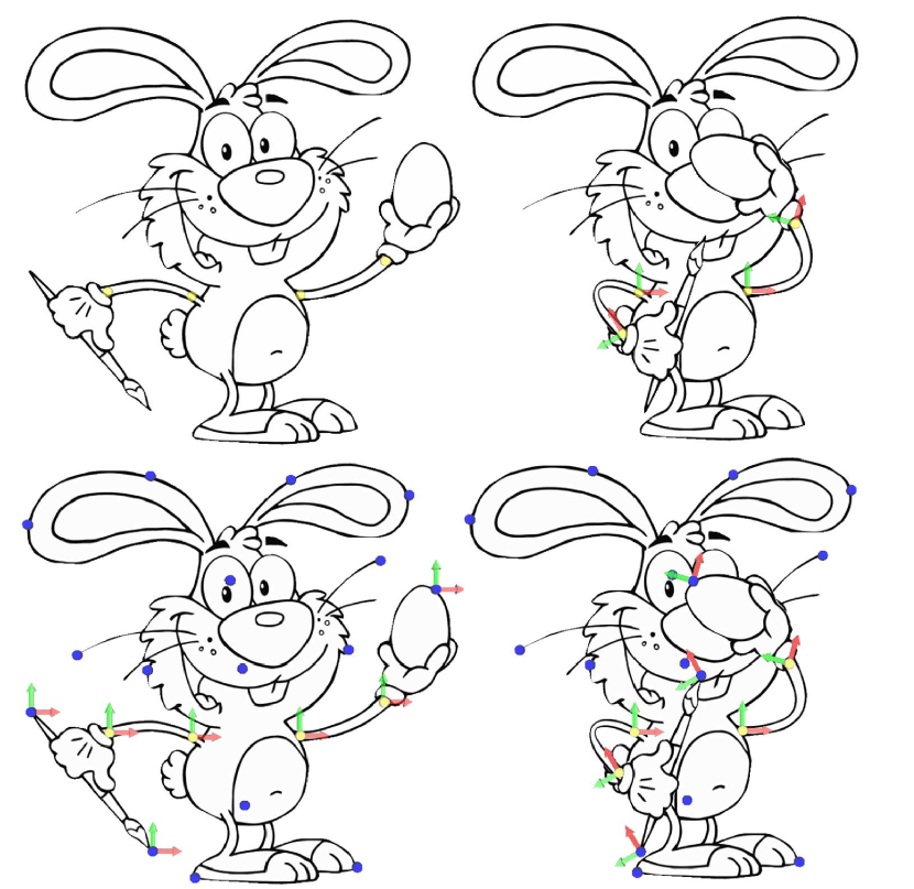
Deformation using meshfree -weighting. (a) Handle-driven deformation based on linear blending is an intuitive method for the interactive shape manipulation. (b) Artifacts caused by highly distorted triangles can be generated from the weights computed on an originally well-meshed domain. (c) We propose a meshfree framework to generate -continuous weights for linear blending based deformation. Our approach inherits the merits of mesh-dependent weighting schemes meanwhile bringing the weighting method to the resolution of infinity.
Meshfree -Weighting for Shape Deformation
Abstract
Handle-driven deformation based on linear blending is widely used in many applications because of its merits in intuitiveness, efficiency and easiness of implementation. We provide a meshfree method to compute the smooth weights of linear blending for shape deformation. The -continuity of weighting is guaranteed by the carefully formulated basis functions, with which the computation of weights is in a closed-form. Criteria to ensure the quality of deformation are preserved by the basis functions after decomposing the shape domain according to the Voronoi diagram of handles. The cost of inserting a new handle is only the time to evaluate the distances from the new handle to all sample points in the space of deformation. Moreover, a virtual handle insertion algorithm has been developed to allow users freely placing handles while preserving the criteria on weights. Experimental examples for real-time 2D/3D deformations are shown to demonstrate the effectiveness of this method.
keywords:
shape deformation, meshfree, closed-form formulation, linear blend skinningI.3.5Computer GraphicsComputational Geometry and Object ModelingGeometric algorithms, languages, and systems
1 Introduction
Shape deformation techniques have various applications in computer graphics for image manipulation, geometric modeling and animation. Compared with other deformation strategies, handle-driven methods outperform others as they are intuitive, effective and easy-to-implement in many different scenarios. Using handles, users can bind a shape with the handles and then manipulate their locations and orientations to drive the deformation of . Specifically, each handle with is defined as a local frame with its origin . After defining an affine transformation for each handle , the deformation of is realized by computing the new position of each point via a linear blending of affine transformations . The linear blending is weighted by fields associated with handles . Basically, to achieve an intuitive and high-quality deformation, the following criteria on the weights are demanded: smoothness, non-negativity, partition-of-unity, locality/sparsity, and no-local-maxima (see the analysis given in [\citenameJacobson et al. 2011]).
The recent advancement of technology focuses on computing weights of blending on a discrete form of domain (i.e., meshes are employed to determine piecewise linear fields of weights). Weights are computed on the mesh nodes via minimizing some discrete differential energies (e.g., biharmonic, triharmonic and quatraharmonic used in [\citenameJacobson et al. 2012b]). After incorporating the hard constraints according to the criteria on weights, the weights are determined on mesh nodes with the help of non-linear optimization. However, this is time-consuming. As a result, the insertion of new handles cannot be realized in real-time as new routines of non-linear optimization need to be taken. Moreover, the determined weights are mesh-dependent. For a symmetric shape to be deformed that is asymmetrically meshed, the computed weights for a handle located at the symmetric positions can rarely be symmetric. For poorly meshed computational domains, the artificial distortion caused by the elements of poor shape is more serious (as illustrated in Fig.Meshfree -Weighting for Shape Deformation). Although the artifacts can be reduced by increasing the density of meshes, this will further slow down the computation. Ideally, the distribution of weights should only be affected by the shape to be deformed and the locations of handles, which indicates mesh-independence. Existing mesh-independent approaches in literature for handle-driven deformation (e.g., [\citenameSingh and Fiume 1998, \citenameMilliron et al. 2002, \citenamevon Funck et al. 2006, \citenameSumner et al. 2007]) can only satisfy subsets of the demanded properties on weights. This motivates our work on investigating a new meshfree method to determine weights for shape deformation.
In this paper, we formulate the evaluation of weights in a closed-form so that the deformation framework based on this gains the benefit of flexibility – i.e., the response of inserting new handles is real-time. Specifically, the time cost of inserting a new handle is linear to the number of samples used to represent the domain of computation. The basis function formulated in this approach can guarantee the properties of smoothness, non-negativity, partition-of-unity, locality/sparsity, and no-local-maxima, all of which are necessary to ensure a deformation of high-quality.
The main results of our work are as follows:
-
•
We present a meshfree method to determine linear blending weights with -continuity for real-time deformation. The weights are formulated in a closed-form of basis functions centered at the handles (details are given in Section 3.1). After decomposing the region to be deformed by the Voronoi diagram of handles, aforementioned criteria of shape deformation are all ensured (see the analysis in Section 3.2).
-
•
A virtual handle insertion algorithm is proposed in Section 4 to guarantee the locality and sparsity of weighting so that a deformation interpolates the transformations defined on handles. The virtual handles are added to let the supporting region of the basis function defined on a handle not cover the origins of any other handles (see the algorithm in Section 4.1).
-
•
After constructing the Voronoi diagram of all handles (including user-input and virtual ones), its dual-graph gives a connectivity of the handles. We compute harmonic fields on the graph to determine the transformations of virtual handles according to the transformations specified on the user-input handles (see Section 4.2). It is found that the transformations determined in this way lead to a shape-aware deformation following the intention of user input.
With the help of a discrete implementation on point samples introduced in Section 5, an efficient and effective meshfree approach has been developed for handle-driven shape deformation. 2D/3D experimental results are shown in Section 6 to demonstrate the performance of our approach.
2 Related Work
Shape deformation is an important research area in image manipulation and geometric modeling. There are a large amount of existing approaches in literature. The purpose of this section is not for a comprehensive review. We only focus on discussing the handle-driven deformation approaches.
Mesh-based techniques for discrete geometry modeling and processing have been widely explored in the past decade. Typical approaches including variational surface deformation [\citenameBotsch and Kobbelt 2004], Poisson deformation [\citenameYu et al. 2004], Laplacian editing [\citenameSorkine et al. 2004] and other linear variational surface deformation approaches (see also the survey in [\citenameBotsch and Sorkine 2008]). Volumetric information and rigidity are also incorporated to enhance the shape-preservation in [\citenameIgarashi et al. 2005, \citenameBotsch et al. 2006, \citenameBotsch et al. 2007, \citenameSorkine and Alexa 2007]. One common drawback of these approaches is that the positions of vertices on a model need to be determined by solving a system of linear equations after every update of handles, which becomes a bottleneck of computation. A recent development in [\citenameJacobson et al. 2011, \citenameJacobson and Sorkine 2011, \citenameJacobson et al. 2012b] transfers the workload from online optimization to offline. Specifically, the weights corresponding to handles are computed on every vertex of a model before manipulating the handles (similar to [\citenameZayer et al. 2005]). The deformed shape is then evaluated by linear blending of transformations defined on handles. In [\citenameSumner et al. 2007], the handles are elements of a simplified mesh. Although this strategy is more efficient than the deformation methods based on online optimization, they still cannot avoid solving large linear systems, which slows down the response of deformation after inserting new handles. Moreover, the results of deformation are also suffered from the artificial distortions caused by the problems of meshes (e.g., too coarse meshes for a fine deformation, a mesh with ‘needle’ and ‘cap’ triangles, and the problem of symmetry). Our meshfree approach solves these problems by providing closed-form formulas to generate weights preserving all the demanded properties for producing deformations with high quality in real-time.
Another thread of researches for deformation focuses on mesh-independent approaches. Different handles are employed for shape manipulation. Points are used in [\citenameYoshizawa et al. 2002, \citenameSchaefer et al. 2006], and curves are employed as handles in [\citenameLazarus et al. 1994, \citenameSingh and Fiume 1998]. Grid-based deformation techniques in [\citenameSederberg and Parry 1986, \citenameLee et al. 1995] conduct the bivariate/trivariate cubic splines to realize deformations with -continuity. Users are allowed to move control points of the spline surfaces/solids to modify the embedded shapes, where the editing is indirect. Some approaches have been developed to extend this approach to provide the ability of direct editing (ref. [\citenameHsu et al. 1992, \citenameHu et al. 2001]). However, the computational domain is still limited to a simple topology (i.e., genus zero). An improvement of the grid-based techniques is introduced by Beier and Neely \shortciteBeier1992FIM to allow handles in the form of line segments by using the Shepard’s interpolation [\citenameShepard 1968]. Cage-based deformation (e.g., [\citenameJoshi et al. 2007, \citenameBen-Chen et al. 2009]) can be considered as a further generalization of grid-based deformation, where weights can be found by a closed-form in terms of the handles in [\citenameJu et al. 2005, \citenameLipman et al. 2008]. However, the construction of cages is usually not automatic and the manipulation on cages instead of a model itself is indirect.
Moving least square (MLS) strategy is employed in [\citenameSchaefer et al. 2006] for interpolating the similarity/rigid deformation at handle points. A closed-form solution is provided in their approach to determine the transformation matrix on every point in a MLS manner. The transformations in the whole domain need to be computed when any handle is moved. In other words, the deformation is globally affected by all handles – lack of sparsity. Different from this MLS approach, our approach belongs to the category of linear blending based deformation. When the property of sparsity is preserved on the weights, the deformation at a point is only affected by the nearby handles that is easier to be predicted by end-users. Moreover, the deformation determined by our approach is resolution independent, which is very important for image manipulation.
The work of generating weights for linear blending also relates to the research of scattered data interpolation, where radial basis functions (RBF) are widely used (e.g., [\citenameFloater and Iske 1996, \citenameBotsch and Kobbelt 2005]). In [\citenameBotsch and Kobbelt 2005], the deformation is governed by global RBFs that lead to a dense linear system to be solved. The weights determined by the dense (or global) data interpolation approaches lack of sparsity. Therefore, every point in the domain is changed when any handle is updated even if it is far away. Although the compactly supported radial basis functions (CSRBF) can help on introducing the sparsity (ref. [\citenameFloater and Iske 1996]), it does not provide closed-form formulas as our approach.
3 Meshfree Weighting
Following the linear blending formulation, the new position of a point is determined by the transformations defined on handles as111 is a homogenous matrix and is represented by homogeneous coordinate.
| (1) |
with being the scalar field of weights to be determined. The origin of a handle is denoted by . This linear blending based deformation is fast and easy-to-implement. However, carelessly assigned weights can lead to visible artifacts in results. Basically, a deformation with high quality must have the following properties:
-
•
Smoothness: The scalar field of weights must be smooth to avoid visual artifact (discontinuity) in both 2D and 3D deformations. We use compactly supported Bézier basis functions in our formulation, which lead to a weight field with -continuity.
-
•
Interpolation: The final transformation determined by the linear blending must interpolate the transformations at the handles. Specifically, the weight on a handle is one at its origin while basis functions centered at other handles give zero at this point. This is guaranteed by the locality and the sparsity in our formulation.
-
•
Consistency: When applying the same transformation on all handles, all points in must be consistently transformed by . This is enforced by the partition-of-unity property in our formulation. Another consistency requirement is about direction. The region influenced by a handle should not change in the inverse direction of the transformation assigned on the handle. We ensure this by the property of non-negativity.
-
•
Shape-awareness: This is a property more or less subjective. Basically, the intrinsic requirement on shape-awareness is to have deformations like stretching, bending and twisting an elastic solid, where the handles serve as pins. In our formulation, this is preserved by 1) having non-positive first derivative of basis functions and 2) letting all basis functions have similar support sizes. No-local-maxima on weights will prevent generating singularity (e.g., a point moves faster than all its neighbors) during deformation.
Our formulation below leads to -continuous weights preserving all these properties in deformations.
3.1 Formulation
Each handle is equipped with a compactly supported basis function with support size as , where is the location of and returns the intrinsic-distance (see Appendix A for the definition) between two points inside . The scalar field of the weights for is then defined as
| (2) |
which enforces the partition-of-unity.
To be shape-aware and interpolate handles, is chosen as a monotonically decreasing function with and (). A quintic polynomial is employed for the function so that the constraints for and -continuity at the boundary of the supporting regions can be satisfied. Specifically, we need
| (3) |
To ease the evaluation and analysis, each is represented as the -component (i.e., , ) of a 2D Bézier curve with degree- ()
| (4) |
where are the Bernstein polynomials. From the property of Bézier curves (ref. [\citenameFarin 2002]), we know that when . Letting and can satisfy these constraints at the endpoints (see Appendix B for more details). For the rest control points, we can simply assign them as or align them along the line uniformly.
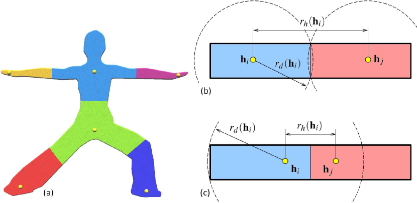
When the intrinsic-distance is used to generate the input parameter for the basis functions, linear blending based deformations driven by these basis functions behave in a shape-aware manner. Now the problem left is how to determine the support size of each basis function. As a basic requirement of handle-driven deformation based on linear blending, every point should be influenced by at least one handle. To be shape-aware, a point should be mostly affected by its closest handle in . Voronoi diagram sited at the origins of handles provides an intrinsic decomposition of according to these observations (see Fig.1(a)), where the intrinsic-distance in is used as the metric for generating the Voronoi diagram. We denote the cell that corresponds to by . Two metrics according to a handle can be defined as follows (see Fig.1(b) for an illustration):
-
•
The size of a Voronoi cell: ;
-
•
The separation to other sites: .
To let the basis function centered at cover all points in and to ensure the handle interpolation property, it should have
| (5) |
The support size can be with being specified by users as a shape factor. For most of the examples in this paper, is used. It is possible to have two handles too close to each other so that (see Fig.1(c) for an example). For solving such cases, we will use the virtual handle insertion algorithm (presented in Section 4).
3.2 Analysis and Discussion
We analyze the advantages of our formulation for the handle-driven deformation based on linear blending.
Non-negativity: so that . Moreover, when is ensured for all handles, every point in should be covered by at least one handle’s support. In other words, .
Partition-of-unity: This has been enforced by the formulation in Eq.(2). That is,
Locality/Sparsity: This is preserved by and the condition given in Eq.(5). The transformation at a point coincident with a handle is only determined by the handle itself. .
Smoothness: -continuity is preserved on the weights
determined by Eq.(2). First of all, the basis
function is -continuous for when is defined as a Bézier curve
in Eq.(4) with . Therefore,
is also -continuous when for any other . In the region that is only covered by the support of
, . Similarly, it is also a constant function
() in the region outside the support of . By
Eq.(3), it is not difficult to prove the
-continuity at the following two cases:
i) and ,
ii)
and ,
where both the first and second derivatives are zero.
No-local-maxima: The global maxima of a weight only happens at the origin of handle and the regions only covered by the support of . Besides, we also observe the phenomenon of no-local-maxima in all our experimental tests.
Closed-form: The weights at any point are evaluated in a closed-form (i.e., by Eq.(2)). This guarantees the flexibility of inserting new handles during the deformation in real-time.
Meshfree: As the evaluation of basis functions to determine the weights is only related to the intrinsic-distance from points to the origin of handles, the solution is independent of mesh quality and resolution. In the mesh-dependent solutions, elements with poor shape, which can occur after a drastic deformation step, must be optimized. Remeshing leads to another round of weights computation that could be time-consuming.
In short, our method preserves all the merits of prior methods for linear blending based deformation (e.g., [\citenameJacobson et al. 2011, \citenameJacobson and Sorkine 2011, \citenameJacobson et al. 2012b]) while introducing new benefits of flexibility and efficiency.
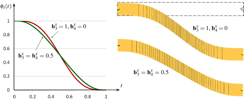
Besides the flexibility of inserting new handles during the deformation, we also provide users a method to change the behavior of handles by adjusting the shape of basis functions (i.e., ). For example, as shown in Fig.2, for the basis function built by a septic Bézier curve (), we can assign different values to and to obtain different shapes for to have different deformation behaviors. Basically, a ‘flat’ basis function (e.g., ) results in a deformation simulating hard materials while a more curved basis function (e.g., , ) makes the deformation soft. When using polynomials in higher orders, we have more degree-of-freedoms to change the shape of basis function. However, according to our experiments, septic polynomials are good enough in most of the cases.
The formulation of meshfree weighting also has some limitations. First, the interpolation property cannot be preserved when the distance between two handles are too close while the regions to be covered by either handle are large. Specifically, the interpolation of handles becomes an approximation when in Eq.(5) can NOT be satisfied. Second, for the region that is only covered by one handle, the transformation is consistent with the handle. Then, the deformation presented in this region is not shape-aware – i.e., the influence of handles does not decay while increasing the distance to the handle’s center. Both the problems will be solved by applying the virtual handle insertion approach presented in the following section.
4 Virtual Handle Insertion
A handle insertion algorithm is developed to enrich our meshfree weighting framework in the aspects of guaranteeing the handle interpolation property and improving the shape-awareness of deformation.
4.1 Insertion algorithm
When , we know that there are points in the voronoi cell whose distances to are larger than the minimal distance from to other handles.
Proposition 1 When , inserting new sites at the points with can reduce while keeping unchanged.
Proof.
First of all, the value of is not affected. When is the only point in with , it is obvious with . Define . After inserting a new site at , the points in become the member of . When all points with have been assigned to other voronoi cells, the value of reduces. On the other aspect, the distances from the newly inserted points to are which is greater than . ∎
Based on this proposition, we develop a greedy algorithm for handle insertion. Define as the set of handles and . When with , new handles are inserted to resolve this problem by reducing . The pseudo-code is described as Algorithm Virtual Handle Insertion.
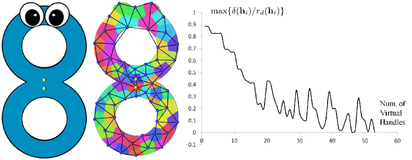
Remarks. From Proposition 1, we know that inserting new handles in a voronoi cell with can reduce the value of . However, inserting a new site can also affect the other handles (i.e., with ). In extreme cases, the original could be turned into . Then, new handles need to be added into .
Our virtual handle insertion algorithm can be considered as a variant of the farthest point sampling algorithm, which tends to tessellate a domain into a voronoi diagram with neighboring voronoi cells having similar sizes. The condition of is satisfied on all handles when this is the case. Our experimental tests also follow this observation (see Fig.3 for an example).
4.2 Transformation on Virtual Handles
A left problem is how to determine the transformation on virtual handles according to the user-specified transformations on real handles. Denote the set of real handles as and the set of virtual handles as . As aforementioned, the handles of have partitioned the given domain into a voronoi diagram . A dual graph of can be constructed by 1) using the sites of every voronoi cell as nodes and 2) linking the sites of every two neighboring voronoi cells by a straight line, which is a Delaunay graph [\citenameBerg et al. 2008]. We denote the Delaunay graph by and also use symbol to represent nodes in since each node is in fact a handle (real or virtual). The transformations of handles in are determined with the help of the Delaunay graph as follows.
-
•
For each handle in , a harmonic field is computed on to assign each handle a field value . Boundary conditions, and , are given to compute the harmonic field . If there are handles in , harmonic fields are determined on .
-
•
After converting the transformation of each handle into a rotation quaternion and a translation vector , the rotation and the translation on a virtual handle can be determined by
(6) with .
-
•
Finally, the quaternion and the translation determined on each virtual handle are converted back into a transformation matrix to be used in linear blending.
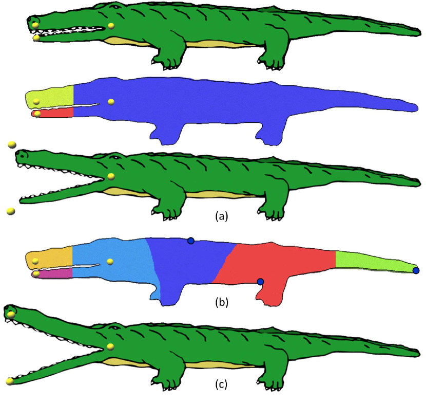
The transformation of virtual handles determined in this way brings in the effect of shape-awareness during the deformation. As illustrated in Figs.4 and 5, the deformation of whole domain driven by the transformations on handles (real and virtual) is very natural. The influence of a real handle decays when the distance to it increases.
5 Implementation Details
Similar to many other meshfree approaches, we sample the input domain to be deformed into a set of dense points . By searching -nearest-neighbors of each point, a graph spanning (in discrete form) can be established by using points in as nodes and adding links between neighboring points. Note that user specified handles should also be added into to construct the graph (i.e., ). The intrinsic-distance from any point to a handle is approximated by the distance between and the handle on the graph, which can be computed efficiently with the help of Dijkstra’s algorithm. Also, the voronoi diagram can be obtained by the Dijkstra’s algorithm with multiple sources on , where each sample is assigned to a voronoi cell. As the primitives used in the computation are points, the deformation approach can be easily generalized from 2D images to 3D solids. More examples can be found in the following section. To determine the weights on a general point that is not a sample in , a linear blending based on reciprocal distance weights [\citenameFloater and Reimers 2001] is employed to obtain the weight on from its -nearest-neighbors in . There are more sophisticated parameterization strategies in [\citenameFloater and Reimers 2001], which can also be applied here. With the help of this meshless parameterization, we can easily take an up-sampling step in the domain when the point set becomes sparse when applying a drastic deformation.
After using the virtual handle insertion algorithm to generate a set of new handles, harmonic fields are computed on a dual graph of to determine the transformations on virtual handles. By our boundary condition, all field values are non-negative when uniform Laplacian is employed [\citenameWardetzky et al. 2007]. In other words, the coefficients used in Eq.(6) are non-negative. Instead of solving a linear system to compute the harmonic field, we initially assign the field values on all real handles as one and the weights on all virtual handles are set as zero. Then we apply Laplacian operators to update their field values iteratively. The field values on virtual handles can be efficiently obtained after tens of iterations.
The point handles can be generalized to different types of handles (e.g., line segments and polygons, etc.). Specifically, each handle now becomes a set of points instead of a single point while all these points are equipped with the same transformation . The major change is the method to evaluate the intrinsic-distance from a query point to handles (e.g., line segments), which is the intrinsic-distance to ’s closest sample point on the handle. The rest of our approach will keep unchanged. Extreme case occurs when two line-segment handles have a common endpoint so that of these two handles becomes zero. There is no way to satisfy the condition of for handle interpolation. We therefore only approximate the transformations specified on handles. Specifically, the basis function is changed to a global Gaussian
| (7) |
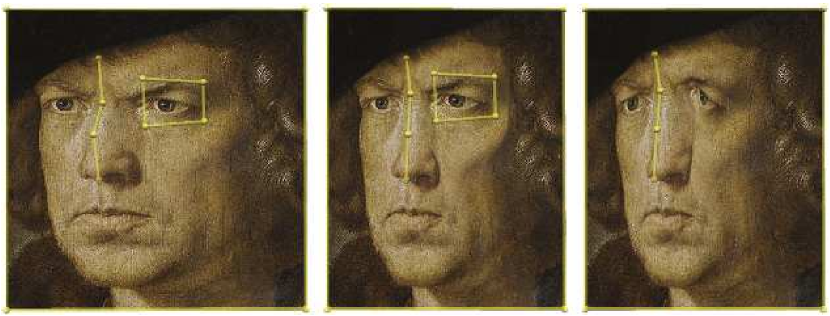
with being a constant to control the width of Gaussian. In our implementation, letting be works well in all tests. As some handles may have common endpoints, is changed to the minimal non-zero distance to other handles to exclude those connected handles. It is clear that the transformation at the position of a handle is commonly determined by all handles in although the influence of far away handles is trivial. On the other aspect, the smoothness of deformation is improved to . Cages can be formed by linking the segment handles into closed loops. For example when editing the portrait shown in Fig.6, the cage located at the boundary help resize the image. Moreover, the cage at the left eye fully controls the shape inside it and therefore preserves the salient feature.
6 Results
Our meshfree weighting method provides a compact tool to assign continuous weights for all points in the domain of deformation. With the help of sophisticated techniques for assigning transformations on the handles (e.g., the pseudo-edge method in [\citenameJacobson et al. 2011] or the optimization method in [\citenameJacobson et al. 2012a]), a natural user interface for shape deformation can be achieved.

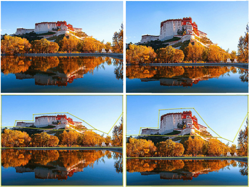
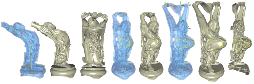
We have tested this approach in a variety of examples by using both the point and the segment handles. Figures Meshfree -Weighting for Shape Deformation, 4 and 5 have already demonstrated the functionality of point handles. Especially, in Fig.4, the scheme of virtual handles insertion guarantees the interpolation at real handles. Figure 5 illustrates the effectiveness of our method in determining transformations on virtual handles. The example of using segment handles to deform a portrait has been shown in Fig.6. Another example is given in Fig.7 to warp the the shape of palace. To obtain natural bending results, we can add rotations on handles by heuristic methods (e.g., the pseudo-edge [\citenameJacobson et al. 2011]). Another example is to demonstrate the performance of our approach in a symmetric deformation. When deforming a symmetric domain by adding symmetric transformations on symmetric handles, it is expected to get a symmetric result. This property is preserved by our formulation (see Fig.8).
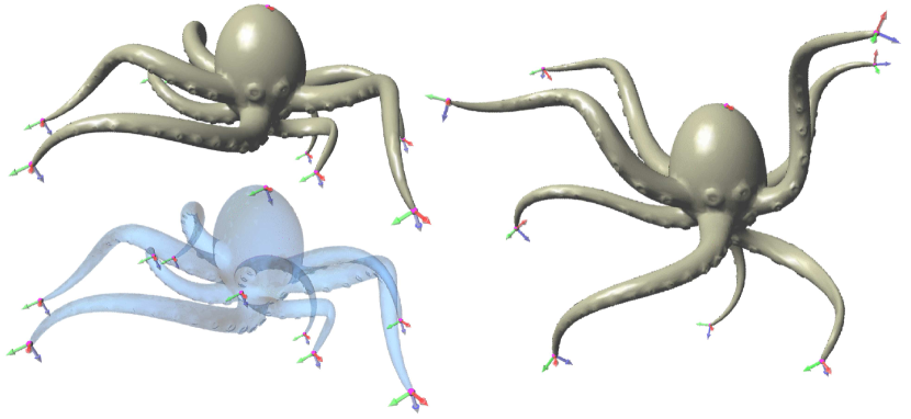
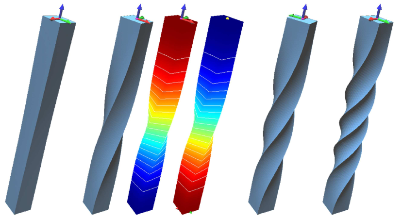
We also apply this method to deform 3D models. In these examples, the 3D models are represented by polygonal mesh surfaces. The weights computed by our approach are used in a linear blending way to determine the new positions of vertices. Note that, the space enclosed by a mesh surface need to be sampled into points with the help of voxelization technique (e.g., [\citenameSchwarz and Seidel 2010]) in order to evaluate the discrete intrinsic-distance in the domain to be deformed. Point handles are used to manipulate the flexible Octopus in Fig.9, where the interface of manipulation becomes user-friendly after employing the scheme of pseudo-edges to determine the transformation of point handles. Linear blending scheme is widely employed in the animation of skeletal models (e.g., [\citenameJacobson and Sorkine 2011, \citenameMagnenat-Thalmann et al. 1988]). The example shown in Fig.10 gives the performance of our approach in this scenario. 3D models with very complex topology (e.g., the Buddha model with internal truss structrues in Fig.11) that are hard to be meshed can be easily handled in our approach. When deformations with large rotation are applied (e.g., in Fig.12), a progressive deformation strategy can help generate satisfactory results.
| (sec.) | (sec.) | |||
|---|---|---|---|---|
| Gingerman | 2 (8) | 155,457 | 0.584 | 0.054 |
| Alligator | 3 (3) | 53,225 | 0.128 | 0.015 |
| Rabbit | 4 (15) | 22,972 | 0.128 | 0.015 |
| Portrait | 11 | 4,225 | 0.029 | 0.005 |
| Palace | 22 | 4,225 | 0.041 | 0.003 |
| Chinese | 2 | 4,076 | 0.008 | 0.001 |
| Octopus | 10 | 7,485 | 0.039 | 0.002 |
| Armadillo | 17 | 26,002 | 0.100 | 0.014 |
| Buddha | 4 | 236,661 | 0.302 | 0.051 |
| 20 | 236,661 | 0.834 | 0.160 | |
| Bar | 2 | 4,765 | 0.009 | 0.002 |
For prior mesh-based approaches, the numerical system must be solved once more when new handles are inserted. In our meshfree weighting formulation, the time cost of adding new handles is very trivial as the weights are determined in a closed-form. Table 1 lists the statistics of our approach on different examples. All the tests are conducted on a computer with Intel Core i7-3740QM CPU at 2.70GHz with 8GB memory, where our current implementation only uses a single-core. All results of deformation can be obtained at an interactive speed.
Discussion. When using the meshfree formulation presented in the paper to deform real 2D/3D objects, sample points are adopted as the medium for realizing the computation. The error-bound of computation on this discrete representation is guaranteed by the density of samples. However, during the process of a sequence of deformations, the density of points could be changed dramatically. In this sense, a dynamic up-sampling step should be integrated in the framework to preserve the error-bound of intrinsic-distance computation. The image editing applications can be implemented by using either the super-sampling technique or the texture mapping on a mesh. In our framework, the cost of weight evaluation is trivial after resampling. The bottleneck is the computation of intrinsic-distances on the sample points. Our current implementation is based on the Dijkstra’s algorithm. However, this shortest path problem with multiple sources can be computed in parallel on the system with many-cores [\citenameRong et al. 2011], which can result in a significant speedup and will be implemented in our future work.

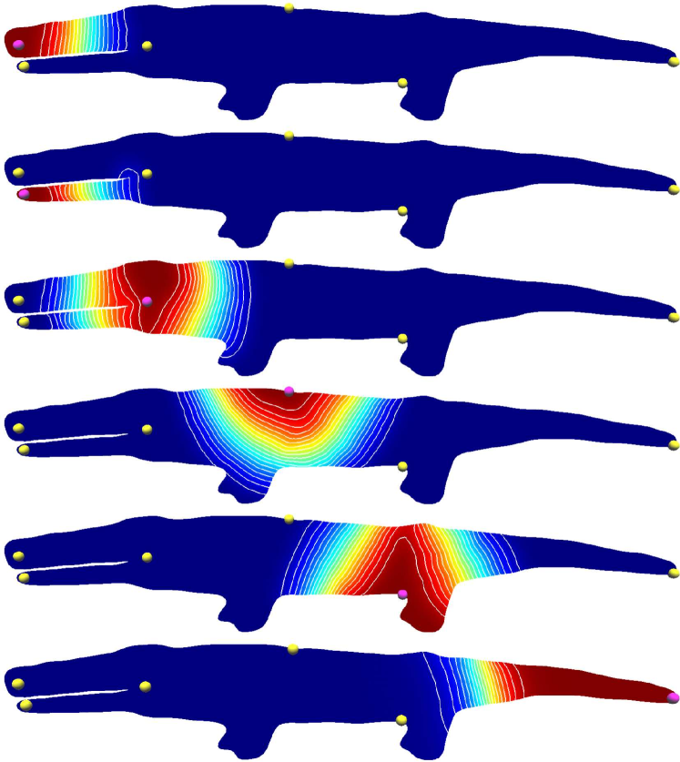
Our formulation gives global maximum at the positions of handles, which is very important to avoid the unintuitive behavior of deformations. For a shape-aware deformation, it is also demanded having no-local-maximum. This has been verified in our experimental tests. We check the topology of isocurves on the fields of weights (see Fig.13 for an example). If there is a closed loop formed by isocurves of at one place except the center of the handle , a local maximum is generated there. However, no such case is found in all our examples.
7 Conclusion
We present a method to determine weights of blending for shape deformation. Our formulation is meshfree and in a closed-form, which can be easily used in a variety of applications in 2D/3D deformations. Equipped with a virtual handle insertion algorithm, good properties of weights generated by prior mesh-based methods can all be preserved in this approach. A variety of examples have been shown to demonstrate the function of our approach.
Only linear blending deformations are tested in the paper. We plan to further extend the application of weights generated in this approach to more advanced skinning methods, such as dual quaternion [\citenameKavan et al. 2008], with which the blending of two rigid motions will result in a rigid motion. This is a very important property when the deformation of articulated characters is computed by the skinning methods. The deformations driven by linear blending are not always injective and therefore can generate the results with foldovers and self-intersection. Recently, some researches have been conducted in this direction to produce injective mappings (e.g., [\citenameAigerman and Lipman 2013, \citenameSchüller et al. 2013]), which are mainly mesh-based. In a function based formulation, the injectivity of a mapping can be checked by the sign of Jacobian. However, it is still not clear about how to resolve the problem when self-intersection is detected. This will be one of our future work.
References
- [\citenameAigerman and Lipman 2013] Aigerman, N., and Lipman, Y. 2013. Injective and bounded distortion mappings in 3D. ACM Trans. Graph. 32, 4, 106:1–106:14.
- [\citenameBeier and Neely 1992] Beier, T., and Neely, S. 1992. Feature-based image metamorphosis. SIGGRAPH Comput. Graph. 26, 2 (July), 35–42.
- [\citenameBen-Chen et al. 2009] Ben-Chen, M., Weber, O., and Gotsman, C. 2009. Variational harmonic maps for space deformation. ACM Trans. Graph. 28, 3 (July), 34:1–34:11.
- [\citenameBerg et al. 2008] Berg, M. d., Cheong, O., Kreveld, M. v., and Overmars, M. 2008. Computational Geometry: Algorithms and Applications, 3rd ed. Springer-Verlag TELOS, Santa Clara, CA, USA.
- [\citenameBotsch and Kobbelt 2004] Botsch, M., and Kobbelt, L. 2004. An intuitive framework for real-time freeform modeling. ACM Trans. Graph. 23, 3 (Aug.), 630–634.
- [\citenameBotsch and Kobbelt 2005] Botsch, M., and Kobbelt, L. 2005. Real-time shape editing using radial basis functions. Comput. Graph. Forum 24, 3, 611–621.
- [\citenameBotsch and Sorkine 2008] Botsch, M., and Sorkine, O. 2008. On linear variational surface deformation methods. IEEE Transactions on Visualization and Computer Graphics 14, 1 (Jan.), 213–230.
- [\citenameBotsch et al. 2006] Botsch, M., Pauly, M., Gross, M., and Kobbelt, L. 2006. Primo: Coupled prisms for intuitive surface modeling. In Proceedings of the Fourth Eurographics Symposium on Geometry Processing, Eurographics Association, SGP ’06, 11–20.
- [\citenameBotsch et al. 2007] Botsch, M., Pauly, M., Wicke, M., and Gross, M. H. 2007. Adaptive space deformations based on rigid cells. Comput. Graph. Forum 26, 3, 339–347.
- [\citenameFarin 2002] Farin, G. 2002. Curves and Surfaces for CAGD: A Practical Guide, 5th ed. Morgan Kaufmann Publishers Inc., San Francisco, CA, USA.
- [\citenameFloater and Iske 1996] Floater, M. S., and Iske, A. 1996. Multistep scattered data interpolation using compactly supported radial basis functions. Journal of Computational and Applied Mathematics 73, 1-2, 65–78.
- [\citenameFloater and Reimers 2001] Floater, M. S., and Reimers, M. 2001. Meshless parameterization and surface reconstruction. Computer Aided Geometric Design 18, 2, 77–92.
- [\citenameHsu et al. 1992] Hsu, W. M., Hughes, J. F., and Kaufman, H. 1992. Direct manipulation of free-form deformations. SIGGRAPH Comput. Graph. 26, 2 (July), 177–184.
- [\citenameHu et al. 2001] Hu, S.-M., Zhang, H., Tai, C.-L., and Sun, J.-G. 2001. Direct manipulation of ffd: efficient explicit solutions and decomposible multiple point constraints. The Visual Computer 17, 6, 370–379.
- [\citenameIgarashi et al. 2005] Igarashi, T., Moscovich, T., and Hughes, J. F. 2005. As-rigid-as-possible shape manipulation. ACM Trans. Graph. 24, 3 (July), 1134–1141.
- [\citenameJacobson and Sorkine 2011] Jacobson, A., and Sorkine, O. 2011. Stretchable and twistable bones for skeletal shape deformation. ACM Trans. Graph. 30, 6 (Dec.), 165:1–165:8.
- [\citenameJacobson et al. 2011] Jacobson, A., Baran, I., Popović, J., and Sorkine, O. 2011. Bounded biharmonic weights for real-time deformation. ACM Trans. Graph. 30, 4 (July), 78:1–78:8.
- [\citenameJacobson et al. 2012a] Jacobson, A., Baran, I., Kavan, L., Popović, J., and Sorkine, O. 2012. Fast automatic skinning transformations. ACM Trans. Graph. 31, 4, 77:1–77:10.
- [\citenameJacobson et al. 2012b] Jacobson, A., Weinkauf, T., and Sorkine, O. 2012. Smooth shape-aware functions with controlled extrema. Comp. Graph. Forum 31, 5 (Aug.), 1577–1586.
- [\citenameJoshi et al. 2007] Joshi, P., Meyer, M., DeRose, T., Green, B., and Sanocki, T. 2007. Harmonic coordinates for character articulation. ACM Trans. Graph. 26, 3 (July).
- [\citenameJu et al. 2005] Ju, T., Schaefer, S., and Warren, J. 2005. Mean value coordinates for closed triangular meshes. ACM Trans. Graph. 24, 3 (July), 561–566.
- [\citenameKavan et al. 2008] Kavan, L., Collins, S., Žára, J., and O’Sullivan, C. 2008. Geometric skinning with approximate dual quaternion blending. ACM Trans. Graph. 27, 4, 105:1–105:23.
- [\citenameLazarus et al. 1994] Lazarus, F., Coquillart, S., and Jancéne, P. 1994. Axial deformations: an intuitive deformation technique. Computer-Aided Design 26, 8, 607–613.
- [\citenameLee et al. 1995] Lee, S.-Y., Chwa, K.-Y., and Shin, S. Y. 1995. Image metamorphosis using snakes and free-form deformations. In Proceedings of the 22Nd Annual Conference on Computer Graphics and Interactive Techniques, ACM, SIGGRAPH ’95, 439–448.
- [\citenameLipman et al. 2008] Lipman, Y., Levin, D., and Cohen-Or, D. 2008. Green coordinates. ACM Trans. Graph. 27, 3 (Aug.), 78:1–78:10.
- [\citenameMagnenat-Thalmann et al. 1988] Magnenat-Thalmann, N., Laperrière, R., and Thalmann, D. 1988. Joint-dependent local deformations for hand animation and object grasping. In Proceedings on Graphics Interface ’88, 26–33.
- [\citenameMilliron et al. 2002] Milliron, T., Jensen, R. J., Barzel, R., and Finkelstein, A. 2002. A framework for geometric warps and deformations. ACM Trans. Graph. 21, 1 (Jan.), 20–51.
- [\citenameRong et al. 2011] Rong, G., Liu, Y., Wang, W., Yin, X., Gu, X. D., and Guo, X. 2011. Gpu-assisted computation of centroidal voronoi tessellation. IEEE Transactions on Visualization and Computer Graphics 17, 3, 345–356.
- [\citenameSchaefer et al. 2006] Schaefer, S., McPhail, T., and Warren, J. 2006. Image deformation using moving least squares. ACM Trans. Graph. 25, 3 (July), 533–540.
- [\citenameSchüller et al. 2013] Schüller, C., Kavan, L., Panozzo, D., and Sorkine-Hornung, O. 2013. Locally injective mappings. Computer Graphics Forum (proceedings of EUROGRAPHICS/ACM SIGGRAPH Symposium on Geometry Processing) 32, 5, 125–135.
- [\citenameSchwarz and Seidel 2010] Schwarz, M., and Seidel, H.-P. 2010. Fast parallel surface and solid voxelization on gpus. ACM Trans. Graph. 29, 6, 179:1–179:10.
- [\citenameSederberg and Parry 1986] Sederberg, T. W., and Parry, S. R. 1986. Free-form deformation of solid geometric models. SIGGRAPH Comput. Graph. 20, 4 (Aug.), 151–160.
- [\citenameShepard 1968] Shepard, D. 1968. A two-dimensional interpolation function for irregularly-spaced data. In Proceedings of the 1968 23rd ACM National Conference, ACM, 517–524.
- [\citenameSingh and Fiume 1998] Singh, K., and Fiume, E. 1998. Wires: A geometric deformation technique. In Proceedings of the 25th Annual Conference on Computer Graphics and Interactive Techniques, ACM, SIGGRAPH ’98, 405–414.
- [\citenameSorkine and Alexa 2007] Sorkine, O., and Alexa, M. 2007. As-rigid-as-possible surface modeling. In Proceedings of the Fifth Eurographics Symposium on Geometry Processing, Eurographics Association, SGP ’07, 109–116.
- [\citenameSorkine et al. 2004] Sorkine, O., Cohen-Or, D., Lipman, Y., Alexa, M., Rössl, C., and Seidel, H.-P. 2004. Laplacian surface editing. In Proceedings of the 2004 Eurographics/ACM SIGGRAPH Symposium on Geometry Processing, ACM, SGP ’04, 175–184.
- [\citenameSumner et al. 2007] Sumner, R. W., Schmid, J., and Pauly, M. 2007. Embedded deformation for shape manipulation. ACM Trans. Graph. 26, 3 (July).
- [\citenamevon Funck et al. 2006] von Funck, W., Theisel, H., and Seidel, H.-P. 2006. Vector field based shape deformations. ACM Trans. Graph. 25, 3 (July), 1118–1125.
- [\citenameWardetzky et al. 2007] Wardetzky, M., Mathur, S., Kälberer, F., and Grinspun, E. 2007. Discrete laplace operators: No free lunch. In Proceedings of the Fifth Eurographics Symposium on Geometry Processing, 33–37.
- [\citenameYoshizawa et al. 2002] Yoshizawa, S., Belyaev, A., and Seidel, H. P. 2002. A simple approach to interactive free-form shape deformations. In Proceedings of 10th Pacific Conference on Computer Graphics and Applications, 471–474.
- [\citenameYu et al. 2004] Yu, Y., Zhou, K., Xu, D., Shi, X., Bao, H., Guo, B., and Shum, H.-Y. 2004. Mesh editing with poisson-based gradient field manipulation. ACM Trans. Graph. 23, 3 (Aug.), 644–651.
- [\citenameZayer et al. 2005] Zayer, R., Rössl, C., Karni, Z., and Seidel, H.-P. 2005. Harmonic guidance for surface deformation. Comput. Graph. Forum 24, 3, 601–609.
Appendix A: Intrinsic-Distance
For a 2-manifold shape in 2D/3D Euclidean space, all points on the shape form a bounded domain . For any two points , if there exists a curve line connecting and , we define the intrinsic-distance of along the curve as
Then the intrinsic-distance of in is defined as
If there is no curve connecting and , that is the case they are not located in a connected region of . The intrinsic-distance is then defined as .
Sampling based intrinsic-distance. For a set of sampling points of , we can build a graph by using the sample points as nodes. We represent the shortest distance between and on as . If for any two points , we always have
the sampling is a distance-bounded sampling of .
The intrinsic-distance defined in this way has the following properties:
-
•
Existence: is always calculable once is determined, which is a curve segment in . Therefore, always exists for when and are located in the same connected region.
-
•
Uniqueness: is uniquely determined while the corresponding curves may be multiple.
-
•
Convergency: For any , there always exists an infinite sampling of – that is the sampling density . Since , we have
Appendix B: Endpoint Constraints
From the analysis in [\citenameFarin 2002], we know that
for a Bézier curve in -th order. And also
Incorporating the constraints in Eq.(3), we have
As we already need to let , it is not difficult to find that and satisfy all these constraints.