On Joint Estimation of Gaussian Graphical Models for Spatial and Temporal Data

Abstract

In this paper, we first propose a Bayesian neighborhood selection method to estimate Gaussian Graphical Models (GGMs). We show the graph selection consistency of this method in the sense that the posterior probability of the true model converges to one. When there are multiple groups of data available, instead of estimating the networks independently for each group, joint estimation of the networks may utilize the shared information among groups and lead to improved estimation for each individual network. Our method is extended to jointly estimate GGMs in multiple groups of data with complex structures, including spatial data, temporal data and data with both spatial and temporal structures. Markov random field (MRF) models are used to efficiently incorporate the complex data structures. We develop and implement an efficient algorithm for statistical inference that enables parallel computing. Simulation studies suggest that our approach achieves better accuracy in network estimation compared with methods not incorporating spatial and temporal dependencies when there are shared structures among the networks, and that it performs comparably well otherwise. Finally, we illustrate our method using the human brain gene expression microarray dataset, where the expression levels of genes are measured in different brain regions across multiple time periods.

Keywords: Spatial and Temporal Data; Gaussian Graphical Model; Neighborhood Selection; Bayesian Variable Selection; Markov Random Field.

1 Introduction

The analysis of biological networks, including protein-protein interaction networks (PPI), biological pathways, transcriptional regulatory networks and gene co-expression networks, has led to numerous advances in the understanding of the organization and functionality of biological systems e.g., Kanehisa & Goto 2000; Shen-Orr et al. 2002; Rual et al. 2005; Zhang & Horvath 2005. The work presented in this paper was motivated from the analysis of the human brain gene expression microarray data, where the expression levels of genes were measured in numerous spatial loci, which represent different brain regions, during different time periods of brain development (Kang et al., 2011). Although these data offer rich information on the network information among genes, only naive methods have been used for network inference. For example, Kang et al. (2011) pooled all the data from different spatial regions and time periods to construct a single gene network. However, only a limited number of data points are available for a specific region and time period, making region- and time- specific inference challenging.

Our aim here is to develop sound statistical methods to characterize the changes in the networks across time periods and brain regions, as well as the common network edges that are shared. This is achieved through a joint modeling framework to infer individual graphs for each brain region in each time period, where the degrees of spatial and temporal similarity are learnt adaptively from the data. Our proposed joint modeling framework may better capture the edges that are shared among graphs, and also allow the graphs to differ across brain regions and time periods.

We represent the biological network with a graph $G=(V,E)$ consisting of vertices $V=\{1,...,p\}$ and edges $E\subset V\times V$. In this paper, we focus on conditionally independent graphs, where $(i,j)\in E$ if and only if node $i$ and node $j$ are not conditionally independent given all the other nodes. Gaussian graphical models (GGMs) have been proven among the best to infer conditionally independent graphs. In GGM, the $p$-dimensional $X=(X_{1},\ldots,X_{p})$ is assumed to follow a multivariate Gaussian distribution $\mathcal{N}(\mu,\Sigma)$. Denote $\Theta=\Sigma^{-1}$ the precision matrix. It can be shown that the conditional independence of $X_{i}$ and $X_{j}$ is equivalent to $\Theta_{ij}\neq 0$: $X_{i}\perp\!\!\!\perp X_{j}\mid X_{V\backslash\{i,j\}}\Longleftrightarrow\Theta_{ij}=0$. In GGM, estimating the conditional independence graph is equivalent to estimating the non-zero entries in $\Theta$. Various approaches have been proposed to estimate the graph (Meinshausen & Bühlmann, 2006; Yuan & Lin, 2007; Friedman et al., 2008; Cai et al., 2011; Dobra et al., 2011; Wang et al., 2012; Orchard et al., 2013). Among these methods, Friedman et al. (2008) developed a fast and simple algorithm, named the graphical lasso (glasso), using a coordinate descent procedure for the lasso. They considered optimizing the penalized likelihood, with $\ell_{1}$ penalty on the precision matrix. As extensions of glasso, several approaches have been proposed to jointly estimate GGMs in multiple groups of data. Guo et al. (2011) expressed the elements of the precision matrix for each group as a product of binary common factors and group-specific values. They incorporated an $\ell_{1}$ penalty on the common factors, to encourage shared sparse structure, and another $\ell_{1}$ penalty on the group-specific values, to allow edges included in the shared structure to be set to zero for specific groups. Danaher et al. (2014) extended glasso more directly by extending the $\ell_{1}$ penalty for each precision matrix with additional penalty functions that encourage shared structure. They proposed two possible choices of penalty functions: 1. Fused lasso penalty that penalizes the difference of the precision matrices, which encourages common values among the precision matrices; 2. Group lasso penalty. Chun et al. (2014) proposed a class of non-convex penalties for more flexible joint sparsity constraints. As an alternative to the penalized methods, Peterson et al. (2014) proposed a Bayesian approach. They formulated the model in the $G$-Wishart prior framework and modeled the similarity of multiple graphs through a Markov Random Field (MRF) prior. However, their approach is only applicable when the graph size is small ($\sim 20$) and the number of groups is also small ($\sim 5$).

In this paper, we formulate the model in a Bayesian variable selection framework (George & McCulloch, 1993, 1997). Meinshausen & Bühlmann (2006) proposed a neighborhood selection procedure for estimating GGMs, where the neighborhood of node $i$ was selected by regressing on all the other nodes. Intuitively, our approach is the Bayesian analog of the neighborhood selection procedure. Our framework is applicable to the estimation of both single graph and multiple graphs. For the joint estimation of multiple graphs, we incorporate the MRF model. Compared with Peterson et al. (2014), we use a different MRF model and a different inferential procedure. One advantage of our approach is that it can naturally model complex data structures, such as spatial data, temporal data and data with both spatial and temporal structures. Another advantage is the computational efficiency. For the estimation of a single graph with $100$ nodes (the typical size of biological pathways is around that range), the computational time on a laptop is $\sim 30$ seconds for $1,000$ iterations of Gibbs sampling, which is $\sim 3$-folds faster than Bayesian Graphical Lasso, which implements a highly efficient block Gibbs sampler and is among the fastest algorithms for estimating GGMs in the Bayesian framework (Wang et al., 2012). For multiple graphs, the computational time increases roughly linear with the number of graphs. Our procedure also enables parallel computing and the computational time can be substantially reduced if multicore processors are available. For single graph estimation, we show the graph selection consistency of the proposed method in the sense that the posterior probability of the true model converges to one.

The rest of the paper is organized as follows. We introduce the Bayesian neighborhood selection procedure for single graph and the extension to multiple graphs in Section 2. Model selection is discussed in Section 3. The theoretical properties are presented in Section 4. The simulation results are demonstrated in Section 5 and the application to the human brain gene expression microarray dataset is presented in Section 6. We conclude the paper with a brief summary in Section 7.

2 Statistical Model and Methods

2.1 The Bayesian Neighborhood Selection Procedure

We first consider estimating the graph structure when there is only one group of data. Consider the $p$-dimensional multivariate normal random variable $X\sim\mathcal{N}(\mu,\Sigma)$. We further assume that $X$ is centered and $X\sim\mathcal{N}(0,\Sigma)$. Let $\Theta=\Sigma^{-1}$ denote the precision matrix. Let the $n\times p$ matrix $\mathbf{X}=(\mathbf{X}_{1},\ldots,\mathbf{X}_{p})$ contain $n$ independent observations of $X$. For $A\subseteq\{1,\ldots,p\}$, define $\mathbf{X}_{A}=(\mathbf{X}_{j},j\in A)$. Let $\Gamma_{i}$ denote the subset of $\{1,\ldots,p\}$, excluding the $i$th entry only. For any square matrix $C$, let $C_{i\Gamma_{i}}$ denote the $i$th row, excluding the $i$th element in that row. Consider estimating the neighborhood of node $i$. It is well known that the following conditional distribution holds:

$$\mathbf{X}_{i}\mid\mathbf{X}_{\Gamma_{i}}\sim\mathcal{N}(-\mathbf{X}_{\Gamma_{i}}\Theta_{i\Gamma_{i}}^{T}\Theta_{ii}^{-1},\Theta_{ii}^{-1}\bm{I}),$$ (1)

where $\bm{I}$ is the $n\times n$ identity matrix, $\Theta_{ii}$ is a scalar and finding the neighborhood of $X_{i}$ is equivalent to estimating the non-zero coefficients in the regression of $X_{i}$ on $X_{\Gamma_{i}}$. Let $\bm{\beta}$ and $\bm{\gamma}$ be matrices of dimension $p\times p$, where $\bm{\beta}_{i\Gamma_{i}}=-\Theta_{ii}^{-1}\Theta_{i\Gamma_{i}}$ and $\bm{\gamma}$ is the binary latent state matrix. The diagonal elements in $\bm{\beta}$ and $\bm{\gamma}$ are not assigned values. Conditioning on $\gamma_{ij}$, $\beta_{ij}$ is assumed to follow a normal mixture distribution (George & McCulloch, 1993, 1997):

$$\text{ }\beta_{ij}\mid\gamma_{ij}\sim(1-\gamma_{ij})\mathcal{N}(0,\tau_{i0}^{2})+\gamma_{ij}\mathcal{N}(0,\tau_{i1}^{2}),\text{ for }j\in\Gamma_{i},\\$$

where $\tau_{i0}/\tau_{i1}=\delta$ and $0<\delta<1$. The prior on $\gamma_{ij}$ is Bernoulli:

$$p(\gamma_{ij}=1)=1-p(\gamma_{ij}=0)=q.$$

$\delta$, $\tau_{i1}$ and $q$ are prefixed hyperparameters and are discussed in the Supplementary Materials. The off-diagonal entries in $\bm{\gamma}$ represent the presence or absence of the edges, which is the goal of our inference.

Let $\bm{\sigma}=(\sigma_{1},\ldots,\sigma_{p})$, where $\sigma_{i}^{2}=\Theta_{ii}^{-1}$. The inverse gamma (IG) conjugate prior is assumed for $\sigma_{i}^{2}$:

$$\sigma_{i}^{2}\mid\bm{\gamma}\sim IG(\nu_{i}/2,\lambda\nu_{i}/2).$$

In this paper, we assume that $\nu_{i}=0$ and the IG prior reduces to a flat prior (Li & Zhang, 2010).

For each node, we perform the Bayesian procedure to select the neighbors of that node. The precision matrix $\Theta$ is symmetric. If we let $\bm{\beta}_{i\Gamma_{i}}=-\Theta_{i\Gamma_{i}}$ instead of $-\Theta_{ii}^{-1}\Theta_{i\Gamma_{i}}$, the symmetric constraint can be satisfied by forcing $\bm{\beta}$ to be symmetric. However, this will lead to substantial loss in computational efficiency since the elements in $\bm{\beta}$ have to be updated one at a time, instead of one row at a time. Our simulation results suggest that the performance of the two models is comparable, whether or not the constraint on $\bm{\beta}$ is assumed (data not shown). Therefore, we do not constrain $\bm{\beta}$ in our inference. The selected neighborhood should be symmetric (the support of $\Theta$ is symmetric). Meinshausen & Bühlmann (2006) suggested using an or/and rule after their neighborhood selection procedure for each node. In our Bayesian procedure, the symmetric constrain can be incorporated naturally when sampling $\bm{\gamma}$ by setting $\gamma_{ij}=\gamma_{ji}$ for $j\neq i$. When there is no constraint assumed, the Bayesian procedure can be performed independently for each node.

2.2 Extension to mutiple graphs

When there is similarity shared among multiple graphs, jointly estimating multiple graphs can improve inference. We propose to jointly estimate multiple graphs by specifying a Markov Random Field (MRF) prior on the latent states. Our model can naturally incorporate complex data structures, such as spatial data, temporal data and data with both spatial and temporal structures. Consider jointly estimating multiple graphs for data with both spatial and temporal structures. Denote $B$ the set of spatial loci and $T$ the set of time points. Our proposed model can be naturally implemented when there is missing data, i.e. no data points taken in certain locus at certain time point. For now, we assume that there is no missing data. The latent states for the whole dataset are represented by a $|B|\times|T|\times p\times p$ array $\bm{\gamma}$, where $|$ $|$ denotes the cardinality of a set. Let $\bm{\gamma}_{bt\cdot\cdot}$ denote the latent state matrix for locus $b$ at time $t$. In the real data example, $b$ is a categorical variable representing the brain region and $t$ is a discrete variable that represents the time period during brain development. Same as that in Section 2.1, the diagonal entries in $\bm{\gamma}_{bt\cdot\cdot}$ are not assigned values.

Consider estimating the neighborhood of node $i$. Let $\gamma_{btij}$ denote the latent state for node $j\in\Gamma_{i}$ in locus $b$ at time $t$. Denote $\bm{\gamma_{\cdot\cdot ij}}=\{\gamma_{btij}:\forall b\in B,\forall t\in T\}$, $E^{s}_{ij}=\{(\gamma_{ijbt},\gamma_{ijb^{\prime}t^{\prime}}):b\neq b^{\prime}\text{, }t=t^{\prime}\}$ and $E^{t}_{ij}=\{(\gamma_{btij},\gamma_{b^{\prime}t^{\prime}ij}):b=b^{\prime}\text{ and }|t-t^{\prime}|=1\}$. Here $E^{s}_{ij}$ contain all the pairs capturing spatial similarity and $E^{t}_{ij}$ contain all the pairs capturing temporal dependency between adjacent time periods. We do not consider the direction of the pairs: $(\gamma_{ijbt},\gamma_{ijb^{\prime}t^{\prime}})$ and $(\gamma_{ijb^{\prime}t^{\prime}},\gamma_{ijbt})$ are the same. Let $I_{1}(\cdot)$ and $I_{0}(\cdot)$ represent the indicator functions of $1$ and $0$, respectively. The prior for $\bm{\gamma_{\cdot\cdot ij}}$ is specified by a pairwise interaction MRF model (Besag, 1986; Lin et al., 2015):

$$\begin{split}p(\bm{\gamma}_{\cdot\cdot ij}\mid\bm{\Phi})\propto\exp&\Bigg{\{}\eta_{1}\sum_{b\in B,t\in T}I_{1}(\gamma_{ijbt})+\\ &\eta_{s}\sum_{E^{s}_{ij}}\Big{[}I_{0}(\gamma_{btij})I_{0}(\gamma_{b^{\prime}t^{\prime}ij})+I_{1}(\gamma_{btij})I_{1}(\gamma_{b^{\prime}t^{\prime}ij})\Big{]}+\\ &\eta_{t}\sum_{E^{t}_{ij}}\Big{[}I_{0}(\gamma_{btij})I_{0}(\gamma_{b^{\prime}t^{\prime}ij})+I_{1}(\gamma_{btij})I_{1}(\gamma_{b^{\prime}t^{\prime}ij})\Big{]}\Bigg{\}},\end{split}$$ (2)

and conditional independence is assumed:

$$p(\bm{\gamma}\mid\bm{\Phi})=\prod_{i}\prod_{j\in\Gamma_{i}}p(\bm{\gamma}_{\cdot\cdot ij}\mid\bm{\Phi}),$$ (3)

where $\bm{\Phi}=\{\eta_{1},\eta_{s},\eta_{t}\}$ are set to be the same for all $i$ and $j$. $\eta_{1}\in\mathbb{R}$ and when there is no interaction terms, $1/(1+\exp(-\eta_{1}))$ corresponds to $q$ in the Bernoulli prior. $\eta_{s}\in\mathbb{R}$ represents the magnitude of spatial similarity and $\eta_{t}\in\mathbb{R}$ represents the magnitude of temporal similarity. In the simulation and real data example, $\eta_{1}$ is prefixed, whereas $\eta_{s}$ and $\eta_{t}$ are estimated from the dataset. Discussion on the choice of $\eta_{1}$ is provided in the Supplementary Materials. The priors on $\eta_{s}$ and $\eta_{t}$ are assumed to follow uniform distribution in $[0,2]$.

Let $\bm{\gamma}_{\cdot\cdot ij}/\gamma_{btij}$ denote the subset of $\bm{\gamma}_{\cdot\cdot ij}$ excluding $\gamma_{btij}$. Then we have:

$$p(\gamma_{btij}\mid\bm{\gamma}_{\cdot\cdot ij}/\gamma_{btij},\bm{\Phi})=\frac{\exp\{\gamma_{btij}F(\gamma_{btij},\bm{\Phi})\}}{1+\exp\{F(\gamma_{btij},\bm{\Phi})\}},$$ (4)

where

$$F(\gamma_{btij},\bm{\Phi})=\eta_{1} +\eta_{s}\sum_{b^{\prime}\in B,b^{\prime}\neq b}(2\gamma_{b^{\prime}tij}-1)$$

$$+\eta_{t}\{I_{t\neq 1}[2\gamma_{b(t-1)ij}-1]+I_{t\neq T}[2\gamma_{b(t+1)ij}-1]\}.$$

In (2), we made the following assumptions: a) the groups with different spatial labels are parallel to each other and they have the same magnitude of similarity and b) the time periods are evenly spaced and can be represented by integer labels. The first assumption can be relaxed by adjusting (2) in two ways: 1. let $\eta_{s}$ vary for different pairs of loci (e.g. let $\eta_{s}$ be some parametric function of the pairwise distance); 2. adjust $E^{s}_{ij}$ to incorporate complex structure for the spatial loci (e.g. sub-groups or some graph to describe the adjacency of spatial loci). For the second assumption, $\eta_{t}$ can be adjusted to a parametric function of the time interval. When there is only spatial or only temporal structure in the dataset, model (2) can be adjusted by removing the summation over the corresponding pairs.

3 Model selection

For single graph and multiple graphs, the posterior probabilities are sensitive to the choices of hyperparameters. The ROCs are much more robust to the prior specification (Supplementary Materials). The posterior probability can be used as a score to rank the edges. One way of doing model selection is to sort the marginal posterior probabilities and select the top $K$ edges, where $K$ may depend on the prior knowledge of how sparse the graphs should be. An alternative way is to first perform thresholding on the marginal posterior probabilities to get an estimate of the graph structure $\hat{\mathcal{G}}$, and the precision matrix $\hat{\Theta}$ can be obtained by a fast iterative algorithm (Hastie et al., 2009). By varying the threshold, different $\hat{\Theta}$s are obtained and some model selection criteria (for example, BIC) can be incorporated to select a model.

4 Theoretical Properties

We rewrite $p$ as $p_{n}$ to represent a sequence $p_{n}$ that changes with $n$. Let $1\leq p^{*}\leq p_{n}$. Throughout, we assume that $\mathbf{X}$ satisfies the sparse Riesz condition (Zhang & Huang, 2008) with rank $p^{*}$; that is, there exist some constants $0<c_{1}<c_{2}<\infty$ such that

$$c_{1}\leq\frac{\|\mathbf{X}_{A}u\|^{2}}{n\|u\|^{2}}\leq c_{2},$$

for any $A\subseteq\{1,\ldots,p_{n}\}$ with size $|A|=p^{*}$ and any nonzero vector $u\in\mathbb{R}^{p^{*}}$.

Consider estimating the neighborhood for the $i$th node. We borrow some notations from Narisetty et al. (2014). For the simplicity of notation, let $\bm{\beta}^{i}\equiv\bm{\beta}_{i\Gamma_{i}}=-\Theta_{i\Gamma_{i}}^{T}\Theta_{ii}^{-1}$ and $\bm{\gamma}^{i}\equiv\bm{\gamma}_{i\Gamma_{i}}$. Write $\tau_{i0}$, $\tau_{i1}$ and $q$ as $\tau_{0n}$, $\tau_{1n}$ and $q_{n}$, respectively, to represent sequences that change with $n$. We use a $(p_{n}-1)\times 1$ binary vector $k^{i}$ to index an arbitrary model. The corresponding design matrix and parameter vector are denoted by $\mathbf{X}_{k^{i}}\equiv(\mathbf{X}_{\Gamma_{i}})_{k^{i}}$ and $\bm{\beta}^{i}_{k^{i}}$, respectively. Let $t^{i}$ represent the true neighborhood of node $i$.

Denote by $\lambda_{\max}(\cdot)$ and $\lambda_{\min}(\cdot)$ the largest and smallest eigenvalues of a matrix, respectively. For $v>0$, define

$$m(v)\equiv m_{n}(v)=(p_{n}-1)\wedge\frac{n}{(2+v)\log(p_{n}-1)}$$

and

$$\lambda_{m,i}(v)=\min_{k^{i}:|k^{i}|\leq m(v)}\lambda_{\min}\left(\frac{\mathbf{X}_{k^{i}}^{\prime}\mathbf{X}_{k^{i}}}{n}\right).$$

For $K>0$, let

$$\Delta_{i}(K)=\min_{\{k^{i}:|k^{i}|\leq K|t^{i}|,k^{i}\not\supset t^{i}\}}\|(I-P_{k^{i}})\mathbf{X}_{t^{i}}\bm{\beta}^{i}_{t^{i}}\|_{2}^{2},$$

where $|k^{i}|$ denotes the size of the model $k^{i}$ and $P_{k^{i}}$ is the projection matrix onto the column space of $\mathbf{X}_{k^{i}}$.

For sequences $a_{n}$ and $b_{n}$, $a_{n}\sim b_{n}$ means $a_{n}/b_{n}\rightarrow c$ for some constant $c>0$, $a_{n}\prec b_{n}$ (or $b_{n}\succ a_{n}$) means $a_{n}=o(b_{n})$, and $a_{n}\preceq b_{n}$ (or $b_{n}\succeq a_{n}$) means $a_{n}=O(b_{n})$. We need the following conditions.

1. $p_{n}\rightarrow\infty$ and $p_{n}=O(n^{\theta})$ for some $\theta>0$;

2. $q_{n}=p_{n}^{\alpha-1}$ for some $0\leq\alpha<1\wedge(1/\theta)$;

3. $n\tau_{0n}^{2}=o(1)$ and $n\tau_{1n}^{2}\sim n\vee p_{n}^{2+2\delta_{1}}$ for some $\delta_{1}>1+\alpha$;

4. $|t^{i}|\prec n/\log p_{n}$ and $\|\bm{\beta}^{i}_{t^{i}}\|_{2}^{2}\prec\tau_{1n}^{2}\log p_{n}$;

5. there exist $1+\alpha<\delta_{2}<\delta_{1}$ and $K>1+8/(\delta_{2}-1-\alpha)$ such that, for some large $C>0$, $\Delta_{i}(K)/\sigma_{i}^{2}>C|t^{i}|\log(n\vee p_{n}^{2+2\delta_{1}})$;

6. $p^{*}\geq(K+1)|t^{i}|$;

7. $\lambda_{\max}(\mathbf{X}^{\prime}\mathbf{X}/n)\prec(n\tau_{0n}^{2})^{-1}\wedge(n\tau_{1n}^{2})$ and there exist some $0<v<\delta_{2}$ and $0<\kappa<2(K-1)$ such that

   $$\lambda_{m,i}(v)\succeq\frac{(n\vee p_{n}^{2+2\delta_{2}})}{n\tau_{1n}^{2}}\vee p_{n}^{-\kappa}.$$

Theorem 1. Assume conditions (A)-(G). For some $c>0$ and $s>1$ we have, with probability at least $1-cp_{n}^{-s}$, $P(\bm{\gamma}^{i}=t^{i}\mid\mathbf{X},\sigma_{i}^{2})>1-r_{n}$, where $r_{n}$ goes to 0 as the sample size increases to $\infty$.

To establish graph-selection consistency, we need slightly stronger conditions than (D)-(G). Let

$$t^{*}=\max_{1\leq i\leq p_{n}}|t^{i}|,\Delta^{*}(K)=\min_{1\leq i\leq p_{n}}(\Delta_{i}(K)/\sigma_{i}^{2})\ {\rm and}\ \lambda^{*}_{m}(v)=\min_{1\leq i\leq p_{n}}\lambda_{m,i}(v).$$

1. $t^{*}\prec n/\log p_{n}$ and $\max_{1\leq i\leq p_{n}}\|\bm{\beta}^{i}_{t^{i}}\|_{2}^{2}\prec\tau_{1n}^{2}\log p_{n}$;

2. there exist $1+\alpha<\delta_{2}<\delta_{1}$ and $K>1+8/(\delta_{2}-1-\alpha)$ such that, for some large $C>0$, $\Delta^{*}(K)>C\log(n\vee p_{n}^{2+2\delta_{1}})$;

3. $p^{*}\geq(K+1)t^{*}$;

4. $\lambda_{\max}(\mathbf{X}^{\prime}\mathbf{X}/n)\prec(n\tau_{0n}^{2})^{-1}\wedge(n\tau_{1n}^{2})$ and there exist some $0<v<\delta_{2}$ and $0<\kappa<2(K-1)$ such that

   $$\lambda^{*}_{m}(v)\succeq\frac{(n\vee p_{n}^{2+2\delta_{2}})}{n\tau_{1n}^{2}}\vee p_{n}^{-\kappa}.$$

Let $\mathcal{G}$ denote the true graph structure and $\bm{\gamma}$ is the latent state matrix for all the nodes.
Theorem 2. Assume conditions (A)-(C) and (D’)-(G’). We have, as $n\rightarrow\infty$, $P(\bm{\gamma}=\mathcal{G}\mid\mathbf{X},\bm{\sigma}^{2})\rightarrow 1$.

5 Simulation examples

5.1 Joint estimation of multiple graphs

We first considered the simulation of three graphs. For all three graphs, $p=100$ and $n=150$. We first simulated the graph structure. We randomly selected $5\%$ or $10\%$ among all the possible edges and set them to be edges in graph 1. For graphs 2 and 3, we removed a portion ($20\%$ or $100\%$) of edges that were present in graph 1 and added back the same number of edges that were not present in graph 1. $20\%$ represents the case that there is moderate shared structure. $100\%$ represents the extreme case that there is little shared structure other than those shared by chance. For the entries in the precision matrices, we considered two settings: a) the upper-diagonal entries were sampled from uniform $[-0.4,-0.1]\cup[0.1,0.4]$ independently and then set the matrix to be symmetric b) Same as that in a), except that for the shared edges, the corresponding entries were set to be the same. To make the precision matrix positive definite, we set the diagonal entry in a row to be the sum of absolute values of all the other entries in that row, plus $0.5$.

(a) Sparsity$\sim$0.05, change=0.2, different entry values

(b) Sparsity$\sim$0.1, change=0.2, different entry values

(c) Sparsity$\sim$0.05, change=1, different entry values

(d) Sparsity$\sim$0.1, change=1, different entry values

(e) Sparsity$\sim$0.05, change=0.2, same entry values

(f) Sparsity$\sim$0., change=0.2, same entry values

(g) Sparsity$\sim$0.05, change=1, same entry values

(h) Sparsity$\sim$0.1, change=1, same entry values

Figure 1: Comparisons of different models for the estimation of three graphs. For the shared edges, the corresponding entries in the precision matrices take the same (“same entry values”) or different (“different entry values”) non-zero values. The x-axis was truncated to be slightly larger than the total number of true positive edges. The curves represent the average of 100 independent runs.

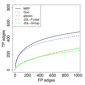
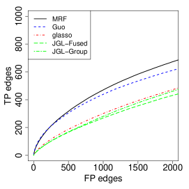
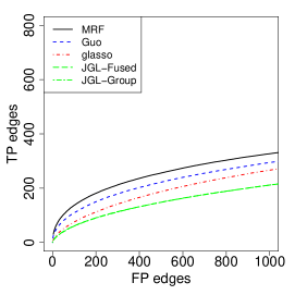
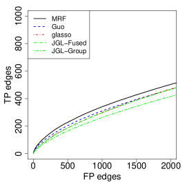
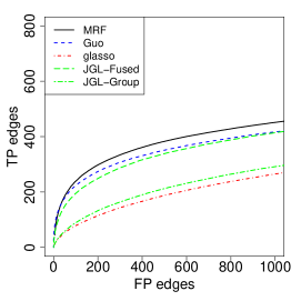
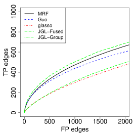
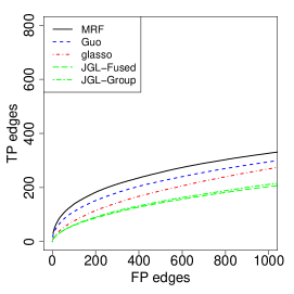
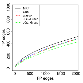
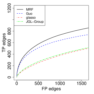
The simulation results are presented in Figure 1. Our method (MRF) was compared with Guo’s method (Guo et al., 2011), JGL (Danaher et al., 2014) and graphical lasso (glasso) (Friedman et al., 2008). In glasso, the graphs are estimated independently. In JGL, there are two options, fused lasso (JGL-Fused) and group lasso (JGL-Group). For Guo’s method, glasso and JGL, we varied the sparsity parameter to generate the curves. For our method, we varied the threshold for the marginal posterior probabilities of $\bm{\gamma}$ to generate the curves. There are two tuning parameters in JGL, $\lambda_{1}$ and $\lambda_{2}$, where $\lambda_{1}$ controls sparsity and $\lambda_{2}$ controls the strength of sharing. We performed a grid search for $\lambda_{2}$ in $\{0,0.05,...,0.5\}$ and selected the best curve. In Figure 1, our method performed slightly better than Guo’s method. When there is little shared structure among graphs, our method performed slightly better than glasso, which is possibly due to the fact that we used a different modeling framework. When the entries were different for the shared edges, JGL-Fused did not perform well. However, when the entries were the same, JGL-Fused performed much better. The fused lasso penalty encourages entries in the precision matrix to be the same and JGL-Fused gains efficiency when the assumption is satisfied.

5.2 Joint estimation of multiple graphs with temporal dependency

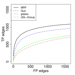
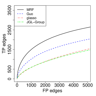
In this setting, we assumed that the graph structure evolved over time by Hidden Markov Model (HMM). We set $p=50$. At time $t=1$, we randomly selected $10\%$ among all the possible edges and set them to be edges. At time $t+1$, we removed $20\%$ of the edges at time $t$ and added back the same number of edges that were not present at time $t$. The entries in the precision matrix were set the same as that in a) in Section 5.1. We present the simulation results in Figure 2, varying $n$ and $|T|$. We compared our method with Guo’s and JGL-Group, where the graphs were treated as parallel. Our method performed better than Guo’s method and JGL-Group in all three settings, and the difference was greater when either $n$ or $|T|$ increases. We did not include JGL-Fused in the comparison as the computational time for JGL-Fused increases substantially when the number of graphs is more than a few.

(a) $n=100$, $|T|=10$

(b) $n=200$, $|T|=10$

(c) $n=100$, $|T|=30$

Figure 2: Comparisons of different models for the estimation of mutiple graphs with temporal dependency. The x-axis was truncated to be slightly larger than the total number of true positive edges. The curves represent the average of 100 independent runs.

5.3 Joint estimation of multiple graphs with both spatial and temporal dependency

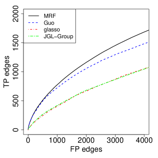
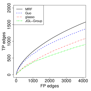
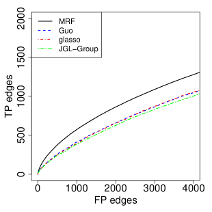
We simulated graphs in $|B|=3$ spatial loci and $|T|=10$ time periods. We set $p=50$, $n=100$, and sparsity$\sim 0.1$. We first set the graphs in different loci at the same time point to be the same. The graph structure evolved over time by HMM similarly as that in Section 5.2, and $40\%$ of the edges changed between adjacent time points. For all graphs, we then added some perturbations by removing a portion ($10\%$, $20\%$, $50\%$) of edges and adding back the same number of edges. For simplicity, we treated the spatial loci as parallel and did not simulate more complex structures. The entries in the precision matrix were set the same as that in a) in Section 5.1. The simulation results are presented in Figure 3. Our method achieved better performance than all the other methods.

(a) perturbation=0.1

(b) perturbation=0.2

(c) perturbation=0.5

Figure 3: Comparisons of different models for the estimation of mutiple graphs with temporal and spatial dependency. The x-axis was truncated to be slightly larger than the total number of true positive edges.The curves represent the average of 100 independent runs.

5.4 Computational time

We evaluated the computational speed of the Bayesian variable selection procedure in the estimation of single GGM and multiple GGMs. For single GGM, we compared our method (B-NS) with Bayesian Graphical Lasso (B-GLASSO) (Wang et al., 2012) in Figure 4a. Our algorithm took $0.5$ and $4.5$ minutes to generate 1,000 iterations for $p=100$ and $p=200$, and B-GLASSO took $1.6$ and $17.9$ minutes. We also evaluated the speed of our algorithm for the joint estimation of multiple graphs, where $n$ and $p$ were both fixed to 100. The CPU time was roughly linear as the number of graphs increased (Figure 4b). All computations presented in Figure 4 were implemented on a dual-core CPU 2.4 GHz laptop running OS X 10.9.5 using MATLAB 2014a. The computational cost of our algorithm is $O(p^{3})$. When $p=500$, for single GGM, our algorithm took $\sim 60$ minutes for 1,000 iterations. In all the previous examples, we did not implement parallel computing. The computational time may be substantially reduced when the method is implemented in parallel by multicore processors (data not shown). Even for larger $p$ ($p\geq$500), our method may still be applicable if parallel computing is implemented.

(a) Single Graph

(b) Multiple Graphs

Figure 4: CPU time for 1,000 iterations of sampling. The left plot shows the CPU time for single graph with increasing node size, we compared our method (B-NS) with Bayesian Graphical Lasso (B-GLASSO) (Wang et al., 2012). The right plot shows the CPU time with increasing number of graphs, where the node size was fixed to 100.

6 Application to the human brain gene expression dataset

Next we apply our method to the human brain gene expression microarray dataset (Kang et al., 2011). In the dataset, the expression levels of $17,568$ genes were measured in 16 brain regions across 15 time periods. The time periods are not evenly spaced over time and each time period represents a distinct stage of brain development. Because of the small sample size, we incorporated the MRF model as in equation (2) and did not consider more complex extensions: the brain regions were treated as parallel and the time periods were treated as discrete variables from $1$ to $15$. We excluded the data from time periods $1$ and $2$ in our analysis because they represent very early stage of brain development, when most of the brain regions sampled in future time periods have not differentiated. We also excluded the data where the number of replicates is less than or equal to $2$ (since a perfect line can be fitted with two data points), this step further removes $8$ groups of data: (brain region) “MD” (in time period) $4$, “S1C” $5$, “M1C” $5$, “STR” $10$, “S1C” $11$, “M1C” $11$, “STR” $11$ and “MD” $11$. The number of replicates varies across brain regions/time periods and the number is less than $10$ in general, with a few exceptions. We studied the network of $7$ genes. These $7$ genes are high confidence genes that have been implicated in their roles for Autism Spectrum Disorders (ASD): GRIN2B, DYRK1A, ANK2, TBR1, POGZ, CUL3, and SCN2A(Willsey et al., 2013). ASD is a neurodevelopment disorder that affects the brain and have an early onset in childhood. With a good understanding on the networks of the $7$ ASD genes across brain regions and time periods, we hope to gain insight into how these genes interact spatially and temporally to yield clues on their roles in autism etiology. The posterior mean and standard deviation for $\eta_{s}$ were $0.56$ and $0.51$, respectively. The posterior mean and standard deviation for $\eta_{t}$ were $0.95$ and $0.63$, respectively. The estimated model parameters suggest moderate sharing of network structure across brain regions and time.

Figure 5: The estimated graphs for all brain regions except “STR” in time period 10. Each graph corresponds to one brain region. Period 10 corresponds to early childhood ($1$ years $\leq$ age $\leq$ $6$ years), corresponding to the period of autism onset.

Figure 6: The estimated graphs for brain region “MFC” across time.

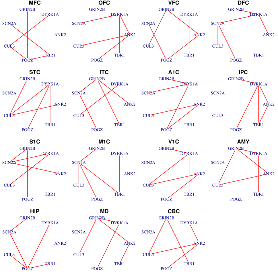
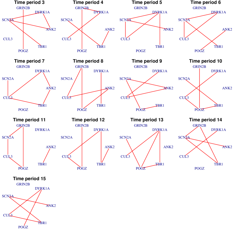
For each graph, we selected the top $5$ edges with the highest marginal posterior probabilities. Time period 10 corresponds to early childhood ($1$ years $\leq$ age $\leq$ $6$ years), which is the typical period that patients show symptoms of autism. The graphs for all brain regions except “STR” (excluded data) are shown in Figure 5. Of particular interest are the genes that are connected with TBR1, which is a transcription factor that may directly regulate the expression of numerous other genes. The edge between TBR1 and DYRK1A is mostly shared among the brain regions (7 regions). DYRK1A is a protein kinase that may play a significant role in the signaling pathway regulating cell proliferation and may be involved in brain development (Di Vona et al., 2015). It may be interesting to check whether TBR1 physically binds to DYRK1A during brain development. The graphs for region “MFC” across time are demonstrated in Figure 6. Because of the limit of space, we only show the temporal dynamics for one brain region. There are moderate sharing of edges over time. Although the edge between TBR1 and DYRK1A is not present in time period 10, it is present in time periods 5, 8, 12 and 13. Further biological experiments are required to validate whether the interaction between TBR1 and DYRK1A changes over time or it is caused by the lack of power to identify true edges due to the small sample size.

7 Conclusion

In this paper, we proposed a Bayesian neighborhood selection procedure to estimate Gaussian Graphical Models. Incorporating the Markov Random Field prior, our method was extended to jointly estimating multiple GGMs in data with complex structures. Compared with the non-Bayesian methods, there is no tuning parameter controlling the degree of structure sharing in our model. Instead, the parameters that represent similarity between graphs are learnt adaptively from the data. Simulation studies suggest that incorporating the complex data structure in the jointly modeling framework would benefit the estimation. We implemented our method by a fast and efficient algorithm that are several-fold faster than arguably the fastest algorithm for Bayesian inference of GGMs. Applying our method to the human brain gene expression data, we identified some interesting connections in the networks of autism genes during early childhood. We also demonstrated the graph selection consistency of our procedure for the estimation of single graph. The Matlab code is available at https://github.com/linzx06/Spatial-and-Temporal-GGM.

References

- (1)
- Besag (1986) Besag, J. (1986), ‘On the statistical analysis of dirty pictures’, Journal of the Royal Statistical Society. Series B (Methodological) pp. 259–302.
- Cai et al. (2011) Cai, T., Liu, W. & Luo, X. (2011), ‘A constrained l1 minimization approach to sparse precision matrix estimation’, Journal of the American Statistical Association 106(494), 594–607.
- Chun et al. (2014) Chun, H., Zhang, X. & Zhao, H. (2014), ‘Gene regulation network inference with joint sparse gaussian graphical models’, Journal of Computational and Graphical Statistics (just-accepted), 00–00.
- Danaher et al. (2014) Danaher, P., Wang, P. & Witten, D. M. (2014), ‘The joint graphical lasso for inverse covariance estimation across multiple classes’, Journal of the Royal Statistical Society: Series B (Statistical Methodology) 76(2), 373–397.
- Di Vona et al. (2015) Di Vona, C., Bezdan, D., Islam, A. B., Salichs, E., López-Bigas, N., Ossowski, S. & de la Luna, S. (2015), ‘Chromatin-wide profiling of dyrk1a reveals a role as a gene-specific rna polymerase ii ctd kinase’, Molecular cell 57(3), 506–520.
- Dobra et al. (2011) Dobra, A., Lenkoski, A. & Rodriguez, A. (2011), ‘Bayesian inference for general gaussian graphical models with application to multivariate lattice data’, Journal of the American Statistical Association 106(496).
- Friedman et al. (2008) Friedman, J., Hastie, T. & Tibshirani, R. (2008), ‘Sparse inverse covariance estimation with the graphical lasso’, Biostatistics 9(3), 432–441.
- George & McCulloch (1993) George, E. I. & McCulloch, R. E. (1993), ‘Variable selection via gibbs sampling’, Journal of the American Statistical Association 88(423), 881–889.
- George & McCulloch (1997) George, E. I. & McCulloch, R. E. (1997), ‘Approaches for bayesian variable selection’, Statistica sinica 7(2), 339–373.
- Guo et al. (2011) Guo, J., Levina, E., Michailidis, G. & Zhu, J. (2011), ‘Joint estimation of multiple graphical models’, Biometrika p. asq060.
- Hastie et al. (2009) Hastie, T., Tibshirani, R., Friedman, J., Hastie, T., Friedman, J. & Tibshirani, R. (2009), The elements of statistical learning, Vol. 2, Springer.
- Kanehisa & Goto (2000) Kanehisa, M. & Goto, S. (2000), ‘Kegg: kyoto encyclopedia of genes and genomes’, Nucleic acids research 28(1), 27–30.
- Kang et al. (2011) Kang, H. J., Kawasawa, Y. I., Cheng, F., Zhu, Y., Xu, X., Li, M., Sousa, A. M., Pletikos, M., Meyer, K. A., Sedmak, G. et al. (2011), ‘Spatio-temporal transcriptome of the human brain’, Nature 478(7370), 483–489.
- Li & Zhang (2010) Li, F. & Zhang, N. R. (2010), ‘Bayesian variable selection in structured high-dimensional covariate spaces with applications in genomics’, Journal of the American Statistical Association 105(491).
- Lin et al. (2015) Lin, Z., Sanders, S. J., Li, M., Sestan, N., Zhao, H. et al. (2015), ‘A markov random field-based approach to characterizing human brain development using spatial–temporal transcriptome data’, The Annals of Applied Statistics 9(1), 429–451.
- Meinshausen & Bühlmann (2006) Meinshausen, N. & Bühlmann, P. (2006), ‘High-dimensional graphs and variable selection with the lasso’, The Annals of Statistics pp. 1436–1462.
- Narisetty et al. (2014) Narisetty, N. N., He, X. et al. (2014), ‘Bayesian variable selection with shrinking and diffusing priors’, The Annals of Statistics 42(2), 789–817.
- Orchard et al. (2013) Orchard, P., Agakov, F. & Storkey, A. (2013), ‘Bayesian inference in sparse gaussian graphical models’, arXiv preprint arXiv:1309.7311 .
- Peterson et al. (2014) Peterson, C., Stingo, F. & Vannucci, M. (2014), ‘Bayesian inference of multiple gaussian graphical models’, Journal of the American Statistical Association (just-accepted), 00–00.
- Rual et al. (2005) Rual, J.-F., Venkatesan, K., Hao, T., Hirozane-Kishikawa, T., Dricot, A., Li, N., Berriz, G. F., Gibbons, F. D., Dreze, M., Ayivi-Guedehoussou, N. et al. (2005), ‘Towards a proteome-scale map of the human protein–protein interaction network’, Nature 437(7062), 1173–1178.
- Shen-Orr et al. (2002) Shen-Orr, S. S., Milo, R., Mangan, S. & Alon, U. (2002), ‘Network motifs in the transcriptional regulation network of escherichia coli’, Nature genetics 31(1), 64–68.
- Wang et al. (2012) Wang, H. et al. (2012), ‘Bayesian graphical lasso models and efficient posterior computation’, Bayesian Analysis 7(4), 867–886.
- Willsey et al. (2013) Willsey, A. J., Sanders, S. J., Li, M., Dong, S., Tebbenkamp, A. T., Muhle, R. A., Reilly, S. K., Lin, L., Fertuzinhos, S., Miller, J. A. et al. (2013), ‘Coexpression networks implicate human midfetal deep cortical projection neurons in the pathogenesis of autism’, Cell 155(5), 997–1007.
- Yuan & Lin (2007) Yuan, M. & Lin, Y. (2007), ‘Model selection and estimation in the gaussian graphical model’, Biometrika 94(1), 19–35.
- Zhang & Horvath (2005) Zhang, B. & Horvath, S. (2005), ‘A general framework for weighted gene co-expression network analysis’, Statistical applications in genetics and molecular biology 4(1).
- Zhang & Huang (2008) Zhang, C.-H. & Huang, J. (2008), ‘The sparsity and bias of the lasso selection in high-dimensional linear regression’, The Annals of Statistics pp. 1567–1594.