Multiscale model reduction for shale gas transport in fractured media

Abstract

In this paper, we develop a multiscale model reduction technique that describes shale gas transport in fractured media. Due to the pore-scale heterogeneities and processes, we use upscaled models to describe the matrix. We follow our previous work [1], where we derived an upscaled model in the form of generalized nonlinear diffusion model to describe the effects of kerogen. To model the interaction between the matrix and the fractures, we use Generalized Multiscale Finite Element Method [13, 17]. In this approach, the matrix and the fracture interaction is modeled via local multiscale basis functions. In [17], we developed the GMsFEM and applied for linear flows with horizontal or vertical fracture orientations on a Cartesian fine grid. In this paper, we consider arbitrary fracture orientations and use triangular fine grid and developed GMsFEM for nonlinear flows. Moreover, we develop online basis function strategies to adaptively improve the convergence. The number of multiscale basis functions in each coarse region represents the degrees of freedom needed to achieve a certain error threshold. Our approach is adaptive in a sense that the multiscale basis functions can be added in the regions of interest. Numerical results for two-dimensional problem are presented to demonstrate the efficiency of proposed approach.

1 Introduction

Shale gas transport is an active area of research due to a growing interest in producing natural gas from source rocks. The shale systems have added complexities due to the presence of organic matter, known as kerogen. The kerogen brings in new fluid storage and transport qualities to the shale. A number of authors, e.g., Loucks et al. (2009), Sondergeld et al. (2010), and Ambrose et al. (2012), [26, 31, 3], have previously discussed the physical properties of the kerogen using scanning electron microscopy (SEM) and showed the co-existence of nanoporous kerogen and microporous conventional inorganic rock materials.

Gas transport in the kerogen typically develops at low Reynolds number and relatively high Knudsen number values. Under these conditions, it is expected that the transport is not driven by laminar (Darcy) flow dominantly but instead by the pore diffusion and other molecular transport mechanisms such as Knudsen diffusion and the adsorbed phase (or surface) diffusion. The latter introduces nonlinear processes at the pore scale that occur in heterogeneous pore geometry. Some types of upscaled models are needed to represent these complex processes for reservoir simulations.

In large-scale simulations, the complex pore-scale transport needs to be coupled to the transport in fractures. This brings an additional difficulty in multiscale simulations. In particular, the multiscale simulations of the processes describing the interaction between the fracture and the matrix require reduced-order model approaches that work for problems without scale separation and high contrast. The objective of this paper is to discuss the development of such approaches for describing the fracture and the matrix interaction by taking the upscaled matrix model following our previous work [1].

In our previous work [1], we proposed a set of macroscopic models that take into account the nanoporous nature and nonlinear processes of the shale matrix. Our derivation uses multiple scale asymptotic analysis applied to mass balance equations, equation of state (for free gas) and isotherm of adsorption. The fine-scale microscopic description is largely based on the model formulated by Akkutlu and Fathi (2012), [2]. The macroscopic parameters that appear in the equations require solutions of cell problem defined in representative volume elements (RVEs). These RVE problems take into account fine-scale variations and average their effects on macro scale.

The multiscale approaches proposed in [1] are limited to representing the features that have scale separation. To represent the fracture network and the interaction between the fracture network and the matrix, we present a multiscale approach following the framework of Generalized Multiscale Finite Element Method (GMsFEM), [13]. The main idea of GMsFEM is to use multiscale basis functions to extract an essential information in each coarse grid (computational grid) and develop a reduced-order model. In [17], we have developed the GMsFEM and applied for linear flows with horizontal or vertical fracture orientations on a Cartesian fine grid. In this paper, our contributions are: (1) the use of arbitrary fracture orientations and use triangular fine grids; (2) the development of GMsFEM for nonlinear flows; and (3) the development of online basis function strategies to adaptively improve the convergence.

To represent the fractures on the fine grid, we use Discrete Fracture Model (DFM) [35]. The fine grid is constructed to resolve the fractures. For the coarse grid, we choose a rectangular grid. The GMsFEM framework uses these fine-scale models in computing the snapshot space and the offline space. The nonlinear models are handled with GMsFEM by locally updating multiscale basis functions.

The study of flows in fractured media has a long history. Some modeling techniques on the fine grid include the Discrete Fracture Model (DFM), Embedded Fracture Model (EFM) [27, 25, 23], the single-permeability model, the multiple-permeability models ([33, 4, 28, 23, 20, 34, 30, 10]), and hierarchical fracture models [23]. Though these approaches are designed for fine-scale simulations, a number of these approaches represent the fractures at a macroscopic level. For example, multiple-permeability models represent the network of connected fractures macroscopically by introducing several permeabilities in each block. The EFM ([27, 25, 23]) models the interaction of fractures with the fine-grid blocks separately for each block. The main idea of hierarchical fracture modeling presented in [23] is to homogenize small-length fractures (with the length smaller than the coarse block), while to represent the large-length fractures. Some of these approaches can be generalized by incorporating the interaction of fractures and permeability heterogeneities locally, which can lead to efficient upscaling techniques, [11, 19].

In recent papers [21], several multiscale approaches are proposed for representing the fracture effects. These approaches share common concepts with the methods that we discuss here in a sense that they add new degrees of freedom to represent the fractures on a coarse grid. The main difference is that our approaches use local spectral problems accompanied by adaptivity to detect the regions, where to add new basis functions. In this regard, the procedure of finding multiscale basis functions and the enrichment procedure is different from existing techniques.

The proposed method constructs multiscale basis functions by appropriately selecting local snapshot space and the local spectral problems for the underlying nonlinear problem. The local spectral problems allow us to adaptively enrich in the regions with larger errors. In the paper, we discuss adaptivity issues and how to add multiscale basis functions in some selected regions. To reduce the computational cost associated with constructing the snapshot space, we follow [5] and use randomized boundary conditions. One of other novel components of the paper is the use of online basis functions (see [8] for online basis functions for steady state problems) for the time-dependent nonlinear problems. The online basis functions are constructed during the simulation using the residual and they can reduce the error significantly. These basis functions are used if the offline basis functions can not reduce the error below a desired threshold.

We present numerical results for some representative examples. In these examples, we use nonlinear matrix and fracture models. Our numerical results show that the coarse-scale models with a fewer degrees of freedom can be used to get an accurate approximation of the fine-scale solution. In particular, only 10 % degrees of the freedom are needed to obtain an accurate representation of the fine-scale solution. We also add a geomechanical contribution to the permeability term, where the permeability depends on the pressure. Furthermore, we demonstrate the use of online basis functions and how they can reduce the error.

The paper is organized as follows. In the next section, we present a model problem. In Section 3, we discuss the fine-scale model. Section 4 is devoted to the development of GMsFEM, in particular, the offline spaces. In this section, we present numerical results for offline basis functions. In Section 5, we discuss randomized snapshot spaces and show that their use can give similar accuracy while for less computational cost. In Section 6, we develop online basis functions and present numerical results.

2 Model Problem

In this paper, we will study nonlinear gas transport in fractured media motivated by several applications including shale gas. We are interested in the shale gas transport described in [2]. Similar equations arise in other models, where one considers a free gas in the tight reservoirs. We will consider general equations

$$a_{m}(c){\partial c\over\partial t}=\text{div}(b_{m}(c,x)\nabla c),$$ (1)

where $c$ is the amount of free gas and $a(c)$ and $b(c)$ contain terms related to storage and adsorption coefficients. In [2], the authors consider the nonlinear terms have the forms

$$a_{m}(c)=\phi+(1-\phi)\gamma\frac{\partial F}{\partial c},\quad b_{m}(c,x)=\phi D+(1-\phi)\gamma D_{s}\frac{\partial F}{\partial c}+\phi\frac{\kappa}{\mu}RTc,$$

where $\gamma$ is a parameter, which is unity in kerogen and is equal to $V_{grain,k}/V_{grain}$ in the inorganic material ($V_{grain,k}$ is grain volume and $V_{grain}$ is kerogen grain volume). Diffusivity $D$ and porosity $\phi$ are defined for the free fluid in the inorganic matrix and in the kerogen as follows

$$D=\begin{cases}D_{k}&\text{ in kerogen}\\ D_{i}&\text{ in inorganic matrix}\end{cases},\quad\phi=\begin{cases}\phi_{k}&\text{ in kerogen}\\ \phi_{i}&\text{ in inorganic matrix}\end{cases}.$$

For the free gas we have ideal gas assumption. The Darcy law of free gas flow in inorganic matrix is used with permeability $\kappa$ and gas viscosity $\mu$. For the sorbed gas we can use Langmuir or Henry‘s isotherms $F=F(c)$. In [24, 35], the authors discuss a general framework, where the equations also include nonlinear diffusivity due to adsorbed gas in a shale formation. In [22], the nonlinear terms appear due to barotropic effects.

The nonlinear flows also contain components that are due to diffusion in the fractures. One needs additional equations for modeling fractures. The fractures have high conductivity. We will use a general equation of the form

$$a_{f}(c){\partial c\over\partial t}=\text{div}(b_{f}(c,x)\nabla c)$$ (2)

to describe the flow within fractures. In [2], the authors use

$$a_{f}(c)=\phi_{f},\quad b_{f}(c,x)=\frac{\kappa_{f}}{\mu}RTc,$$

where $\phi_{f}$ and $\kappa_{f}$ are the fracture porosity and permeability. These problems are solved on a fine grid using DFM as will be described in Section 3.

In many shale gas examples, the matrix heterogeneities can be upscaled and the resulting upscaled equation has the form (1). However, the interaction between matrix and fractures require some type of multiscale modeling approach, where the effects of the fractures need to be captured more accurately. Approaches, such as multicontinuum [24] are often used, but these approaches use idealized assumptions on fracture distributions. In this paper, we will use multiscale basis functions to represent fracture effects. In our previous work [17], we have considered similar approaches for single-phase flow when fractures (which could be horizontal or vertical) are aligned with Cartesian grid. In this paper, we consider arbitrary fracture distribution in the context of nonlinear flow equations.

The overall model equations will be solved on a coarse grid. Next, we introduce the concepts of fine and coarse grids. Let $\mathcal{T}^{H}$ be a usual conforming partition of the computational domain $\Omega$ into finite elements (triangles, quadrilaterals, tetrahedra, etc.). We refer to this partition as the coarse grid and assume that each coarse element is partitioned into a connected union of fine grid blocks. The fine grid partition will be denoted by $\mathcal{T}^{h}$, and is by definition a refinement of the coarse grid $\mathcal{T}^{H}$. We use $\{x_{i}\}_{i=1}^{N}$ (where $N$ denotes the number of coarse nodes) to denote the vertices of the coarse mesh $\mathcal{T}^{H}$ and define the neighborhood of the node $x_{i}$ by

$$\omega_{i}=\bigcup\{K_{j}\in\mathcal{T}^{H};~{}~{}~{}x_{i}\in\overline{K}_{j}\}.$$ (3)

Figure 1: Illustration of a coarse neighborhood and coarse element

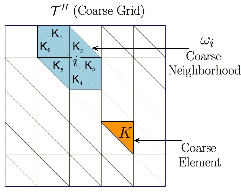
See Figure 1 for an illustration of neighborhoods and elements subordinated to the coarse discretization. We emphasize the use of $\omega_{i}$ to denote a coarse neighborhood, and $K$ to denote a coarse element throughout the paper.

3 Fine-scale discretization

To discretize the system on fine grid, we will use finite element method and use DFM for fractures. To solve Problem (1) using finite element method (FEM), we need a fine grid discretization to capture the fractures. These computations can be expensive. Here, we apply the discrete fracture network (DFM) model for modeling flows in fractures [29].

In the discrete-fracture model, the aperture of the fracture appears as a factor in front of the one dimensional integral for the consistency of the integral form. This is the main idea of the discrete-fracture model, which can be applied in any complex configuration for fractured porous media.

To demonstrate it, we consider the two-dimensional problem of Equation (2). We simplify the fractures as the lines with small aperture. Thus, one-dimensional element is needed to describe fractures in the discrete-fracture model. The system of equations (1) will be discretized in a two-dimensional form for the matrix and in one-dimensional form for the fractures. The whole domain $\Omega$ can be represented by

$$\Omega=\Omega_{m}\oplus_{i}\,d_{i}\Omega_{f,i},$$ (4)

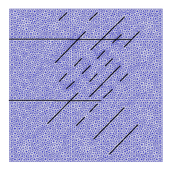
where $m$ and $f$ represent the matrix and the fracture of the permeability field $\kappa$, respectively. Here, $d_{i}$ is the aperture of the $i$ th fracture and $i$ is the index of the fractures. Note that $\Omega_{m}$ is a two-dimensional domain and $\Omega_{f,i}$ is a one-dimensional domain (Figure 2). Then Equations (1) and (2) and can be written as follows (for any test function $v$):

$$\begin{split}m(\frac{\partial c}{\partial t},v)+a(c,v)&=\int_{\Omega_{m}}a_{m}(c){\partial c\over\partial t}v\,dx+d_{i}\sum\limits_{i}\int_{\Omega_{f,i}}a_{f}(c){\partial c\over\partial t}v\,dx+\\ &+\int_{\Omega_{m}}b_{m}(c,x)\nabla c\cdot\nabla v\,dx+d_{i}\sum\limits_{i}\int_{\Omega_{f,i}}b_{m}(c,x)\nabla c\cdot\nabla v\,dx=0.\end{split}$$ (5)

Figure 2: Fine grid with fractures

To solve (5), we will first linearize the system. We will use the following linearization

$$\begin{split}m({c^{n+1}-c^{n}\over\tau},v)+a(c^{n+1},v)&=\int_{\Omega_{m}}a_{m}(c^{n}){c^{n+1}-c^{n}\over\tau}v\,dx+d_{i}\sum\limits_{i}\int_{\Omega_{f,i}}a_{f}(c^{n}){c^{n+1}-c^{n}\over\tau}v\,dx+\\ &+\int_{\Omega_{m}}b_{m}(c^{n},x)\nabla c^{n+1}\cdot\nabla v\,dx+d_{i}\sum\limits_{i}\int_{\Omega_{f,i}}b_{f}(c^{n},x)\nabla c^{n+1}\cdot\nabla v\,dx=0.\end{split}$$ (6)

The standard fully-implicit finite difference scheme is used for the approximation with time step size $\tau$ and superscripts $n$, $n+1$ denote previous and current time levels. This is a first-order in time and unconditionally stable linearization.

For standard Galerkin finite element method, we write the solution as $c=\sum_{i=1}^{N_{f}}c_{i}\phi_{i}$, where $\phi_{i}$ are the standard linear element basis functions defined on $\mathcal{T}^{h}$ and $N_{f}$ denotes the number of the nodes on the fine grid. The equation (6) can be presented in matrix form:

$$M^{n}\frac{c^{n+1}-c^{n}}{\tau}+A^{n}c^{n+1}=0,$$ (7)

where $M$ is the mass matrix given by

$$M^{n}=[m_{ij}]=\int_{\Omega_{m}}a_{m}(c^{n})\phi_{i}\phi_{j}\,dx+d_{i}\sum\limits_{i}\int_{\Omega_{f,i}}a_{f}(c^{n})\phi_{i}\phi_{j}\,dx,$$

and $A$ is the stiffness matrix given by

$$A^{n}=[a_{ij}]=\int_{\Omega_{m}}b_{m}(c^{n},x)\nabla\phi_{i}\cdot\nabla\phi_{j}\,dx+d_{i}\sum\limits_{i}\int_{\Omega_{f,i}}b_{f}(c^{n},x)\nabla\phi_{i}\cdot\nabla\phi_{j}\,dx.$$

Hence at each time step we have the following linear problem

$$Q^{n}c^{n+1}=M^{n}c^{n},$$ (8)

where $Q^{n}=\left(M^{n}+\tau A^{n}\right)$. This fine scale discretization yields large matrices of size $N_{f}\times N_{f}$.

4 Coarse-grid discretization using GMsFEM. Offline spaces.

We use multiscale basis functions to represent the solution space. We will consider the continuous Galerkin (CG) formulation and signify $\omega_{i}$ as the support of basis functions. We denote the basis functions by $\psi_{k}^{\omega_{i}}$, which is supported in $\omega_{i}$, and the index $k$ represents the numbering of these basis functions. In turn, the CG solution will be sought as

$$c_{\text{ms}}(x,t)=\sum_{i,k}c_{k}^{i}(t)\psi_{k}^{\omega_{i}}(x).$$

Once the basis functions are identified, the CG global coupling is given through the variational form

$$m(\frac{\partial c}{\partial t},v)+a(c_{\text{ms}},v)=0,\quad\text{for all}\,\,v\in V_{\text{off}},$$ (9)

where $V_{\text{off}}$ is used to denote the space spanned by those basis functions and

$$m(c,v)=\int_{\Omega_{m}}a_{m}c\,v\,dx+d_{i}\sum\limits_{i}\int_{\Omega_{f,i}}a_{f}c\,v\,dx,$$

$$a(c,v)=\int_{\Omega_{m}}b_{m}\nabla c\cdot\nabla v\,dx+d_{i}\sum\limits_{i}\int_{\Omega_{f,i}}b_{f}\nabla c\cdot\nabla v\,dx.$$

Let $V$ be the conforming finite element space with respect to the fine-scale partition $\mathcal{T}^{h}$. We assume $c\in V$ is the fine-scale solution satisfying

$$m(\frac{\partial c}{\partial t},v)+a(c,v)=0,\quad v\in V.$$ (10)

Next, we describe GMsFEM. GMsFEM consists of offline and online stage. In the offline stage we construct multiscale basis functions and after that in the online stage, we solve our problem for any input parameters, such as right hand sides or boundary conditions.

Offline computations:

• Step 1. Coarse grid generation.

• Step 2. Construction of the snapshot space that will be used to compute an offline space.

• Step 3. Construction of a “small” dimensional offline space by performing dimension reduction in the space of local snapshots.

Given the computational domain, a coarse grid can be constructed and local problems are solved on coarse neighborhoods to obtain the snapshot spaces. Then, smaller dimensional offline spaces are obtained from the snapshot spaces by dimension reduction via some spectral problems [13, 12, 16, 14, 5]. After that we can solve our problem in the constructed offline space. Moreover, we will construct online basis functions that are problem dependent and are computed locally based on some local residuals [9, 8].

We now present the construction of the offline basis functions and the corresponding spectral problems for obtaining a space reduction. In the offline computation, we first construct a snapshot space $V_{\text{snap}}^{\omega}$. The snapshot space can be the space of all fine-scale basis functions or the solutions of some local problems with various choices of boundary conditions. For example, we can use the following $\kappa$-harmonic extensions to form a snapshot space. For each fine-grid function, $\delta_{j}^{h}(x)$, which is defined by $\delta_{j}^{h}(x)=\delta_{j,k},\,\forall j,k\in\textsl{J}_{h}(\omega_{i})$, where $\textsl{J}_{h}(\omega_{i})$ denotes the fine-grid boundary node on $\partial\omega_{i}$. For simplicity, we omit the index $i$. Given a fine-scale piecewise linear function defined on $\partial\omega$ (here $\omega$ is a generic coarse element), we define $\psi_{j}^{\omega,\text{snap}}$ by following variational problem

$$a(\psi_{j}^{\omega,\text{snap}},v)=\int_{\omega_{m}}b_{m}\nabla\psi_{j}^{\omega,\text{snap}}\cdot\nabla v\,dx+d_{j}\sum\limits_{j}\int_{\omega_{f,j}}b_{f}\nabla\psi_{j}^{\omega,\text{snap}}\cdot\nabla v\,dx=0\quad\text{in }\,\omega,$$ (11)

and $\psi_{j}^{\omega,\text{snap}}=\delta_{j}^{h}(x)$ on $\partial\omega$, $\omega=\omega_{m}\oplus_{j}\,d_{j}\omega_{f,j}$.

For brevity of notation, we now omit the superscript $\omega$, yet it is assumed throughout this section that the offline space computations are localized to respective coarse subdomains. Let $l_{i}$ be the number of functions in the snapshot space in the region $\omega$, and

$$V_{\text{snap}}=\text{span}\{\psi_{j}^{\text{snap}}:~{}~{}~{}1\leq j\leq l_{i}\},$$

for each coarse subdomain $\omega$.

Denote

$$R_{\text{snap}}=\left[\psi_{1}^{\text{snap}},\ldots,\psi_{l_{i}}^{\text{snap}}\right].$$

In order to construct the offline space $V_{\text{off}}^{\omega}$, we perform a dimension reduction of the snapshot space using an auxiliary spectral decomposition. The analysis in [15] motivates the following eigenvalue problem in the space of snapshots:

$$A^{\text{off}}\Psi_{k}^{\text{off}}=\lambda_{k}^{\text{off}}S^{\text{off}}\Psi_{k}^{\text{off}},$$ (12)

where

$$A^{\text{off}}=[a_{mn}^{\text{off}}]=\int_{\omega_{m}}b_{m}\nabla\psi_{m}^{\text{snap}}\cdot\nabla\psi_{n}^{\text{snap}}\,dx+d_{j}\sum\limits_{j}\int_{\omega_{f,j}}b_{f}\nabla\psi_{m}^{\text{snap}}\cdot\nabla\psi_{n}^{\text{snap}}\,dx=R_{\text{snap}}^{T}AR_{\text{snap}},$$

$$S^{\text{off}}=[s_{mn}^{\text{off}}]=\int_{\omega_{m}}b_{m}\psi_{m}^{\text{snap}}\psi_{n}^{\text{snap}}\,dx+d_{j}\sum\limits_{j}\int_{\omega_{f,j}}b_{f}\psi_{m}^{\text{snap}}\psi_{n}^{\text{snap}}\,dx=R_{\text{snap}}^{T}SR_{\text{snap}},$$

where $A$ and $S$ denote analogous fine scale matrices as defined by

$$A_{ij}=\int_{D_{m}}b_{m}(c^{n},x)\nabla\phi_{i}\cdot\nabla\phi_{j}\,dx+d_{i}\sum\limits_{i}\int_{D_{f,i}}b_{f}(c^{n},x)\nabla\phi_{i}\cdot\nabla\phi_{j}\,dx,$$

$$S_{ij}=\int_{D_{m}}b_{m}(c^{n})\phi_{i}\phi_{j}\,dx+d_{i}\sum\limits_{i}\int_{D_{f,i}}b_{f}(c^{n})\phi_{i}\phi_{j}\,dx,$$

where $\phi_{i}$ is the fine-scale basis function. To generate the offline space, we then choose the smallest $M^{\omega}_{\text{off}}$ eigenvalues from Eq. (12) and form the corresponding eigenvectors in the space of snapshots by setting $\psi_{k}^{\text{off}}=\sum_{j=1}^{l_{i}}\Psi_{kj}^{\text{off}}\psi_{j}^{\text{snap}}$ (for $k=1,\ldots,M^{\omega}_{\text{off}}$), where $\Psi_{kj}^{\text{off}}$ are the coordinates of the vector $\Psi_{k}^{\text{off}}$.

Next, we create an appropriate solution space and variational formulation that for a continuous Galerkin approximation. We begin with an initial coarse space $V^{\text{init}}_{0}=\text{span}\{\chi_{i}\}_{i=1}^{N}$. Recall that $N$ denotes the number of coarse neighborhoods. Here, $\chi_{i}$ are the standard multiscale partition of unity functions defined by

$$a(\chi_{i},v)=\int_{\omega_{m}}b_{m}\nabla\chi_{i}\cdot\nabla v\,dx+d_{j}\sum\limits_{j}\int_{\omega_{f,j}}b_{f}\nabla\chi_{i}\cdot\nabla v\,dx=0\quad K\in\omega$$ (13)

$$\chi_{i}=g_{i}\quad\text{on}\,\,\,\partial K,$$

for all $K\in\omega$, where $g_{i}$ is a continuous function on $\partial K$ and is linear on each edge of $\partial K$.

We then multiply the partition of unity functions by the eigenfunctions in the offline space $V_{\text{off}}^{\omega_{i}}$ to construct the resulting basis functions

$$\psi_{i,k}=\chi_{i}\psi_{k}^{\omega_{i},\text{off}}\quad\text{for}\,\,\,1\leq i\leq N\,\,\,\text{and}\,\,\,1\leq k\leq M_{\text{off}}^{\omega_{i}},$$ (14)

where $M_{\text{off}}^{\omega_{i}}$ denotes the number of offline eigenvectors that are chosen for each coarse node $i$. We note that the construction in Eq. (14) yields continuous basis functions due to the multiplication of offline eigenvectors with the initial (continuous) partition of unity. Next, we define the continuous Galerkin spectral multiscale space as

$$V_{\text{off}}=\text{span}\{\psi_{i,k}:\,\,1\leq i\leq N\,\,\,\text{and}\,\,\,1\leq k\leq M_{\text{off}}^{\omega_{i}}\}.$$ (15)

Using a single index notation, we may write $V_{\text{off}}=\text{span}\{\psi_{i}\}_{i=1}^{N_{c}}$, where $N_{c}=\sum_{i=1}^{N}M_{\text{off}}^{\omega_{i}}$ denotes the total number of basis functions in the space $V_{\text{off}}$. We also construct an operator matrix

$$R_{0}^{T}=\left[\psi_{1},\ldots,\psi_{N_{c}}\right],$$

where $\psi_{i}$ are used to denote the nodal values of each basis function defined on the fine grid.

We seek $c_{\text{ms}}(x)=\sum_{i}c_{i}\psi_{i}(x)\in V_{\text{off}}$ such that

$$m(\frac{\partial c_{\text{ms}}}{\partial t},v)+a(c_{\text{ms}},v)=0\quad\text{for all}\,\,\,v\in V_{\text{off}}.$$ (16)

We note that variational form in (16) yields the following linear algebraic system

$$Q^{n}_{0}c_{0}^{n+1}=M^{n}_{0}c_{0}^{n},$$ (17)

where $c_{0}$ denotes the nodal values of the discrete CG solution, and $Q^{n}_{0}=R_{0}Q^{n}R_{0}^{T}$ and $M_{0}^{n}=R_{0}M^{n}$. We also note that the operator matrix may be analogously used in order to project coarse scale solutions onto the fine grid $c^{n+1}=R_{0}^{T}c_{0}^{n+1}$. In our simulations presented next, we do not update basis functions. We discuss basis function update in Section 6.

4.1 Numerical result

We present numerical results for the coarse-scale solution using offline basis functions. The basis functions of the offline space are constructed following the procedure described above. Note that, the basis functions are constructed only once at initial time and used for generating the stiffness matrix and the right hand side.

We consider the solution of problem with constant and nonlinear matrix-fracture coefficients in (6). As constant coefficients (see previous section) representing matrix and fracture properties, we use following

$$a_{m}=0.8,\quad b_{m}=1.3\cdot 10^{-7}\quad\text{and}\quad a_{f}=0.001,\quad b_{f}=1.0.$$

For nonlinear matrix-fracture coefficients, we use

$$a_{{m}}(c)=\phi+(1-\phi)\frac{\partial F}{\partial c},\quad b_{m}(c,x)=\phi D+(1-\phi)D_{s}\frac{\partial F}{\partial c}+\phi\frac{\kappa}{\mu}RTc,$$ (18)

and

$$a_{f}(c)=\phi_{f},\quad b_{f}(c,x)=\frac{\kappa_{f}}{\mu}RTc,$$ (19)

where $D_{k}=10^{-7}[m^{2}/s]$, $D_{i}=10^{-8}[m^{2}/s]$, $\phi=0.04$, $T=413[K]$, $\mu=2\cdot 10^{-5}[kg/(m\,s)]$ and for fractures $k_{f}=10^{-12}[m^{2}]$, $\phi_{f}=0.001$.

As for permeability $\kappa$ in (18), we use constant $\kappa=\kappa_{0}$ and stress-dependent model $\kappa=\kappa_{m}$ (see [18, 32]) with

$$\kappa_{m}=\kappa_{0}\left(1-\left(\frac{p_{c}-\alpha p}{p_{1}}\right)^{\mathcal{M}}\right)^{3},$$

where $\kappa_{0}=10^{-18}[m^{2}]$, $p=RTc$, $p_{c}=10^{9}[Pa]$, $p_{1}=1.8\cdot 10^{9}[Pa]$, $\alpha=0.5$ and $\mathcal{M}=0.5$. For the sorbed gas, we use Langmuir model

$$F(c)=c_{\mu s}\frac{s}{(1+sc)^{2}},$$

where $s=0.26\cdot 10^{-3}$ and $c_{\mu s}=0.25\cdot 10^{-5}[mol/m^{3}]$.

Figure 3: Coarse and fine grids. Coarse grid contains 50 cells, 85 facets and 36 vertices. Fine grid contains 7580 cells, 11470 facets and 3891 vertices.

Figure 4: Coarse and fine grids. Coarse grid contains 200 cells, 320 facets and 121 vertices. Fine grid contains 13036 cells, 19694 facets and 6659 vertices.

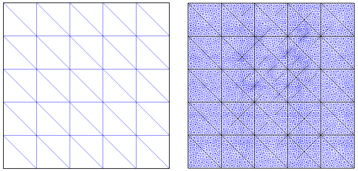
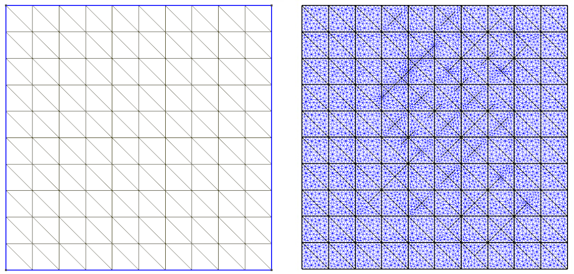
The equation is solved with Dirichlet boundary condition $c(x,t)=5000$ on the left boundary and Neumann boundary conditions $\frac{\partial c(x,t)}{\partial n}=0$ on other boundaries. The domain $\Omega$ has a length of 60 meters in both directions. We calculate concentration for $t_{max}=5$ years with the time step $\tau=10$ days. As for initial condition, we use $c(x,t=0)=10000[mol/m^{3}]$. For the numerical solution, we construct structured two coarse grids with 36 nodes (Figure 3) and with 121 nodes (Figure 4). As for fine grids, we use unstructured grids, which resolves the existing fractures.

Figure 5: Solution with constant matrix-fracture coefficients on coarse (top) and on fine (bottom) grids for t=1, 3 and 5 year (from top to bottom)

Figure 6: Coarse-scale (top) and fine-scale (bottom) solutions for t=5 year for the case of nonlinear permeability with $\kappa=\kappa_{0}$

Figure 7: Coarse-scale (top) and fine-scale (bottom) solutions for t=5 year for the case of nonlinear coefficients with $\kappa=\kappa_{m}$

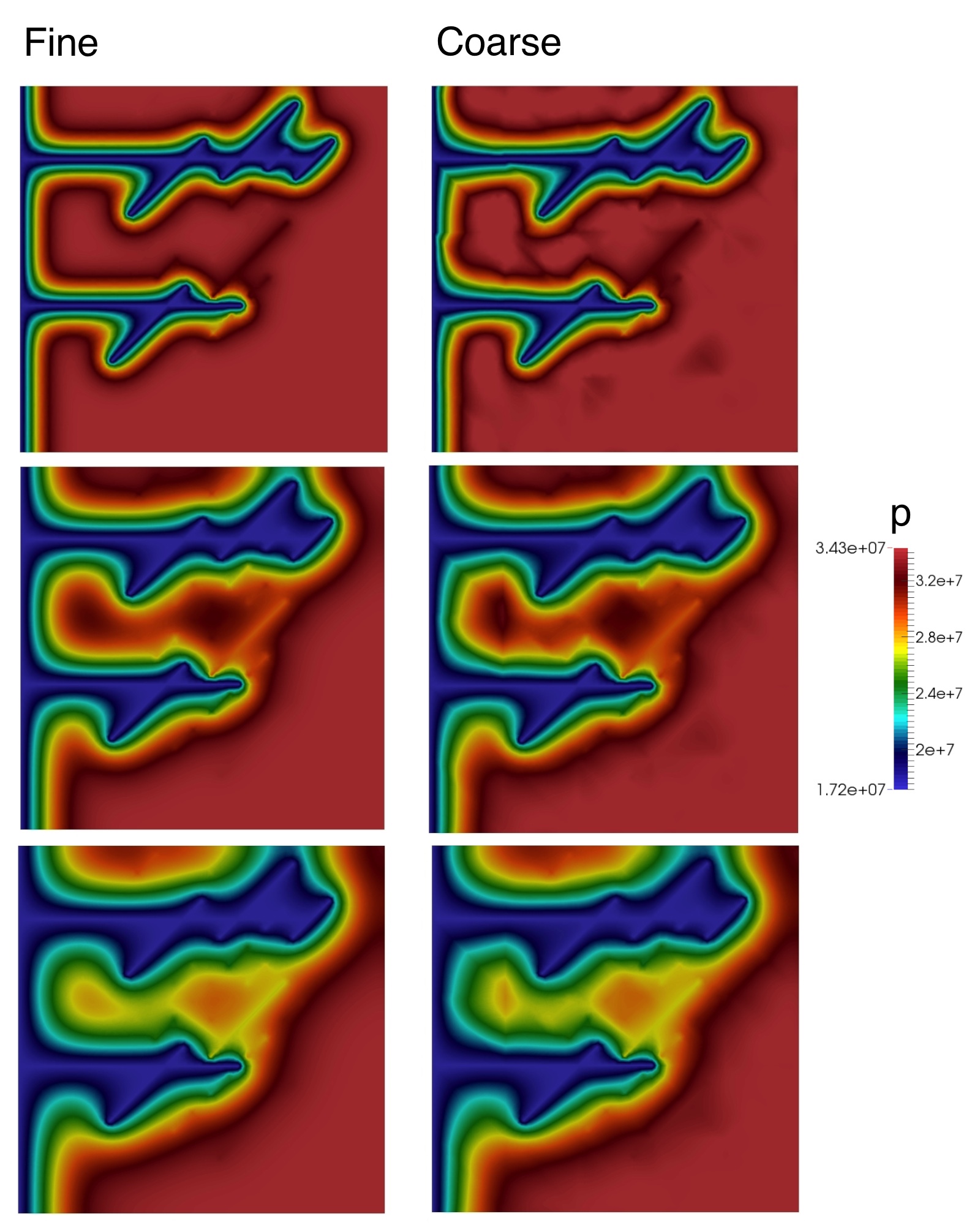
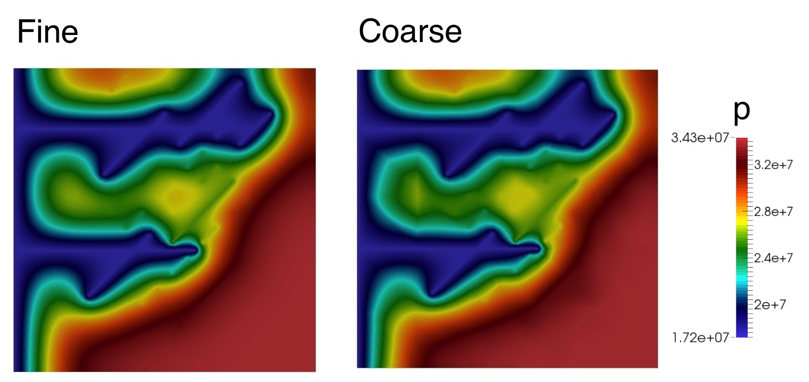
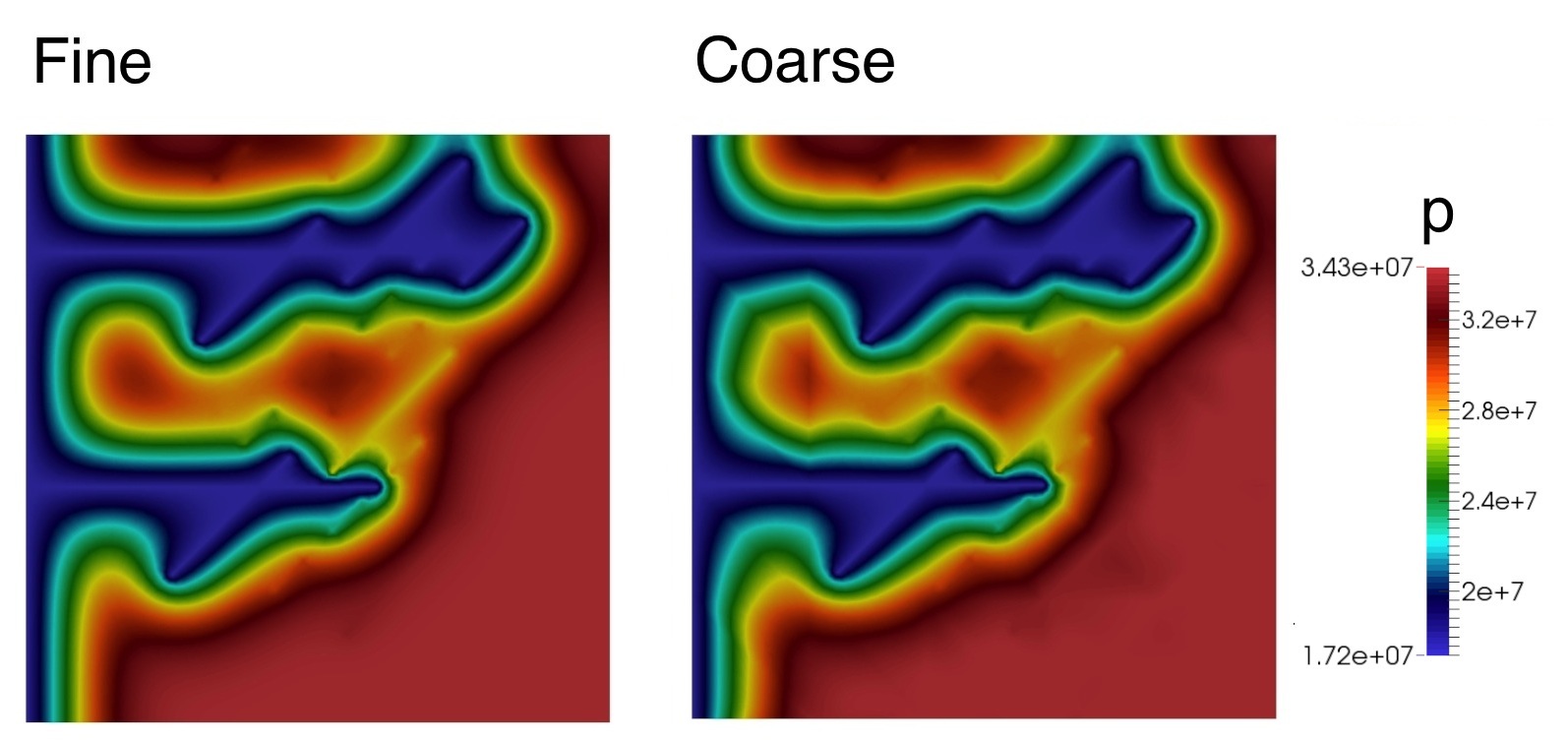
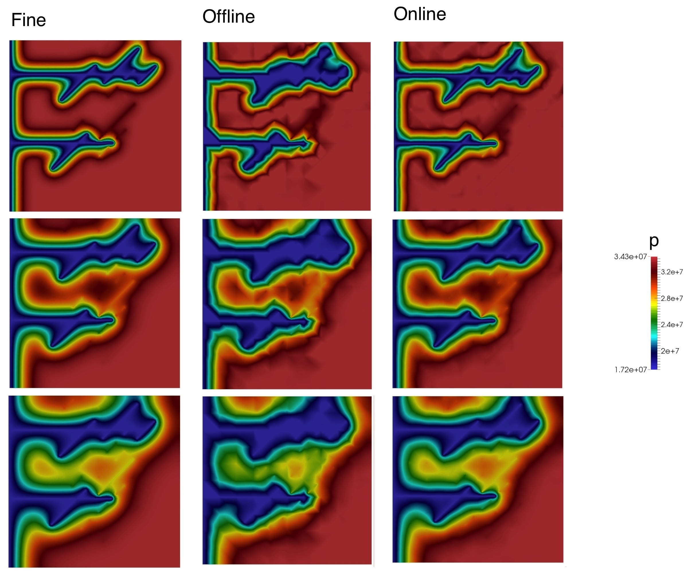
In Figure 5, we show the pressure distribution for three concrete time level $t=1,3$ and $5$ years. For the pressure and concentration, we have the following relationship: $p=RTc$. Pressure distribution for nonlinear matrix-fracture coefficients in (6) is presented in Figures 6 - 7 for last time level. In these figures, we show fine-scale (reference) and coarse-scale (multiscale) solutions. The coarse-scale solution is obtained in an offline space of dimension $288$ (using $M_{off}=8$ multiscale basis functions per coarse neighborhood) and the fine-scale solution is obtained in a space of dimension $3891$. Compared to the fine-scale solution on the left with the coarse-scale solution on the right of the figures, we observe that the GMsFEM can approximate the fine-scale solution accurately.

To compare the results, we use relative weighted errors

$$||\varepsilon||_{*}=||c_{\text{ms}}-c_{h}||_{*}/||c_{h}||_{*},$$

using $L^{2}_{a}$ and $H^{1}_{a}$ weighted norms that are defined as

$$||\varepsilon||_{L^{2}_{a}}=\left(\int_{\Omega}a\,\varepsilon^{2}\,dx\right)^{1/2},\quad||\varepsilon||_{H^{1}_{a}}=\left(\int_{\Omega}(a\,\nabla\varepsilon,\nabla\varepsilon)\,dx\right)^{1/2}.$$

Figure 8: Multiscale basis functions corresponding to the first $3$ smallest eigenvalues in the case with constant fracture-matrix properties after multiplication to partition of unity functions, $\psi_{i,k}=\chi_{i}\psi_{k}^{\omega_{i},\text{off}}$, $i=25$ and $k=0,1,2$ (from left to right)

In Table 1, we present relative errors (in percentage) for last time level for constant fracture and matrix properties in (6) using coarse grids with 36 and 121 nodes. For the coarse-scale approximation, we vary the dimension of the spaces by selecting a certain number of offline basis functions ($M_{off}$) corresponding to the smallest eigenvalues. In the Table 1, we recall that $V_{off}$ denotes the offline space, $dim(V_{off})$ is the offline space dimension, $M_{off}$ is the number of the multiscale basis functions per coarse neighborhood (we use a similar number of $M_{off}$ for each $\omega_{i}$), $c_{\text{ms}}$ and $c_{h}$ are the multiscale and reference solutions, respectively.

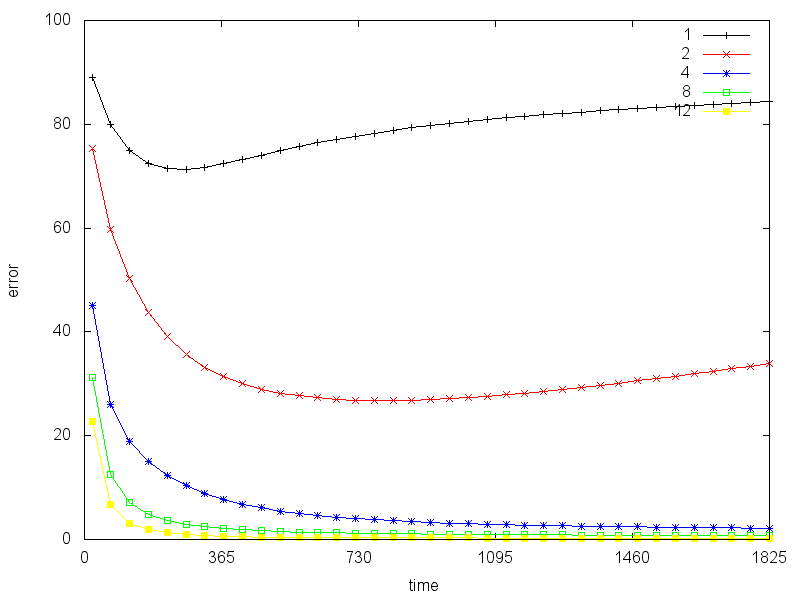
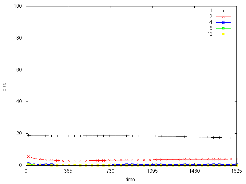
Figure 8 presents the multiscale basis functions corresponding to the first $3$ smallest eigenvalues in the case with constant fracture-matrix properties in (6). These offline basis functions are multiplied by partition of unity functions. When we use $M_{off}=8$ and the case with $36$ coarse nodes, the relative $L^{2}_{a}$ and $H^{1}_{a}$ weighted errors are $0.3$ % and $0.7$%, respectively for final time level. The dimension of the corresponding offline space is $288$ and for reference solution is $3891$. For coarse grid with $121$ nodes, the relative errors are slightly smaller $0.1$% and $0.2$% for $L^{2}_{a}$ and $H^{1}_{a}$ weighted errors, respectively. The dimension of the corresponding offline space is $968$ and for reference solution is $6659$. The relative $L^{2}_{a}$ and $H^{1}_{a}$ errors at different time instants for the cases with $36$ and $121$ coarse grids are presented in Figures 9 and 10. As we observe if we take $4$ or more basis functions per coarse node, the relative errors remain small.

$M_{off}$	dim($V_{off}$)	$\lambda_{min}$	$L^{2}_{a}$	$H^{1}_{a}$
1	36	9.0 10-9	24.484	84.383
2	72	4.5 10-8	12.229	33.923
4	144	1.1 10-7	1.068	2.162
8	288	2.2 10-6	0.303	0.737
12	432	0.19	0.083	0.258

    $M_{off}$ dim($V_{off}$) $\lambda_{min}$ $L^{2}_{a}$ $H^{1}_{a}$ 1 121 2.5 10^-8 17.136 68.989 2 242 9.6 10^-8 3.975 36.337 4 484 1.6 10^-7 0.651 3.595 8 968 0.37 0.110 0.246 12 1452 1.23 0.060 0.108

Table 1: Numerical results (relative errors (%) for the final time level). Left: for the case with $36$ coarse nodes. Right: for the case with $121$ coarse nodes.

Figure 9: Relative $L^{2}_{a}$ and $H^{1}_{a}$ weighted errors (%) for coarse grid in Figure 3 with 36 nodes. Constant matrix-fracture properties.

Figure 10: Relative $L^{2}_{a}$ and $H^{1}_{a}$ weighted errors (%) for coarse grid in Figure 3 with 121 nodes. Constant matrix-fracture properties.

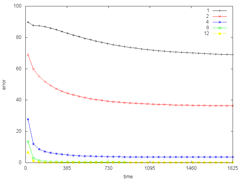
We present relative weighted errors in Tables 2 and 3 for different number of eigenvectors $M_{off}$ for the case with nonlinear matrix-fracture coefficients in (6). We consider a case with $36$ coarse nodes. When we use $M_{off}=8$ and the case with $\kappa=\kappa_{0}$, the relative $L^{2}_{a}$ and $H^{1}_{a}$ errors are $0.2$ % and $0.7$%, respectively. The dimension of the corresponding offline space is $288$ and for reference solution is $3891$. For the case with $\kappa=\kappa_{m}$ in (18), we have $0.4$% and $1.0$% of relative $L^{2}_{a}$ and $H^{1}_{a}$ errors, respectively. The dimension of coarse spaces for the corresponding number of eigenvectors are $72$, $144$, $288$, $432$ and $576$ for $M_{off}=2,4,8$ and $12$. We observe that as the dimension of the coarse space (the number of selected eigenvectors $M_{off}$) increases, the respective relative errors decrease. Also we have similar error behaviour as for case with constant matrix-fracture coefficients. Moreover, we see that the decrease in the relative error is fast initially and one can obtain small errors using only a few basis functions.

$M_{off}$	dim($V_{off}$)	$\lambda_{min}$	$L^{2}_{a}$	$H^{1}_{a}$
1	36	4.8 10-9	21.717	87.897
2	72	2.4 10-8	10.772	38.774
4	144	6.0 10-8	0.933	1.947
8	288	1.1 10-6	0.270	0.737
12	432	0.19	0.123	0.323

    $M_{off}$ dim($V_{off}$) $\lambda_{min}$ $L^{2}_{a}$ $H^{1}_{a}$ 1 121 2.5 10^-8 14.333 64.197 2 242 9.6 10^-8 3.673 30.510 4 484 1.6 10^-7 0.646 3.272 8 968 0.37 0.110 0.251 12 1452 1.23 0.063 0.159

Table 2: Numerical results (relative weighted errors (%) for final time level) for case with $\kappa=\kappa_{0}$ in (18). Left: the case with $36$ coarse nodes. Right: the case with $121$ coarse nodes.

$M_{off}$	dim($V_{off}$)	$\lambda_{min}$	$L^{2}_{a}$	$H^{1}_{a}$
1	36	2.0 10-9	24.484	92.039
2	72	1.0 10-8	10.785	35.874
4	144	2.6 10-8	1.247	2.423
8	288	5.1 10-7	0.432	1.069
12	432	0.19	0.234	0.712

    $M_{off}$ dim($V_{off}$) $\lambda_{min}$ $L^{2}_{a}$ $H^{1}_{a}$ 1 121 2.5 10^-8 16.318 60.267 2 242 9.6 10^-8 3.715 22.872 4 484 1.6 10^-7 0.645 3.000 8 968 0.37 0.134 0.386 12 1452 1.23 0.096 0.282

Table 3: Numerical results (relative weighted errors (%) for the final time level) for case with $\kappa=\kappa_{m}$ in (18). Left: the case with $36$ coarse nodes. Right: the case with $121$ coarse nodes.

Remark 4.1.

In our numerical simulations, we do not use empricial interpolation procedures for approximating the nonlinear functionals $a_{\cdot}(c,\cdot)$ and $b_{\cdot}(c,\cdot)$ (see [6] for more details). In the approaches of [6], empirical interpolation concepts [7] are used to evaluate the nonlinear functions by dividing the computation of the nonlinear function into coarse regions, evaluating the contributions of nonlinear functions in each coarse region taking advantage of a reduced-order representation of the solution. By using these approaches, we can reduce the computational cost associated with evaluating the nonlinear functions and consequently making the computational cost to be independent of the fine grid.

5 Randomized oversampling GMsFEM

Next, we present numerical results for the oversampling and the randomized snapshots that can substantially save the computational cost for snapshot calculations. In this algorithm, instead of solving local harmonic problems (11) for each fine grid node on the boundary, we solve a small number of harmonic extension local problems with random boundary conditions [5]. More precisely, we let

$$\psi_{j}^{\omega_{i},\text{rsnap}}=r_{j},\quad x\in\partial\omega_{i}^{+},$$

where $r_{j}$ are independent identical distributed standard Gaussian random vectors on the fine grid nodes of the boundary. When we use randomized snapshots, we only generate a fraction of the snapshot vectors by using random boundary conditions.

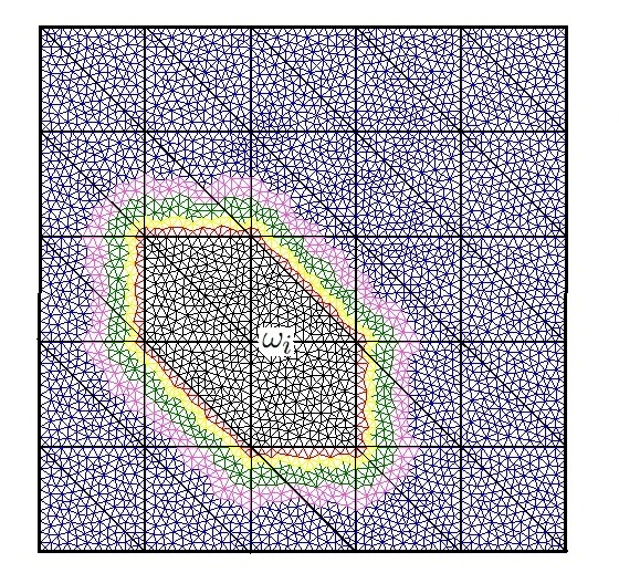
For snapshot space calculations, we use the extended coarse grid neighborhood for $m=1,2,\dots$, by $\omega^{+}_{i}=\omega_{i}+m$, where $m$ is width of the fine-grid layer. Here, for example, $\omega^{+}_{i}=\omega_{i}+1$ means the coarse grid neighborhood plus all 1 layer of adjacent fine grid of $\omega_{i}$, and so on (see Figure 11 for illustration). Calculations in the oversampled neighborhood domain $\omega_{i}^{+}$ reduces the effects due to the artificial oscillation in random boundary conditions.

Figure 11: Neighborhood domain with oversampling ($\omega^{+}_{i}=\omega_{i}+m$, $m=1,2,4,6$) for the coarse grid with 36 nodes

5.1 Numerical results

The simulation results are presented in Tables 4 - 5 for 36 node coarse grid case. We use constant matrix-fracture properties, see (6). We present the results for the randomized snapshot case for last time level. In our simulations, we set the oversampling size $m=0,2,4,6$ for $\omega^{+}_{i}=\omega_{i}+m$ and use different numbers of multiscale basis functions $M_{off}=2,4,8$ and $12$.

In Table 4, we investigate the effects of the oversampling $\omega^{+}_{i}=\omega_{i}+m$, as we increase the number of fine grid extensions $m=0,2,4$ and $6$. We see that the oversampling helps to improve the results initially, but the improvements slow and larger oversampling domains do not give significant improvement in the solution accuracy. When we use a snapshot ratio of $25.6$ % (between the standard number of snapshots and the randomized algorithm for $\omega^{+}_{i}=\omega_{i}+4$), the relative $L^{2}_{a}$ and $H^{1}_{a}$ weighted errors are $0.2$ % and $0.8$% for full snapshots and $0.2$ % and $0.9$% for randomized snapshots. We observe that the randomized algorithm can give similar errors as a full snapshots.

Table 5 shows relative $L^{2}_{a}$ and $H^{1}_{a}$ errors for different number of randomized snapshots $M_{i}$. The oversampled region $\omega^{+}_{i}=\omega_{i}+4$ is chosen, that is, the oversampled region contains an extra $4$ fine-grid cell layers around $\omega_{i}$. Our numerical results show that one can achieve a similar accuracy when using a fraction of snapshots with randomized algorithms and thus, it can provide a substantial CPU savings.

$M_{off}$	full snapshots		randomized snapshots
	$L^{2}_{a}$	$H^{1}_{a}$	$L^{2}_{a}$	$H^{1}_{a}$
without oversampling, $\omega_{i}$
	100 %		39.7 %
2	12.229	33.923	8.303	33.237
4	1.068	2.162	1.704	4.730
8	0.303	0.737	1.005	2.962
12	0.083	0.258	0.557	1.643
with oversampling, $\omega_{i}^{+}=\omega_{i}+2$
	100 %		28.3 %
2	12.247	33.943	8.921	33.399
4	1.073	4.237	0.972	3.750
8	0.261	0.744	0.354	1.003
12	0.114	0.329	0.219	0.704
with oversampling, $\omega_{i}^{+}=\omega_{i}+4$
	100 %		25.6 %
2	12.216	33.657	9.334	28.213
4	1.015	4.576	0.626	2.561
8	0.262	0.841	0.264	0.949
12	0.114	0.349	0.153	0.441
with oversampling, $\omega_{i}^{+}=\omega_{i}+6$
	100 %		22.5 %
2	12.746	35.899	9.455	27.922
4	1.013	5.014	0.603	2.377
8	0.251	0.820	0.277	0.875
12	0.124	0.369	0.120	0.421

Table 4: Randomized oversampling for GMsFEM with number of snapshots $M_{i}=24$ (constant matrix-fracture properties) in every $\omega_{i}^{+}=\omega_{i}+n$, $n=0,2,4,6$ for coarse mesh with 36 nodes (relative errors (%) for final time level)

$M_{off}$	12.8 % ($M_{i}=12$)		17.0 % ($M_{i}=16$)		21.3 % ($M_{i}=20$)		25.6 % ($M_{i}=24$)		29.8 % ($M_{i}=28$)
	$L^{2}$	$H^{1}$	$L^{2}$	$H^{1}$	$L^{2}$	$H^{1}$	$L^{2}$	$H^{1}$	$L^{2}$	$H^{1}$
2	8.228	24.878	9.449	28.895	7.346	22.774	9.334	28.213	9.335	26.973
4	1.908	4.208	1.381	3.581	0.779	2.692	0.626	2.561	0.843	4.439
8	0.861	1.777	0.589	1.563	0.292	1.189	0.264	0.949	0.245	0.894
12	-	-	0.313	0.781	0.217	0.581	0.153	0.441	0.110	0.393

Table 5: Randomized oversampling for GMsFEM with different number of snapshots $M_{i}=12,16,20,24,28$ in every $\omega_{i}^{+}=\omega_{i}+4$ (constant matrix-fracture properties) for coarse mesh with 36 nodes (relative errors (%) for final time level)

6 Residual based adaptive online GMsFEM

In this section, we consider the construction of the online basis functions that are used in some regions adaptively to reduce the error significantly. We follow earlier works [9, 8], which were done for linear time-independent problems. The online basis functions are constructed based on a residual and take into account distant effects. The construction of online basis functions is motivated by the analysis. Using the offline computation, we construct multiscale basis functions that can be used for any input parameters to solve the problem on the coarse grid. The fast convergence due to adding online basis functions depends on the offline space. It is important that the offline space contains some essential features of the solution space. In our numerical simulations, we demonstrate that with a sufficient number of offline basis functions, we can achieve a rapid convergence for the proposed online procedure.

First, we derive the error indicator for the error $(c^{n}-c_{\text{ms}}^{n})$ for time-dependent problem (21) in the energy norm. Furthermore, we use the error indicator to develop an enrichment algorithm. The error indicator gives an estimate of the local error on the coarse grid region $\omega_{i}$ and we can then add basis functions to improve the solution.

We assume, as before, $V$ is the fine-scale finite element space. To find the fine-scale solution $c^{n+1}\in V$, we solve (as before)

$$m(\frac{c^{n+1}-c^{n}}{\tau},v)+a(c^{n+1},v)=(f,v),\quad\forall v\in V$$ (20)

and for multiscale solution $c_{\text{ms}}^{n+1}\in V_{\text{off}}$ we have

$$m(\frac{c_{\text{ms}}^{n+1}-c_{\text{ms}}^{n}}{\tau},v)+a(c_{\text{ms}}^{n+1},v)=(f,v),\quad\forall v\in V_{\text{off}}.$$ (21)

We define a linear functional $r^{n}(v)$ for $n$-th time level by

$$r^{n}(v)=\tau(f,v)-m(c_{\text{ms}}^{n+1}-c_{\text{ms}}^{n},v)-\tau a(c_{\text{ms}}^{n+1},v).$$

Let $\omega_{i}$ be a coarse region and $V_{i}=H^{1}_{0}(\omega_{i})$ then

$$\begin{split}r^{n}_{i}(v)&=\tau\int_{\omega_{i}}fv-\int_{\omega_{i}^{m}}a_{m}\,(c_{\text{ms}}^{n+1}-c_{\text{ms}}^{n})\,v\,dx-\tau\int_{\omega_{i}^{m}}b_{m}\,\nabla c_{\text{ms}}^{n+1}\cdot\nabla v\,dx\\ &-d_{j}\sum\limits_{j}\int_{\omega^{f,j}_{i}}a_{f}(c)\,(c_{\text{ms}}^{n+1}-c_{\text{ms}}^{n})\,v\,dx-\tau\,d_{j}\sum\limits_{j}\int_{\omega^{f,j}_{i}}b_{f}\,\nabla c_{\text{ms}}^{n+1}\cdot\nabla v\,dx,\end{split}$$

where $\omega_{i}=\omega_{i}^{m}\oplus_{j}\,d_{j}\omega_{i}^{f,j}$ and $m$ and $f$ represent the matrix and the fracture.

The solution at $(n+1)$ time level ($c_{\text{ms}}^{n+1}$) is the solution of the elliptic problem of the form

$$a_{\tau}(c^{n+1}_{\text{ms}},v)=\tau(f,v)+m(c^{n}_{\text{ms}},v).$$ (22)

We use following notation

$$a_{\tau}(u,v)=m(u,v)+\tau a(u,v).$$

Error estimators for the spatial discretization error take into account the dependence of the elliptic problem (22) on the time step parameter $\tau$ and we will use the $\tau$-weighted $H_{1}$ norm

$$||v||^{2}_{\tau}=\tau||v||_{a}^{2}+||v||^{2}_{m},$$

where

$$||v||^{2}_{\tau}=a_{\tau}(v,v),\quad||v||^{2}_{a}=a(v,v),\quad||v||^{2}_{m}=m(v,v).$$

We define the projection $\Pi:V\rightarrow V_{off}$ by

$$\Pi v=\sum_{i=0}^{N}\chi_{i}(P_{i}v),$$

where $P_{i}:V\rightarrow\text{span}\{\psi_{k}^{w_{i},off}\}$ be the projection defined by

$$P_{i}v=\sum_{k=1}^{l_{i}}\left(b\,v\,\psi_{k}^{w_{i},off}\right)\psi_{k}^{w_{i},off}.$$

The projection $P_{i}$ is the first $l_{i}$ terms of spectral expansion in terms of eigenfunctions of following problem

$$a_{\tau}^{\omega_{i}}(\Psi^{\text{off}},v)=\lambda^{\text{off}}\tau\int_{\omega_{i}}b\,|\nabla\chi_{i}|^{2}\,\Psi^{\text{off}}\,v\,dx.$$ (23)

Then

$$\tau\int_{\omega_{i}}b\,|\nabla\chi_{i}|^{2}\,(v-P_{i}v)^{2}\,dx\leq\frac{1}{\lambda_{l_{i+1}}}a_{\tau}^{\omega_{i}}(v-P_{i}v,v-P_{i}v).$$

and

$$a_{\tau}^{\omega_{i}}(v-P_{i}v,v-P_{i}v)\leq a_{\tau}^{\omega_{i}}(v,v).$$

We note that this spectral problem is different from the original one formulated in (12); however, it involves similar terms, such as energy norms and $L^{2}$ norms.

Let $e^{n}=c^{n}-c_{\text{ms}}^{n}$ is error for $n$-th time level and using (20) and (21), we have

$$m(e^{n+1}-e^{n},v)+\tau a(e^{n+1},v)=(r^{n},v),$$ (24)

where the right hand side can be written as follows

$$\begin{split}r^{n}(v)&=\tau(f,v)-m(c_{\text{ms}}^{n+1}-c_{\text{ms}}^{n},v)-\tau a(c_{\text{ms}}^{n+1},v)\\ &\leq\tau(f,v-\Pi v)+\tau(f,\Pi v)-m(c_{\text{ms}}^{n+1}-c_{\text{ms}}^{n},\Pi v)-\tau a(c_{\text{ms}}^{n+1},\Pi v)\\ &-m(c_{\text{ms}}^{n+1}-c_{\text{ms}}^{n},v-\Pi v)-\tau a(c_{\text{ms}}^{n+1},v-\Pi v)\\ &=\tau(f,v-\Pi v)-m(c_{\text{ms}}^{n+1}-c_{\text{ms}}^{n},v-\Pi v)-\tau a(c_{\text{ms}}^{n+1},v-\Pi v)\\ &=\sum_{i=1}^{N}r_{i}^{n}\left(\chi_{i}(v-P_{i}v)\right)\leq\sum_{i=1}^{N}||r_{i}^{n}||_{*}||\chi_{i}(v-P_{i}v)||_{\tau}.\end{split}$$

We have

$$\begin{split}||\chi_{i}(v-P_{i}v)||_{\tau}^{2}&=||\chi_{i}(v-P_{i}v)||_{m}^{2}+\tau||\chi_{i}(v-P_{i}v)||_{a}^{2}\\ &=||\chi_{i}(v-P_{i}v)||_{m}^{2}+\tau C\int_{\omega_{i}}b\,|\nabla\chi_{i}|^{2}\,(v-P_{i}v)^{2}\,dx+\tau C\int_{\omega_{i}}b\,\chi_{i}^{2}\,|\nabla(v-P_{i}v)|^{2}\,dx\\ &\leq Ca_{\tau}^{\omega_{i}}(v-P_{i}v,v-P_{i}v)+\tau C\int_{\omega_{i}}b\,|\nabla\chi_{i}|^{2}\,(v-P_{i}v)^{2}\,dx\\ &\leq\left(C+\frac{C}{\lambda_{l_{i+1}}}\right)a_{\tau}^{\omega_{i}}(v-P_{i}v,v-P_{i}v)\leq\left(C+\frac{C}{\lambda_{l_{i+1}}}\right)a_{\tau}^{\omega_{i}}(v,v).\end{split}$$ (25)

Therefore

$$\begin{split}m(e^{n+1}-e^{n},v)&+\tau a(e^{n+1},v)\leq\sum_{i=1}^{N}||r_{i}^{n}||_{*}||\chi_{i}(v-P_{i}v)||_{\tau}\leq\sum_{i=1}^{N}||r_{i}^{n}||_{*}\left(C+\frac{C}{\lambda_{l_{i+1}}}\right)^{1/2}a_{\tau}^{\omega_{i}}(v,v)^{1/2}\\ &\leq\left(C+\frac{C}{\Lambda_{min}}\right)^{1/2}\left(\sum_{i=1}^{N}||r_{i}^{n}||_{*}^{2}\right)^{1/2}\sum_{i=1}^{N}a_{\tau}^{\omega_{i}}(v,v)^{1/2}\leq\left(C+\frac{C}{\Lambda_{min}}\right)^{1/2}\left(\sum_{i=1}^{N}||r_{i}^{n}||_{*}^{2}\right)^{1/2}a_{\tau}(v,v)^{1/2},\end{split}$$

where $\Lambda_{min}=\min_{i}\lambda_{l_{i+1}}$.

Finally, we take $v=e^{n+1}$

$$\begin{split}||e^{n+1}||^{2}_{\tau}&\leq\left(C+\frac{C}{\Lambda_{min}}\right)^{1/2}\left(\sum_{i=1}^{N}||r_{i}^{n}||_{*}^{2}\right)^{1/2}||e^{n+1}||_{\tau}+m(e^{n},e^{n+1})\\ &\leq\left(C+\frac{C}{\Lambda_{min}}\right)^{1/2}\left(\sum_{i=1}^{N}||r_{i}^{n}||_{*}^{2}\right)^{1/2}||e^{n+1}||_{\tau}+||e^{n}||_{m}||e^{n+1}||_{\tau}.\end{split}$$

Then

$$||e^{n+1}||_{\tau}\leq\left(C+\frac{C}{\Lambda_{min}}\right)^{1/2}\left(\sum_{i=1}^{N}||r_{i}^{n}||_{*}^{2}\right)^{1/2}+||e^{n}||_{m}.$$

This inequality residuals give a computable indicator of the error $e^{n+1}=c^{n+1}-c_{\text{ms}}^{n+1}$ in the $\tau$-weighted $H_{1}$ norm.

Remark 6.1.

We note that the analysis suggests the use of (23) as a local eigenvalue problem. This eigenvalue problem is “slightly” different from (12) that we have used earlier. Our numerical simulations show that the use of (23) improves the convergence of the offline or online procedures slightly in our numerical examples. We will use the spectral problems based on (12) in our numerical simulations as it is independent of time stepping.

Next, we consider online basis construction. We use the index $m\geq 1$ to represent the enrichment level. At the enrichment level $m$, we use $V^{m}_{\text{ms}}$ to denote the corresponding space that can contains both offline and online basis functions. We will consider a strategy for getting the space $V^{m+1}_{\text{ms}}$ from $V^{m}_{\text{ms}}$. By the online basis functions we mean basis functions that are computed during iterative process, contrary to offline basis functions that are computed before iterative process. The online basis functions are computed based on some local residuals for the current multiscale solution $c_{\text{ms}}^{n+1,(m)}$.

Let $V^{m+1}_{\text{ms}}=V^{m}_{\text{ms}}+\text{span}\{\varphi\}$ be the new approximate space that constructed by adding online basis $\varphi\in V_{i}$ on the $i$-th coarse neighborhood $\omega_{i}$ and $c_{\text{ms}}^{n+1,(m+1)}\in V^{m+1}_{\text{ms}}$ be the corresponding GMsFEM solution.

We define $c_{\text{semi}}^{n+1}=c_{\text{semi}}^{n+1}(c_{\text{ms}}^{n,(m)})$, which satisfies

$$a_{\tau}(c_{\text{semi}}^{n+1},v)=\tau(f,v)+m(c^{n}_{\text{ms}},v).$$

For the error $c_{\text{ms}}^{n+1}-c_{\text{semi}}^{n+1}$, we have

$$\begin{split}a_{\tau}(c_{\text{ms}}^{n+1}-c_{\text{semi}}^{n+1},c_{\text{ms}}^{n+1}-c_{\text{semi}}^{n+1})&=a_{\tau}(c_{\text{ms}}^{n+1},c_{\text{ms}}^{n+1}-c_{\text{semi}}^{n+1})-a_{\tau}(c_{\text{semi}}^{n+1},c_{\text{ms}}^{n+1}-c_{\text{semi}}^{n+1})\\ &=a_{\tau}(c_{\text{ms}}^{n+1},c_{\text{ms}}^{n+1}-c_{\text{semi}}^{n+1})-(\tau f,c_{\text{ms}}^{n+1}-c_{\text{semi}}^{n+1})-m(c_{\text{ms}}^{n},c_{\text{ms}}^{n+1}-c_{\text{semi}}^{n+1})\\ &=r(c_{\text{ms}}^{n+1}-c_{\text{semi}}^{n+1})=\sum_{i}^{N}r_{i}(\chi_{i}(P_{i}(c_{\text{semi}}^{n+1}-c_{\text{ms}}^{n+1})+c_{\text{ms}}^{n+1}-c_{\text{semi}}^{n+1}))\\ &\leq\sum_{i}^{N}||r_{i}||_{*}||\chi_{i}(P_{i}(c_{\text{semi}}^{n+1}-c_{\text{ms}}^{n+1})+c_{\text{ms}}^{n+1}-c_{\text{semi}}^{n+1})||_{\tau}.\end{split}$$

Using (25) we obtain

$$a_{\tau}(c_{\text{ms}}^{n+1}-c_{\text{semi}}^{n+1},c_{\text{ms}}^{n+1}-c_{\text{semi}}^{n+1})\leq\left(C+\frac{C}{\Lambda_{min}}\right)\sum_{i}^{N}||r_{i}||_{*}.$$ (26)

The solution $c_{\text{ms}}^{n+1,(m+1)}$ satisfies

$$||c_{\text{ms}}^{n+1,(m+1)}-c_{\text{semi}}^{n+1}||_{\tau}^{2}\leq||v-c_{\text{semi}}^{n+1}||_{\tau}^{2},\quad\forall v\in V_{\text{ms}}^{m+1}.$$

Taking $v=c_{\text{ms}}^{n+1,(m)}+\alpha\varphi$, we have

$$||c_{\text{ms}}^{n+1,(m+1)}-c_{\text{semi}}^{n+1}||_{\tau}^{2}\leq||c_{\text{ms}}^{n+1,(m)}+\alpha\varphi-c_{\text{semi}}^{n+1}||_{\tau}^{2}=||c_{\text{ms}}^{n+1,(m)}-c_{\text{semi}}^{n+1}||_{\tau}^{2}+2\alpha\,a_{\tau}^{\omega_{i}}(c_{\text{ms}}^{n+1,(m)}-c_{\text{semi}}^{n+1},\varphi)+\alpha^{2}a_{\tau}^{\omega_{i}}(\varphi,\varphi).$$

The last two terms in above inequality measure the amount of the reduction in error when the new basis function $\varphi$ is added to the space $V_{\text{ms}}^{m}$.

For $\alpha=-1$ and $\varphi\in V_{i}$ is the solution of

$$a_{\tau}(\varphi,v)=r(v),\quad\forall v\in V_{i}.$$

Then for $e_{\text{semi}}^{n+1,(m+1)}=c_{\text{ms}}^{n+1,(m+1)}-c_{\text{semi}}^{n+1}$ we have

$$\begin{split}||e_{\text{semi}}^{n+1,(m+1)}||_{\tau}^{2}&\leq||e_{\text{semi}}^{n+1,(m)}||_{\tau}^{2}-2\,a_{\tau}^{\omega_{i}}(c_{\text{ms}}^{n+1,(m)}-c_{\text{semi}}^{n+1},\varphi)+r_{i}(\varphi)\\ &\leq||e_{\text{semi}}^{n+1,(m)}||_{\tau}^{2}-2\,a_{\tau}^{\omega_{i}}(c_{\text{ms}}^{n+1,(m)},\varphi)+2\tau(f,v)+2m(c^{n,(m)}_{\text{ms}},\varphi)+r(\varphi)\leq||e_{\text{semi}}^{n+1,(m)}||_{\tau}^{2}-||r||_{*}^{2}.\end{split}$$

To enhance the convergence and efficiency of the online adaptive GMsFEM, we consider enrichment on non-overlapping coarse neighbothoods. Let $I\subset\{1,2,\dots,N\}$ be the index set of some non-overlapping coarse neighborhoods. We define $V^{m+1}_{\text{ms}}=V^{m}_{\text{ms}}+\text{span}\{\varphi_{i},\,\i\in I\}$ and obtain

$$||e_{\text{semi}}^{n+1,(m+1)}||_{\tau}^{2}\leq||e_{\text{semi}}^{n+1,(m)}||_{\tau}^{2}-\sum_{i\in I}||r_{i}||_{*}^{2}.$$

Finally, we combine this with (26) and obtain

$$\begin{split}||e_{\text{semi}}^{n+1,(m+1)}||_{\tau}^{2}&\leq||e_{\text{semi}}^{n+1,(m)}||_{\tau}^{2}-\sum_{i\in I}||r_{i}||^{2}_{*}\frac{a_{\tau}^{\omega_{i}}(e_{\text{semi}}^{n+1,(m)},e_{\text{semi}}^{n+1,(m)})}{\left(C+\frac{C}{\Lambda_{min}}\right)\sum_{i=1}^{N}||r_{i}||_{*}^{2}}\\ &\leq\left(1-\frac{\sum_{i\in I}||r_{i}||^{2}_{*}}{\left(C+\frac{C}{\Lambda_{min}}\right)\sum_{i=1}^{N}||r_{i}||_{*}^{2}}\right)||e_{\text{semi}}^{n+1,(m)}||_{\tau}^{2}.\end{split}$$

We will find online basis functions $\varphi\in V_{i}$ to maximize the local resudial $r^{n}_{i}$ for current time level. Moreover, the required $\varphi$ is the solution of

$$a_{\tau}(\varphi,v)=r_{i}(v),\quad\forall v\in V_{i},$$ (27)

where $R_{i}(v)$is the local residual that defined using $w_{\text{ms}}^{m}$

$$r_{i}(v)=\tau(f,v)-m(c_{\text{ms}}^{n+1}-c_{\text{ms}}^{n},v)-\tau a(c_{\text{ms}}^{n+1},v)$$

and $||r_{i}||^{2}_{*}=||\varphi||^{2}_{\tau}$ according to the Riez representation theorem.

For solution in each time level, we iteratively enrich our offline space by residual based online basis function. These basis functions are calculated using Equation (27) with zero Dirichlet boundary conditions and the residual norm $||r^{n}_{i}||_{*}$ provides a measure on the amount of reduction in energy error.

For the construction of the adaptive online basis functions, we first choose $0<\theta<1$, for each coarse neighborhood $\omega_{i}$, find the online basis $\varphi_{i}\in V_{i}$ using equation (27). After compute the norm of local residuals and calculate $\eta_{i}$

$$\eta^{2}_{i}:=\lVert r_{i}\rVert_{\star}^{2},$$

where $\lVert r_{i}\rVert_{\star}=\lVert\phi_{i}\rVert_{\tau}$, then arrange them in descending order, i.e. $\eta^{2}_{1}\geq\eta^{2}_{2}\geq...\geq\eta^{2}_{N}$. Then, choose the smallest $k$ such that

$$\theta\sum_{i=1}^{N}\eta^{2}_{i}\leq\sum_{i=1}^{k}\eta^{2}_{i}.$$

This implies that, for the coarse neighborhood $\omega_{j}(j=1,...k)$, we add the corresponding online basis $\varphi_{j}$ to the original space $V_{ms}^{m}$.

6.1 Numerical results

Next, we present numerical results for residual based online basis functions. We consider a similar problem as in the previous section with constant matrix-fracture properties in (6) and iteratively enrich the offline space by online residual basis functions in some selected time steps. Our coarse and fine grid setups are the same as in Section 4.1. Because re-generation of the matrix $R$ is needed, when we add online basis function, we add them for some selected time steps. We note that, when we add new online basis functions, which are based on current residuals, we remove previously calculated online basis function and keep them till we update the online basis functions. It will save computational time if we have small size of coarse scale problem.

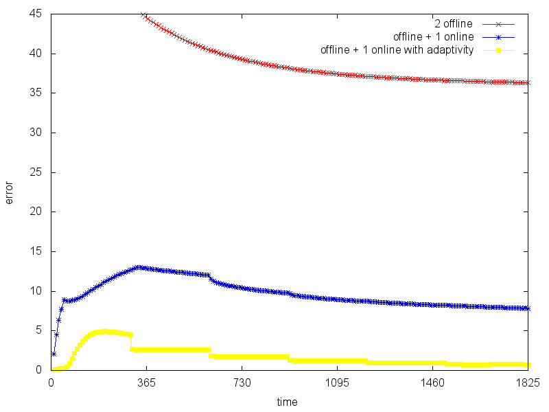
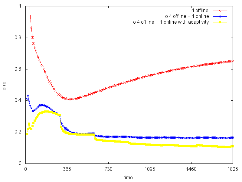
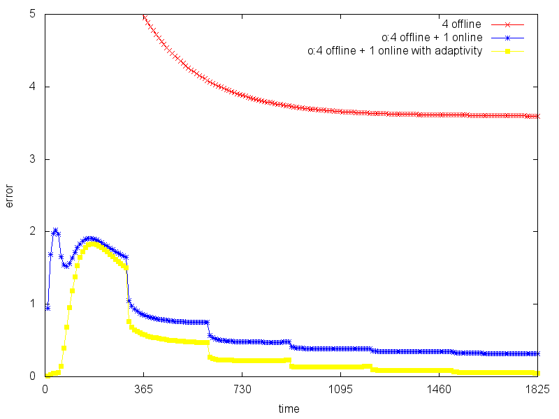
In Table 6, we present $L^{2}_{a}$ and $H^{1}_{a}$ errors. We consider three different cases. In the first case (we call it Case 1), online basis functions are added at the first time step and after that in every $30$-th time step. In the second case (we call it Case 2), online basis functions are replaced at the first five consecutive time steps, and after that, the online basis functions are updated in every $30$-th time step. In the third case (we call it Case 3), online basis functions are replaced at the first ten consecutive time steps, and after that, the online basis functions are updated in every $30$-th time step. More updates initially helps to reduce the error due to the initial condition. As we mentioned that the offline space is important for the convergence, and we present the results for different number of initial offline basis functions per coarse neighborhood. We use multiscale basis functions from offline space as a initial basis functions. In Table 7, we show errors when online basis functions are replaced at the first five consecutive time steps (as in Case 2), and afterwards, online basis functions are updated at $10$-th, $20$-th and $30$-th time step. For our calculations, we use $t_{max}=5$ years with $\tau=10$ days. Calculations are performed in the coarse grid with 121 nodes for the case with constant matrix-fracture properties. We observe from this table the following facts.

• Choosing $4$ initial offline basis functions improves the convergence substantially. This indicates that the choice of the initial offline space is important.

• Adding online basis functions less frequently (such as at every $30$th time step) provides an accurate approximation of the solution. This indicates that the online basis functions can be added only at some selected time steps.

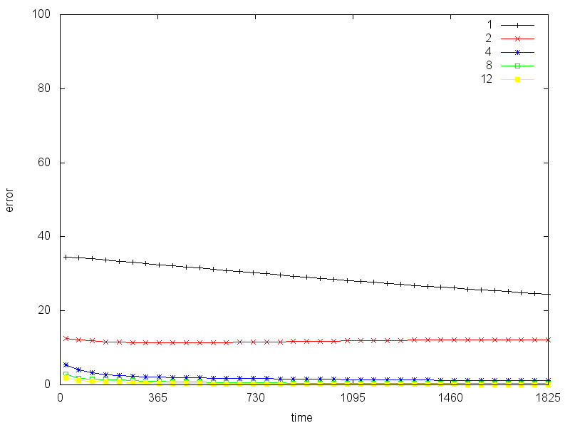
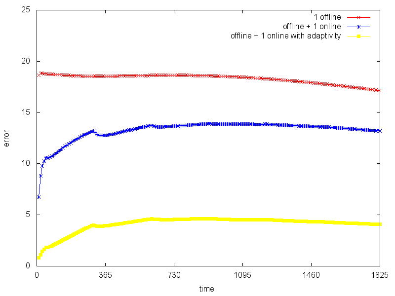
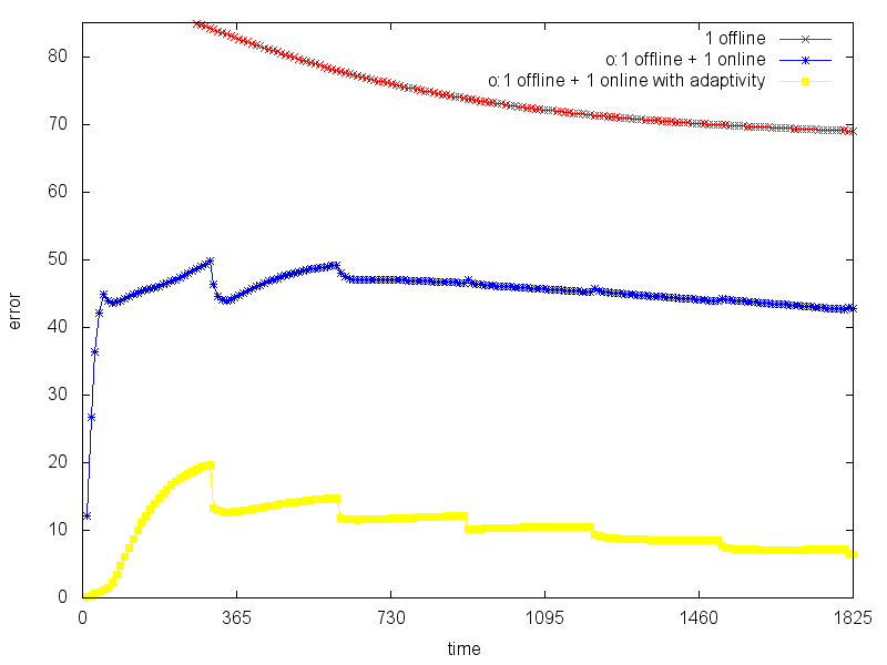
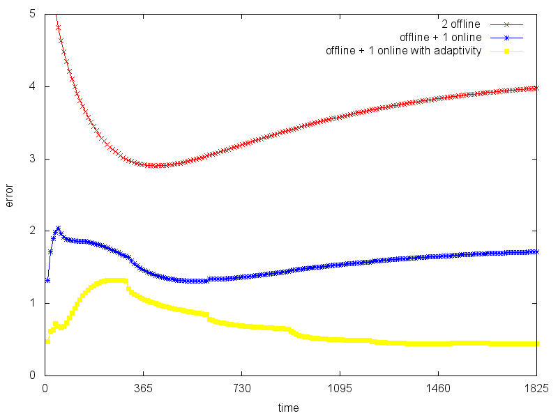
Next, we would like to show that one can use online basis functions adaptively and use the adaptivity criteria discussed above. In Table 8, we present results for residual based online basis functions with adaptivity with $\theta=0.7$. In Figure 13, we show errors by time. We observe that applying adaptive algorithm can much reduce errors.

Figure 12: Fine scale solution (right), coarse-scale using 2 offline basis functions (middle) and coarse-scale after two online iteration for some time levels (left) for t=1, 3 and 5 year (from top to bottom) (constant matrix-fracture coefficients). For fine-scale solution size of problem is 6659. For 2 offline basis functions is 242 and after two online iteration is 484

$DOF$	$L^{2}_{a}$	$H^{1}_{a}$
(# iter)
$M_{off}=1$
121	17.136	68.989
242 (1)	13.047	43.662
363 (2)	7.275	12.262
$M_{off}=2$
242	3.975	36.337
363 (1)	1.653	6.705
484 (2)	0.889	0.972
$M_{off}=4$
484	0.651	3.595
605 (1)	0.208	0.307
726 (2)	0.171	0.056

    $DOF$ $L^{2}_{a}$ $H^{1}_{a}$ (# iter) $M_{off}=1$ 121 17.136 68.989 242 (1) 13.209 42.777 363 (2) 6.603 12.689 $M_{off}=2$ 242 3.975 36.337 363 (1) 1.716 7.841 484 (2) 0.546 0.914 $M_{off}=4$ 484 0.651 3.595 605 (1) 0.165 0.313 726 (2) 0.105 0.057     $DOF$ $L^{2}_{a}$ $H^{1}_{a}$ (# iter) $M_{off}=1$ 121 17.136 68.989 242 (1) 13.002 42.091 363 (2) 6.125 13.186 $M_{off}=2$ 242 3.975 36.337 363 (1) 1.692 8.709 484 (2) 0.449 0.862 $M_{off}=4$ 484 0.651 3.595 605 (1) 0.144 0.318 726 (2) 0.076 0.056

Table 6: Convergence history using one, two and four offline basis functions ($M_{off}=1,2$ and 4). We add online basis functions for every 30 time step and for $N-$th first steps (Cases 1, 2, and 3). Left: $N=1$. Middle: $N=5$. Right: $N=10$. Here $DOF$ for the last time step.

$DOF$	$L^{2}_{a}$	$H^{1}_{a}$
(# iter)
$M_{off}=1$
121	17.136	68.989
242 (1)	12.511	41.477
363 (2)	5.910	13.153
$M_{off}=2$
242	3.975	36.337
363 (1)	1.624	8.225
484 (2)	0.378	0.934
$M_{off}=4$
484	0.651	3.595
605 (1)	0.126	0.303
726 (2)	0.048	0.033

    $DOF$ $L^{2}_{a}$ $H^{1}_{a}$ (# iter) $M_{off}=1$ 121 17.136 68.989 242 (1) 12.925 42.778 363 (2) 6.275 12.705 $M_{off}=2$ 242 3.975 36.337 363 (1) 1.669 8.034 484 (2) 0.474 0.880 $M_{off}=4$ 484 0.651 3.595 605 (1) 0.147 0.305 726 (2) 0.080 0.041     $DOF$ $L^{2}_{a}$ $H^{1}_{a}$ (# iter) $M_{off}=1$ 121 17.136 68.989 242 (1) 13.209 42.777 363 (2) 6.603 12.689 $M_{off}=2$ 242 3.975 36.337 363 (1) 1.716 7.841 484 (2) 0.546 0.914 $M_{off}=4$ 484 0.651 3.595 605 (1) 0.165 0.313 726 (2) 0.105 0.057

Table 7: Convergence history using one, two and four offline basis functions ($M_{off}=1,2$ and $4$). We add online basis functions for every $N$th time step and for first $5$ steps Left: $N=10$. Middle: $N=20$. Right: $N=30$. Here $DOF$ for last time step

$DOF$	$\sum$ iter	$L^{2}_{a}$	$H^{1}_{a}$
(# iter)
$M_{off}=1$
121		17.136	68.989
242 (1)	11	13.209	42.777
363 (2)	22	6.603	12.689
$M_{off}=2$
242		3.975	36.337
363 (1)	11	1.716	7.841
484 (2)	22	0.546	0.914
$M_{off}=4$
484		0.651	3.595
605 (1)	11	0.165	0.313
726 (2)	22	0.105	0.057

    $DOF$ $\sum$ iter $L^{2}_{a}$ $H^{1}_{a}$ $M_{off}=1$ 121 17.136 68.989 243 44 4.082 6.418 381 78 2.681 2.871 $M_{off}=2$ 242 3.975 36.337 376 44 0.441 0.720 504 77 0.376 0.325 $M_{off}=4$ 484 0.651 3.595 635 44 0.110 0.044 737 68 0.098 0.039

Table 8: Convergence history using one, two and four offline basis functions ($M_{off}=1,2$ and 4). We add online basis functions for every 30 time step and for first 5 steps Left: without space adaptivity. Right: with space adaptivity. Here $DOF$ for last time step

Figure 13: Dynamic of relative $L^{2}_{a}$ (left) and $H^{1}_{a}$ (right) weighted errors (%) for coarse grid in figure 4 with 121 nodes for the case with constant coefficients. Weighted errors using offline basis functions and online basis functions with and without adaptivity. Top: 1 offline basis function. Middle: 2 offline basis functions. Bottom: 4 offline basis functions.

7 Conclusions

In this paper, we present a multiscale approach for shale transport in fractured media. Our approach uses an upscaled model in the form of nonlinear parabolic equations to represent the matrix that consists of organic and inorganic matter. The nonlinearities in the equation are due to the interaction of organic and inorganic matter. The interaction of nonlinear matrix and the fracture is represented by multiscale basis functions. We follow Generalized Multiscale Finite Element Method to extract the leading order terms that represent the matrix and the fracture interaction. Multiscale basis functions are constructed locally in each coarse region and they represent the interaction between the upscaled matrix and the fracture network. We show that our proposed approach can effectively capture the small-scale effects and the overall system can be modeled using a fewer degrees of freedom. Numerical results are presented. In some cases and some regions, the offline procedure is insufficient to give accurate representations of the solution, due to the fact that offline computations are typically performed locally and global information is missing in these offline information. These phenomena occur locally and in some of these regions that are identified using the proposed error indicators, we need to develop online basis functions [8]. We discuss online basis functions and show that this procedure converges fast.

8 Acknowledgements

We are grateful to Tat Leung for helpful discussions and suggestions regarding to online basis constructions. MV’s work is partially supported by Russian Science Foundation Grant RS 15-11-10024.

References

- [1] I Yucel Akkutlu, Yalchin Efendiev, and Viktoria Savatorova. Multi-scale asymptotic analysis of gas transport in shale matrix. Transport in Porous Media, 107(1):235–260, 2015.
- [2] I Yucel Akkutlu and Ebrahim Fathi. Multiscale gas transport in shales with local kerogen heterogeneities. SPE Journal, 17(04):1–002, 2012.
- [3] Raymond J Ambrose, Robert C Hartman, Mery Diaz-Campos, I Yucel Akkutlu, Carl H Sondergeld, et al. Shale gas-in-place calculations part i: New pore-scale considerations. SPE Journal, 17(01):219–229, 2012.
- [4] R. Baca, R. Arnett, and D. Langford. Modeling fluid flow in fractured porous rock masses by finite element techniques. Int. J. Num., 4:337–348, 1984.
- [5] V. Calo, Y. Efendiev, J. Galvis, and G. Li. Randomized oversampling for generalized multiscale finite element methods. http://arxiv.org/pdf/1409.7114.pdf.
- [6] Victor M Calo, Yalchin Efendiev, Juan Galvis, and Mehdi Ghommem. Multiscale empirical interpolation for solving nonlinear pdes. Journal of Computational Physics, 278:204–220, 2014.
- [7] S. Chaturantabut and D. C. Sorensen. Application of pod and deim to dimension reduction of nonlinear miscible viscous fingering in porous media. Mathematical and Computer Modeling of Dynamical Systems, 17:337–353, 2011.
- [8] Eric T Chung, Yalchin Efendiev, and Wing Tat Leung. Residual-driven online generalized multiscale finite element methods. arXiv preprint arXiv:1501.04565, 2015.
- [9] E.T. Chung, Y. Efendiev, and G. Li. An adaptive GMsFEM for high-contrast flow problems. Journal of Computational Physics, 273:54–76, 2014.
- [10] Peter Dietrich, Rainer Helmig, Martin Sauter, Heinz Hötzl, Jürgen Köngeter, and Georg Teutsch. Flow and transport in fractured porous media. Springer Science & Business Media, 2005.
- [11] L. J. Durlofsky. Numerical calculation of equivalent grid bock permeability tensors for heterogeneous porous media. Water resources research, 27(5):699–708, 1991.
- [12] Y. Efendiev, J. Galvis, and E. Gildin. Local-global multiscale model reduction for flows in highly heterogeneous media. Journal of Computational Physivs, 231 (24):8100–8113, 2012.
- [13] Y. Efendiev, J. Galvis, and T. Hou. Generalized multiscale finite element methods. Journal of Computational Physics, 251:116–135, 2013.
- [14] Y. Efendiev, J. Galvis, G. Li, and M. Presho. Generalized multiscale finite element methods. oversampling strategies. International Journal for Multiscale Computational Engineering, accepted, 2013.
- [15] Y. Efendiev, J. Galvis, and X.H. Wu. Multiscale finite element methods for high-contrast problems using local spectral basis functions. Journal of Computational Physics, 230:937–955, 2011.
- [16] Y. Efendiev, T. Hou, and V. Ginting. Multiscale finite element methods for nonlinear problems and their applications. Comm. Math. Sci., 2:553–589, 2004.
- [17] Yalchin Efendiev, Seong Lee, Guanglian Li, Jun Yao, and Na Zhang. Hierarchical multiscale modeling for flows in fractured media using generalized multiscale finite element method. arXiv preprint arXiv:1502.03828, 2015. to appear in International Journal on Geomathematics, (DOI) 10.1007/s13137-015-0075-7.
- [18] Anthony F Gangi. Variation of whole and fractured porous rock permeability with confining pressure. In International Journal of Rock Mechanics and Mining Sciences & Geomechanics Abstracts, volume 15, pages 249–257. Elsevier, 1978.
- [19] B. Gong, M. Karimi-Fard, and L. J. Durlofsky. Upscaling discrete fracture characterizations to dual-porosity, dual-permeability models for efficient simulation of flow with strong gravitational effects. SPE J., 13(1):58–67, 2008.
- [20] H. Hajibeygi, D. Karvounis, and P. Jenny. A loosely coupled hierarchical fracture model for the iterative multiscale finite volume method. Society of Petroleum Engineers. doi:10.2118/141991-MS.
- [21] Hadi Hajibeygi, Dimitris Karvounis, Patrick Jenny, et al. A loosely coupled hierarchical fracture model for the iterative multiscale finite volume method. In SPE Reservoir Simulation Symposium. Society of Petroleum Engineers, 2011.
- [22] SH Lee, C Jensen, and I Lunati. Modeling and simulation of shale gas production in multi-staged hydraulic-fractured formations. In ECMOR XIII-13th European Conference on the Mathematics of Oil Recovery, 2012.
- [23] S.H. Lee, M.F. Lough, and C.L. Jensen. Hierarchical modeling of flow in naturally fractured formations with multiple length scales. Water resources research, 37(3):443–455, 2001.
- [24] Jianfang Li, Cong Wang, Didier Ding, Yu-Shu Wu, Yuan Di, et al. A generalized framework model for simulation of gas production in unconventional gas reservoirs. In Paper SPE 163609 presented at SPE Reservoir Simulation Symposium, The Woodlands, Texas, USA, pages 18–20, 2013.
- [25] L. Li and S. H. Lee. Efficient field-scale simulation of black oil in naturally fractured reservoir through discrete fracture networks and homogenized media. SPE Reservoir Evaluation & Engineering.
- [26] Robert G Loucks, Robert M Reed, Stephen C Ruppel, and Daniel M Jarvie. Morphology, genesis, and distribution of nanometer-scale pores in siliceous mudstones of the mississippian barnett shale. Journal of Sedimentary Research, 79(12):848–861, 2009.
- [27] M. F. Lough, S. H. Lee, and J. Kamath. A new method to calculate effective permeability of gridblocks used in the simulation of naturally fractured reservoirs. SPE doi:10.2118/36730-PA.
- [28] M. M. Karimi-Fard and A. Firoozabadi. Numerical simulation of water injection in 2d fractured media using discrete-fracture model. SPE REE J., 4:117–126, 2003.
- [29] J. Noorishad and M. Mehran. An upstream finite element method for solution of transient transport equation in fractured porous media. Water Resour. Res., 18(3):588–596, 1982.
- [30] Volker Reichenberger, Hartmut Jakobs, Peter Bastian, and Rainer Helmig. A mixed-dimensional finite volume method for two-phase flow in fractured porous media. Advances in Water Resources, 29(7):1020–1036, 2006.
- [31] Carl H Sondergeld, Raymond Joseph Ambrose, Chandra Shekhar Rai, Jason Moncrieff, et al. Micro-structural studies of gas shales. In SPE Unconventional Gas Conference. Society of Petroleum Engineers, 2010.
- [32] Asana Wasaki, I Yucel Akkutlu, et al. Permeability of organic-rich shale. In SPE Annual Technical Conference and Exhibition. Society of Petroleum Engineers, 2014.
- [33] Yu-Shu Wu, Yuan Di, Zhijiang Kang, and Perapon Fakcharoenphol. A multiple-continuum model for simulating single-phase and multiphase flow in naturally fractured vuggy reservoirs. Journal of Petroleum Science and Engineering, 78(1):13–22, 2011.
- [34] Yu-Shu Wu, G. Qin, R. E. Ewing, Y. Efendiev, Z. Kang, and Y. Ren. A multiple-continuum approach for modeling multiphase flow in naturally fractured vuggy petroleum reservoirs. SPE-104173, presented at the 2006 SPE International Oil & Gas Conference and Exhibition in China held in Beijing, China.
- [35] Jun Yao, Hai Sun, Dong-yan Fan, Chen-chen Wang, and Zhi-xue Sun. Numerical simulation of gas transport mechanisms in tight shale gas reservoirs. Petroleum Science, 10(4):528–537, 2013.