How well can Charge Transfer Inefficiency be corrected?
A parameter sensitivity study for iterative correction

Abstract

Radiation damage to space-based Charge-Coupled Device (CCD) detectors creates defects which result in an increasing Charge Transfer Inefficiency (CTI) that causes spurious image trailing. Most of the trailing can be corrected during post-processing, by modelling the charge trapping and moving electrons back to where they belong. However, such correction is not perfect – and damage is continuing to accumulate in orbit. To aid future development, we quantify the limitations of current approaches, and determine where imperfect knowledge of model parameters most degrade measurements of photometry and morphology.

As a concrete application, we simulate $1.5\times 10^{9}$ “worst case” galaxy and $1.5\times 10^{8}$ star images to test the performance of the Euclid visual instrument detectors. There are two separable challenges: If the model used to correct CTI is perfectly the same as that used to add CTI, $99.68$ % of spurious ellipticity is corrected in our setup. This is because readout noise is not subject to CTI, but gets over-corrected during correction. Second, if we assume the first issue to be solved, knowledge of the charge trap density within $\Delta\rho/\rho\!=\!(0.0272\pm 0.0005)$%, and the characteristic release time of the dominant species to be known within $\Delta\tau/\tau\!=\!(0.0400\pm 0.0004)$% will be required. This work presents the next level of definition of in-orbit CTI calibration procedures for Euclid.

1 Introduction

The harsh radiation environment above the Earth’s atmosphere gradually degrades all electronic equipment, including the sensitive Charge-Coupled Device (CCD) imaging detectors used in the Hubble Space Telescope (HST) and Gaia (Lindegren et al. 2008), and proposed for use by Euclid (Laureijs et al. 2011). CCD detectors work by collecting photoelectrons which are stored within a pixel created by an electrostatic potential well. After each exposure these electrons are transferred via a process called clocking, where alternate electrodes are held high and low to move charge through the pixels towards the serial register. The serial register is then clocked towards the output circuit where charge-to-voltage conversion occurs providing an output signal dependent on the charge contained within a pixel. The amount of charge lost with each transfer is described by the Charge Transfer Inefficiency (CTI). One of the results of radiation-induced defects within the silicon lattice is the creation of charge traps at different energy levels within the silicon band-gap. These traps can temporarily capture electrons and release them after a characteristic delay, increasing the CTI. Any electrons captured during charge transfer can re-join a charge packet later, as spurious charge, often observed as a charge tail behind each source.

Charge trailing can be (partially) removed during image postprocessing. Since charge transfer is the last process to happen during data acquisition, the fastest and most successful attempts to correct CTI take place as the second step of data reduction, right after the analogue-digital converter bias has been subtracted. (e.g. Bristow 2003). By modelling the solid-state physics of the readout process in HST’s Advanced Camera for Surveys (ACS), then iteratively reversing the model, Massey et al. (2010) demonstrated a $10$-fold reduction in the level of charge trailing. The algorithm was sped up by Anderson & Bedin (2010) and incorporated into STScI’s HST default analysis pipeline (Smith et al. 2012). As the radiation damage accumulated, the trailing got bigger and easier to measure. With an updated and more accurate HST model, Massey (2010) achieved a $20$-fold reduction. In an independent programme for Gaia, Short et al. (2013) developed a model using different underlying assumptions about the solid-state physics in CCDs. Massey et al. (2014) created a meta-algorithm that could reproduce either approach through a choice of parameters, and optimised these parameters for HST to correct $98$% of the charge trailing.

The current level of achievable correction is acceptable for most immediate applications. However, radiation damage is constantly accumulating in HST and Gaia; and increasing accuracy is required as datasets grow, and statistical uncertainties shrink. One particularly challenging example of stringent requirements in future surveys will be the measurement of faint galaxy shapes by Euclid.

In this paper, we investigate the effect of imperfect CTI correction, on artificial images with known properties. We add charge trailing to simulated data using a CTI model $\mathbf{M}$, then correct the data using a CTI model with imperfectly known parameters, $\mathbf{M}+\delta\mathbf{M}$. After each stage, we compare the measured photometry (flux) and morphology (size and shape) of astronomical sources to their true (or perfectly-corrected) values. We develop a general model to predict these errors based on the errors in CTI model parameters. We focus on the the most important parameters of a ‘volume-driven’ CTI model: the density $\rho_{i}$ of charge traps, the characteristic time $\tau_{i}$ in which they release captured electrons, and the power law index $\beta$ describing how an electron cloud fills up the physical pixel volume.

This paper is organised as follows. In Sect. 2, we simulate Euclid images and present our analysis methods. In Sect. 3, we address the challenge of measuring an average ellipticity in the presence of strong noise. We present our CTI model and measure the CTI effects as a function of trap release timescale $\tau$ in Sect. 4. Based on laboratory measurements of an irradiated CCD273 (Endicott et al. 2012), we adopt a baseline trap model $\mathbf{M}$ for the Euclid VIS instrument (Sect. 5). In this context, we discuss how well charge trailing can be removed in the presence of readout noise. We go on to present our results for the modified correction model ($\mathbf{M}+\delta\mathbf{M}$) and derive tolerances in terms of the trap parameters based on Euclid requirements. We discuss these results in Sect. 6 and conclude in Sect. 7.

2 Simulations and data analysis

2.1 Simulated galaxy images

Figure 1: Example of three independent noise realisations of our simulated image of a faint galaxy; we used one million of these for each measurement. To the input images (upper left panel) the clocking is applied, degrading the image by both CTI and readout noise. The lower left panel shows the relative differences between the degraded and input images for a noise-free realisation (upper right panel). We can correct for the CTI, but not the readout noise (if present), by running the correction software with the trap model as used for clocking. If the correction model deviates from the clocking model, simulating our imperfect knowledge of the trap model, the correction will be imperfect. The lower right panel shows the relative difference image for a noise-free example, with the same scale as for the degraded image. We explore this imperfection; unnoticeable to the naked eye in noisy images, but crucial for Euclid’s performance.

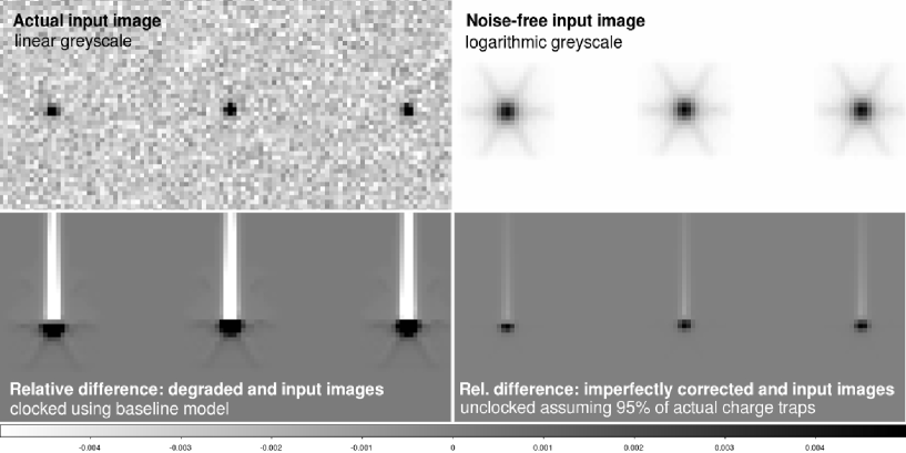
Charge Transfer Inefficiency has the greatest impact on small, faint objects that are far from the readout register (i.e. that have undergone a great number of transfers). To quantify the worst case scenario, we therefore simulate the smallest, faintest galaxy whose properties are likely to be measured – with an exponential flux profile $f(r)\propto\mathrm{e}^{-r}$ whose broad wings (compared to a Gaussian or de Vaucouleurs profile) also make it more susceptible to CTI. To beat down shot noise, we simulate $10^{7}$ noisy image realisations for each measurement. We locate these galaxies $2048\pm 0.5$ pixels from both the serial readout register and the amplifier, uniformly randomising the sub-pixel centre to average out effects that depend on proximity to a pixel boundary. All our simulated galaxies have the same circularly symmetric profile, following the observation by Rhodes et al. (2010) that this produces the same mean result as randomly oriented elliptical galaxies with no preferred direction.

We create the simulated images spatially oversampled by a factor 20, convolve them with a similarly oversampled Point Spread Function (PSF), then resample them to the final pixel scale. We use a preliminary PSF model and the $0\aas@@fstack{\prime\prime}1$ pixels of the Euclid VIS instrument, but our setup can easily be adapted to other instruments, e.g. ACS. To the image signal of $\sim\!\!1300$ electrons, we add a uniform sky background of $105$ electrons, as expected for a $560\,$s VIS exposure, and Poisson photon noise to both the source and the background. After clocking and charge trailing (if it is being done; see Sect. 4.1), we then add additional readout noise, which follows a Gaussian distribution with a root mean square (rms) of $4.5$ electrons, the nominal Euclid VIS value.

In the absence of charge trailing, the final galaxies have mean $S/N$=$11.35$, and Full Width at Half Maximum (FWHM) size of $0\aas@@fstack{\prime\prime}18$, as measured by SExtractor (Bertin & Arnouts 1996). This size, the same as the PSF, at the small end of the range expected from Fig. 4 of Massey et al. (2013) makes our galaxies the most challenging in terms of CTI correction. Examples of input, degraded, and corrected images are shown in Fig. 1.

Separately, we perform a second suite of simulations, containing $10^{6}$ realisations of a Euclid VIS PSF at $S/N\!\approx\!200$. The PSF simulations follow the above recipe, but skip the convolution of the PSF with an exponential disk.

2.2 Image analysis

On each of the sets of images (input, degraded, and corrected), we detect the sources using SExtractor. Moments of the brightness distribution and fluxes of the detected objects are measured using an IDL implementation of the RRG (Rhodes, Refregier & Groth 2001) shape measurement method. RRG is more robust than SExtractor for faint images, combining Gaussian-weighted moments of the image $I(\mn@boldsymbol{\theta})$ to measure integrated source flux

$$F\equiv\!\int{W(\mn@boldsymbol{\theta})\,I(\mn@boldsymbol{\theta})\,\mathrm{d}^{2}\mn@boldsymbol{\theta}},$$ (1)

where $W(\mn@boldsymbol{\theta})$ is a Gaussian weight function with standard deviation $w$, and the integral extends over $2.5w$; the position

$$y\equiv\!\int{\theta_{2}\,W(\mn@boldsymbol{\theta})\,I(\mn@boldsymbol{\theta})\,\mathrm{d}^{2}\mn@boldsymbol{\theta}};$$ (2)

the size

$$R^{2}\equiv Q_{11}+Q_{22};$$ (3)

and the ellipticity

$$\{e_{1},e_{2}\}\equiv\left\{\frac{Q_{11}-Q_{22}}{Q_{11}+Q_{22}},\frac{2Q_{12}}{Q_{11}+Q_{22}}\right\},$$ (4)

where the second-order brightness moments are

$$Q_{\alpha\beta}\!=\!\int{\theta_{\alpha}\,\theta_{\beta}\,W(\mn@boldsymbol{\theta})\,I(\mn@boldsymbol{\theta})\,\mathrm{d}^{2}\mn@boldsymbol{\theta}},\qquad\{\alpha,\beta\}\!\in\!\{1,2\}.$$ (5)

For measurements on stars, we chose a window size $w\!=\!0\aas@@fstack{\prime\prime}75$, the Euclid prescription for stars. For galaxies, we seek to reproduce the window functions used in weak lensing surveys. We adopt the radius of the SExtractor object (e.g. Leauthaud et al. 2007) that with $w\!=\!0\aas@@fstack{\prime\prime}34$ truncates more of the noise and thus returns more robust measurements.

Note that we are measuring a raw galaxy ellipticity, a proxy for the (reduced) shear, in which we are actually interested (cf. Kitching et al. 2012, for a recent overview of the effects a cosmic shear measurement pipeline needs to address). A full shear measurement pipeline must also correct ellipticity for convolution by the telescope’s PSF and calibrate it via a shear ‘responsivity factor’ (Kaiser, Squires & Broadhurst 1995). The first operation typically enlarges $e$ by a factor of $\sim 1.6$ and the second lowers it by about the same amount. Since this is already within the precision of other concerns, we shall ignore both conversions The absolute calibration of shear measurement with RRG may not be sufficiently accurate to be used on future surveys. However, it certainly has sufficient relative accuracy to measure small deviations in galaxy ellipticity when an image is perturbed.

3 High precision ellipticity measurements

3.1 Measurements of a non-linear quantity

A fundamental difficulty arises in our attempt to measure galaxy shapes to a very high precision, by averaging over a large number of images. Mathematically, the problem is that calculating ellipticity $e_{1}$ directly from the moments and then taking the expectation value $\mathcal{E}(\cdot)$ of all objects, i.e.:

$$e_{1}=\mathcal{E}\!\left(\frac{Q_{11}-Q_{22}}{Q_{11}+Q_{22}}\right),\quad e_{2}=\mathcal{E}\!\left(\frac{2Q_{12}}{Q_{11}+Q_{22}}\right),$$ (6)

means dividing one noisy quantity by another noisy quantity. Furthermore, the numerator and denominator are highly correlated. If the noise in each follows a Gaussian distribution, and their expectation values are zero, the probability density function of the ratio is a Lorentzian (also known as Cauchy) distribution. If the expectation values of the Gaussians are nonzero, as we expect, the ratio distribution becomes a generalised Lorentzian, called the Marsaglia-Tin distribution (Marsaglia 1965, 2006; Tin 1965). In either case, the ratio distribution has infinite second and first moments, i.e. its variance – and even its expectation value – are undefined. Implications of this for shear measurement are discussed in detail by Melchior & Viola (2012); Refregier et al. (2012); Kacprzak et al. (2012); Miller et al. (2013); Viola, Kitching & Joachimi (2014).

Therefore, we cannot simply average over ellipticity measurements for $10^{7}$ simulated images. The mean estimator (Eq. 6) would not converge, but follow a random walk in which entries from the broad wings of the distribution pull the average up or down by an arbitrarily large amount.

3.2 “Delta method” (Taylor expansion) estimators for ellipticity

As an alternative estimator, we employ what is called in statistics the ‘delta method’: a Taylor expansion of Eq. (6) around the expectation value of the denominator (e.g. Casella & Berger 2002). The expectation value of the ratio of two random variables $X$, $Y$ is thus approximated by:

$$\mathcal{E}(X/Y)\!\approx\!\frac{\mathcal{E}(X)}{\mathcal{E}(Y)}-\frac{\mathcal{C}(X,Y)}{\mathcal{E}^{2}(Y)}+\frac{\mathcal{E}(X)\sigma^{2}(Y)}{\mathcal{E}^{3}(Y)}\\ +\frac{\mathcal{C}(X,Y^{2})}{\mathcal{E}^{3}(Y)}-\frac{\mathcal{E}(X)\mathcal{E}[Y-\mathcal{E}(Y)]^{3}}{\mathcal{E}^{4}(Y)}$$ (7)

where $\mathcal{E}(X)$, $\sigma(X)$, $\sigma^{2}(X)$ denote the expectation value, standard deviation, and variance of $X$, and $\mathcal{C}(X,Y)$ its covariance with $Y$. The zero-order term in Eq. (7) is the often-used approximation $\mathcal{E}(X/Y)\approx\mathcal{E}(X)/\mathcal{E}(Y)$ that switches the ratio of the averages for the average of the ratio. We note that beginning from the first order there are two terms per order with opposite signs. Inserting Eq. (5) into Eq. (7), the first-order estimator for the ellipticity reads in terms of the brightness distribution moments $Q_{\alpha\beta}$ as follows:

$$\begin{split}e_{1}=&\frac{\mathcal{E}(Q_{11}\!-\!Q_{22})}{\mathcal{E}(Q_{11}\!+\!Q_{22})}\\ &-\frac{\sigma^{2}(Q_{11})\!-\!\sigma^{2}(Q_{22})}{\mathcal{E}^{2}(Q_{11}\!+\!Q_{22})}+\frac{\mathcal{E}(Q_{11}\!-\!Q_{22})\sigma^{2}(Q_{11}\!+\!Q_{22})}{\mathcal{E}^{3}(Q_{11}\!+\!Q_{22})}\end{split}$$ (8)

$$\begin{split}e_{2}=&\frac{\mathcal{E}(2Q_{12})}{\mathcal{E}(Q_{11}\!+\!Q_{22})}\\ &-\frac{\mathcal{C}(Q_{11},Q_{12})\!+\!\mathcal{C}(Q_{12},Q_{22})}{\mathcal{E}^{2}(Q_{11}\!+\!Q_{22})}+\frac{\mathcal{E}(2Q_{12})\sigma^{2}(Q_{11}\!+\!Q_{22})}{\mathcal{E}^{3}(Q_{11}\!+\!Q_{22})},\end{split}$$ (9)

with the corresponding uncertainties, likewise derived using the delta method (e.g. Casella & Berger 2002):

$$\begin{split}\sigma^{2}(e_{1})=&\frac{\sigma^{2}(Q_{11}\!-\!Q_{22})}{\mathcal{E}^{2}(Q_{11}\!+\!Q_{22})}\\ &-\frac{\mathcal{E}(Q_{11}\!-\!Q_{22})\left[\sigma^{2}(Q_{11})\!-\!\sigma^{2}(Q_{22})\right]}{\mathcal{E}^{3}(Q_{11}\!+\!Q_{22})}\\ &+\frac{\mathcal{E}^{2}(Q_{11}\!-\!Q_{22})\sigma^{2}(Q_{11}\!+\!Q_{22})}{\mathcal{E}^{4}(Q_{11}\!+\!Q_{22})}\end{split}$$ (10)

$$\begin{split}\sigma^{2}(e_{2})=&\frac{\sigma^{2}(Q_{11}\!+\!Q_{22})}{\mathcal{E}^{2}(Q_{11}\!+\!Q_{22})}\\ &-\frac{\mathcal{E}(Q_{11}\!+\!Q_{22})\left[\mathcal{C}(Q_{11},Q_{12})\!+\!\mathcal{C}(Q_{12},Q_{22})\right]}{\mathcal{E}^{3}(Q_{11}\!+\!Q_{22})}\\ &+\frac{\mathcal{E}^{2}(Q_{11}\!+\!Q_{22})\sigma^{2}(Q_{11}\!+\!Q_{22})}{\mathcal{E}^{4}(Q_{11}\!+\!Q_{22})}\quad.\end{split}$$ (11)

3.3 Application to our simulations

For our input galaxies, the combined effect of the first-order terms in eq. (8) is $\sim\!10$ %. Second-order contributions to the estimator are small, so we truncate after the first order. However, because of the divergent moments of the Marsaglia-Tin distribution, the third and higher-order contributions to the Taylor series increase again.

Nevertheless, while this delta-method estimator neither mitigates noise bias nor overcomes the infinite moments of the Marsaglia-Tin distribution at a fundamental level, it sufficiently suppresses the random walk behaviour for the purposes of this study, the averaging over noise realisations of the same object. We advocate re-casting the Euclid requirements in terms of the Stokes parameters ($Q_{11}\pm Q_{22},2Q_{12}$; Viola, Kitching & Joachimi 2014). These are the numerators and denominator of eq. (6) and are well-behaved Gaussians with finite first and second moments.

The formal uncertainties on ellipticity we quote in the rest of this article are the standard errors $\sigma(e_{1})/\sqrt{N}$ given by eq. (10). Our experimental setup of re-using the same simulated sources (computationally expensive due to the large numbers needed), our measurements will be intrinsically correlated (Sect. 4.2). Hence the error bars we show overestimate the true uncertainties.

4 The effects of fast and slow traps

4.1 How CTI is simulated

The input images are degraded using a C implementation of the Massey et al. (2014) CTI model. During each pixel-to-pixel transfer, in a cloud of $n_{\mathrm{e}}$ electrons, the number captured is

$$n_{\mathrm{c}}(n_{\mathrm{e}})=\left(1-\exp{\left(-\alpha n_{\mathrm{e}}^{1\!-\!\beta}\right)}\right)\sum_{i}\rho_{i}\left(\frac{n_{\mathrm{e}}}{w}\right)^{\beta},$$ (12)

where the sum is over different charge trap species with density $\rho_{i}$ per pixel, and $w$ is the full-well capacity. Parameter $\alpha$ controls the speed at which electrons are captured by traps within the physical volume of the charge cloud, which grows in a way determined by parameter $\beta$ .

Release of electrons from charge traps is modelled by a simple exponential decay, with a fraction $1-\mathrm{e}^{(-1/\tau_{i})}$ escaping during each subsequent transfer. The characteristic release timescale $\tau_{i}$ depends on the physical nature of the trap species and the operating temperature of the CCD.

In this paper, we make the simplifying ‘volume-driven’ assumption that charge capture is instantaneous, so $\alpha\!\!=\!\!0$. Based on laboratory studies of an irradiated VIS CCD (detailed in Sect. A), we adopt a $\beta\!=\!0.58$ baseline well fill, and end-of-life total density of one trap per pixel, $\rho\!=\!1$. In our first, general tests, we investigate a single trap species and explore the consequences of different values of $\tau$.

4.2 Iterative CTI correction

Figure 2: The effect on measurements of galaxy flux $F$, astrometry $y$ and morphology (size $R^{2}$, ellipticity $e_{1}$) of charge traps of different species, i.e. release timescale $\tau$. The pixel-to-pixel transfer is assumed to be instantaneous. Filled (open) circles denote data for faint galaxies before (after) CTI mitigation. Crosses (plus signs) denote data for bright stars before (after) CTI mitigation. Data for CTI-corrected images are shown multiplied by a factor of $10$ for $\Delta y$ and $\Delta e_{1}$. Lines give the best fit following Eq. (14), with the coefficients listed in Table LABEL:tab:taufits.

Table 1: Parameters of fitting functions to illustrate the effect on measurements of galaxy fluxes $F$ and $F_{\mathrm{S}}$, astrometry $y$ and morphology $R^{2}$, $e_{1}$ of charge traps of different species. In all cases, the measurements assume a density of one trap per pixel, and the astrophysical measurement is fitted as a function of the charge trap’s characteristic release time $\tau$ as $A+D_{a}\,{\mathrm{atan}}{((\log{\tau}-D_{p})/D_{w})}+G_{a}\exp{((\log{\tau}-G_{p})^{2}/2G_{w}^{2})}$. Values after correction highlight the efficacy of CTI mitigation.

	$A$	$D_{\mathrm{a}}$	$D_{\mathrm{p}}$	$D_{\mathrm{w}}$	$G_{\mathrm{a}}$	$G_{\mathrm{p}}$	$G_{\mathrm{w}}$
Galaxy simulation: in degraded images, including readout noise $\qquad[10\times$parameter]
$\Delta F/F_{\mathrm{true}}$	$-0.5367\pm 0.0098$	$-0.3144\pm 0.0085$	$6.199\pm 0.044$	$4.639\pm 0.260$	$0.2116\pm 0.0194$	$49.53\pm 1.64$	$41.54\pm 2.39$
$\Delta y$	$1.1098\pm 0.0014$	$-0.5291\pm 0.0028$	$8.392\pm 0.080$	$2.110\pm 0.234$	$0.3061\pm 0.0185$	$6.935\pm 0.402$	$7.083\pm 0.210$
$\Delta R^{2}/R^{2}_{\mathrm{true}}$	$0.4226\pm 0.0025$	$-0.3857\pm 0.0038$	$15.72\pm 0.18$	$2.576\pm 0.375$	$1.0866\pm 0.0448$	$4.382\pm 0.047$	$3.779\pm 0.160$
$\Delta e_{1}$	$0.5333\pm 0.0016$	$-0.3357\pm 0.0026$	$16.28\pm 0.22$	$2.951\pm 0.326$	$0.9901\pm 0.0203$	$4.553\pm 0.054$	$4.132\pm 0.081$
Galaxy simulation: after correction in software post-processing (perfect knowledge of charge traps) $\qquad[100\times$parameter]
$\Delta F/F_{\mathrm{true}}$	$-0.5549\pm 0.0029$	$0.0446\pm 0.0028$	$129.6\pm 13.7$	$26.00\pm 13.36$	$0.1301\pm 0.0121$	$73.47\pm 6.78$	$56.84\pm 5.21$
$\Delta y$	$0.09582\pm 0.01011$	$0.0517\pm 0.0111$	$5.622\pm 8.911$	$2.227\pm 4.557$	$0.0810\pm 0.1170$	$2.757\pm 5.369$	$3.154\pm 2.784$
$\Delta R^{2}/R^{2}_{\mathrm{true}}$	$-2.3181\pm 0.0173$	$0.4431\pm 0.0202$	$75.90\pm 25.02$	$28.47\pm 11.03$	$0.5471\pm 0.2294$	$41.31\pm 16.09$	$35.33\pm 9.12$
$\Delta e_{1}$	$0.01383\pm 0.0115$	$0.0039\pm 0.0066$	$12.30\pm 20.49$	$1.000\pm 0.000$	$0.0982\pm 0.0274$	$5.738\pm 2.085$	$5.353\pm 2.078$
Star simulation: in degraded images, including readout noise $\qquad[100\times$parameter]
$\Delta F/F_{\mathrm{true}}$	$-2.2472\pm 0.0239$	$-1.4558\pm 0.0189$	$107.5\pm 0.3$	$55.11\pm 0.95$	$1.151\pm 0.047$	$496.6\pm 3.2$	$343.6\pm 4.4$
$\Delta y$	$4.3532\pm 0.0014$	$-1.8608\pm 0.0027$	$173.1\pm 0.4$	$29.20\pm 0.67$	$5.0987\pm 0.0173$	$67.20\pm 0.20$	$43.91\pm 0.22$
$\Delta R^{2}/R^{2}_{\mathrm{true}}$	$0.9489\pm 0.00098$	$-6.434\pm 0.0095$	$288.8\pm 4.7$	$18.71\pm 4.49$	$20.237\pm 0.716$	$94.42\pm 0.15$	$50.20\pm 0.25$
$\Delta e_{1}$	$1.2336\pm 0.0077$	$-0.7941\pm 0.0086$	$266.7\pm 2.4$	$17.54\pm 3.90$	$16.513\pm 0.046$	$94.87\pm 0.19$	$52.57\pm 0.21$
Star simulation: after correction in software post-processing (perfect knowledge of charge traps) $\qquad[100\times$parameter]
$\Delta F/F_{\mathrm{true}}$	$-0.0035\pm 0.0002$	$0.0027\pm 0.0003$	$110.2\pm 10.5$	$42.21\pm 20.02$	$0.0006\pm 0.0271$	$182.6\pm 71.3$	$3.5\pm 100.0$
$\Delta y$	$0.1504\pm 0.00066$	$0.0970\pm 0.0067$	$12.46\pm 1.86$	$2.731\pm 1.552$	$0.0218\pm 0.0034$	$7.377\pm 1.024$	$5.063\pm 0.717$
$\Delta R^{2}/R^{2}_{\mathrm{true}}$	$-0.0163\pm 0.0038$	$-0.0182\pm 0.0036$	$1269\pm 33$	$24.57\pm 47.63$	$0.0198\pm 0.0146$	$50.83\pm 34.56$	$37.95\pm 38.64$
$\Delta e_{1}$	$0.0012\pm 0.0024$	$0.0003\pm 0.0014$	$2.26\pm 50.92$	$1.000\pm 0.000$	$0.02668\pm 0.0061$	$8.465\pm 1.800$	$5.379\pm 1.647$

The Massey et al. (2014) code can also be used to ‘untrail’ the CTI. If required, we use $n_{\mathrm{iter}}=5$ iterations to attempt to correct the image (possibly with slightly different model parameters). Note that we perform this correction only after adding readout noise in the simulated images.

Our main interest in this study is the impact of uncertainties in the trap model on the recovered estimate of an observable $\eta$ (e.g. ellipticity). Therefore, we present our results in terms of differences between the estimators measured for the corrected images, and the input values:

$$\Delta\eta_{i}=\eta_{i,\mathrm{corrected}}-\eta_{i,\mathrm{input}}.$$ (13)

Because for each object of index $i$ the noise in the measurements of $\eta_{i,\mathrm{corrected}}$ and $\eta_{i,\mathrm{input}}$ are strongly correlated, they partially cancel out. Thus the actual uncertainty of each $\Delta\eta_{i}$ is lower than quoted. Moreover, because we re-use the same noise realisation in all our measurements (cases of different $\rho_{i}$ and $\tau_{i}$), these measurements are correlated as well.

4.3 CTI as a function of trap timescale

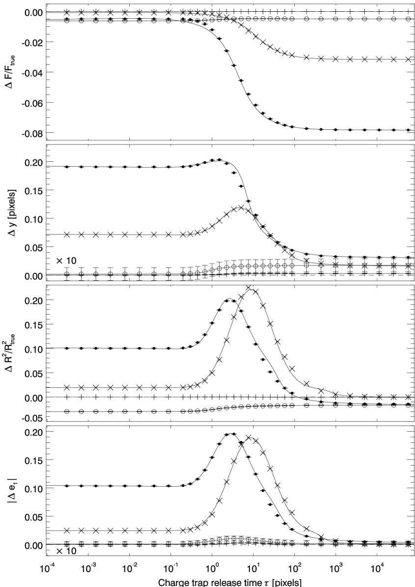
The impact of charge trapping is dependent on the defect responsible. Figure 2 demonstrates the effect of charge trap species with different release times $\tau$ on various scientific observables. To compute each datum (filled symbols), we simulate $10^{7}$ galaxies, add shot noise, add CTI trailing in the $y$ direction (i.e. vertical in Fig. 1), only then add readout noise. Separately, we simulate $10^{6}$ stars. Using eqs. (8)–(11), we measure mean values of photometry (top panel), astrometry (second panel) and morphology (size in the third, and ellipticity in the bottom panel). Our results confirm what Rhodes et al. (2010) found in a different context.

Three trap regimes are apparent, for all observables. Very fast traps ($\tau\!\la\!0.3$ transfers) do not displace electrons far from the object; thus their effect on photometry is minimal (top plot in Fig. 2). We observe significant relative changes in position, size, and ellipticity, forming a plateau at low $\tau$, because even if captured electrons are released after the shortest amount of time, some of them will be counted one pixel off their origin. This is probably an artifact: We expect the effect of traps with $\tau\!<\!0.1$ to be different in an model simulating the transfer between the constituent electrodes of the physical pixels, rather than entire pixels.

Very slow traps ($\tau\!\ga\!30$ transfers) result in electrons being carried away over a long distance such that they can no longer be assigned to their original source image. Hence, they cause a charge loss compared to the CTI-free case. However, because charge is removed from nearly everywhere in the image, their impact on astrometry and morphology is small.

The most interesting behaviour is seen in the transitional region, for traps with a characteristic release time of a few transfer times. If electrons re-emerge several pixels from their origin, they are close enough to be still associated with their source image, but yield the strongest distortions in size and ellipticity measurements. This produces local maxima in the lower two panels of Fig. 2. If these measurements are scientifically important, performance can – to some degree – be optimised by adjusting a CCD’s clock speed or operating temperature to move release times outside the most critical range $1\!\la\!\tau\!\la\!10$ (Murray et al. 2012).

In the star simulations (crosses in Fig. 2 for degraded images, plus signs for CTI-corrected images), the CTI effects are generally smaller than for the faint galaxies, because the stars we simulate are brighter and thus experience less trailing relative to their signal. Still, we measure about the same spurious ellipticity $\Delta e_{1}$ and even a slightly higher relative size bias $\Delta R^{2}/R^{2}_{\mathrm{true}}$ for the stars. The explanation is that the quadratic terms in the second-order moments (eq. 5) allow for larger contributions from the outskirts of the object, given the right circumstances. In particular, the wider window size $w$ explains the differences between the galaxy and PSF simulations. Notably, the peak in the $\Delta e_{1}(\tau)$ and $\Delta R^{2}/R^{2}_{\mathrm{true}}(\tau)$ curves shifts from $\sim\!3\,\mbox{px}$ for the galaxies to $\sim\!9\,\mbox{px}$ for the stars. Because the wider window function gives more weight to pixels away from the centroid, the photometry becomes more sensitive to slower traps.

For a limited number of trap configurations, we have also tried varying the trap density or the number of transfers (i.e. object position on the CCD). In both cases, the dependence is linear. Overall, for all tested observables, the measurements in the degraded images (Fig. 2, solid symbols) are well-fit by the empirical fitting function

$$f^{\mathrm{degrade}}(\rho,\tau)=\rho\Big{(}A+D_{\mathrm{a}}\,{\mathrm{atan}}{((\log{\tau}-D_{\mathrm{p}})/D_{\mathrm{w}})}+\\ G_{\mathrm{a}}\exp{((\log{\tau}-G_{\mathrm{p}})^{2}/2G_{\mathrm{w}}^{2})}\Big{)},$$ (14)

which combines an arc-tangent drop (“D”) and a Gaussian peak (“G”). The best fit-amplitudes ($A$, $D_{\mathrm{a}}$ and $G_{\mathrm{a}}$), positions on the $\tau$ axis ($D_{\mathrm{p}}$ and $G_{\mathrm{p}}$) and widths ($D_{\mathrm{w}}$ and $G_{\mathrm{w}}$), are listed in Table LABEL:tab:taufits. The same functional form provides a good match to the residuals after CTI correction, $f^{\mathrm{resid}}(\rho,\tau)$ (open symbols in Fig. 2). These residuals are caused by readout noise, which is not subject to CTI trailing, but undergoes CTI correction (see Sect. 5.3.2).

4.4 Predictive model for imperfect correction

We set out to construct a predictive model $\Delta f^{\mathrm{Pr}}$ of $\Delta\eta$, the CTI effect in an observable relative to the underlying true value (eq. 13). There are two terms, the CTI degradation (eq. 14), and a second term for the effect of the ‘inverse’ CTI correction allowing for a slightly imperfect CTI model:

$$\Delta f^{\mathrm{Pr}}=f^{\mathrm{degr}}(\rho,\tau)+f^{\mathrm{correct}}(\rho+\Delta\rho,\tau+\Delta\tau).$$ (15)

Since CTI trailing perturbs an image by only a small amount, the correction acts on an almost identical image. Assuming the coefficients of eq. (14) to be constant, we get:

$$\Delta f^{\mathrm{Pr}}\approx f^{\mathrm{degr}}(\rho,\tau)-f^{\mathrm{degr}}(\rho+\Delta\rho,\tau+\Delta\tau)+f^{\mathrm{res}}(\rho,\tau),$$ (16)

where $f^{\mathrm{res}}(\rho,\tau)$ is approximately constant, and depends on the readout noise (see Section 5.3). We could expand this equation as a Taylor series, but the derivatives of $f$ do not provide much further insight.

Because eq. (12) is non-linear in the number $n_{\mathrm{e}}$ of signal electrons, our observation (Sect. 4.3) that the effects of CTI behave linearly in $\rho$ is not a trivial result. Assuming this linearly in $\rho$, we can expand eq. (16) and factor out $\rho$. The combined effect of several trap species $i$ with release timescales $\tau_{i}$ and densities $\rho_{i}$ can then be written as:

$$\Delta f^{\mathrm{Pr}}(\rho_{i}+\Delta\rho_{i},\tau_{i}+\Delta\tau_{i})\!=\!\sum_{i}\rho_{i}f^{\mathrm{resid}}(\tau_{i})+\\ \sum_{i}\left[\rho_{i}f(\tau_{i})-(\rho_{i}+\Delta\rho_{i})f(\tau_{i}+\Delta\tau_{i})\right],$$ (17)

in which we dropped the superscript of $f^{\mathrm{degr}}$ for the sake of legibility. We are going to test this model in the remainder of this study, where we consider a mixture of three trap species. We find eq. (17) to correctly describe measurements of spurious ellipticity $\Delta e_{1}$, as well as the relative bias in source size $\Delta R^{2}/R^{2}_{\mathrm{true}}$ and flux $\Delta F/F_{\mathrm{true}}$.

5 Euclid as a concrete example

5.1 Context for this study

To test the general prediction eq. (17), we now evaluate the effect of imperfect CTI correction in simulations of Euclid data, with a full Euclid CTI model featuring multiple trap species (see Sect. 5.2). We call this the $\mathbf{M}+\delta\mathbf{M}$ experiment.

Akin to Prod’homme et al. (2012) for Gaia, this study is useful in the larger context of the flow down of requirements from Euclid’s science goals (Refregier et al. 2010) to its imaging capabilities (Massey et al. 2013) and instrument implementation (Cropper et al. 2013, 2014). In particular, Massey et al. (2013) highlight that the mission’s overall success will be determined both by its absolute instrumental performance and our knowledge about it. We now present the next step in the flow down: to what accuracy do we need to constrain the parameters of the Massey et al. (2014) CTI model? Future work will then determine which calibration observations are required to achieve this accuracy.

While the final Euclid requirements remain to be confirmed, we adopt the current values as discussed by Cropper et al. (2013). Foremost, the “CTI contribution to the PSF ellipticity shall be $<\!1.1\times 10^{-4}$ per ellipticity component”.

The Euclid VIS PSF model will bear an uncertainty due to CTI, that translates into an additional error on measured galaxy properties. For the bright stars (which have much higher $S/N$) tracing the PSF, Cropper et al. (2013) quote a required knowledge of $R^{2}$ to a precision $\left|\sigma(R^{2})\right|\!<\!4\times 10^{-4}$. We test this requirement with our second suite of simulations, containing $10^{6}$ realisations of a Euclid VIS PSF at $S/N\!\approx\!200$ (cf. Sec. 2.1).

In reality, CTI affects the charge transport in both CCD directions, serial and parallel. For the sake of simplicity, we only consider serial CTI, and thus underestimate the total charge trailing. There is no explicit photometric error budget allocated to CTI, while “ground data processing shall correct for the detection chain response to better than $0.7$ % error in photometry in the nominal VIS science images”.

5.2 CTI model for the Euclid VISual instrument

Table 2: The baseline trap model $\mathcal{M}$. The model includes a baseline well fill power of $\beta_{0}\!=\!0.58$.

Baseline model	$i\!=\!1$	$i\!=\!2$	$i\!=\!3$
Trap density $\rho_{i}$ [px-1]	$0.02$	$0.03$	$0.95$
Release timescale $\tau_{i}$ [px]	$0.8$	$3.5$	$20.0$

Figure 3: Residual spurious ellipticity and source size induced by CTI after correction, as a function of the rms readout noise. Left plot: Spurious ellipticity $\Delta e_{1}$ in the faintest galaxies to be analysed for Euclid, at the end of the mission, and furthest from the readout register. Right plot: Bias in source size $\Delta R^{2}/R^{2}_{\mathrm{true}}$ in bright stars, at the end of the mission, and furthest from the readout register. Lines show the best quadratic (cubic) fits. Shaded regions indicate the Euclid VIS requirements. Vertical grey lines mark the nominal rms readout noise of $4.5$ electrons.

Based on a suite of laboratory test data, we define a baseline model $\mathbf{M}$ of the most important CTI parameters ($\rho_{i}$, $\tau_{i}$, $\beta_{0}$). We degrade our set of $10^{7}$ simulated galaxies using $\mathbf{M}$. The $\mathbf{M}+\delta\mathbf{M}$ experiment then consists of correcting the trailing in the degraded images with slight alterations to $\mathbf{M}$. We investigate $>\!100$ correction models $\mathbf{M}+\delta\mathbf{M}$, resulting in an impressive $1.4\times 10^{9}$ simulated galaxies used in this study.

Exposure to the radiation environment in space was simulated in the laboratory by irradiating a prototype of the e2v CCD273 to be used for Euclid VIS with a $10$ MeV equivalent fluence of $4.8\!\times\!10^{9}\,\mathrm{protons/cm}^{-2}$ (Prod’homme et al. 2014; Verhoeve et al. 2014). Characterisation experiments were performed in nominal VIS conditions of $153\,\mbox{K}$ temperature and a $70\,\mbox{kHz}$ readout frequency. We refer to Appendix A for further details on the experiments and data analysis.

We emphasize that our results for $e_{1}$ pertain to faint and small galaxies, with an exponential disk profile (vz. Sect. 2.1), and placed at the maximum distance from the readout register ($y\!=\!2051$ transfers). Furthermore, we assume the level of radiation damage expected at the end of Euclid’s six year mission. Because CTI trailing increases roughly linearly with time in orbit (cf. Massey et al. 2014), the CTI experienced by the typical faintest galaxy (i.e. at half the maximum distance to the readout register and three years into the mission), will be smaller by a factor of $4$ compared to the results quoted below.

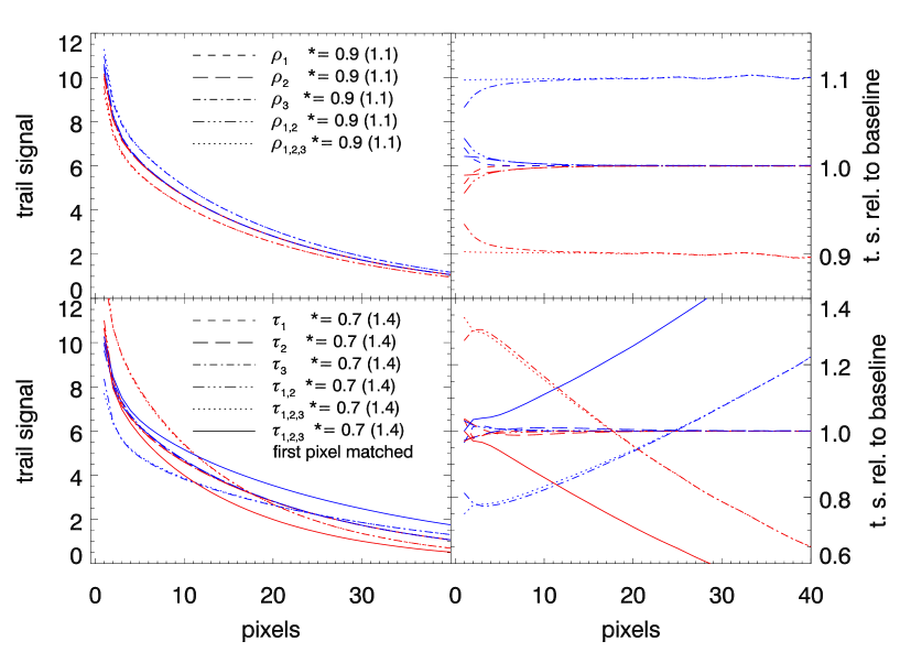
Where not stated otherwise the nominal Euclid VIS rms readout noise of $4.5$ electrons was used. Table LABEL:tab:traps summarises the baseline model $\mathbf{M}$ that was constructed based on these analyses. The default well fill power is $\beta_{0}\!=\!0.58$. Slow traps with $\tau_{3}\!=\!20$ clock cycles and $\rho_{3}\!=\!0.95$ dominate our baseline model, with small fractions of medium-fast ($\tau_{2}\!=\!3.5$, $\rho_{2}\!=\!0.03$) and fast ($\tau_{1}\!=\!0.8$, $\rho_{1}\!=\!0.02$) traps. Figure 12 shows how trails change with changing trap parameters.

5.3 Readout noise impedes perfect CTI correction

5.3.1 Not quite there yet: the zeropoint

First, we consider the ellipticities measured in the degraded and corrected images, applying the same baseline model in the degradation and correction steps. The reasons why this experiment does not retrieve the same corrected ellipticity $e_{\mathrm{corr}}$ as input ellipticity $e_{\mathrm{in}}$ are the Poissonian image noise and Gaussian readout noise. We quantify this in terms of spurious ellipticity $\Delta e\!=\!e_{\mathrm{corr}}-e_{\mathrm{in}}$, and shall refer to it as the zeropoint of the $\mathbf{M}+\delta\mathbf{M}$ experiment. The spurious ellipticity in the serial direction is $Z_{\mathrm{e_{1}}}\!=\!\Delta e_{1}\!=\!-0.00118\pm 0.00060$. Thus, this experiment on worst-case galaxies using the current software exceeds the Euclid requirement of $\left|\Delta e_{\alpha}\right|\!<\!1.1\times 10^{-4}$ by a factor of $\sim\!10$. With respect to the degraded image $99.68$ % of the CTI-induced ellipticity are being corrected. Virtually the same zeropoint, $\Delta e_{1}\!=\!-0.00118\pm 0.00058$, is predicted by adding the contributions of the three species from single-species runs based on the full $10^{7}$ galaxies. We point out that these results on the faintest galaxies furthest from the readout register have been obtained using non-flight readout electronics (cf. Short et al. 2014).

From our simulation of $10^{6}$ bright ($S/N\!\approx\!200$) stars, we measure the residual bias in source size $R^{2}$ after CTI correction of $Z_{\!R^{2}}\!=\!\Delta R^{2}/R^{2}_{\mathrm{true}}\!=\!(-0.00112\pm 0.00030)$, in moderate excess of the requirement $\left|\Delta R^{2}/R^{2}_{\mathrm{true}}\right|\!<\!4\times 10^{-4}$. While the $S/N$ of the star simulations is selected to represent the typical Euclid VIS PSF tracers, the same arguments of longest distance from the readout register and non-flight status of the electronics apply.

5.3.2 The effect of readout noise

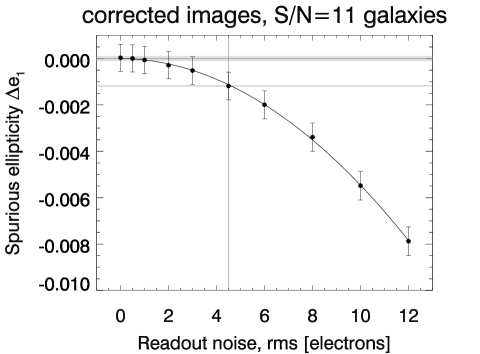
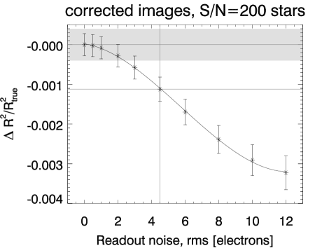
In Fig. 3, we explore the effect of varying the rms readout noise in our simulations about the nominal value of $4.5$ electrons (grey lines) discussed in Sect. 5.3.1. We continue to use the baseline trap model for both degradation and correction. For the rms readout noise, a range of values between $0$ and $15$ electrons was assumed. For the faint galaxies (Fig. 3, left plot), we find $\Delta e_{1}$ to increase with readout noise in a way well described by a second-order polynomial. A similar, cubic fit can be found for $\Delta R^{2}/R^{2}_{\mathrm{true}}$ measured from the star simulations (Fig. 3, right plot), but with a hint towards saturation in the highest tested readout noise level.

The most important result from Fig. 3 is that in absence of readout noise, if the correction assumes the correct trap model $\mathbf{M}$, it removes the CTI perfectly, with $\Delta e_{1}\!=\!(0.3\pm 5.9)\times 10^{-4}$ and $\Delta R^{2}/R^{2}_{\mathrm{true}}\!=\!(0.0\pm 2.8)\times 10^{-4}$. The quoted uncertainties are determined by the $N\!=\!10^{7}$ ($10^{6}$) galaxy images we simulated. We conclude that the combination of our simulations and correction code pass this crucial sanity check. If the rms readout noise is $\lesssim\!3$ electrons ($\lesssim\!0.5$ electrons), the spurious ellipticity (the relative size bias) stays within Euclid requirements.

5.4 Sensitivity to imperfect CTI modelling

5.4.1 Morphology biases as a function of well fill power, and determining tolerance ranges

Figure 4: Sensitivity of the CTI-induced spurious ellipticity $\Delta e_{1}$ (upper plot) and the relative spurious source size $\Delta R^{2}/R^{2}_{\mathrm{true}}$ (lower plot) to the well fill power $\beta$. At the default value of $\beta\!=\!0.58$ (vertical grey line), the measurements deviate from zero due to readout noise, as indicated by arrows. The shaded region around the measurements indicate the Euclid requirement ranges as a visual aid. Solid and dashed lines display quadratic (linear) fits to the measured $\Delta e_{1}(\beta)$ and $\Delta R^{2}(\beta)/R^{2}_{\mathrm{true}}$, respectively. We study the worst affected objects (at the end of the mission and furthest from the readout register) and the faintest Euclid galaxies. This plot also assumes CTI is calibrated from charge injection lines at full well capacity only. This will not be the case.

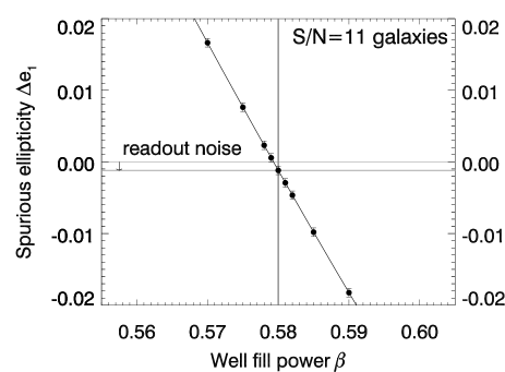
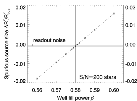
Now that we have assessed the performance of the correction using the same CTI model as for the degradation (given the specifications of our simulations), we turn to the $\mathbf{M}+\delta\mathbf{M}$ experiment for determining the sensitivities to imperfections in the CTI model. To this end, we assume the zeropoint offset $Z_{e_{1}}$ (or $Z_{\!R^{2}}$) of Sect. 5.3.1 to be corrected, and ‘shift’ the requirement range to be centred on it (see, e.g., Fig. 4).

Figure 4 shows the $\mathbf{M}+\delta\mathbf{M}$ experiment for the well fill power $\beta$. If the degraded images are corrected with the baseline $\beta_{0}\!=\!0.58$, we retrieve the zeropoint measurement from Sect. 5.3.1. For the $\mathbf{M}+\delta\mathbf{M}$ experiment, we corrected the degraded images with slightly different well fill powers $0.56\!\leq\!\beta\!\leq\!0.60$. The upper plot in Fig. 4 shows the resulting $\Delta e_{1}$ in galaxies, and the lower plot $\Delta R^{2}/R^{2}_{\mathrm{true}}$ in stars. We find a strong dependence of both the spurious serial ellipticity $\Delta e_{1}$ and $\Delta R^{2}/R^{2}_{\mathrm{true}}$ on $\Delta\beta\!=\!\beta\!-\!\beta_{0}$.

In order to determine a tolerance range with respect to a CTI model parameter $\xi$ with baseline value $\xi_{0}$ (here, the well fill power $\beta$), we fit the measured bias $\Delta\eta$ (e.g. $\Delta e_{1}$, cf. eq. 13) as a function of $\Delta\xi\!=\!\xi\!-\!\xi_{0}$. By assuming a polynomial

$$\Delta\eta(\Delta\xi)=Z_{\eta}+\sum_{j=1}^{J}{a_{j}(\Delta\xi)^{j}}$$ (18)

of low order $J$, we perform a Taylor expansion around $\xi_{0}$. In eq. 18, $Z_{\eta}$ is the zeropoint (Sect. 5.3.1) to which we have shifted our requirement margin. The coefficients $a_{j}$ are determined using the IDL singular value decomposition least-square fitting routine SVDFIT. For consistency, our fits include $Z_{\eta}$ as the zeroth order. In Fig. 4, the best-fitting quadratic (linear) fits to $\Delta e_{1}$ ($\Delta R^{2}/R^{2}_{\mathrm{true}}$) are shown as a solid and dashed line, respectively.

In both plots, the data stick tightly to the best-fitting lines, given the measurement uncertainties. If the measurements were uncorrelated, this would be a suspiciously orderly trend. However, as already pointed out in Sect. 3.3, we re-use the same $10^{7}$ simulations with the same peaks and troughs in the noise in all data points shown in Figs. 4 to 9. Hence, we do not expect to see data points to deviate from the regression lines to the degree their quoted uncertainties would indicate. As a consequence, we do not make use of the $\chi^{2}_{\mathrm{red}}\!\ll\!1$ our fits commonly yield for any interpretation.

Because the interpretation of the reduced $\chi^{2}$ is tainted by the correlation between our data points, we use an alternative criterion to decide the degree $J$ of the polynomial: If the uncertainty returned by SVDFIT allows for a coefficient $a_{j}\!=\!0$, we do not consider this or higher terms. For the panels of Fig. 4, this procedure yields $J\!=\!2$ ($J\!=\!1$). The different signs of the slopes are expected because $R^{2}$ appears in the denominator of eq. (4).

Given a requirement $\Delta\eta_{\mathrm{req}}$, e.g. $\Delta e_{1,\mathrm{req}}\!=\!1.1\times 10^{-4}$, the parametric form (eq. 18) of the sensitivity curves allows us to derive tolerance ranges to changes in the trap parameters. Assuming the zeropoint (the bias at the correct value of $\xi$) to be accounted for, we find the limits of the tolerance range as the solutions $\Delta\xi_{\mathrm{tol}}$ of

$$\left|\sum_{j=1}^{J}{a_{j}(\Delta\xi)^{j}}\right|\!=\!\Delta\eta_{\mathrm{req}}$$ (19)

with the smallest values of $|\Delta\xi|$ on either sides to $\Delta\xi\!=\!0$. Using, eq. (19), we obtain $\Delta\beta_{\mathrm{tol}}\!=\!\pm(6.31\pm 0.07)\times 10^{-5}$ from the requirement on the spurious ellipticity $\Delta e_{1}\!<\!1.1\times 10^{-4}$, for which the quadratic term is small. From the requirement on the relative size bias $\Delta R^{2}/R^{2}_{\mathrm{true}}\!<\!4\!\times\!10^{-4}$ we obtain $\Delta\beta_{\mathrm{tol}}\!=\!\pm(4.78\pm 0.05)\times 10^{-4}$. In other words, the ellipticity sets the more stringent requirement, and we need to be able to constrain $\beta$ to an accuracy of at least $(6.31\pm 0.07)\times 10^{-5}$ in absolute terms. This analysis assumes calibration by a single charge injection line at full well capacity, such that eq. (12) needs to be extrapolated to lower signal levels. We acknowledge that Euclid planning has already adopted using also faint charge injection lines, lessening the need to extrapolate.

5.4.2 Ellipticity bias as a function of trap density

Figure 5: Sensitivity of the CTI-induced spurious ellipticity $\Delta e_{1}$ in faint galaxies (upper panel) and relative bias in source size $\Delta R^{2}/R^{2}_{\mathrm{true}}$ (lower panel) in bright stars to a relative change in trap densities $(\rho_{i}+\Delta\rho_{i})/\rho_{i}$. Different symbols and line styles denote which to which of the trap species a change in density was applied: The slow traps: ($\rho_{1}$, upward and dashed line); the medium traps: ($\rho_{2}$, downward triangles and long-dashed line); both of them: ($\rho_{1}$, $\rho_{2}$, diamonds and triple dot-dashed line); the fast traps ($\rho_{3}$, squares and dot-dashed line); all: ($\rho_{1}$, $\rho_{2}$, $\rho_{3}$, circles and dotted line). The various broken lines show the best-fit representation of the measurements as given by the sensitivity model (Eq. 20). Like in Fig. 4, the grey shaded area indicates the Euclid VIS requirement range. We study the worst affected objects (at the end of the mission and furthest from the readout register) and the faintest Euclid galaxies.

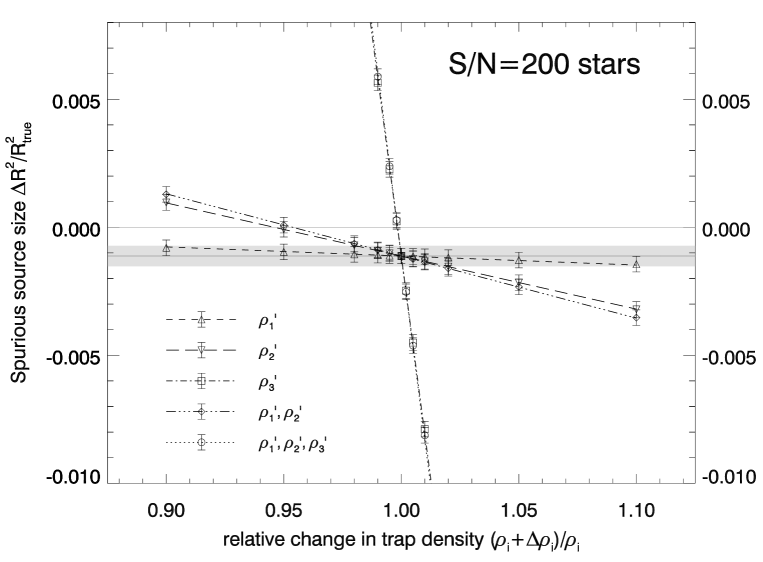
We now analyse the sensitivity of $\Delta e_{\alpha}$ towards changes in the trap densities. Figure 5 shows the $\mathbf{M}+\delta\mathbf{M}$ experiment for one or more of the trap densities $\rho_{i}$ of the baseline model. The upper panel of Fig. 5 presents the spurious ellipticity $\Delta e_{1}$ for five different branches of the experiment. In each of the branches, we modify the densities $\rho_{i}$ of one or several of the trap species. For example, the upward triangles in Fig. 5 denote that the correction model applied to the images degraded with the baseline model used a density of the fast trap species $\rho_{1}\!+\!\Delta\rho_{1}$, tested at several values of $\Delta\rho_{1}$ with $0.9\!\leq\!1\!+\!\Delta\rho_{1}/\rho_{1}\!\leq\!1.1$. The densities of the other species are kept to their baseline values in this case. The other four branches modify $\rho_{2}$ (downward triangles); $\rho_{3}$ (squares); $\rho_{1}$ and $\rho_{2}$ (diamonds); and all three trap species (circles).

Because a value of $\Delta\rho_{i}\!\!=\!\!0$ reproduces the baseline model in all branches, all of them recover the zeropoint measurement of $\Delta e_{1}$ there (cf. Sect. 5.3.1). Noticing that $e_{\mathrm{degr,1}}\!-\!e_{\mathrm{in,1}}\!<\!0$ for the degraded images relative to the input images, we explain the more negative $\Delta e_{1}$ for $\Delta\rho_{i}\!<\!0$ as the effect of undercorrecting the CTI. This applies to all branches of the experiment. Likewise, with increasing $\Delta\rho_{i}\!>\!0$, the residual undercorrection at the zeropoint decreases. Eventually, with even higher $\kappa\!>\!1$, we overcorrect the CTI and measure $\Delta e_{1}\!>\!0$.

Over the range of $0.9\!\leq\!1\!+\!\Delta\rho_{1}/\rho_{1}\!\leq\!1.1$ we tested, $\Delta e_{1}$ responds linearly to a change in the densities. Indeed, our model (eq. 17), which is linear in the $\rho_{i}$ and additive in the effects of the different trap species, provides an excellent description of the measured data, both for $\Delta e_{1}$ and $\Delta R^{2}/R^{2}_{\mathrm{true}}$ (Fig. 5, lower panel). The lines in Fig. 5 denote the model prediction from a simplified version of eq. (17),

$$\Delta f^{\mathrm{Pr}}(\rho_{i}+\Delta\rho_{i})\!=\!\sum_{i}\rho_{i}f^{\mathrm{resid}}(\tau_{i})+\sum_{i}(\rho_{i}+\Delta\rho_{i})f(\tau_{i})\,.$$ (20)

In eq. (20), we assumed the $\tau_{i}$ be correct, i.e. $\Delta\tau_{i}\!=\!0$.

Next, we compute the tolerance $\Delta\rho_{i,\mathrm{tol}}/\rho$ by which, for each branch of the experiment, we might deviate from the correct trap model and still recover the zeropoint within the Euclid requirements of $\left|\Delta e_{\alpha,\mathrm{req}}\right|\!<\!1.1\times 10^{-4}$, resp.  $\left|\Delta R^{2}_{\mathrm{req}}/R^{2}_{\mathrm{true}}\right|\!<\!4\times 10^{-4}$. Again, we calculate these tolerances about the zeropoints $Z\!=\!\sum_{i}\rho_{i}f^{\mathrm{resid}}(\tau_{i})$ (cf. eq. 20), that we found to exceed the requirements in Sect. 5.3.1, but assume to be corrected for in this experiment.

In accordance with the linearity in $\Delta\rho_{i}$, applying the Taylor expansion recipe of Sect. 5.4.1, we find the data in Fig. 5 to be well represented by first-order polynomials (eq. 18). The results for $\Delta\rho_{i,\mathrm{tol}}/\rho$ we obtain from eq. (19) are summarised in Table LABEL:tab:tolerances. For all species, the constraints from $\Delta e_{1}$ for faint galaxies are tighter than the ones from $\Delta R^{2}/\Delta R^{2}_{\mathrm{true}}$ for bright stars.

Only considering the fast traps, $\rho_{1}$ can change by $0.84\pm 0.33$% and still be within Euclid VIS requirements, given the measured zeropoint has been corrected for. While a tolerance of $0.39\pm 0.06$% is found for $\rho_{2}$, the slow traps put a much tighter tolerance of $0.0303\pm 0.0007$% on the density $\rho_{3}$. This is expected because slow traps amount to $95$% of all baseline model traps (Table LABEL:tab:traps). Varying the density of all trap species in unison, we measure a tolerance of $0.0272\pm 0.0005$%.

Computing the weighted mean of the $\Delta\tau\!=\!0$ intercepts in Fig. 5, we derive better constraints on the zeropoints: $Z_{\mathrm{e_{1}}}\!=\!\Delta e_{1}\!=\!-0.00117\pm 0.00008$ for the faint galaxies, and $Z_{\!R^{2}}\!=\!\Delta R^{2}/R^{2}_{\mathrm{true}}\!=\!-0.00112\pm 0.00004$ for the bright stars.

5.4.3 Ellipticity bias as a function of trap release time

Figure 6: Sensitivity of the CTI-induced spurious ellipticity $\Delta e_{1}$ in faint galaxies (upper panel) and relative bias in source size $\Delta R^{2}/R^{2}_{\mathrm{true}}$ (lower panel) in bright stars to a relative change in release timescales $(\tau_{i}+\Delta\tau_{i})/\tau_{i}$. Different symbols and line styles denote to which of the trap species a change in release timescale was applied: The slow traps: ($\tau_{1}$, upward triangles and dashed line); the medium traps: ($\tau_{2}$, downward triangles and long-dashed line); both of them: ($\tau_{1}$, $\tau_{2}$, diamonds and triple dot-dashed line); the fast traps ($\tau_{3}$, squares and dot-dashed line); all: ($\tau_{1}$, $\tau_{2}$, $\tau_{3}$, circles and dotted line). The various broken lines show the best-fit representation of the measurements as given by the empiric sensitivity model (eq. 21). Like in Fig. 4, the grey shaded area indicates the VIS Euclid requirement range. We study the worst affected objects (at the end of the mission and furthest from the readout register) and the faintest Euclid galaxies.

Table 3: Tolerances for changes in the trap model parameters $\xi$ (column 1), derived from polynomial fits to the sensitivity curves, and taking into account the Euclid VIS requirements (eqs. 18, 19). Here, we assume no residual biases when using the correct trap model. For three observables $\eta$, we show pairs of tolerances, for $\Delta\xi\!<\!0$ and $\Delta\xi\!>\!0$ each. Columns 2 and 3 report tolerances based on the ellipticity bias $\Delta e_{1}$, columns 4 and 5 those from the relative size bias $\Delta R^{2}/R^{2}_{\mathrm{true}}$, and columns 6 and 7 those from the relative flux bias $\Delta F/F_{\mathrm{true}}$.

branch $\xi$	$10^{4}\Delta\xi_{\mathrm{tol}}^{\mathrm{min}}$	$10^{4}\Delta\xi_{\mathrm{tol}}^{\mathrm{max}}$	$10^{4}\Delta\xi_{\mathrm{tol}}^{\mathrm{min}}$	$10^{4}\Delta\xi_{\mathrm{tol}}^{\mathrm{max}}$	$10^{4}\Delta\xi_{\mathrm{tol}}^{\mathrm{min}}$	$10^{4}\Delta\xi_{\mathrm{tol}}^{\mathrm{max}}$
	$\eta\!=\!\Delta e_{1}$	$\eta\!=\!\Delta e_{1}$	$\eta\!=\!\Delta R^{2}/R^{2}_{\mathrm{true}}$	$\eta\!=\!\Delta R^{2}/R^{2}_{\mathrm{true}}$	$\eta\!=\!\Delta F/F_{\mathrm{true}}$	$\eta\!=\!\Delta F/F_{\mathrm{true}}$
	galaxies	galaxies	stars	stars	galaxies	galaxies
$\beta$	$-0.631\pm 0.007$	$0.631\pm 0.007$	$-4.78\pm 0.05$	$4.78\pm 0.05$	$-61.5\pm 0.3$	$60.5\pm 0.3$
$\rho_{1}$	$-84_{-33}^{+18}$	$84_{-18}^{+33}$	$-1250_{-1800}^{+450}$	$1250_{-450}^{+1800}$	$--$	$--$
$\rho_{2}$	$-39_{-6}^{+4}$	$39_{-4}^{+6}$	$-191_{-19}^{+16}$	$191_{-16}^{+19}$	$--$	$--$
$\rho_{3}$	$-3.03_{-0.07}^{+0.06}$	$3.03_{-0.06}^{+0.07}$	$-5.91\pm 0.03$	$5.91\pm 0.03$	$-267.5\pm 1.6$	$267.5\pm 1.6$
$\rho_{1,2}$	$-26_{-3}^{+2}$	$26_{-2}^{+3}$	$-166_{-14}^{+12}$	$166_{-12}^{+14}$	$--$	$--$
$\rho_{1,2,3}$	$-2.72\pm 0.05$	$2.72\pm 0.05$	$-5.71\pm 0.03$	$5.71\pm 0.03$	$-262.8\pm 1.6$	$262.8\pm 1.6$
$\tau_{1}$	$-193_{-23}^{+19}$	$193_{-19}^{+23}$	$-1310_{-150}^{+120}$	$1310_{-120}^{+150}$	$<-10000$	$>10000$
$\tau_{2}$	$-300_{-360}^{+90}$	$270_{-70}^{+150}$	$-270_{-70}^{+50}$	$270_{-50}^{+80}$	$<-10000$	$>10000$
$\tau_{3}$	$-4.00\pm 0.04$	$4.00\pm 0.04$	$-11.30\pm 0.05$	$11.31\pm 0.05$	$-1574_{-23}^{+24}$	$2320_{-90}^{+100}$
$\tau_{1,2}$	$-420_{-420}^{+150}$	$700_{-400}^{+900}$	$-220_{-50}^{+30}$	$230_{-40}^{+50}$	$<-10000$	$>10000$
$\tau_{1,2,3}$	$-4.03\pm 0.04$	$4.04\pm 0.04$	$-11.69\pm 0.05$	$11.68\pm 0.05$	$-1454_{-20}^{+19}$	$2020_{-60}^{+70}$
$\tau_{1,2,3},\rho_{1,2,3}$, first pixel matched	$-16.07_{-0.61}^{+0.57}$	$16.09_{-0.57}^{+0.61}$	$-16.17\pm 0.09$	$16.21\pm 0.09$	$-262.5\pm 0.7$	$263.0\pm 0.7$

Figure 6 shows the $\mathbf{M}+\delta\mathbf{M}$ experiment for one or more of the release timescales $\tau_{i}$ of the trap model. The upper panel of Fig. 6 presents the spurious ellipticity $\Delta e_{1}$ for five different branches of the experiment. In each of the branches, we modify the release timescales $\tau_{i}$ of one or several of the trap species by multiplying it with a factor $(\tau_{i}+\Delta\tau_{i})/\tau_{i}$.

As in Fig. 5, the upward triangles in Fig. 6 denote that the correction model applied to the images degraded with the baseline model used a density of $\tau_{1}+\Delta\tau_{1}$ for the fast trap species. The release timescales of the other species are kept to their baseline values in this case. The other four branches modify $\tau_{2}$ (downward triangles); $\tau_{3}$ (squares); $\tau_{1}$ and $\tau_{2}$ (diamonds); and all three trap species (circles).

Because a value of $\Delta\tau\!=\!0$ reproduces the baseline model in all branches, all of them recover the zeropoint measurement of $\Delta e_{1}$ there. The three trap species differ in how the $\Delta e_{1}$ they induce varies as a function of $\Delta\tau_{i}$. One the one hand, for $\tau_{1}$, we observe more negative $\Delta e_{1}$ for $(\tau_{i}+\Delta\tau_{i})/\tau_{i}\!<\!1$ , and less negative values for $(\tau_{i}+\Delta\tau_{i})/\tau_{i}\!>\!1$, with a null at $(\tau_{i}+\Delta\tau_{i})/\tau_{i}\!\approx\!1.5$. On the other hand, with the slow traps ($\tau_{3}$), we find $\Delta e_{1}\!>\!0$ for $(\tau_{i}+\Delta\tau_{i})/\tau_{i}\!\la\!0.99$, and more negative values than the zeropoint for $(\tau_{i}+\Delta\tau_{i})/\tau_{i}\!>\!1$. The curve of $\Delta e_{1}(\lambda\tau_{2})$ shows a maximum at $(\tau_{i}+\Delta\tau_{i})/\tau_{i}\!\approx\!0.8$, with a weak dependence on $0.7\!\la\!(\tau_{i}+\Delta\tau_{i})/\tau_{i}\!\la\!1.1$.

Key to understanding the spurious ellipticity as a function of the $\tau_{i}$ is the dependence of $\Delta e_{1}(\tau)$ for a single trap species that we presented in Fig. 2, and expressed by the empirical fitting function $f_{\mathrm{e_{\alpha}}}(\tau)$ (Eq. 14) with the parameters quoted in Table LABEL:tab:tolerances. While the correction algorithm effectively removes the trailing when the true $\tau_{i}$ is used, the residual of the correction will depend on the difference between the $\Delta e_{\alpha}$ for $\tau_{i}$ and for the timescale $(\tau_{i}+\Delta\tau_{i})/\tau_{i}$ actually used in the correction. This dependence is captured by the predictive model (Eq. 17), which simplifies for the situation in Fig. 6 ($\Delta\rho_{i}\!=\!0$) to

$$\Delta f^{\mathrm{Pr}}(\tau_{i}+\Delta\tau_{i})\!=\!Z+\sum_{i}\rho_{i}\left[f(\tau_{i})-f(\tau_{i}+\Delta\tau_{i})\right],$$ (21)

with $Z\!=\!\sum_{i}\rho_{i}f^{\mathrm{resid}}(\tau_{i})$ (lines in Fig. 6). In the branches modifying $\tau_{1}$ and/or $\tau_{2}$, but not $\tau_{3}$, the measurements over the whole range of $0.5\!\leq\!(\tau_{i}+\Delta\tau_{i})/\tau_{i}\!\leq\!1.6$ agree with the empirical model within their uncertainties. If $\tau_{3}$ is varied, Eq. (21) overestimates $|\Delta e_{1}|$ significantly for $|\Delta\tau_{i}|\!>\!0.05\tau_{i}$. We discuss a possible explanation in Sect. 6. Our empirical model provides a natural explanation for the maximum in $\Delta e_{1}(\tau_{2})$: Because $\tau_{2}\!=\!3.5$ is located near the peak in $f_{\mathrm{e_{1}}}(\tau)$, assuming $(\tau_{i}+\Delta\tau_{i})/\tau_{i}\!\leq\!0.8$ for correction means using a release time regime where $\Delta e_{1}(\tau)$ is still rising instead of falling. The correction software accounts for this; hence the spurious ellipticity from using the wrong release time scale shows the same maximum as $f_{\mathrm{e_{1}}}(\tau)$.

Because $\tau_{2}$ is not located very closely to the peak in $\Delta R^{2}/\Delta R^{2}_{\mathrm{true}}(\tau)$ (cf. Fig. 2), we do not see an extremum in the lower panel of Fig. 6 which shows the sensitivity of the size bias in bright stars to variations in the $\tau_{i}$.

In order to compute the tolerances $\Delta\tau_{\mathrm{tol}}$ towards changes in the release timescales, we again employ a polynomial fit (eq. 19). Evidently, the tolerances differ substantially between the $\tau_{i}$, again with the narrower tolerance intervals from $\Delta e_{1}$ than from $\Delta R^{2}/\Delta R^{2}_{\mathrm{true}}$. Only for $\Delta\tau_{2}$ with its extreme point for $\Delta e_{1}$ near the baseline value, we find similar tolerances in both cases. However, even for the rare trap species $\tau_{1}$, the tolerance is only $\Delta\tau_{1,\mathrm{tol}}\!=\!(1.93\pm 0.23)$ %. One needs to know the release timescale of the slow trap species to an accuracy of $(0.0400\pm 0.0004)$ % to be able to correct it within Euclid VIS requirements. We find the same tolerance if all timescales are varied in unison.

5.4.4 Combinations of timescales and densities yielding the same first trail pixel flux

Figure 7: The same as Fig. 6, but for $\Delta\tau_{i}\!<\!0$ combinations of timescales $\tau_{i}$ and densities $\rho_{i}$ that yield the same count rate in the first trail pixel as the baseline model. All trap species are modified in unison (large symbols and solid line). For comparison, small symbols and the dotted line repeat the result from Fig. 6, where only the $\tau_{i}$ were modified, not the $\rho_{i}$. (Notice the different scale of the ordinates.) The lines show the predictive models (Eq. 17). We study the worst affected objects (end of the mission, furthest from the readout register) and the faintest Euclid galaxies.

Considering how trap parameters are constrained practically from Extended Pixel Edge Response (EPER) and First Pixel Response (FPR) data, it is instructive to consider combinations of trap release timescales $\tau_{i}$ and densities $\rho_{i}$ that yield the same number of electrons in the first pixel of the trail as the baseline model. This is interesting because given realistic conditions, the first pixel of the trail will have the largest signal-to-noise ratio and will be most easily constrained. We thus perform an initial exploration of the parameter degeneracies. In our “first pixel matched” models, the effect of a given change in $\tau$ on the first trail pixel needs to be compensated by a change in $\rho$. Because a larger (smaller) $\tau$ means more (less) charge close to the original pixel, the compensation requires $\Delta\rho_{i}\!<\!0$ for $\Delta\tau_{i}\!<\!1$ and $\Delta\rho_{i}\!>\!1$ for $\Delta\tau_{i}\!>\!1$. Only in the branches where we vary $\tau_{3}$ or all timescales together, we find the $\Delta\rho_{i}$ to differ noticeably from unity. For the latter two, they populate a range between $\Delta\rho_{i}\!=\!0.745$ for $\Delta\tau_{i}\!=\!0.7$ to $\Delta\rho_{i}\!=\!1.333$ for $\Delta\tau\!=\!1.4$.

Figure 7 shows the $\mathbf{M}+\delta\mathbf{M}$ experiment for all $\tau_{i}$ and $\rho_{i}$ (large symbols). Small symbols depict the alteration to $\tau_{i}$, but with the $\rho_{i}$ kept fixed, i.e. the same measurement as the open circles in Fig. 6. Compared to these, $\Delta e_{1}$ in faint galaxies (upper panel) is of opposite sign in the “first pixel matched” case, relative to the zeropoint. This can be understood as an effect of our baseline trap mix being dominated by slow traps, for which a small increase in $\tau$ leads to less CTI-induced ellipticity. The simultaneous increase in trap density effects more CTI-induced ellipticity, and this is the larger of the two terms, such that a change in sign ensues. The same holds for $\Delta R^{2}/R^{2}_{\mathrm{true}}$ in bright stars (lower panel of Fig. 7), but with inverted slopes compared to $\Delta e_{1}$.

Again using eq. (19), we compute the tolerance range for the changes to the $\tau_{i}$ in the “first pixel matched” case. (The respective changes to the $\rho_{i}$ are determined by the first pixel constraint.) Modifying all release time scales, we arrive at $\Delta\tau_{\mathrm{tol}}\!=\!0.16$ %. (Table LABEL:tab:tolerances). This tolerance is wider than the $0.04$% for $\Delta e_{1}$ when only the $\tau_{i}$ are varied, again due to the different signs arising from variations to $\tau_{3}$ and $\rho_{3}$. By coincidence, we also arrive at $\Delta\tau_{\mathrm{tol}}\!=\!0.16$ % when repeating that test with the size bias measured in bright stars.

The black solid line in Fig. 7 shows the predictive model (eq. 17), taking into account the combined effect of the $\Delta\tau_{i}$ and $\Delta\rho_{i}$, giving the same first pixel flux. Both in the $\tau_{i}$-only (dotted line) and “first pixel matched” cases it matches the measurements only within a few percent from $\lambda\!=\!1$. Crucially, this mismatch only occurs for $\Delta e_{1}$ in faint galaxies, but not for $\Delta R^{2}/R^{2}_{\mathrm{true}}$ in bright stars.

We explain this discrepancy with the uncertainties with which our measurements and modelling (Fig. 2) describe the underlying function $f_{\mathrm{e_{1}}}(\tau)$. The range $20\!\la\!\tau\!\la\!100$ is where the fitting function Eq. (14) deviates most from the observations in Fig. 2. The CTI correction effectively removes almost all CTI effects on photometry and morphology, leaving the residuals presented in Figs. 5 to 9, at least one order of magnitude smaller than the scales of the uncorrected CTI effects. Hence, a relatively small uncertainty in $f(\tau)$ causes a large mismatch with the data.

The cause of the uncertainty in the parameters of Eq. (14), shown in Table LABEL:tab:taufits, is twofold: First, there is uncertainty in the fit as such. Second, there is uncertainty due to the finite sampling of the $\Delta e_{\alpha}(\tau)$ and $\Delta F_{\mathrm{rel}}(\tau)$ curves. Running a denser grid in $\tau$ can remove the latter, but the former might be ultimately limited by our choice of the function (Eq. 14), which is empirically motivated, not physically. We further discuss the limits of the predictive model in Sect. 6.

5.5 Residual flux errors after imperfect CTI correction

5.5.1 Flux bias as a function of readout noise

Figure 8: Relative bias in RRG flux with respect to the true input flux, as a function of readout noise (upper panel) and well fill power $\beta$ (lower panel). Solid lines give the best-fit polynomial models. The grey-shaded Euclid requirement range is centred on zero for the readout noise plot, and on the zeropoint corresponding to the default readout noise for the $\beta$ plot. Measurement uncertainties are shown, but very small. We study the worst affected objects (end of the mission, furthest from the readout register) and the faintest Euclid galaxies.

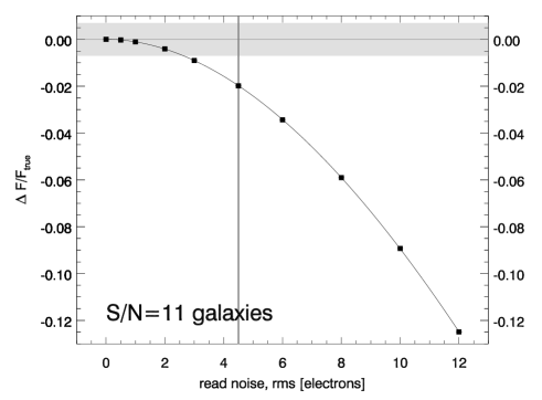
Given the default rms readout noise of $4.5$ electrons, we measure a flux bias $\Delta F_{\mathrm{rel}}\!=\!\Delta F/F_{\mathrm{true}}$ relative to the true flux $F_{\mathrm{true}}$ in the input faint galaxy simulations of $(-1.980\pm 0.012)$ % after CTI correction, corresponding to $92.9$ % of the CTI-induced flux bias being corrected. The upper panel of Fig. 8 shows the relative flux biases before and after correction as a function of rms readout noise. Without readout noise, the flux bias can be corrected perfectly ($\Delta F_{\mathrm{rel}}\!=\!(0.002\pm 0.012)\times 10^{-2}$ after correction). With increasing readout noise, the flux bias deteriorates, in a way that can be fitted with a cubic polynomial in terms of readout noise. Comparing to the degraded images, we notice that the correction software applies same amount of correction, independent of the readout noise. Because the mitigation algorithm in its current form does not include a readout noise model, this confirms our expectations.

We show the Euclid requirement on photometric accuracy as the grey-shaded area in Fig. 8 (upper panel), centred on zero. The nominal readout noise case exceeds the requirement of $<\!0.7$ % photometric uncertainty for the faintest, worst-affected galaxies we study. However, the CTI-induced bias affects all VIS images, and would thus be calibrated out. The Euclid flux requirement can be understood as pertaining to uncertainties, not biases in the photometric calibration. The uncertainty of the flux bias, $0.0012$ % then makes only a tiny contribution to the photometric error budget. We now go on to study the sensitivity of the flux bias towards changes in the trap model.

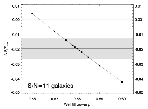
5.5.2 Flux bias as a function of well fill power $\beta$

The lower panel of Fig. 8 shows how a change in well fill power $\beta$ alters the flux bias. If we correct the degraded images using a $\beta\!>\!\beta_{0}$, the model accounts for less CTI in small charge packages, i.e. less CTI in the image’s wings that are crucial for both photometry and morphology (cf. fig. 4) Hence, a $\beta\!>\!\beta_{0}$ leads to an undercorrection relative to the flux bias zeropoint $Z_{\mathrm{F}}$ (Sect. 5.5.1), while for $\beta\!-\!\beta_{0}\!\la\!-0.017$, the zero line is crossed and overcorrection occurs.

Although $\Delta F_{\mathrm{rel}}(\beta)$ in Fig. 8 appears linear, using the criterion based on significant components (Sect. 5.4.2), a quadratic is preferred, indicated by the solid line. Using eq. (19), we compute the tolerance range in $\beta$ given $\Delta F_{\mathrm{rel}}(\beta_{\mathrm{tol}})\!=\!0.007$, centred on $Z_{\mathrm{F}}$. Towards smaller well fill powers, we find $\Delta\beta_{\mathrm{tol}}^{\mathrm{min}}\!=\!-(6.15\pm 0.03)\times 10^{-3}$, while towards larger $\beta$, we find $\Delta\beta_{\mathrm{tol}}^{\mathrm{max}}\!=\!(6.05\pm 0.03)\times 10^{-3}$. Compared to the constraints on the knowledge of $\beta$ from $\Delta e_{1}$ derived in Sect. 5.4.1, these margins are $\sim\!100$ times wider.

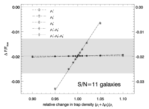
5.5.3 Flux bias as a function of trap densities

The upper plot of Fig. 9 shows the flux bias $\Delta F_{\mathrm{rel}}$ in dependence of a change $\Delta\rho_{i}$ to the densities $\rho_{i}$ in the correction model, in analogy to Sect. 5.4.2. Unless the density of the dominant trap species $\rho_{3}$ is modified, we measure only insignificant departures from the zeropoint $Z_{\mathrm{F}}$. Given the high accuracy of the flux measurements, these are still significant measurements, but they are negligible with respect to the Euclid requirement on flux. If all $\rho_{i}$ are varied in unison, the effect on $\Delta F_{\mathrm{rel}}$ is largest. A linear model using Eq. (18) yields a tolerance of $\Delta\rho_{i}^{\mathrm{tol}}/\rho_{i}\!=\!\pm 2.628\pm 0.016$ %, wider than the tolerances for $\Delta e_{1}$ or $\Delta R^{2}/R^{2}_{\mathrm{true}}$ (Table LABEL:tab:tolerances). The lines in the upper plot of Fig. 9 show that the model (eq. 20) matches our measurements well over the range in $\Delta\rho_{i}$ we tested.

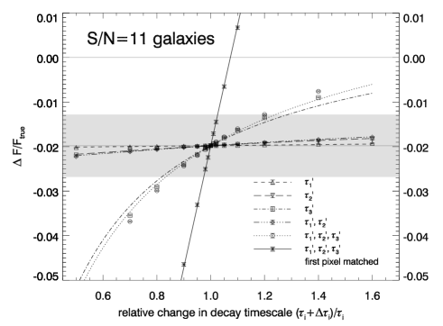
5.5.4 Flux bias as a function of release timescales

The lower plot of Fig. 9 shows the flux bias $\Delta F_{\mathrm{rel}}$ in dependence of a change $\Delta\tau_{i}$ in the correction model, like in Sect. 5.4.3. As for varying the $\rho_{i}$ (Sect. 5.5.3), a change to only the fast and/or the medium traps yields only small departures from the zeropoint such that we can bundle together all trap species for deriving a tolerance range. The respective measurements (black circles in Fig. 9) show a steep slope at $\Delta\tau_{i}\!<\!0$ that flattens out to $\Delta\tau_{i}\!>\!0$. This can be explained given the saturation of $\Delta F_{\mathrm{rel}}$ found at large $\tau$ in Fig. 2 and is confirmed by our model (eq. 21; dotted line in Fig. 9). Our prediction is offset from the measurement due to uncertainties in the modelling, but the slopes agree well.

Although polynomial fits using eq. (18) warrant cubic terms in both cases, $\Delta F_{\mathrm{rel}}(\tau_{i}\!+\!\Delta\tau_{i})$ is much straighter in the “first pixel matched” case where also the $\rho_{i}$ are altered (star symbols in Fig. 9; cf. Sect. 5.4.4). The reason is that the slopes of $\Delta F_{\mathrm{rel}}(\rho_{i}\!+\!\Delta\rho_{i})$ and $\Delta F_{\mathrm{rel}}(\tau_{i}\!+\!\Delta\tau_{i})$ have the same sign and do not partially cancel each other out, as is the case for $\Delta e_{1}(\rho_{i}\!+\!\Delta\rho_{i})$ and $\Delta e_{1}(\tau_{i}\!+\!\Delta\tau_{i})$. Again, eq. (17) succeeds in predicting the measurements, despite offsets that are significant given the small uncertainties but small in terms of $\Delta F_{\mathrm{rel}}$ in the uncorrected images.

Using the cubic fits, we find the following wide tolerance ranges (eq. 19) $\Delta\tau_{3,\mathrm{min}}^{\mathrm{tol}}/\tau_{3}\!=\!15.7\pm 0.2$ % and $\Delta\tau_{3,\mathrm{max}}^{\mathrm{tol}}/\tau_{3}\!=\!23.2_{-0.9}^{+1.0}$ %. In the “first pixel matched”, case the intervals are considerably tighter, due to the contribution from the change in densities, with $\Delta\tau_{i,\mathrm{min}}^{\mathrm{tol}}/\tau_{i}\!=\!2.625\pm 0.007$ % and $\Delta\tau_{i,\mathrm{max}}^{\mathrm{tol}}/\tau_{i}\!=\!2.630\pm 0.007$ %. Again, the strictest constraints come from the ellipticity component $\Delta e_{1}$.

Figure 9: Upper panel: The same as Fig. 5, but showing the sensitivity of the measured flux bias $\Delta F/F_{\mathrm{true}}$ as a function of the relative change in trap densities $\rho_{i}$. Lower panel: The same as Fig. 6, but showing the flux bias $\Delta F/F_{\mathrm{true}}$ as a function of the relative change in trap densities $\tau_{i}$. Star symbols and the solid line denote the “first pixel matched” model for all trap species. The lines in both panels show the predictive model (eq. 17). We study the worst affected objects (end of the mission, furthest from the readout register) and the faintest Euclid galaxies.

6 Discussion

6.1 Limits of the predictive model

We measured tolerance ranges for changes in the $\rho_{i}$ and $\tau_{i}$ given the Euclid VIS requirements, and presented a model (Eq. 17) capable of predicting these results based on the $\Delta\eta(\tau)$ curves (e.g. $\Delta e_{1}(\tau)$, Fig. 2), that are less expensive to obtain in terms of CPU time. However, as can be seen in particular in Fig. 7, there is a mismatch between predictions and measurements for $\tau_{3}$, the most common baseline model trap species. As discussed in Sect. 5.4.4, this is caused by the finite sampling and the empirical nature of eq. (14).

Unfortunately, $f(\tau)$ and $f^{\mathrm{resid}}(\tau)$ will likely depend non-trivially on the source profile. Moreover, Eq. (17), if applied to ellipticity, treats it as additive. Where this approximation breaks down, i.e. when values that are not $\ll\!1$ are involved, the correct additional formula (e.g. Schneider 2006) must be used. This applies to CTI-induced ellipticity as well as to large intrinsic or shear components.

We tested that the dependence on $\beta$ (Fig. 4) can be included in the model as well, yielding

$$\Delta f^{\mathrm{Pr}}(\beta,\rho_{i},\tau_{i})\!=\!\sum_{i}\rho_{i}f^{\mathrm{resid}}(\tau_{i})+[f(\beta\!+\!\Delta\beta)\!-\!f(\beta)]\\ \times\sum_{i}\left[\rho_{i}f(\tau_{i})-(\rho_{i}\!+\!\Delta\rho_{i})f(\tau_{i}\!+\!\Delta\tau_{i})\right].$$ (22)

6.2 Applicability

Our findings pertain specifically to CTI correction employing the Massey et al. (2014) iterative correction scheme, the current nominal procedure for Euclid VIS. Other algorithms for the removal of CTI trailing exist that might not be susceptible in the same way to readout noise. Prod’homme et al. (2012), investigating the full-forward approach designed for Gaia, did not observe a readout noise floor similar to the one we found. The same might hold for including CTI correction in a forward-modelling shear measurement pipeline (e.g. Miller et al. 2013). However, the Gaia method has not been applied yet to actual observational data, and the Massey et al. (2014) is the most accurate method for the CTI correction of real data today.

We remind the reader that our results on the zeropoints upon correcting with the correct model (Fig. 4) are dependent on the specifics of the small and faint galaxies we simulated. Further tests will determine if the large bias in $R^{2}$ persists under more realistic scenarios.

The narrow tolerances of $\Delta\rho/\rho\!=\!0.11$% and $\Delta\tau/\tau\!=\!0.17$% for the density of the slow traps species might look daunting, but fortunately, due to the discernible trails caused by these traps it is also the easiest species of which to determine the properties. Conversely, the $\Delta\rho/\rho\!=\!3$% and $\Delta\tau/\tau\!=\!8$% for the fast traps are much larger, but constraints on these traps will be harder to achieve from laboratory and in-flight calibration data. Considering the “first pixel matched” case, taking into account how trap parameters are determined from CTI trails, relaxes the tolerances from ellipticity but tightens the (much broader) tolerances from the photometric, for our particular baseline trap mix. We notice that, while trap parameters are degenerate and Sect. 5.4.4 marks a first attempt to disentangle these parameters, each (degenerate) set of parameters can yield a viable CTI correction. Characterising the true trap species, however, is crucial with respect to device physics applications.

Source profile-dependence of the CTI-induced flux bias $\Delta F_{\mathrm{rel}}$ will lead to a sample of realistic sources (i.e. with a distribution of source profiles) showing a range in $\Delta F_{\mathrm{rel}}$ at any given readout noise level. Thus, the uncertainty in $\Delta F_{\mathrm{rel}}$ will be larger than the $10^{-4}$ we measured for our broad-winged, but homogeneous images in Sect. 5.5.1. More sophisticated simulations are necessary to assess the role of the variable CTI-induced flux bias in Euclid’s photometric error budget.

7 Conclusions and Outlook

The goal was to bridge the divide between engineering measurements of CTI, and its degradation of scientific measurements of galaxy shapes. We have developed a very fast algorithm to model CTI in irradiated e2v Technologies CCD273 devices, reproducing laboratory measurements performed at ESTEC. We take a worst-case approach and simulate the faintest galaxies to be studied by Euclid, with a broad-winged exponential profile, at the end of the mission and furthest away from the readout register. Our analysis is hindered by the divergent surface brightness moments of the Marsaglia-Tin distribution that the ellipticity components follow. We alleviate this problem by means of a Taylor expansion around the mean of the denominator, yielding an accuracy of $\sigma e_{\alpha}\!\approx\!10^{-4}$ by averaging over $10^{7}$ simulated images. We advocate that Euclid requirements be re-defined in a way that avoids ratios of noisy quantities.

Our detailed study of the trapping process has confirmed that not all traps are equally bad for shape measurement (Rhodes et al. 2010): Traps with release timescales of a few clocking cycles cause the largest spurious ellipticity, while all traps with longer $\tau_{i}$ yield the strongest flux bias.

The impact of uncertainties in the trap densities $\rho_{i}$ and time scales $\tau_{i}$ on CTI effects can be predicted to a satisfactory accuracy by a model that is linear in the $\rho_{i}$ and additive in the effects of different trap species. For future applications, this will allow us to reduce the simulational effort in CTI forecasts, calculating the effect of trap pixels from single species data.

Informed by laboratory data of the irradiated CCD273, we have adopted a baseline trap model for Euclid VIS forecasts. We corrected images with a trap model $\mathbf{M}+\delta\mathbf{M}$ offset from the model $\mathbf{M}$ used for applying CTI. Thus we derived tolerance ranges for the uncertainties in the trap parameters, given Euclid requirements, positing that the required level of correction will be achieved. We conclude:

1.

In the absence of readout noise, perfect CTI correction in terms of ellipticity and flux can be achieved.

2.

Given the nominal rms readout noise of $4.5$ electrons, we measure $Z_{\mathrm{e_{1}}}\!=\!\Delta e_{1}\!=\!-1.18\times 10^{-3}$ after CTI correction. This still exceeds the Euclid requirement of $\left|\Delta e_{1}\right|\!<\!1.1\times 10^{-4}$. The requirement may still be met on the actual ensemble of galaxies Euclid will measure, since we consider only the smallest galaxies of $S/N\!=\!11$. Likewise, in $S/N\!=\!200$ stars, we measure a size bias of $1.12\times 10^{-3}$, exceeding the requirement of $\left|\Delta R^{2}/R^{2}_{\mathrm{true}}\right|\!<\!4\times 10^{-4}$.

3.

The spurious ellipticity $\Delta e_{1}$ sensitively depends on the correct well fill power $\beta$, which we need to constrain to an accuracy of $\Delta\beta_{\mathrm{tol}}\!=\!(6.31\pm 0.07)\times 10^{-5}$ to meet requirements. This assumes calibration by a single, bright charge injection line. The narrowest tolerance intervals are found for the dominant slow trap species in our baseline mix: $\Delta\rho_{\mathrm{tol}}/\rho_{0}\!=\!(\pm 0.0272\pm 0.0005)$%, and $\Delta\tau_{\mathrm{tol}}/\tau_{0}\!=\!(\pm 0.0400\pm 0.004)$%.

4.

Given the nominal rms readout noise, we measure a flux bias $Z_{\mathrm{F}}\!=\!\Delta F_{\mathrm{rel}}\!=\!(-1.980\pm 0.012)$% after CTI correction, within the required $\left|\Delta F_{\mathrm{rel}}\right|\!<\!0.7$ % for the photometric uncertainty. More relevant for Euclid will be the uncertainty of this bias, which for realistic sources depends on their source profile. Further study is necessary here, as well as for the impact of CTI on photometric nonlinearity.

The final correction will only be as good as on-orbit characterisation of physical parameters such as trap locations, density and release time. The next steps building on this study should include: 1.) Researching and testing novel algorithms mitigating the effects of read noise as part of the CTI correction. 2.) Characterising the effect of realistic source profile distributions in terms of the photometric and nonlinearity requirements. 3.) Translating the tolerances in trap model parameters into recommendations of calibration measurements and their analysis, based on modelling the characterisation of trap species.

Plans for Euclid VIS calibration have already been updated to include charge injection at multiple levels such that $\beta$ does not need to be extrapolated from bright charge injection lines to faint galaxies. We will continue to liaise between engineers and scientists to determine how accurately it will be necessary to measure these physical parameters. The VIS readout electronics will be capable of several new in-orbit calibration modes such as trap pumping (Murray et al. 2012) that are not possible with HST, and our calculations will advise what will be required, and how frequently they need to be performed, in order to adequately characterise the instrument for scientific success.

Appendix A Informing the baseline model with laboratory data

A.1 EPER/FPR data with irradiated CCD

Figure 10: CCD273 EPER trails in the serial (upper plot) and parallel (lower plot) directions. Shown here are the G quadrant trails at an input signal of $\sim\!1000$ electrons. Solid lines within the light and dark grey shaded areas denote the average and its uncertainty of the profile before and after correction for electronic effects. The best-fit model to the corrected trail is shown as a long-dashed line. For the purpose of illustration, the baseline trap model is shown in both plots as a short-dashed line. Building on the serial EPER model, the baseline model includes fast traps that are seen in quadrant F.

Figure 11: The well fill power $\beta$ measured from the integrated EPER CTI as a function of input signal. The upper panel shows the results from the serial EPER measurements, for which CTI is present in the F and G quadrants and can be corrected using the E and H quadrants. The lower panel shows the results from the parallel EPER measurements, for which CTI is present in the F, G, and H quadrants and can be corrected using the E quadrant. Open symbols denote the raw measurements, filled symbols the calibrated measurements from which the fits for $\beta$ are derived.

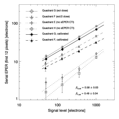
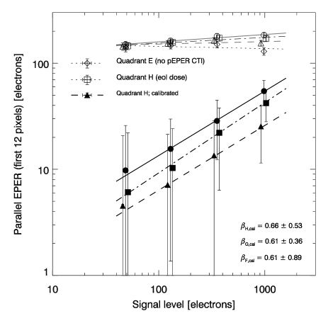
In this Appendix, we define a baseline CTI model for Euclid VIS. Our model is based upon laboratory tests of an irradiated e2v Technologies back-illuminated Euclid prototype CCD273, analysed at ESA/ESTEC (Prod’homme et al. 2014). The device was irradiated at ambient room temperature using $10.4$ MeV protons, degraded from a $38.5$ MeV primary proton beam at the Kernfysisch Versneller Instituut, Groningen, in April 2013. Two different shielding masks were used (Prod’homme et al. 2014) resulting in the four quadrants of the CCD, called E, F, G, and H, and corresponding to the four output nodes, receiving different radiation doses. Each a half of two quadrants, called G and H, received a $10$ MeV equivalent fluence of $4.8\times 10^{9}\,\mbox{protons}/\mbox{cm}^{-2}$, representative of the predicted end-of-life (eol) proton fluence for Euclid. Half of the F quadrant was irradiated with a $10$ MeV equivalent fluence of $2.4\times 10^{9}\,\mbox{protons}/\mbox{cm}^{-2}$, the $\mbox{eol}/2$ fluence. Neither the E quadrant, the serial register of the H quadrant, nor the readout nodes were irradiated (Verhoeve et al. 2014; Prod’homme et al. 2014).

At the ESA Payload Technology Validation section CCD test bench located at ESTEC (Verhoeve et al. 2014), the irradiated CCD273 was characterised at the Euclid VIS nominal conditions of $153\,\mbox{K}$ temperature and a $70\,\mbox{kHz}$ readout frequency. While a serial clocking scheme with the same width for each register phase at each step was used, minimising serial CTI, the nominal line/parallel transfer duration of $0.11\,\mbox{ms}$ was not optimised.

As part of the characterisation, a suite of extended pixel edge response (EPER) and first pixel response (FPR) experiments were performed, at different flatfield signal levels. For the purpose of deriving a fiducial baseline model of the charge traps present in the CCD273, we focus on the parallel and serial EPER data. To study the serial EPER (sEPER) CTI, a flatfield image is taken, then the half opposite to the readout direction is dumped; then the frame is read out. This yields a flatfield with a sharp trailing edge in flatfield signal. Electrons captured from flatfield pixels are being released into signal-less pixels, resulting in a CTI trail. Our parallel EPER (pEPER) tests make use of the parallel overscan region, providing a similar signal edge.

Each measurement was performed repeatedly, in order to gather statistics: $45$ times for the sEPER data at low signal, and $20$ times for the pEPER data. Raw trail profiles are extracted from the first $200$ pixels following the signal edge, taking the arithmetic mean over the independent lines perpendicular to the direction (serial or parallel) of interest. The same is done in the overscan region, unexposed to light, and the pixel-by-pixel median of this reference is subtracted as background from the raw trails. In the same way as the reference, the median flatfield signal is determined, and also corrected for the overscan reference. Finally, the trail (flatfield signal) at zero flatfield exposure time is subtracted from the trails (flatfield signals) at exposure times $>\!0$.

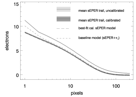
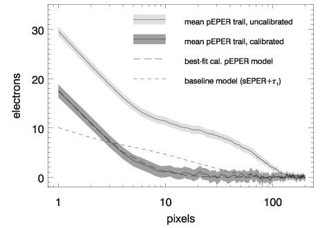
Figure 10 shows the resulting “uncalibrated” trail profiles for the sEPER (upper panel) and pEPER (lower panel) measurements in the G quadrant (eol radiation dose), at a flatfield exposure time corresponding to an average of $1018$ signal electrons per pixel. These are the upper solid lines with light grey shading denoting the propagated standard errors from the repeated experiments. Effects in the readout electronics mimic CTI. We correct for the electronic effect by subtracting the average trail in the unirradiated quadrants (E for pEPER, and E and H for sEPER). The resulting “calibrated” trail profiles and their uncertainties are presented as the lower solid lines and dark grey shadings in Fig. 10. The calibration makes a small correction to the sEPER trail which is dominated by slow traps, yielding a significant signal out to $\sim\!60$ pixels. On the contrary, the electronic effect accounts for $1/3$ of the uncalibrated pEPER trail even in the first pixel, and for all of it beyond the tenth. Thus the $S/N$ in the calibrated trail is much lower.

A.2 The well fill power $\beta$

Table 4: The same as Table LABEL:tab:traps, but for the best-fit models shown in Fig. 10. The baseline well fill power is $\beta_{0}\!=\!0.58$.

best-fit sEPER model	$i\!=\!1$	$i\!=\!2$	$i\!=\!3$
Trap density $\rho_{i}$ [px-1]	$0.01$	$0.03$	$0.90$
Release timescale $\tau_{i}$ [px]	$0.8$	$3.5$	$20.0$
best-fit pEPER model	$i\!=\!1$	$i\!=\!2$	$i\!=\!3$
Trap density $\rho_{i}$ [px-1]	$0.13$	$0.25$	$--$
Release timescale $\tau_{i}$ [px]	$1.25$	$4.4$	$--$

In a volume-driven CTI model, the cloud of photoelectrons in any given pixel is assumed to fill up a height within the silicon that increases as electrons are added (Eq. 12). The growth of the cloud volume is governed by the term $\left(\frac{n_{\mathrm{e}}}{w}\right)^{\beta}\sum_{i}\rho_{i}$ in Eq. (12), with the full-well depth $w\!=\!84700$ limiting the maximum number of electrons in a pixel. There is no supplementary buried channel in the CCD273, which for HST/ACS leads to the first $\sim 100$ electrons effectively occupying zero volume (Massey et al. 2010).

Figure 12: Trail profiles corresponding to our trap models. Upper left panel: Trails for models in which the densities $\rho_{i}$ are modified by a factor $0.9$ (red) or $1.1$ (blue). This is applied to: the fast traps $\rho_{1}$ (dashed lines); the medium traps $\rho_{2}$ (long-dashed lines); the slow traps $\rho_{3}$ (dot-dashed lines); $\rho_{1}$ and $\rho_{2}$ (triple dot-dashed lines); all traps (dotted lines). Upper right panel: The same, but relative to the baseline model. Lower left panel: Trails for trap models in which the release time scales $\tau_{i}$ are modified by a factor $0.7$ (red) or $1.4$ (blue). The line code is the same as above. Solid lines show models in which not only all the $\tau_{i}$ are changed, but also the $\rho_{i}$ adjusted such that the first pixel matches the baseline trail profile (Sect. 5.4.4). Lower right panel: The same, but relative to the baseline model.

We use measurements of the integrated EPER as a function of input signal to constrain the well fill power $\beta$ of the trapping model. Our simulated galaxies are faint; so we restrict ourselves to the four lowest signal levels measured in the laboratory, with up to $\sim\!1000$ electrons. The input signal is measured as the average count difference between the flatfield and overscan regions, corrected for the CCD gain.

Figure 11 shows the CTI trails from Fig. 10, integrated over the first $12$ pixels. We checked that integrating over up to the full overscan region length of $200$ pixels does not change the results drastically. In the sEPER data (upper panel of Fig. 11), the unirradiated quadrants E and H (open squares and diamonds) exhibit very small trail integrals (caused by the readout electronics); one order of magnitude smaller than in the irradiated quadrants F and G (open circle and triangle). Hence, calibrating out the instrumental effect by subtracting the arithmetic average from the E and H quadrants yields only a small correction to the F and G trail integrals. To these calibrated sEPER measurements (filled circle and triangle), we fit linear relations in log-log-space using the IDL fitexy routine and measure $\beta_{\mathrm{F,cal}}\!=\!0.49\pm 0.04$ and $\beta_{\mathrm{G,cal}}\!=\!0.58\pm 0.03$.

We repeat this procedure for the pEPER measurements where the unirradiated E quadrant shows a similar EPER integral than the irradiated F, G, and H quadrants (lower panel of Fig. 11). Thus, the pEPER and sEPER integrals may yield similar values as a function of signal, but for pEPER the low $S/N\!\!\ll\!1$ causes large uncertainties. Consequently, $\beta$ is not well constrained, with $\beta_{\mathrm{F,cal}}\!=\!0.66\pm 0.53$, $\beta_{\mathrm{G,cal}}\!=\!0.61\pm 0.36$, and $\beta_{\mathrm{H,cal}}\!=\!0.61\pm 0.89$, but they agree with the sEPER results.

In conclusion, we adopt a baseline well-fill power of $\beta_{0}\!=\!0.58$ for our further tests, based on the precise sEPER result for the full radiation dose.

A.3 From trail profiles to trap parameters

To constrain the trap release time-scales $\tau_{i}$ and trap densities $\rho_{i}$, we make use of the two signal levels of $\sim\!360$ electrons and $\sim\!1000$ electrons that bracket the number of electrons we expect to be found in a typical faint Euclid galaxy. These are the two highest data points in Fig. 11. We compare the average, measured, calibrated trails from the irradiated quadrants (examples for the G quadrant are presented in Fig. 10) and compare them to the output a one-dimensional version of our Massey et al. (2014) clocking routine produces given trap densities $\rho_{i}$ and release timescales $\tau_{i}$, and under circumstances close to the laboratory data (i.e. a $200$ pixel overscan region following a $2048$ pixel flatfield column of $1018$ signal electrons). The fitting is performed using the MPFIT implementation of the Levenberg-Marquardt algorithm for nonlinear regression (Markwardt 2009; Moré 1978).

Fitting a sum of exponentials is remarkably sensitive to noise in the data because the parameters ($\tau_{i}$ and $\rho_{i}$) we are probing are intrinsically correlated. We assess the robustness of our results by repeating the fit not only for the two (three) irradiated sEPER (pEPER) quadrants at two signal levels, but for a wide range of trail lengths ($60\!<\!K\!<\!150)$ we consider, and with and without adding a constant term.

There are several possible trap species as defined by their $\tau_{i}$ that show up in our data set. We rule out those of very low densities and consider the frequent “species” whose time-scales are within a few percent of each other as one. Still, this leaves us with more than one contesting family of trap species that yet give similar trails in some of the quadrant/signal combinations. Because, at this stage, our goal is to derive a plausible baseline model rather than pinpointing the correct trap species, we filter for the most common $\tau_{i}$ and give precedence to the higher-$S/N$ data (sEPER, end-of-life dose, $1000$ signal electrons). The resulting best-fit models are shown in Table LABEL:tab:models and Fig. 10. The actual baseline model (Table LABEL:tab:traps; short-dashed line in Fig. 10) includes additional fast traps seen in the lower-$S/N$ data. We raise the density from $0.94$ traps per pixels to a mnemonic total of $1$ trap per pixel at end-of-life dose. More refined methods will be used to determine the trap species in a more detailed analysis of irradiated CCD273 data.

Because only $464$ pixels of the serial register in the test device were irradiated, the effective density of charge traps an electron clocked through it experiences is smaller by a factor of $464/2051$ than the actual trap density corresponding to the end-of-life radiation dose that was applied. We correct for this by quoting results that have been scaled up by a factor of $2051/(464\times 0.94)\!\approx\!4.155$.

A.4 Example CTI trails

Figure 12 shows, for the largest deviations from the baseline trap model we consider, their effect on the shape of the CTI trails. Using our CTI model, we simulated the trail caused by a single pixel containing a signal of $\sim\!1000$ electrons, comparable to a hot pixel in actual CCD data.

References

- Anderson & Bedin (2010) Anderson J., Bedin L. R., 2010, PASP, 122, 1035
- Bertin & Arnouts (1996) Bertin E., Arnouts S., 1996, A&AS, 117, 393
- Bristow (2003) Bristow P., 2003, Instrument Science Report CE-STIS-2003-001; ArXiv astro-ph/0310714
- Casella & Berger (2002) Casella G., Berger R. L., 2002, Statistical Inference, 2nd edn. Duxbury
- Cropper et al. (2013) Cropper M. et al., 2013, MNRAS, 431, 3103
- Cropper et al. (2014) Cropper M. et al., 2014, in Proc. SPIE, Vol. 9143, 9143 0J
- Endicott et al. (2012) Endicott J. et al., 2012, in Proc. SPIE, Vol. 8453, 8453 03
- Kacprzak et al. (2012) Kacprzak T., Zuntz J., Rowe B., Bridle S., Refregier A., Amara A., Voigt L., Hirsch M., 2012, MNRAS, 427, 2711
- Kaiser, Squires & Broadhurst (1995) Kaiser N., Squires G., Broadhurst T., 1995, ApJ, 449, 460
- Kitching et al. (2012) Kitching T. D. et al., 2012, MNRAS, 423, 3163
- Laureijs et al. (2011) Laureijs R. et al., 2011, ArXiv astro-ph.CO/1110.3193
- Leauthaud et al. (2007) Leauthaud A. et al., 2007, ApJS, 172, 219
- Lindegren et al. (2008) Lindegren L. et al., 2008, in IAU Symposium, Vol. 248, IAU Symposium, Jin W. J., Platais I., Perryman M. A. C., eds., pp. 217–223
- Markwardt (2009) Markwardt C. B., 2009, in ASP Conference Series, Vol. 411, Astronomical Data Analysis Software and Systems XVIII, D. A. Bohlender, D. Durand, & P. Dowler, ed., pp. 251–255
- Marsaglia (1965) Marsaglia G., 1965, Journal of the American Statistical Association, 60, 193
- Marsaglia (2006) Marsaglia G., 2006, Journal of Statistical Software, 16, 1
- Massey (2010) Massey R., 2010, MNRAS, 409, L109
- Massey et al. (2013) Massey R. et al., 2013, MNRAS, 429, 661
- Massey et al. (2014) Massey R. et al., 2014, MNRAS, 439, 887
- Massey et al. (2010) Massey R., Stoughton C., Leauthaud A., Rhodes J., Koekemoer A., Ellis R., Shaghoulian E., 2010, MNRAS, 401, 371
- Melchior & Viola (2012) Melchior P., Viola M., 2012, MNRAS, 424, 2757
- Miller et al. (2013) Miller L. et al., 2013, MNRAS, 429, 2858
- Moré (1978) Moré J. J., 1978, in Lecture Notes in Mathematics, Vol. 630, Numerical Analysis, Springer-Verlag Berlin Heidelberg, pp. 105–116
- Murray et al. (2012) Murray N. J., Holland A. D., Gow J. P. D., Hall D. J., Tutt J. H., Burt D., Endicott J., 2012, in Proc. SPIE, Vol. 8453, 8453 16
- Prod’homme et al. (2012) Prod’homme T., Holl B., Lindegren L., Brown A. G. A., 2012, MNRAS, 419, 2995
- Prod’homme et al. (2014) Prod’homme T., Verhoeve P., Kohley R., Short A., Boudin N., 2014, in Proc. SPIE, Vol. 9154, 9154 09
- Refregier et al. (2010) Refregier A., Amara A., Kitching T. D., Rassat A., Scaramella R., Weller J., Euclid Imaging Consortium f. t., 2010, ArXiv astro-ph.IM/1001.0061
- Refregier et al. (2012) Refregier A., Kacprzak T., Amara A., Bridle S., Rowe B., 2012, MNRAS, 425, 1951
- Rhodes et al. (2010) Rhodes J., Leauthaud A., Stoughton C., Massey R., Dawson K., Kolbe W., Roe N., 2010, PASP, 122, 439
- Rhodes, Refregier & Groth (2001) Rhodes J., Refregier A., Groth E. J., 2001, ApJ, 552, L85
- Schneider (2006) Schneider P., 2006, ”Weak Gravitational Lensing” in: Gravitational Lensing: Strong, Weak and Micro: Saas-Fee Advanced Courses, Volume 33 . Springer-Verlag Berlin Heidelberg, p. 269 ff.
- Short et al. (2013) Short A., Crowley C., de Bruijne J. H. J., Prod’homme T., 2013, MNRAS, 430, 3078
- Short et al. (2014) Short A. D. et al., 2014, in Proc. SPIE, Vol. 9154, 9154 0R
- Smith et al. (2012) Smith L. J. et al., 2012, in American Astronomical Society Meeting Abstracts, Vol. 219, American Astronomical Society Meeting Abstracts, p. 241.01
- Tin (1965) Tin M., 1965, Journal of the American Statistical Association, 60, 294
- Verhoeve et al. (2014) Verhoeve P., Prod’homme T., Oosterbroek T., Boudin N., Duvet L., 2014, in Proc. SPIE, Vol. 9154, 9154 16
- Viola, Kitching & Joachimi (2014) Viola M., Kitching T. D., Joachimi B., 2014, MNRAS, 439, 1909