Freeze-In Dark Matter
with
Displaced Signatures at Colliders
Raymond T. Co, Francesco D’Eramo, Lawrence J. Hall and Duccio Pappadopulo
Berkeley Center for Theoretical Physics, Department of Physics,
and Theoretical Physics Group, Lawrence Berkeley National Laboratory,
University of California, Berkeley, CA 94720, USA
Abstract
Dark matter, , may be generated by new physics at the TeV scale during an early matter-dominated (MD) era that ends at temperature . Compared to the conventional radiation-dominated (RD) results, yields from both Freeze-Out and Freeze-In processes are greatly suppressed by dilution from entropy production, making Freeze-Out less plausible while allowing successful Freeze-In with a much larger coupling strength. Freeze-In is typically dominated by the decay of a particle of the thermal bath, . For a large fraction of the relevant cosmological parameter space, the decay rate required to produce the observed dark matter abundance leads to displaced signals at LHC and future colliders, for any in the range and for values of accessible to these colliders. This result applies whether the early MD era arises after conventional inflation, when is the usual reheat temperature, or is a generic MD era with an alternative origin. In the former case, if is sufficiently large to be measured from kinematics, the reheat temperature can be extracted. Our result is independent of the particular particle physics implementation of , and can occur via any operator of dimension less than 8 (4) for a post-inflation (general MD) cosmology. An interesting example is provided by DFS axion theories with TeV-scale supersymmetry and axino dark matter of mass GeV to TeV, which is typically overproduced in a conventional RD cosmology. If is the higgsino, , Higgs, W and Z particles appear at the displaced decays, and . The scale of axion physics, , is predicted to be in the range GeV and, over much of this range, can be extracted from the decay length.
1 Introduction
In the early universe, when the background radiation had a temperature from eV to MeV, the energy density was dominated by radiation. How far back did this radiation dominated (RD) era extend? When inflation ended, provided the inflaton decays were not extremely rapid, there was an era of matter domination (MD) which ended at the reheat temperature . It is commonly assumed that is very high, many orders of magnitude above the TeV scale, but observationally the most stringent constraints are from the effective number of neutrino species from CMB measurements, MeV [1], and from Big Bang Nucleosynthesis [2]. This early MD era could extend for many decades in temperature above , and include the TeV epoch. There are several alternative origins for a long early MD era, including long-lived heavy particles that were once in thermal equilibrium and oscillating fields composed of light bosons. When the MD era results from inflation it has an evolution that is purely Non-Adiabatic in character, giving a MDNA era, as shown in Fig. 3. The more general MD era splits into two, beginning with Adiabatic evolution, MDA, and ending with MDNA, as illustrated in Fig. 1.
In this paper we explore the consequences of having the dark matter abundance determined by reactions during an early MD era. This profoundly changes the abundance compared to the conventional assumption of dark matter genesis during the RD era for two reasons. Firstly the time-temperature relation is changed so that any given temperature occurs at earlier times and secondly, once the genesis reactions stop, the comoving abundance of dark matter is diluted by entropy production. The second effect dominates, so that the MD era results in a depletion of dark matter relative to the usual RD result; by a factor for Freeze-Out during MDNA[3, 4, 5], where is the Freeze-Out temperature, and by a factor for Freeze-Out during MDA [6] where is the temperature at which begins. This factor is likely very small, suggesting a dark matter mass much larger than the TeV scale. In this paper we focus on TeV scale physics as the origin of dark matter, as this could be probed at colliders, and therefore we seek an alternative to Freeze-Out, as Freeze-Out during a MD era is unlikely to yield sufficient dark matter.
Particle dark matter requires an addition to the Standard Model: a cosmologically stable particle of mass . How is the abundance of determined? The Freeze-Out mechanism results if has sufficient interactions with the known particles that it is in thermal equilibrium at temperatures of order . As drops below , tracks a Boltzmann distribution for a while but, as it becomes more dilute, its annihilation rate drops below the expansion rate and it freezes out of thermal equilibrium. This mechanism has great generality, applying to a wide range of theories where the interactions of are sufficient to put it in thermal equilibrium at . Furthermore, it is highly predictive since it is an IR dominated process - it does not depend on any physics at energy scales above its mass. Indeed, Freeze-Out during the RD era suggests is broadly of order a TeV and that has an interaction rate that can lead to signals at both collider detectors and direct and indirect detection experiments.
Freeze-In provides another general production mechanism and results when the interactions of are insufficient to bring it into thermal equilibrium [7].111We do not consider the case of dark matter arising from decay of the matter that dominates the energy density during the MD era [8]. At temperatures above these feeble interactions allow the production of from decays or scatterings of some bath particle of mass at rate . This produces a yield of particles at time of
| (1) |
which is IR dominated when the interactions between and are of dimension 4 or less. Taking to be the lightest observable sector particle carrying the stabilizing symmetry, the production rate becomes Boltzmann suppressed below , so that the dominant contribution to arises at . For , the yield grows towards its equilibrium value, but it never reaches equilibrium, and this Freeze-In towards equilibrium stops once drops below . Decays generally dominate over scatterings, so that in this paper we study the reaction
| (2) |
where is one or more Standard Model particles.
When Freeze-In occurs during the RD era, the value of the lifetime that leads to the observed dark matter abundance is of order for of order the weak scale. This leads to interesting signals of long-lived stopped particles at colliders if carries electric or color charge [7], but not if is neutral. The interaction between and is described by a very small coupling of order , as shown by the blue curve of Fig. 4.
In this paper we study Freeze-In during an early MD era, requiring to be less than , and find that the lifetime, , is reduced. Freeze-In via scattering during the MDNA era was studied in [4, 5], whereas Freeze-in via decays for goldstino DM was studied in Ref.[9]. The reduction in arises because the relevant time scale that appears in (1) is smaller in the MD era than in the RD era and because the produced yield is subsequently diluted by entropy production. Both effects require an increase of the rate appearing in (1). In a model-independent analysis, we find that the required depends on two particle physics parameters and two cosmological parameters , where appears only if the MD era has a MDA portion, in which case it represents dilution. For Freeze-In during a MDNA era we show our results in the two panels of Fig. 6 for values of relevant for LHC and future hadron colliders, respectively. The decay length in this case is function of the reheat temperature only. If we also allow a MDA era then we have contours for in the plane, as show in Figs. 8 and 9. Over a large portion of the parameter space for Freeze-In during the MD era via (2), these decays can be probed at colliders as they lead to exotic signals displaced from the primary vertex. This result is remarkably general, applying to a wide range of dark matter masses, , and a wide range of interactions that induce the decay (2)222Our results also apply to , with containing exotic non Standard Model particles, followed by rapid decays . The Freeze-In yield and the collider decay length are then both determined by .. For Freeze-In during the MDA era, any interaction of dimension 4 or less is sufficient, while the extreme UV-insensitivity of the MDNA era allows any interaction of dimension less than 8.333Our results also apply if is part of a hidden sector and FI dominates dark matter production [10]. While the interaction is still feeble, the strength is several orders of magnitude larger than in the RD case; for example, a coupling of order for the dimension 4 case, as in the red curve of Fig. 5.
The displaced collider signals have a size depending on the production rate of and a character depending on the identity of and . For color and charge neutral, possibilities for include giving a variety of non-prompt decays. Using Run I data, LHC experiments have placed limits on displaced vertices [11, 12], displaced jets [13, 14] and displaced leptons [15, 16]. However, some of these analyses have assumed particular forms for the signal, and may not be sensitive to, or optimized for, Freeze-In. For example, it would be interesting to search for displaced signals involving a Higgs or boson, as arise from . For carrying color and/or charge, includes giving decays from long-lived particles stopped in the detector [17, 18].
Axino dark matter in supersymmetric DFS theories of the QCD axion provides an interesting example of Freeze-In. With Freeze-In during the conventional RD era too much dark matter is generically produced, unless theories are crafted to have very high axion scales, , or very low axino masses. However, for Freeze-In during the MD era, axinos account for the observed dark matter for in the range GeV and axino masses in the GeV to TeV range. Furthermore, as shown in Figs. (10) and (11), over a large fraction of the parameter space not excluded by axion overproduction and white dwarf constraints, there are displaced signals at colliders that arises from the higgsino decays that induce the cosmological abundance, and .
2 An Early Matter Dominated Era
In this section we review the evolution of the universe during an early Matter Dominated era, MD, and study the parameter space of such a cosmology relevant for Freeze-In (FI) of dark matter. We consider an FRW cosmology with two components: Radiation and unstable Matter , that decays to radiation with a decay rate . The radiation is thermal at temperature and has energy density
| (3) |
where counts the effective number of relativistic species at , including particles from the Standard Model and beyond. The matter can be fermonic or bosonic and, in the era of interest to us, is not thermally coupled to the radiation. The particles might have been in thermal equilibrium at an earlier epoch when they were relativistic, so that they have a number density comparable to that of the relativistic species, or they might arise from a classical oscillating bosonic field, as with inflatons or moduli, in which case their number densities could be much larger. When is of order the MeV scale have decayed and the universe is in the conventional Radiation Dominated era, RD, but at earlier times we insist that the initial density of is sufficiently large that there is a long matter dominated era.
The Boltzmann equations governing the evolution of the energy densities are
| (4) |
where is the Hubble parameter. 444The second line of Eq. (4) is derived from the first law of thermodynamics under the assumption that the equation of state is satisfied. Strictly speaking, this is not exactly true when the temperature is near the mass of any of the particles in the thermal bath. We verified that the corrections to the equation of state are small and they only affect the final results by a few percent. Therefore, we take a constant value of in our numerical study. Freeze-in is dominated at temperatures of the order of the weak scale, so we take , accounting for the full Standard Model degrees of freedom. The solutions to these Boltzmann equations depend on the initial densities and . At times earlier than , the effect of decays on can be ignored, giving
| (5) |
where is the Robertson-Walker scale factor and GeV. There are two contributions to the radiation energy density, the first is the red-shifted initial density while the second, proportional to , arises from decay.
This solution is illustrated in Figure 1 for sufficiently small that the universe starts in an early radiation dominated era, RD′.
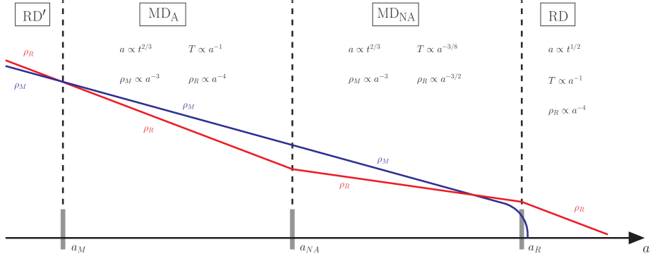
It transitions at to the early MD era, which ends at reheat, , when decay and drops to zero. The MD era is divided into two regimes. In the earliest one is dominated by red-shifted initial radiation, so that the second term in can be ignored and the evolution is Adiabatic (the MDA era). The second regime has dominated by radiation from decays, and hence the evolution is Non-Adiabatic (the MDNA era); the first term in can be ignored so . If is sufficiently large the universe evolves through both MD regimes; otherwise there is only a MDNA regime. The transition between these two types of cosmology occurs at
| (6) |
2.1 General MD Histories Relevant for Freeze-In
In this paper we study Freeze-In of dark matter during this MD era. Taking matches on smoothly to the RD′ era, but it could be that the Boltzmann equations of (5) break down at some larger than , so that the MD era emerges from a non-RD era, such as inflation or topological defect domination. To be completely general we allow to be anywhere between and . (Taking gives an identical MD era to the case of , and does not have an early MD era.) Equivalently, we study all initial conditions with
| (7) |
In fact we insist that so that the MD era is not a transient phenomenon.
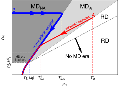
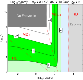
The set of cosmological histories of interest to us is shown shaded in Figure 2, and splits into two according to whether the evolution is initially MDA (light gray) or MDNA (dark gray). The region above the dashed line which is initially RD′ will evolve to give the same MD era as histories on the boundary between initially RD′ and initially MDA. Two particular histories are illustrated by the red and blue trajectories having initial energy densities A and B. Point A has and corresponds to in Figure 1, leading to both Adiabatic and Non-Adiabatic evolution. Point B has . In this case, those that decay much earlier than rapidly increase the radiation density to , leading to a MD era that is purely Non-Adiabatic. The horizontal part of the blue trajectory is covered very quickly so that the MDNA evolution occurs on the non-horizontal part of the blue trajectory. For fixed , the possible histories with purely Non-Adiabatic evolution can be described by , which labels points along the line of non-adiabatic evolution. Histories having both evolutions are described by , corresponding to points in the region with light shading.
Histories with , such as the blue trajectory in Fig. 2, could emerge from an inflationary era with interpreted as the inflaton, which starts to oscillate at , as illustrated in Fig. 3.
2.2 Evolution of time, temperature and energy density
For the purposes of studying Freeze-In during the MD era, we lose no generality in considering histories with (corresponding to , such as point A in Figure 2) since, in the late part of their evolution, they include all other histories that have larger . In particular, solutions with equal initial conditions always contain a MDNA phase at late times; therefore they also cover histories with only a MDNA era (up to the very quick beginning of it, shown on the horizontal blue line in Fig. (2)). Hence the three dimensional parameter space () may be collapsed to two (). The evolution of time and temperature in these histories, relevant for physical processes, is discussed below and the two parameters may be taken as , the temperatures at the beginning and end of the MD era. They are related to () by and .
During the entire MD era the age of the universe is . During the MDA regime is constant. For a simple pedagogical discussion, we will assume a constant so that the energy density is
| (8) |
and in this regime the time-temperature relation has the parametric form
| (9) |
The universe transitions from adiabatic to non-adiabatic evolution when the two terms in of (5) are comparable, at time555The symbol indicates approximations resulting from complicated behaviors during transition regions between eras, while the symbol indicates that, in addition, numerical constants have been dropped.
| (10) |
with and , and at temperature
| (11) |
In Fig. 2, points along the boundary separating the initially MDA and MDNA regions can be labeled by . For histories resulting from inflation there is no MDA era, rather the history begins at , which is identified with
| (12) |
where is the energy scale of inflation. For this case it is convenient to take the independent variable as instead of .
During the MDNA regime is constant so that the energy density is
| (13) |
where has been normalized so that it is equal to at . This gives a time temperature relation
| (14) |
| (15) |
The final RD era is reached when and . Including a numerical factor, (14) at this transition gives
| (16) |
Above eV the universe was radiation dominated and it is frequently assumed that this RD era began at extremely high temperatures, as high as the energy scale of conventional inflation, , which could be as large as GeV. However, in the cosmology discussed here, the universe had a long MD era from to . Observational constraints are very mild: MeV from CMB and BBN and . Even in the case that this early MD era arose from the conventional inflaton, and hence was purely MDNA, it could have lasted for many decades in temperature from as low as 3 MeV to . If the DM abundance was determined during the MD era we expect significant changes in predictions compared to the RD case for two reasons. The DM yield depends on the Hubble parameter at production ( for FO and for FI) and at any temperature in the MD era H is larger than at the same temperature in the RD era by an amount that can be as large as when . However this is overwhelmed by dilution effects subsequent to DM production, which reduces the yield by as much as . For the production of TeV-scale dark matter in a long MD era this is typically catastrophic for FO since the abundance becomes too low, but for FI it has the interesting feature of enhancing the required couplings of the weakly interacting state to yield displaced signals at colliders.
3 Freeze-In During an Early MD Era
We consider Freeze-In (FI) production of dark matter during the early MD era via the decay . is the lightest observable sector particle that carries the stabilizing symmetry, is the dark matter and is one or more Standard Model particles. In addition to FI, there is a Freeze-Out (FO) population of that eventually decays to . In this Section we focus on FI, deferring FO to Appendix B where we show that in the early MD era it is typically negligible.
The number density evolution of is described by the Boltzmann equation [7]
| (17) |
with the width of and the first and second modified Bessel functions of the 2nd kind. The equilibrium number density obtained using Maxwell-Boltzmann statistics reads
| (18) |
At high temperatures () we recover the abundance for a relativistic species, whereas at low temperatures () the number density has the Maxwell-Boltzmann exponential suppression. For this reason, the FI production of is dominated at temperatures .
If FI occurs during the RD era, the Boltzmann equation (17) can be easily solved [7] giving a final yield for
| (19) |
where is the entropy density. Observations fix the DM density but the yield is fixed once the mass of is known using
| (20) |
which is close to the usual temperature of matter radiation equality, . We can thus rewrite eq. (19) as
| (21) |
The coupling , defined by
| (22) |
must be very small to avoid overclosure. For the reference masses and number of spin states shown in (21) the observed DM density results for .
In Fig. (4) we show the FI solutions for the DM yield , with time variable . We show three different lines corresponding to three different values of (namely three different decay widths as in Eq. (22)). In all cases we see that the process is maximally active at temperatures of order . For the reference parameters of (19), the blue line reproduces the observed DM density, whereas the brown and red lines overproduce the amount of dark matter. In particular, the red line reaches an asymptotic value of which is the equilibrium value , and above this point the approximation that DM arises from FI through the decay in Eq. (2), and without the inverse reaction, breaks down.
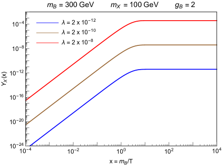
The FI abundance depends on the cosmological evolution at and after FI. The solution of the Boltzmann equation (17) is given in Appendix A for an arbitrary cosmological evolution in Eqs. (58) and (59). In this section we apply this to the cosmological backgrounds discussed in the previous section, with energy density evolving according to the Boltzmann equation (4). These cosmological backgrounds depend in general on three parameters, and (or equivalently ). In the next subsection we study the case of FI during the MDNA era, which is particularly simple because there is no dependence on or and the results can be displayed as a function of .
3.1 Freeze-In during Non-Adiabatic evolution
Freeze-In during MDNA occurs between and , as shown in Fig. 1, and the final DM density depends on only one parameter of the background, the reheat temperature . This includes the important example of FI during reheating after inflation, as sketched in Fig. 3. In this case inflation could be the conventional one with more than 60 e-foldings with the matter M identified as the usual inflaton, or it could be a later era of inflation with fewer e-foldings.
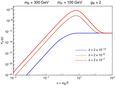
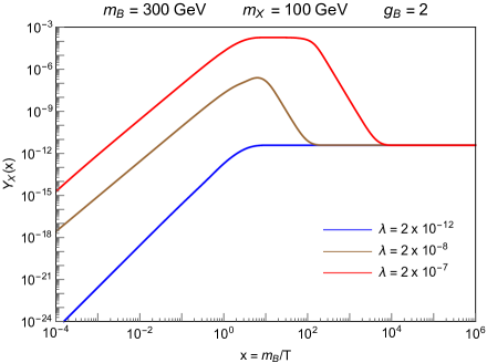
The FI yields are shown in Fig. 5 for three different values of the decay width
| (23) |
In each case we choose in such a way that we reproduce the observed DM abundance. The values of span a wider range than the case of Fig. 4 since Freeze-In during a MD era allows for larger couplings. The blue line has , so that FI occurs during the RD era. As is increased, the FI process becomes more powerful, as illustrated by the brown and red lines, and to obtain the observed DM abundance much lower values of must been taken, so that the abundance is diluted by entropy production after FI. However, it is not possible to arbitrarily increase and still be in the Freeze-In regime. For sufficiently large , the peak of the functions in Fig. 5 will reach the equilibrium value and FI is no longer the applicable production mechanism. For reference values () this gives a lower limit . At the same time we have to keep ; otherwise FI occurs during the RD era and there would be no dilution.
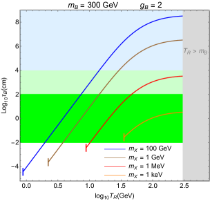
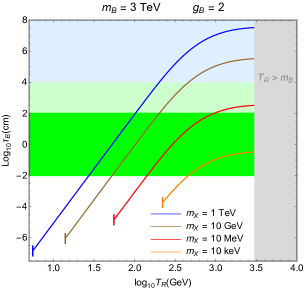
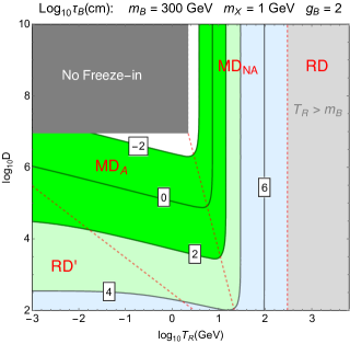
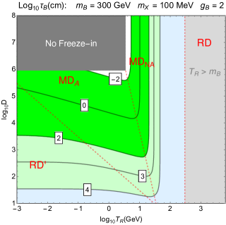
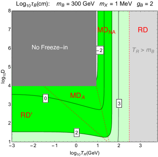
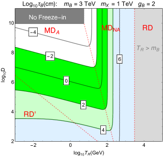
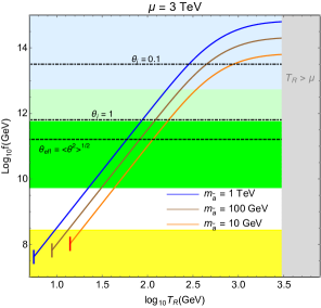
The decay length necessary to reproduce the observed DM abundance is shown in Fig. 6 as a function of . The left (right) panel is for a value of () relevant for the LHC (future colliders) and four curves are shown in each, giving results for a wide range of . Signal regions for various displaced events at colliders are given by shaded horizontal bands, as described in Table 1. The stopped particle decay signal is absent if is color and electric charge neutral.
| Shaded region | Decay length | Signature from LOSP | Neutral | Charged |
|---|---|---|---|---|
| Dark green | Displaced vertices | |||
| Light green | Displaced jets/leptons | |||
| Light blue | Stopped particle decays | X |
3.2 Freeze-In during Adiabatic or Non-Adiabatic evolution
We extend the previous discussion to the more general framework of Fig. 1, which also allows for a period of adiabatic evolution during the MD era. The full parameter space of the cosmological background is () but, as discussed in Section 2, for FI there is no loss of generality in taking . The parameter space may then be taken as , where is the temperature at the beginning of the MD era. We trade for another parameter, the dilution , where and are the entropy per comoving volume before and after the matter decay.
We consider the same three values of the coupling as in Eq. (23), and we choose the dilution factor and the reheat temperature to reproduce the observed DM abundance. There is some degeneracy in the process, and for the purpose of illustration we fix
| (24) |
The solutions are shown in Fig. 7. This time we notice a different behavior between the brown and red lines. The reason is a consequence of our choice of : for the (brown) red line the Freeze-In happens during the (non-)adiabatic matter dominated era.
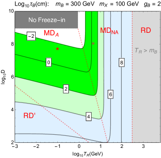
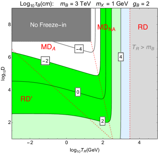
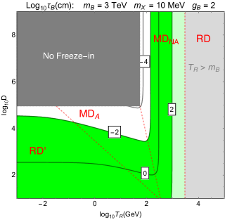
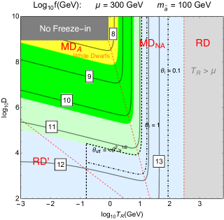
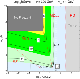
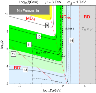
Figs. 8 and 9 provide a complete exploration of FI in the plane, with results shown for different . The LOSP mass values of (Fig. 8) and (Fig. 9) are chosen to be relevant for LHC and a future collider, while values of are chosen to span the very wide range of possible values that is consistent with FI. Remarkably, the displaced vertex region, shaded in green, is always within the FI domain and covers a substantial part of the parameter space where the observed DM results from FI.
3.3 Analytic Approximation to Freeze-In Abundance
Many features of the numerical results presented in the previous two sub-sections can be understood from simple analytic approximations. The FI abundance of generated during a Hubble doubling temperature at during era is
| (25) |
where is the total rate of production at temperature . For clarity numerical factors are dropped in this sub-section, unless they are very large. The age of the universe at is
| (26) |
with running over the (RD, MDNA, MDA, RD′) eras, with RD the usual RD era at and RD′ the early one at . When FI is induced by an operator of dimension 4, the rate of X production is given by
| (27) |
at . The upper entry of the vector is for decays, with the Lorentz boost factor, while the lower entry is for scatterings.
This analytic yield approximates the solution to the Boltmann equations, , for , where dilution does not have a large effect. For the case of decays, the power laws in the various eras are . At , the RD, MDNA and MDA slopes are visible in Figs 4, 5 and 7, respectively. (In Fig. 5 the blue curve starts with MDNA behavior, but the slope decreases as approaches unity where FI occurs during the RD era. In Fig. 7 the blue curve has , so that there is no MD era and the slope reflects RD.)
The contribution to the DM yield today from FI production when the universe had temperature and was in era is
| (28) |
where is the dilution factor from non-adiabatic decays of during the MDNA era between and
| (29) |
During the MDNA era, Eq. (13) shows that , so that the dilution factor of scales as . As the temperature increases to the dilution reaches which by Eq. (15) is , the constant dilution factor for production in the MDA and RD′ eras.
Combining Eq. (25) — Eq. (29) gives
| (30) |
For decays and scatterings in all eras, FI via interactions of dimension 4 is IR dominated at . Decays and scatterings then give contributions with the same scaling behavior, giving a total yield today of
| (31) |
Including numerical factors the decay contribution is larger than the scattering one, which is why we have included only decays in our numerical analysis.
For FI during the MDNA era, Eq. (30) shows that IR domination is extreme, with a power behavior of with , so that FI production is maximized at temperature with . The high power dependence leads to an abundance from FI on the exponential tale of the Boltzmann distribution for that is enhanced by a large factor , of order , compared to FI at . Similarly, in Fig 5 peaks at . The behavior for the yield during the MDNA era, shown in Eq. (31), leads to the straight lines of slope 7 in Fig. 6.
For FI during the MDA era, Eq. (31) shows that the yield is proportional to . so that in the MDA region of Fig. 8 the contours of constant have constant. On the other hand, in the MDNA region of Fig. 8 the contours are vertical since they depend only on and not on . The boundary between the MDNA and MDA eras is given by
| (32) |
The boundary between the MDA and RD′ eras is given by .
For any , knowing which era dominates FI allows the contours of Fig. 8 to be normalized by requiring the observed DM abundance
| (33) |
so that the decay rate prediction scales as
| (34) |
Including relevant numerical factors, these scaling law predictions can be written as
| (35) | |||||
| (36) | |||||
| (37) | |||||
| (38) |
leading to the behaviors of Figs 6, 8 and 9. The value of the coupling required for dark matter genesis during era can be estimated from (34).
For FI during era to give the observed DM abundance, the peak abundance reached before dilution is
| (39) |
with evaluated at for the MDNA era. This result for breaks down for MDNA, MDA, RD′ when it gives a result larger than the equilibrium abundance, , so that FI is no longer the appropriate description of the DM production mechanism. This happens for
| (40) |
and corresponds to the shaded regions labelled “No Freeze-in” in Figs. 8 and 9. Substituting these bounds into (34) one discovers that the couplings , while much larger than , are small.
3.4 Freeze-In from higher dimensional operators
As the dimension of the interaction inducing increases, so the scattering cross section for this transition grows more rapidly with temperature. This has the tendency to convert FI from an IR process dominated by temperatures near to a UV one, dominated at some temperature . For example, a operator with coefficient inducing FI during era leads to a total yield today of
| (41) |
replacing the result (31) for . However, in the case of the MDNA era, the IR dominance for is so strong that the scattering remains IR dominated for all [5]. The FI result is obtained from the case by replacing with . The feeble strength of the interaction necessary for dark matter to originate from FI can be understood as arising from a high mass scale of size
| (42) |
The resulting lifetime, , has the same form as for shown in Fig. 6, except the normalization is changed because FI may be dominated by scattering rather than decays and as increases the enhancement factors decrease.
4 Supersymmetric Theories with Axino Dark Matter
The QCD axion is the most elegant solution to the well known CP problem of strong interactions. If supersymmetry is relevant to our universe the details of how the axion solution is implemented can play a crucial role in electroweak physics. This happens if the operator is charged under the Peccei-Quinn (PQ) symmetry whose breaking delivers the QCD axion. If this is the case the usual supersymmetric -term is not allowed in the superpotential but must be generated after PQ breaking by operators of the form [20]
| (43) |
where is a dimension operator which we assume to be the product of SM gauge singlet superfields with the right PQ charges. The effective -term comes from the vev of
| (44) |
The fields that break the PQ symmetry have PQ charges and vevs and is the effective PQ breaking scale. The axion superfield
| (45) |
transforms under a PQ transformation with real parameter as . The axion supersymmetric effective field theory just below has self interactions and interactions with the Higgs supermultiplets given by [21]
| (46) |
where is the PQ charge of the operator . Expanding this Lagrangian gives
| (47) |
where . Additional terms in the Lagrangian give interactions of the axion supermultiplet with supersymmetric gauge field strengths
| (48) |
To compute axino FI we work in a basis where the coefficients get contributions only from integrating out matter, charged under both the SM gauge group and PQ symmetry, that has a mass larger than the scale .
4.1 Axino production in standard cosmology
In the limit of of unbroken SUSY, the supermultiplet in Eq. (45) contains degenerate particles, that are massless up to a small non-pertubative QCD contribution. The axino acquires a highly model dependent mass after SUSY breaking. Given its very weak interactions with visible fields, the axino could easily have dramatic consequences for cosmology regardless of where it sits in the spectrum of superpartners [22]. We take the axino to be the stable Lightest Supersymmetric Particle (LSP), compute its cosmological abundance, and discuss constraints on the theory that allow it to be dark matter. In this sub-section we assume a standard cosmological evolution, i.e. a non-adiabatic matter dominated era following inflation starting at a temperature and ending at a temperature , followed by radiation domination down to the eV era.
Axino production in the early universe can take place through different mechanisms. Out-of-equilibrium LOSP decays naturally provide cold axino dark matter [23]. Scattering and decays of particles in the primordial plasma give additional contributions to the axino relic density. This can be due to processes mediated by the super-gauge axino-gluino-gluon interaction [24] or the axino-higgsino-Higgs Yukawa coupling in DFS models [25].
Assuming , Eqs. (47) and (19) allow us to calculate the axino FI yield coming from higgsino decay . In particular the relevant dimension 4 operator in (47) gives . With and negligible mixing with the electroweak gauginos, the decay widths of the charged and neutral Dirac components are equal and given by
| (49) |
The decay widths do not depend on under the assumption of unmixed higgsinos. These widths define the higgsino lifetime by . Notice, furthermore, that if the B particle is the higgsino in Eq. (19), giving
| (50) |
An additional contribution to the yield of arises if some of the coefficient , say , are non-vanishing. This contribution is UV dominated and arises from processes of the kind where is either a gluon or a gluino and has been calculated in [26]
| (51) |
This growth with stops once exceeds the mass of the heaviest fermion carrying both SM and PQ charges [27], so that this UV contribution is highly model dependent. In contrast, the FI yield (50) is generic to all DFS theories. The axino abundance is given by the FI mechanism only if and , the thermal abundance.666An additional UV dominated contribution to the axino abundance comes from dimension 5 operator of the form . These contribution are suppressed by a factor so that they are irrelevant for weak scale supersymmetry for the values of we are going to consider.
Defining the axion decay constant, , by the interaction with the gluon field strength in the low energy effective theory, , gives
| (52) |
where is the contribution to the anomaly from non SM fields whose masses are below the scale and the last term in the sum accounts for the anomalous contribution coming from the SM quarks. For the choice of parameters made in Eqs. (50) and (51), the axino yield is very high. The observed dark matter density will be exceeded unless the axino mass is far below the supersymmetry breaking scale and/or is very large. This is especially true if , when the yield is dominated by UV scattering. Large and/or small are certainly possible, and are the conventional approach to this axino over-abundance problem, but they place severe restrictions on the theory.
The simplest theories giving the superpotential as in Eq. (43) have with dimension , giving for , so that the yields of Eqs. (50) and (51) are indeed very large. For theories with larger , a large value of yields too much axion dark matter unless the initial axion misalignment angle is adequately tuned to small values. The tree-level axino mass is bounded from above by [28], with the scale of SUSY breaking. This limit applies even taking into account the soft SUSY breaking terms [22]. This mass would be small enough to avoid any overabundance. However, this tree-level prediction can easily be spoiled. It is quite generic for the axino to pick up a mass of order the gravitino mass via higher dimensional operators coupling the axion supermultiplet to SUSY breaking fields [29]. If SUSY is broken at a high scale, as in gravity mediation, the axino will generically pick up a weak scale mass. Even for lower mediation scales there can be loop-mediated SUSY breaking contributions to the axino mass (first pointed out in Ref. [30] within the context of supergravity theories) depending on the UV completion of Eq. (47).
In this section we pursue an alternative solution to this axino-overproduction problem: we take below the higgsino mass so that FI occurs during the MD era. The FI yield (50) is then suppressed by a combination of less available time for production and subsequent dilution from entropy production, as in (31). From the above discussion we assume the axino mass is not far below the weak scale
| (53) |
The UV contribution (51) is similarly suppressed and, as discussed in the next sub-section, we will be interested in situations where it is sub-dominant. We find that axino dark matter then predicts a restricted range of and that in much of the parameter space the reactions and lead to displaced signals at colliders.
4.2 Axino Freeze-In during an early matter dominated era
Let us review the assumptions which will go into this section. We assume the strong CP problem to be solved by a supersymmetric DFS axion. The axino mass is required to be in the range of Eq. (53) and we assume the axino to be the DM. We furthermore assume for simplicity the LOSP to be a higgsino with negligible mixing with the electroweak gauginos.
We begin by requiring there are no fields charged under both the PQ and SM gauge symmetries that are heavier than the TeV scale, so that in Eq. (48) and there is no UV scattering yield from temperatures above the TeV scale. In this case, after the rescaling of Eq. (52), the higgsino decay widths depend only on ,
| (54) |
The general analysis of FI in a cosmology with an intermediate MD era performed in Sec. (3) can then be directly translated to this model using Eq. (54), for both the numerical and analytic analyses. For any point of the general parameter space depicted in Fig. (2) we are thus able to determine the value of , and hence , that gives the observed dark matter abundance.
The numerical results for axino FI are shown in Figs. (10) and (11) for FI during inflationary reheating and during a generic MD cosmology respectively. The qualitative behavior of the figures can be understood using the analytical approximations in Sec. (3.3), in particular (31), and taking for the higgsino:
| (55) | |||||
In the region to the right of the black dashed line in Figs. (10) and (11), there is an overabundance of QCD axions produced by the misalignment mechanism. This limit applies to the region of parameter space with a post-inflationary scenario [31, 32] where the PQ phase transition occurs after inflation. If is above 160 MeV the entropy generated at the end of the MD era does not dilute the axion density coming from coherent oscillations of the axion field but only the (theoretically uncertain) contribution coming from the decay of topological defects [33]. For values of below 160 MeV the misalignment contribution is strongly diluted and negligible. Notice that the red exclusion does not apply for the pre-inflationary axion scenario as one can tune the initial misalignment angle to arbitrarily small values.
The yellow shaded region in the figures corresponds to the bound coming from axion emission from white dwarfs [34]. The bound applies if the axion-electron coupling
| (56) |
is present, which is typically the case for DFS axions, and is shown for . The axion energy density bound from misalignment and the white dwarf bound depend on and are shown in Figs. (10) and (11).
The green shaded regions correspond to higgsino lifetimes that give rise to displaced signals at colliders (with the color code as defined in Tab. 1). The higgsino decays to missing energy and, depending on whether it is charged or neutral, to a boson or democratically to a Higgs or Z boson. An early study of these signals can be found in Ref. [35], a more recent analysis for LHC collisions was performed in Ref. [36]. Notice that this signal is distinguishable from the decay of the neutralino NLSP in gauge mediated models where final states containing a photon are possible while they are strongly suppressed in the axino case.
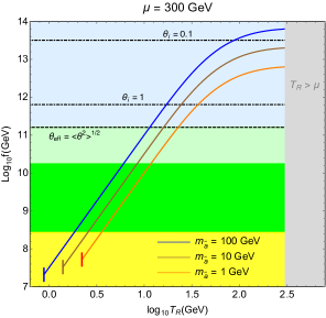
At a hadron collider, in the most favorable situation, it will be possible to measure both and from kinematical distributions and the higgsino decay width from the displaced vertex. This is enough to extract in the case of FI during post-inflationary cosmology or a corresponding curve in the plane in the case of a generic MD era. In the axino case the decay width is related to the axion decay constant and this correspondence is 1 to 1 for an unmixed higgsino as in Eq. (54). Even though the axion is not dark matter in most of the displaced vertex region, low energy experiments looking for axion-mediated long-range forces [37] can measure independently and provide a crucial verification of the framework discussed in this section.
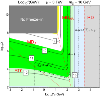
How are these results affected by going to non-minimal DFS models with matter heavier than the TeV scale inducing in (48) and (51)? For the case of the MDNA cosmology, as occurs after inflation as shown in Fig. (3), there is no change and Fig. (10) applies unaltered. In this case, even though the operator of (48) has dimension 5, it induces an axino yield that is IR rather than UV dominated, and this IR contribution is always less than that from higgsino decay. Furthermore, additional FI yields from heavy colored states are suppressed by the strong IR dominance of MDNA. However, gauge scattering axino production is UV dominated during MDA and RD′ eras, as well as during any RD era that preceded them, and further FI yields from these eras might be significant. In this case it is model-dependent whether the axino yield is dominated by FI from higgsino decays and Fig. (11) applies only if the FI contribution from higgsinos dominates.
Figs. (10) and (11) demonstrate that, in a wide range of DFS models, the dark matter can be axinos with a mass in the GeV to TeV range, with the dominant production mechanism being FI from higgsino decay during an early MD era. Over a large fraction of the parameter space not excluded by axion overproduction and white dwarf constraints, there are displace signals at colliders arising from precisely the decays that induced the cosmological abundance, and . The relevant range of is low: from the experimental lower bound up to order GeV, which can be independently explored by a variety of techniques [37].
Acknowledgments
This work was supported in part by the Director, Office of Science, Office of High Energy and Nuclear Physics, of the US Department of Energy under Contract DE-AC02-05CH11231 and by the National Science Foundation under grants PHY-1002399 and PHY-1316783. F.D. is supported by the Miller Institute for Basic Research in Science. R.C. is supported by the National Science Foundation Graduate Research Fellowship under Grant No. DGE 1106400.
Appendix A Solution of FI Boltzmann Eq. for Any History
We solve the Freeze-In Boltzmann equation (17) by employing techniques analogous to the ones used in Refs. [4, 5]. In cases where entropy is not conserved in the evolution, is not the best variable to use. We define the comoving number density, , and we use the scale factor as time variable .
The Freeze-In Boltzmann equation in terms of the new variable reads
| (57) |
The asymptotic comoving density is found by imposing the initial condition
| (58) |
The Hubble parameter is given by the Friedmann equation
| (59) |
where is the non-radiation component of the energy density and the temperature is related to the radiation energy density by Eq. (3).
For late times the comoving density approaches a constant value , and this value can be used to compute the DM density today. At the universe enters the usual RD era and we can trust entropy conservation again. Therefore, we identify a late temperature less than and evaluate and the entropy . This ratio in the subsequent evolution of the universe must be constant. We define
| (60) |
The energy density today reads
| (61) |
The contribution to the dark matter energy density reads
| (62) |
This solution is completely general and valid for Freeze-In during an arbitrary background of radiation and non-radiation components.
Appendix B Irrelevance of LOSP Freeze-Out in MD Era
So far we have not discussed the LOSP Freeze-Out (FO) contribution to the DM density. If we assume the LOSP particle to be a generic particle with a weak scale mass and couplings, and in the absence of dilution, this contribution is in the right ballpark to account for the observed DM abundance. The goal of this Section is to show that, in the displaced signal regions for FI identified above, FO is always suppressed and can be safely neglected.
The LOSP FO calculation can be performed following the strategy of Refs. [4, 5]. The Boltzmann equation describing the evolution of the number of particles reads
| (63) |
We parameterize the annihilation cross section as follows
| (64) |
As shown in App. A, when there is dilution the variable is not convenient, since entropy is not conserved. Analogously to the previous case we define and the Boltzmann equation (63) in terms of the new variable and with time evolution accounted for by the scale factor results in
| (65) |
with the Hubble parameter as in Eq. (59). For large values of the scale factor, corresponding to temperature much greater than , the variable approaches an asymptotic value . The present energy density of particles is computed analogously to the Freeze-In case
| (66) |
Notice the difference with the Freeze-In case in Eq. (60) where is replaced by .
In what follows we consider different cosmologies and different values of and , and for each case we set in such a way that in the absence of dilution Eq. (66) reproduces the observed DM density. We find the following values
| (67) |
Then we explore the impact of dilution on these reference points.
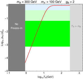
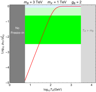
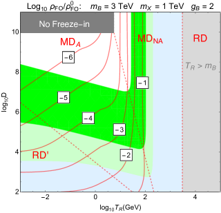
We show our results for the case of inflationary reheating in Fig. 12. The red curve gives the dilution factor as a function of over the range of where FI can occur, with the two panels corresponding to the two cases of Eq. (67). The shaded regions denote the associated collider signal for the chosen masses and for the value of on the red curve, as found in Fig. 6.
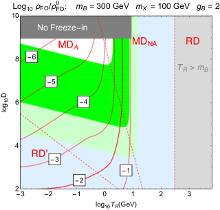
Next we consider the more general case of both and , with results in Fig. 13 for the same choices of and masses. The contours of both panels show that the FO contribution is always reduced as either is reduced or is increased. The shaded regions of both panels refer to the FI contribution, and are taken from the appropriate panels of Figs. 8 and 9. In the green regions, where FI gives displaced vertices, the FO contribution is suppressed by 1 to 6 orders of magnitude compared to conventional FO during the RD era, and hence is typically expected to be negligible.
In the right panel of Fig. 13, the three dashed red lines separate the regions where FO occurs, from right to left, in the (RD, MDNA, MDA, RD′) eras. These three boundaries, from right to left, correspond to FO temperatures of and . The FO abundance in region is
| (68) |
which can be compared to the FI result of Eq. (31) and gives the asymptotic slopes of the contours in both panels of Figs. 12 and 13.
References
- [1] S. Hannestad, Phys. Rev. D 70, 043506 (2004) [astro-ph/0403291]; F. De Bernardis, Nucl. Phys. Proc. Suppl. 194, 39 (2009).
- [2] M. Kawasaki, K. Kohri and N. Sugiyama, Phys. Rev. D 62, 023506 (2000) [astro-ph/0002127]; K. Ichikawa, M. Kawasaki and F. Takahashi, Phys. Rev. D 72, 043522 (2005) [astro-ph/0505395].
- [3] J. McDonald, Phys. Rev. D 43, 1063 (1991).
- [4] D. J. H. Chung, E. W. Kolb and A. Riotto, Phys. Rev. D 60, 063504 (1999) [hep-ph/9809453].
- [5] G. F. Giudice, E. W. Kolb and A. Riotto, Phys. Rev. D 64, 023508 (2001) [hep-ph/0005123].
- [6] M. Kamionkowski and M. S. Turner, Phys. Rev. D 42, 3310 (1990).
- [7] L. J. Hall, K. Jedamzik, J. March-Russell and S. M. West, JHEP 1003, 080 (2010) [arXiv:0911.1120 [hep-ph]].
- [8] T. Moroi and L. Randall, Nucl. Phys. B 570, 455 (2000) [hep-ph/9906527]; R. Allahverdi and M. Drees, Phys. Rev. Lett. 89, 091302 (2002) [hep-ph/0203118]; R. Allahverdi and M. Drees, Phys. Rev. D 66, 063513 (2002) [hep-ph/0205246]. B. S. Acharya, G. Kane, S. Watson and P. Kumar, Phys. Rev. D 80, 083529 (2009) [arXiv:0908.2430].
- [9] A. Monteux and C. S. Shin, arXiv:1505.03149 [hep-ph].
- [10] C. Cheung, G. Elor, L. J. Hall and P. Kumar, JHEP 1103, 042 (2011) [arXiv:1010.0022].
- [11] S. Chatrchyan et al. [CMS Collaboration], JHEP 1302, 085 (2013) [arXiv:1211.2472 [hep-ex]].
- [12] G. Aad et al. [ATLAS Collaboration], arXiv:1504.05162 [hep-ex].
- [13] V. Khachatryan et al. [CMS Collaboration], Phys. Rev. D 91, no. 1, 012007 (2015) [arXiv:1411.6530 [hep-ex]].
- [14] G. Aad et al. [ATLAS Collaboration], arXiv:1504.03634 [hep-ex].
- [15] G. Aad et al. [ATLAS Collaboration], JHEP 1411, 088 (2014) [arXiv:1409.0746 [hep-ex]].
- [16] V. Khachatryan et al. [CMS Collaboration], Phys. Rev. D 91, no. 5, 052012 (2015) [arXiv:1411.6977 [hep-ex]].
- [17] G. Aad et al. [ATLAS Collaboration], Phys. Rev. D 88, no. 11, 112003 (2013) [arXiv:1310.6584 [hep-ex]].
- [18] V. Khachatryan et al. [CMS Collaboration], Eur. Phys. J. C 75, no. 4, 151 (2015) [arXiv:1501.05603 [hep-ex]].
- [19] S. Dimopoulos and L. J. Hall, Phys. Lett. B 196, 135 (1987).
- [20] J. E. Kim and H. P. Nilles, Phys. Lett. B 138, 150 (1984).
- [21] B. Bellazzini, C. Csaki, J. Hubisz, J. Shao and P. Tanedo, JHEP 1109, 035 (2011) [arXiv:1106.2162 [hep-ph]].
- [22] K. Rajagopal, M. S. Turner and F. Wilczek, Nucl. Phys. B 358, 447 (1991).
- [23] L. Covi, J. E. Kim and L. Roszkowski, Phys. Rev. Lett. 82, 4180 (1999) [hep-ph/9905212].
- [24] L. Covi, H. B. Kim, J. E. Kim and L. Roszkowski, JHEP 0105, 033 (2001) [hep-ph/0101009].
- [25] E. J. Chun, Phys. Rev. D 84, 043509 (2011) [arXiv:1104.2219 [hep-ph]].
- [26] A. Strumia, JHEP 1006, 036 (2010) [arXiv:1003.5847 [hep-ph]].
- [27] K. J. Bae, K. Choi and S. H. Im, JHEP 1108, 065 (2011) [arXiv:1106.2452 [hep-ph]].
- [28] K. Tamvakis and D. Wyler, Phys. Lett. B 112, 451 (1982).
- [29] C. Cheung, G. Elor and L. J. Hall, Phys. Rev. D 85, 015008 (2012) [arXiv:1104.0692 [hep-ph]].
- [30] P. Moxhay and K. Yamamoto, Phys. Lett. B 151, 363 (1985).
- [31] M. P. Hertzberg, M. Tegmark and F. Wilczek, Phys. Rev. D 78, 083507 (2008) [arXiv:0807.1726 [astro-ph]].
- [32] F. D’Eramo, L. J. Hall and D. Pappadopulo, JHEP 1411, 108 (2014) [arXiv:1409.5123 [hep-ph]].
- [33] R. L. Davis, Phys. Lett. B 180, 225 (1986); C. Hagmann, S. Chang and P. Sikivie, Phys. Rev. D 63, 125018 (2001) [hep-ph/0012361]; T. Hiramatsu, M. Kawasaki, T. Sekiguchi, M. Yamaguchi and J. Yokoyama, Phys. Rev. D 83, 123531 (2011) [arXiv:1012.5502 [hep-ph]]; T. Hiramatsu, M. Kawasaki, K. Saikawa and T. Sekiguchi, Phys. Rev. D 85, 105020 (2012) [Erratum-ibid. D 86, 089902 (2012)] [arXiv:1202.5851 [hep-ph]].
- [34] K. A. Olive et al. [Particle Data Group Collaboration], Chin. Phys. C 38, 090001 (2014).
- [35] S. P. Martin, Phys. Rev. D 62, 095008 (2000) [hep-ph/0005116].
- [36] G. Barenboim, E. J. Chun, S. Jung and W. I. Park, Phys. Rev. D 90, no. 3, 035020 (2014) [arXiv:1407.1218 [hep-ph]].
- [37] A. Arvanitaki and A. A. Geraci, Phys. Rev. Lett. 113, no. 16, 161801 (2014) [arXiv:1403.1290 [hep-ph]].