DeepStereo: Learning to Predict New Views from the World’s Imagery

Abstract

Deep networks have recently enjoyed enormous success when applied to recognition and classification problems in computer vision [20, 29], but their use in graphics problems has been limited ([21, 7] are notable recent exceptions). In this work, we present a novel deep architecture that performs new view synthesis directly from pixels, trained from a large number of posed image sets. In contrast to traditional approaches which consist of multiple complex stages of processing, each of which require careful tuning and can fail in unexpected ways, our system is trained end-to-end. The pixels from neighboring views of a scene are presented to the network which then directly produces the pixels of the unseen view. The benefits of our approach include generality (we only require posed image sets and can easily apply our method to different domains), and high quality results on traditionally difficult scenes. We believe this is due to the end-to-end nature of our system which is able to plausibly generate pixels according to color, depth, and texture priors learnt automatically from the training data. To verify our method we show that it can convincingly reproduce known test views from nearby imagery. Additionally we show images rendered from novel viewpoints. To our knowledge, our work is the first to apply deep learning to the problem of new view synthesis from sets of real-world, natural imagery.

1 Introduction

(a)

(b)

Figure 1: The top image was synthesized from several input panoramas. A portion of two of the inputs is shown on the bottom row.
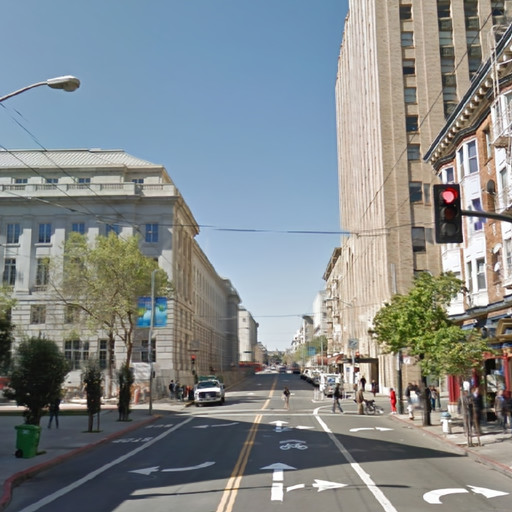
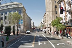
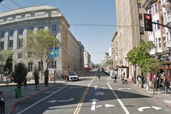
More results at: http://youtu.be/cizgVZ8rjKA

Estimating 3D shape from multiple posed images is a fundamental task in computer vision and graphics, both as an aid to image understanding and as a way to generate 3D representations of scenes that can be rendered and edited. In this work, we aim to solve the related problem of new view synthesis, a form of image-based rendering (IBR) where the goal is to synthesize a new view of a scene by warping and combining images from nearby posed images. This can be used for applications such as cinematography, virtual reality, teleconferencing [4], image stabilization [19], or 3-dimensionalizing monocular film footage.

New view synthesis is an extremely challenging, under-constrained problem. An exact solution would require full 3D knowledge of all visible geometry in the unseen view which is in general not available due to occluders. Additionally, visible surfaces may have ambiguous geometry due to a lack of texture. Therefore, good approaches to IBR typically require the use of strong priors to fill in pixels where the geometry is uncertain, or when the target color is unknown due to occlusions.

The majority of existing techniques for this problem involve traditional multi-view stereo and/or image warping methods and often explicitly model the stereo, color, and occlusion components of each target pixel [34, 1]. A key problem with these approaches is that they are prone to generating unrealistic and jarring rendering artifacts in the new view. Commonly seen artifacts include tearing around occluders, elimination of fine structures, and aliasing. Handling complex, self-occluding (but commonly seen) objects such as trees is particularly challenging for traditional approaches. Interpolating between wide baseline views tends to exacerbate these problems.

Deep networks have enjoyed huge success in recent years, particularly for image understanding tasks [20, 29]. Despite these successes, relatively little work exists on applying deep learning to computer graphics problems and especially to generating new views from real imagery. One possible reason is the perceived inability of deep networks to generate pixels directly, but recent work on denoising [35], super-resolution [6], and rendering [21] suggest that this is a misconception. Another common objection is that deep networks have a huge number of parameters and hence are prone to overfitting in the absence of enormous quantities of data, but recent work [29] has demonstrated state-of-the-art deep networks whose parameters number in the low millions, greatly reducing the potential for overfitting.

In this work we present a new approach to new view synthesis that uses deep networks to regress directly to output pixel colors given the posed input images. Our system is able to interpolate between views separated by a wide baseline and exhibits resilience to traditional failure modes, including graceful degradation in the presence of scene motion and specularities. We posit this is due to the end-to-end nature of the training, and the ability of deep networks to learn extremely complex non-linear functions of their inputs [25]. Our method makes minimal assumptions about the scene being rendered: largely, that the scene should be static and should exist within a finite range of depths. Even when these requirements are violated, the resulting images degrade gracefully and often remain visually plausible. When uncertainty cannot be avoided our method prefers to blur detail which generates much more visually pleasing results compared to tearing or repeating, especially when animated. Additionally, although we focus on its application to new view problems here, we believe that the deep architecture presented can be readily applied to other stereo and graphics problems given suitable training data.

For view synthesis, there is an abundance of readily available training data—any set of posed images can be used as a training set by leaving one image out and trying to reproduce it from the remaining images. We take that approach here, and train our models using large amounts of data mined from Google’s Street View, a massive collection of posed imagery spanning much of the globe [16]. Because of the variety of the scenes seen in training our system is robust and generalizes to indoor and outdoor imagery, as well as to image collections used in prior work.

We compare images generated by our model with the corresponding captured images on street and indoor scenes. Additionally, we compare our results qualitatively to existing state-of-the-art IBR methods.

2 Related Work

Learning depth from images. The problem of view synthesis is strongly related to the problem of predicting depth or 3D shape from imagery. In recent years, learning methods have been applied to this shape prediction problem, often from just a single image—a very challenging vision task. Automatic single-view methods include the Make3D system of Saxena et al. [26], which uses aligned photos and laser scans as training data, and the automatic photo pop-up work of Hoiem et al. [14], which uses images with manually annotated geometric classes. More recent methods have used Kinect data for training [15, 18] and deep learning methods for single view depth or surface normal prediction [9, 33]. However, the single-view problem remains very challenging. Moreover, gathering sufficient training data is difficult and time-consuming.

Other work has explored the use of machine learning for the stereo problem (i.e., using more than one frame). Learning has been used in several ways, including estimating the parameters of more traditional models such as MRFs [36] and learning low-level correlation filters for disparity estimation [24, 17].

Unlike this prior work, we learn to synthesize new views directly using a new deep architecture, and do not require known depth or disparity as training data.

View interpolation. There is a long history of work on image-based rendering in vision and graphics based on a variety of methods, including light fields [23, 13], image correspondence and warping [27], and explicit shape and appearance estimation [32, 37, 28]. Much of the recent work in this area has used a combination of 3D shape with image warping and blending [10, 12, 1, 2]. These methods are largely hand-built and do not leverage training data. Our goal is to learn a model for predicting new viewpoints by directly minimizing the prediction error on our training set.

We are particularly inspired by the work of Fitzgibbon et al. on IBR using image-based priors [11]. Like them, we consider the goal of faithfully reconstructing the actual output image to be the key problem to be optimized for, as opposed to reconstructing depth or other intermediate representations. We utilize state-of-the-art machine learning methods with a new architecture to achieve this goal. Szeliski [30] suggests using image prediction error as a metric for stereo algorithms; our method directly minimizes this prediction error.

Finally, a few recent papers have applied deep learning to synthesizing imagery. Dosovitskiy et al. train a network on synthetic images of rendered 3D chairs that can generate new chair images given parameters such as pose [7]. Kulkarni et al. propose a “deep convolutional inverse graphics network” that can parse and rerender imagery such as faces [22]. However, we believe ours is the first method to apply deep learning to synthesizing novel natural imagery from posed real-world input images.

3 Approach

Figure 2: The goal of image-based rendering is to render a new view at $C$ from existing images at $V_{1}$ and $V_{2}$.

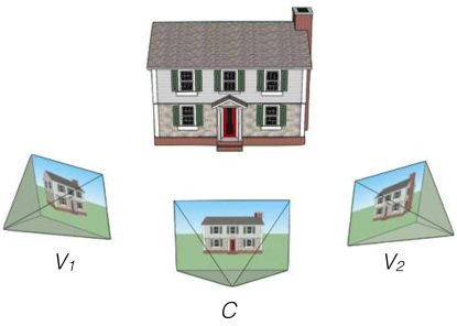
Given a set of posed input images $I_{1},I_{2},\dots,I_{n}$, with poses $V_{1},V_{2},\dots,V_{n}$, the view synthesis problem is to render a new image from the viewpoint of a new target camera $C$ (Fig. 2). Despite the representative power of deep networks, naively training a deep network to synthesize new views by supplying the input images $I_{k}$ as inputs directly is unlikely to work well, for two key reasons.

First, the pose parameters of $C$ and of the views $V_{1},V_{2},\dots,V_{n}$ would need to be supplied as inputs to the network in order to produce the desired view. The relationship between the pose parameters, the input pixels and the output pixels is complex and non-linear—the network would effectively need to learn how to interpret rotation angles and to perform image reprojection. Requiring the network to learn projection is inefficient—it is a straightforward operation that we can represent outside of the network.

Second, in order to synthesize a new view, the network would need to compare and combine potentially distant pixels in the original source images, necessitating very dense, long-range connections. Such a network would have many parameters and would be slow to train, prone to overfitting, and slow to run inference on. It is possible that a network structure could be designed to use the epipolar constraint internally in order to limit connections to those on corresponding epipolar lines. However, the epipolar lines, and thus the network connections, would be pose-dependent, making this very difficult and likely computationally inefficient in practice.

Using plane-sweep volumes. Instead, we address these problems by using ideas from traditional plane sweep stereo [3, 31]. We provide our network with a set of 3D plane sweep volumes as input. A plane sweep volume consists of a stack of images reprojected to the target camera $C$ (Fig. 3). Each image $I_{k}$ in the stack is reprojected into the target camera $C$ at a set of varying depths $d\in\{d_{1},d_{2},\dots d_{D}\}$ to form a plane sweep volume $V^{k}_{C}=\{P^{k}_{1},P^{k}_{2},\dots P^{k}_{D}\}$, where $P^{k}_{i}$ refers to the reprojected image $I_{k}$ at depth $d_{i}$. Reprojecting an input image into the target camera only requires basic texture mapping capabilities and can be performed on a GPU. A separate plane sweep volume $V^{k}_{C}$ is created for each input image $I_{k}$. Each voxel $v^{k}_{i,j,z}$ in each plane sweep volume $V^{k}_{C}$ has $R$, $G$, $B$ and $A$ (alpha) components. The alpha channel indicates the availability of source pixels for that voxel (e.g., alpha is zero for pixels outside the field of view of a source image).

Figure 3: Plane sweep stereo reprojects images $I_{1}$ and $I_{2}$ from viewpoints $V_{1}$ and $V_{2}$ to the target camera $C$ at a range of depths $d\in{d_{1}\dots d_{D}}$. The dotted rays indicate the pixels from the input images reprojected to a particular output image pixel, and the images above each input view show the corresponding reprojected images at different depths.

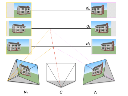
Using plane sweep volumes as input to the network removes the need to supply the pose parameters since they are now implicit inputs used in the construction of the plane sweep volume. Additionally, the epipolar constraint is trivially enforced within a plane sweep volume: corresponding pixels are now in corresponding $i,j$ columns of the plane sweep volumes. Thus, long range connections between pixels are no longer needed, so a given output pixel depends only on a small column of voxels from each of the per-source plane sweep volumes. Similarly, the computation performed to produce an output pixel $p$ at location $i,j$ should be largely independent of the pixel location. This allows us to use more efficient convolutional neural networks. Our model applies 2D convolutional layers to each plane within the input plane sweep volume. In addition to sharing weights within convolutional layers we make extensive use of weight sharing across planes in the plane sweep volume. Intuitively, weight sharing across planes make sense since the computation to be performed on each plane will be largely independent of the plane’s depth.

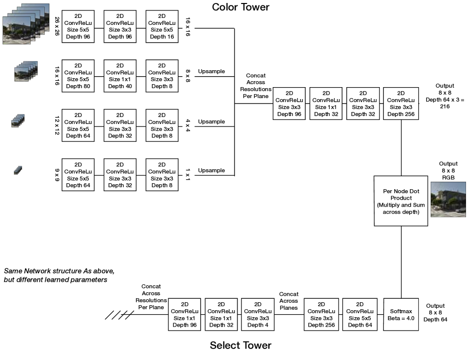
Our model. Our network architecture (Fig. 4) consists of two towers of layers, a selection tower and a color tower. The intuition behind this dual network architecture is that there are there are really two related tasks that we are trying to accomplish:

• Depth prediction. First, we want to know the approximate depth for each pixel in the output image. This enables us to determine the source image pixels we should use to generate that output pixel. In prior work, this kind of probability over depth might be computed via SSD, NCC, or variance; we learn how to compute these probabilities using training data.

• Color prediction. Second, we want to produce a color for that output pixel, given all of the relevant source image pixels. Again, the network does not just perform, e.g., a simple average, but learns how to optimally combine the source image pixels from training data.

The two towers in our network correspond to these two tasks: the selection tower produces a probability map (or “selection map”) for each depth indicating the likelihood of each pixel having a given depth. The color tower produces a full color output image for each depth; one can think of this tower as producing the best color it can for each depth, assuming that the depth is the correct one. These $D$ color images are then combined by computing a per-pixel weighted sum with weights drawn from the selection maps—the selection maps decide on the best color layers to use for each output pixel. This simple new approach to view synthesis has several attractive properties. For instance, we can learn all of the parameters of both towers simultaneously, end-to-end using deep learning methods. The weighted averaging across color layers also yields some resilience to uncertainty—regions where the algorithm is not confident tend to be blurred out, rather than being filled with warped or distorted input pixels.

Figure 4: The basic architecture of our network, with selection and color towers. The final output image is produced by element-wise multiplication of the selection and color tower outputs and then computing the sum over the depth planes. Fig. 7 shows the full complete network details.

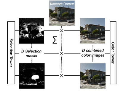
More formally, the selection tower computes, for each pixel $p_{i,j}$, in each plane $P_{z}$, the selection probability $s_{i,j,z}$ for the pixel being at that depth. The color tower computes for each pixel $p_{i,j}$ in each plane $P_{z}$ the color $c_{i,j,z}$ for the pixel at that plane. The final output color for each pixel is computed as a weighted summation over the output color planes, weighted by the selection probability (Fig. 4):

$$c^{f}_{i,j}=\sum s_{i,j,z}\times c_{i,j,z}.$$ (1)

The input to each tower is the set of plane sweep volumes $V^{k}_{C}$. The first layer of both towers concatenates the input plane sweep volumes over the source. This allows the networks to compare and combine reprojected pixel values across sources. We now describe the computation performed in each tower in more detail.

Figure 5: The selection tower learns to produce a selection probability $s_{i,j,z}$ for each pixel $p_{i,j}$ in each depth plane $P_{z}$.

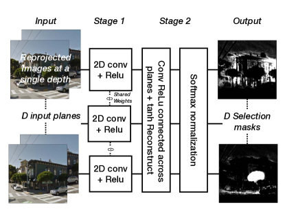
The selection tower. The selection tower consists of two main stages. The first stage is a number of $2D$ convolutional rectified linear layers that share weights across all planes. Intuitively the early layers will compute features that are independent of depth, such as pixel differences, so their weights can be shared. The second stage of layers are connected across depth planes, in order to model interactions between depth planes such as those caused by occlusion (e.g., the network might learn to prefer closer planes that have high scores in case of ambiguities in depth). The final layer of the network is a per-pixel softmax normalization transformer over depth. The softmax transformer encourages the model to pick a single depth plane per pixel, whilst ensuring that the sum over all depth planes is 1. We found that using a $\tanh$ activation for the penultimate layer gives more stable training than the more natural choice of a linear layer. In our experiments the linear layer would often “shut down” certain depth planes and never recover, presumably, due to large gradients from the softmax layer. The output of the selection tower is a 3D volume of single-channel nodes $s_{i,j,z}$ where

$$\sum_{z=1}^{D}s_{i,j,z}=1.$$

Figure 6: The color tower learns to combine and warp pixels across sources to produce a color $c_{i,j,z}$ for each pixel $p_{i,j}$ in each depth plane $P_{z}$.

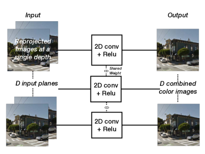
The color tower. The color tower (Fig. 6) is simpler and consists of only 2D convolutional rectified linear layers that share weights across all planes, followed by a linear reconstruction layer. Occlusion effects are not relevant for the color layer so no across-depth interaction is needed. The output of the color tower is again a 3D volume of nodes $c_{i,j,z}$. Each node in the output has 3 channels, corresponding to $R$, $G$ and $B$.

The output of the color tower and the selection tower are multiplied together per node to produce the output image $c^{f}$ (Eq. 1). During training the resulting image is compared with the known target image $I^{t}$ using a per-pixel $L_{1}$ loss. The total loss is thus:

$$L=\sum_{i,j}|c^{t}_{i,j}-c^{f}_{i,j}|$$

where $c^{t}_{i,j}$ is the target color at pixel $i,j$.

Multi-resolution patches. Rather than predict a full image at a time, we predict the output image patch-by-patch. We found that passing in a set of lower resolution versions of successively larger areas around the input patches helped improve results by providing the network with more context. We pass in four different resolutions. Each resolution is first processed independently by several layers and then upsampled and concatenated before entering the final layers. The upsampling is performed using nearest neighbor interpolation.

The full details of the complete network are shown in Fig. 7.

Figure 7: The full network diagram. The initial stages of both the color and select towers are the same structure, but do not share parameters.

3.1 Training

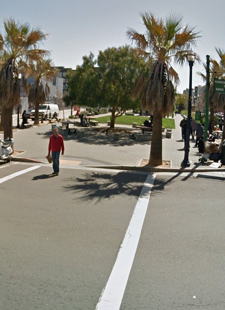
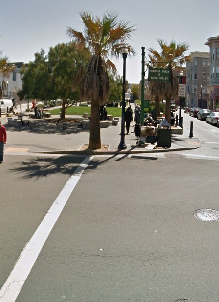
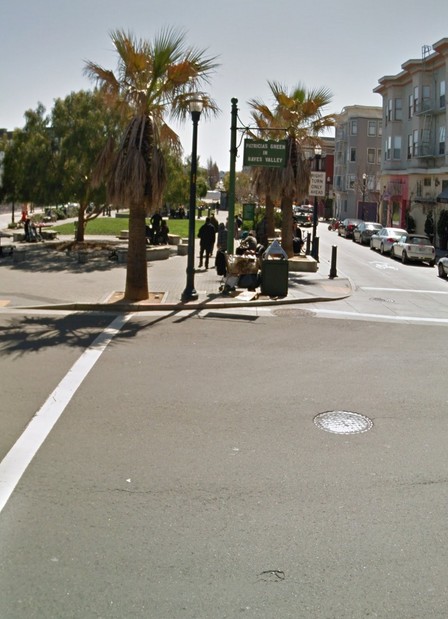
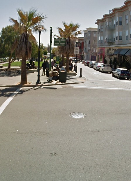
To train our network, we used images of street scenes captured by a moving vehicle. The images were posed using a combination of odometry and traditional structure-from-motion techniques [16]. The vehicle captures a set of images, known as a rosette, from different directions for each exposure. The capturing camera uses a rolling shutter sensor, which is taken into account by our camera model. We used approximately 100K of such image sets during training.

We used a continuously running online sample generation pipeline that selected and reprojected random patches from the training imagery. The network was trained to produce $8\times 8$ patches from overlapping input patches of size $26\times 26$. We used 96 depth planes in all results shown. Since the network is fully convolutional there are no border effects as we transition between patches in the output image. In order to increase the variability of the patches that the network sees during training patches from many images are mixed together to create mini-batches of size 400. We trained our network with Adagrad [8] with an initial learning rate of 0.0005 using the system described by Dean, et al. [5]. In our experiments, training converged after approximately 1M steps. Due to sample randomization, it is unlikely that any patch was used more than once in training. Thanks to our large volume of training data, training data augmentation was not required. We selected our training data by first randomly selecting two rosettes that were captured relatively close together, within 30cm, we then found other nearby rosettes that were spaced up to 3m away. We select one of the images in the center rosette as the target and train to produce it from the others.

4 Results

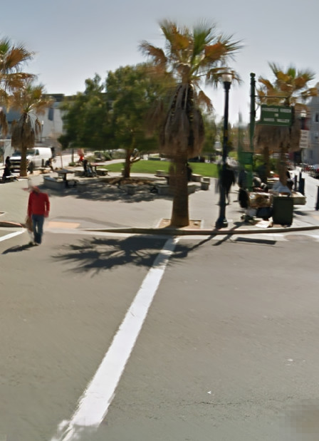
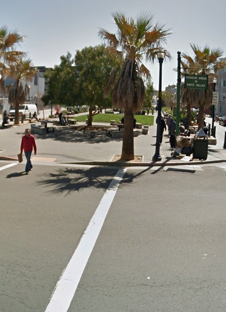
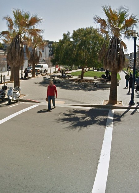
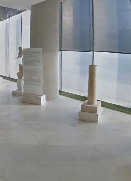
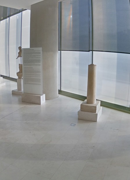
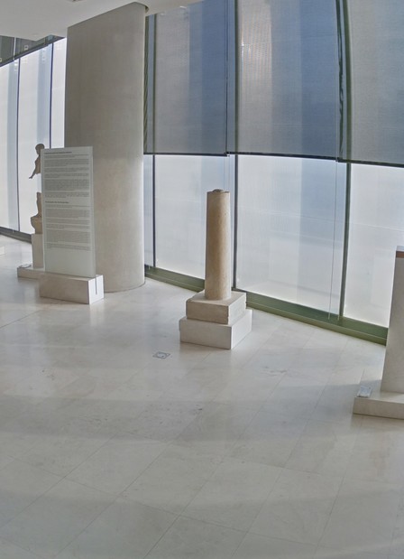
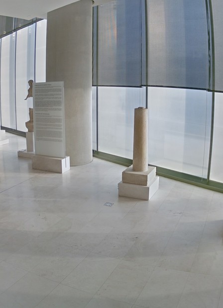
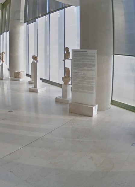
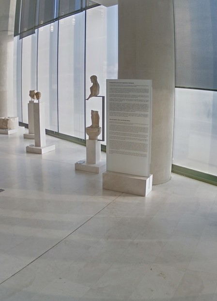
To evaluate our model on view interpolation, we generated a novel image from the same viewpoint as a known (but withheld) image captured by the Street View camera. Representative results for an outdoor scene are shown in Figure 8, and for an indoor scene in Figure 9. We also used our model to interpolate from image data featured in the work of Chaurasia, et al. [2, 1], as shown in Figure 10. The imagery from this prior work is quite different from our training images, as these prior images were taken with a handheld DSLR camera. Despite the fact that our model was not trained directly for this task, it did a reasonable job at reproducing the input imagery and at interpolating between them.

These images were rendered in small patches, as rendering an entire image would be prohibitively expensive in RAM. It takes about 12 minutes on a multi-core workstation to render a $512\times 512$ pixel image. However, our current implementation does not fully exploit the convolutional nature of our model, so these times could likely be reduced to minutes or even seconds by a GPU implementation in the spirit of Krizhevsky, et al. [20].

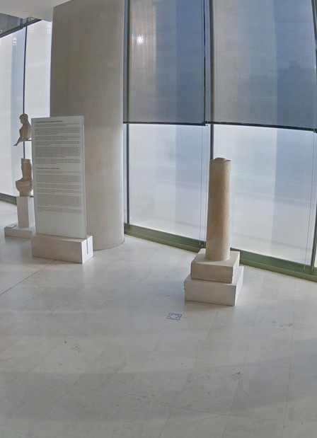
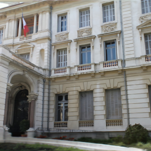
Overall, our model produces plausible outputs that are difficult to immediately distinguish from the original imagery. The model can handle a variety of traditionally difficult surfaces, including trees and glass as shown in Figure 1. Although the network does not attempt to model specular surfaces, the results show graceful degradation in their presence, as shown in Figure 9 as well as the supplemental video.

As the above figures demonstrate, our model does well at interpolating Street View data and is competitive on the dataset from [1], even though our method was trained on data which has different /characteristics from the imagery and cameras in this prior dataset. Noticeable artifacts in our results include a slight loss of resolution and the disappearance of thin foreground structures. Additionally, partially occluded objects tend to appear overblurred in the output image. Finally, our model is unable to render surfaces that appear in none of the inputs.

Moving objects, which occur often in the training data, are handled gracefully by our model: They appear blurred in a manner that evokes motion blur (e.g. see pedestrians in Figure 8). On the other hand, violating the maximum camera motion assumption significantly degrades the quality of the interpolated results.

(a) Our result.

(b) Reference image.

(c) Crops of the five input panoramas.

Figure 8: San Francisco park.

(a) Our result.

(b) Reference image.

(c) Crops of the five input panoramas.

Figure 9: Acropolis Museum.

(a) Our result.

(b) Reference image.

Figure 10: Our method applied to images from [1].

5 Discussion

We have shown that it is possible to train a deep network end-to-end to perform novel view synthesis. Our method is general and requires only sets of posed imagery. Results comparing real views with synthesized views show the generality of our method. Our results are competitive with existing image-based rendering methods, even though our training data is considerably different than the test sets.

The two main drawbacks of our method are speed and inflexibility in the number of input images. We have not optimized our network for execution time but even with optimizations it is likely that the current network is far from real time. Our method currently requires reprojecting each input image to a set of depth planes; we currently use 96 depth planes, which limits the resolution of the output images that we can produce. Increasing the resolution would require a larger number of depth planes, which would mean that the network takes longer to train, uses more RAM and takes longer to run. This is a drawback shared with other volumetric stereo methods; however, our method requires reprojected images per rendered frame, rather than just once when creating the scene. We plan to explore pre-computing parts of the network and warping to new views before running the final layers.

Another interesting direction of future work is to explore different network architectures. For instance, one could use recurrent networks to process the reprojected depth images one depth at a time. A recurrent network would not have connections across depth, and so would likely be faster to run inference on. We believe that with some of these improvements our method has the potential to offer real-time performance on a GPU.

Our network is trained using 5 input views per target view. We currently can’t change the number of input views after training which is non-optimal when there are denser sets of cameras that can be exploited, as in the sequences from [1]. One idea is to choose the set of input views per pixel; however, this risks introducing discontinuties at transitions between chosen views. Alternatively, it is possible that a more complex recurrent model could handle arbitrary numbers of input views, though this would likely complicate training. It would also be interesting to explore the outputs of the intermediate network layers of the network. For instance, it is likely that the network learns a strong pixel similarity measure in the select tower. These could be incorporated into a more traditional stereo framework.

Finally, a similar network could likely be applied to the problem of synthesizing intermediate frames in video, as well as for regressing to a depth map, given appropriate training data.

References

- [1] G. Chaurasia, S. Duchêne, O. Sorkine-Hornung, and G. Drettakis. Depth synthesis and local warps for plausible image-based navigation. ACM Transactions on Graphics, 32, 2013.
- [2] G. Chaurasia, O. Sorkine, and G. Drettakis. Silhouette-aware warping for image-based rendering. Computer Graphics Forum (Proc. EGSR), 30(4), 2011.
- [3] R. T. Collins. A space-sweep approach to true multi-image matching. In CVPR, 1996.
- [4] A. Criminisi, A. Blake, C. Rother, J. Shotton, and P. Torr. Efficient dense stereo with occlusions for new view-synthesis by four-state dynamic programming. 2007.
- [5] J. Dean, G. Corrado, R. Monga, K. Chen, M. Devin, M. Mao, M. Ranzato, A. Senior, P. Tucker, K. Yang, Q. V. Le, and A. Y. Ng. Large scale distributed deep networks. In P. Bartlett, F. Pereira, C. Burges, L. Bottou, and K. Weinberger, editors, NIPS, pages 1232–1240. 2012.
- [6] C. Dong, C. C. Loy, K. He, and X. Tang. Learning a deep convolutional network for image super-resolution. In ECCV. 2014.
- [7] A. Dosovitskiy, J. Springenberg, and T. Brox. Learning to generate chairs with convolutional neural networks. In CVPR, 2015.
- [8] J. Duchi, E. Hazan, and Y. Singer. Adaptive subgradient methods for online learning and stochastic optimization. Technical Report UCB/EECS-2010-24, EECS Department, University of California, Berkeley, Mar 2010.
- [9] D. Eigen, C. Puhrsch, and R. Fergus. Depth map prediction from a single image using a multi-scale deep network. In Advances in neural information processing systems, 2014.
- [10] M. Eisemann, B. De Decker, M. Magnor, P. Bekaert, E. de Aguiar, N. Ahmed, C. Theobalt, and A. Sellent. Floating textures. Computer Graphics Forum (Proc. of Eurographics EG), 27(2):409–418, Apr. 2008. Received the Best Student Paper Award at Eurographics 2008.
- [11] A. Fitzgibbon, Y. Wexler, and A. Zisserman. Image-based rendering using image-based priors. In ICCV, 2003.
- [12] M. Goesele, J. Ackermann, S. Fuhrmann, C. Haubold, R. Klowsky, D. Steedly, and R. Szeliski. Ambient point clouds for view interpolation. In SIGGRAPH, 2010.
- [13] S. J. Gortler, R. Grzeszczuk, R. Szeliski, and M. F. Cohen. The lumigraph. In SIGGRAPH, 1996.
- [14] D. Hoiem, A. A. Efros, and M. Hebert. Automatic photo pop-up. In SIGGRAPH, 2005.
- [15] K. Karsch, C. Liu, and S. B. Kang. DepthTransfer: Depth extraction from video using non-parametric sampling. IEEE Trans. on Pattern Analysis and Machine Intelligence, 2014.
- [16] B. Klingner, D. Martin, and J. Roseborough. Street view motion-from-structure-from-motion. In The IEEE International Conference on Computer Vision (ICCV), December 2013.
- [17] K. R. Konda and R. Memisevic. Unsupervised learning of depth and motion. CoRR, abs/1312.3429, 2013.
- [18] J. Konrad, M. Wang, and P. Ishwar. 2d-to-3d image conversion by learning depth from examples. In CVPR Workshops, 2012.
- [19] J. Kopf, M. F. Cohen, and R. Szeliski. First-person hyper-lapse videos. In SIGGRAPH, 2014.
- [20] A. Krizhevsky, I. Sutskever, and G. Hinton. Imagenet classification with deep convolutional neural networks. In Advances in neural information processing systems, 2012.
- [21] T. Kulkarni, W. Whitney, K. Pushmeet, and J. Tenenbaum. Deep convolutional inverse graphics network. arXiv preprint arXiv:1503.03167, 2015.
- [22] T. D. Kulkarni, W. Whitney, P. Kohli, and J. B. Tenenbaum. Deep convolutional inverse graphics network. CoRR, abs/1503.03167, 2015.
- [23] M. Levoy and P. Hanrahan. Light field rendering. In SIGGRAPH, 1996.
- [24] R. Memisevic and C. Conrad. Stereopsis via deep learning. In NIPS workshop on Deep Learning and Unsupervised Feature Learning, 2011.
- [25] G. Montufar, R. Pascanu, K. Cho, and Y. Bengio. On the number of linear regions of deep neural networks. In Advances in neural information processing systems, 2014.
- [26] A. Saxena, M. Sun, and A. Y. Ng. Make3d: Learning 3d scene structure from a single still image. IEEE Trans. on Pattern Analysis and Machine Intelligence, 31(5), May 2009.
- [27] S. M. Seitz and C. R. Dyer. View morphing. In SIGGRAPH, 1996.
- [28] Q. Shan, R. Adams, B. Curless, Y. Furukawa, and S. M. Seitz. The visual turing test for scene reconstruction. In Proc. 3D Vision, 2013.
- [29] C. Szegedy, W. Liu, Y. Jia, P. Sermanet, S. Reed, D. Anguelov, D. Erhan, V. Vanhoucke, and A. Rabinovich. Going deeper with convolutions. In CVPR, 2015.
- [30] R. Szeliski. Prediction error as a quality metric for motion and stereo. In Proceedings of the International Conference on Computer Vision-Volume 2 - Volume 2, ICCV ’99, pages 781–, Washington, DC, USA, 1999. IEEE Computer Society.
- [31] R. Szeliski and P. Golland. Stereo matching with transparency and matting. IJCV, 32(1), 1999.
- [32] S. Vedula, P. Rander, R. Collins, and T. Kanade. Three-dimensional scene flow. IEEE Trans. on Pattern Analysis and Machine Intelligence, 27(3), March 2005.
- [33] X. Wang, D. F. Fouhey, and A. Gupta. Designing deep networks for surface normal estimation. CoRR, abs/1411.4958, 2014.
- [34] O. Woodford, I. Reid, P. Torr, and A. Fitzgibbon. On new view synthesis using multiview stereo. 2007.
- [35] J. Xie, L. Xu, and E. Chen. Image denoising and inpainting with deep neural networks. In Advances in neural information processing systems, 2012.
- [36] K. Yamaguchi, T. Hazan, D. A. McAllester, and R. Urtasun. Continuous markov random fields for robust stereo estimation. CoRR, abs/1204.1393, 2012.
- [37] C. L. Zitnick, S. B. Kang, M. Uyttendaele, S. Winder, and R. Szeliski. High-quality video view interpolation using a layered representation. In SIGGRAPH, 2004.