\titlealternative

Systemic risk in multiplex networks with asymmetric coupling and threshold feedback \authoralternativeR. Burkholz, M.V. Leduc, A. Garas & F. Schweitzer

References

Rebekka Burkholz    Matt V. Leduc    Antonios Garas & Frank Schweitzer Chair of Systems Design, ETH Zurich, Weinbergstrasse 58, 8092 Zurich, Switzerland

Systemic risk in multiplex networks
with asymmetric coupling and threshold feedback

Rebekka Burkholz    Matt V. Leduc    Antonios Garas & Frank Schweitzer Chair of Systems Design, ETH Zurich, Weinbergstrasse 58, 8092 Zurich, Switzerland
Abstract

We study cascades on a two-layer multiplex network, with asymmetric feedback that depends on the coupling strength between the layers. Based on an analytical branching process approximation, we calculate the systemic risk measured by the final fraction of failed nodes on a reference layer. The results are compared with the case of a single layer network that is an aggregated representation of the two layers. We find that systemic risk in the two-layer network is smaller than in the aggregated one only if the coupling strength between the two layers is small. Above a critical coupling strength, systemic risk is increased because of the mutual amplification of cascades in the two layers. We even observe sharp phase transitions in the cascade size that are less pronounced on the aggregated layer. Our insights can be applied to a scenario where firms decide whether they want to split their business into a less risky core business and a more risky subsidiary business. In most cases, this may lead to a drastic increase of systemic risk, which is underestimated in an aggregated approach.

  • (4)
  • (5)
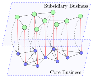
  • (6)
  • 1 Introduction

  • (7) Cascading failures in complex systems can be understood as a process by which the initial failure of a small set of individual components leads to the failure a significant fraction of the system’s components. This is due to interconnections between the different components of the system. Such a phenomenon can occur in physical systems such as power grids (e.g. Carreras2004, Kinney2005 and Brummitt2012), but also in complex organizations like interbank systems (e.g. EisenbergNoe2001, Gai2010, Battiston2012a and Amini2010). A general framework to study such cascading failures in networked systems was developed in Lorenz2009b, and extended recently to work in more general topologies in Burkholz2015.
  • (8) In many situations, cascading failures can be influenced by the combination of different types of interactions between the individual components of the system. This is the case in interbank systems, where banks are exposed to each other via different types of financial obligations (loans, derivative contracts, etc.) (e.g. KapadiaMay2012 and MontagnaKok2013). The bankruptcy of a bank can thus cascade to other banks in non-standard ways. Another example are firms diversifying their activities across different business units, each of which is exposed to cascade risk in its own field of activity.
  • (9) An important question we wish to investigate in this article is how diversification across different types of interactions can affect the risk of cascading failures. For that purpose, we study the case of a firm that diversifies its activities across a core-business unit and a subsidiary-business unit. Each business unit is exposed to other firms’ business units in the same sector of business activity (either core or subsidiary). This means that a business unit can fail (i.e. go bankrupt) as a result of a cascade of failures (i.e. bankruptcies) in the same sector of business activity.
  • (10) The question of the structuring of a firm into sub-units has been studied from a different angle in the financial economics literature (e.g. Lewellen1971 and MaksimovicPhillips2002) and often focuses on the efficiency of the allocation of its resources across different industries. Another question that has received some attention is that of whether a firm can diversify the risk of its income streams by operating in different business areas. Namely, LevySarnat1970, SmithSchreiner1969 and AmihudLev1981 studied how conglomerates can diversify the risk associated with their revenue streams from the perspective of portfolio theory.
  • (11) Here, we use a complex networks approach and we view the system of firm activities as an interconnected multi-layered network (see gao2012; DAgostino2014; kivela2014; Garas2015). The distinct layers of this network contain individual networks defined by a particular type of interactions according to a given business activity, while the inter-connections between layers allow for cross-layer interactions. In this setting we develop a model where failures (i.e. bankruptcies) on two different network layers affect firms asymmetrically: The first layer represents exposures between the firms in the core business while the second layer represents exposures between firms in the subsidiary business. Failure (i.e. bankruptcy) of a firm’s core business unit implies failure of its subsidiary business unit, whereas failure of a firm’s subsidiary business unit only causes a shock to the firm’s resistance threshold in its core business unit (see Fig. 1 for an illustration). We find that when the coupling strength from the core to the subsidiary layer is varied only slightly, there is a sharp transition between a safe regime, where there is no cascade of failures, and a catastrophic regime, where there is a full cascade of failures. Moreover, when comparing the two-layer network to the single-layer network formed by aggregating the two layers, we find that cascades can be larger on the two-layer network than on the aggregated one. On the other hand, by varying the strength of the feedback between the two layers, we identify the existence of a regime where the two-layer network is safer than the aggregated one and another regime where the reverse holds. This points to the critical importance of the coupling of the layers when structuring a firm into different business units. Also, dealing with aggregated network data that ignores the fine structure of the coupling between different layers can lead to significant underestimation or overestimation of cascade risk.
  • (12) The article is structured as follows. In Section 2, we describe the two-layer cascade model. In Section 3, we derive a branching process approximation as an approximation for large networks and use it to analyze the aforementioned phenomena. These phenomena are presented in Section 4 where we compare our analytical results with simulations and analyse further the observed phase transitions. In Section 5, we conclude and interpret the consequences of our theoretical investigations for the application to networks of firms that might decide about merging their core and their subsidiary business.
  • (13)
  • Refer to caption
    Figure 1: Illustration of a system with asymmetrically coupled layers. A failure (or bankruptcy) on the Core Business layer implies a failure on the Subsidiary Business layer. This coupling is illustrated by an inter-layer dependency link (red arrow). On the other hand, a failure on the Subsidiary Business layer only decreases a node’s failure threshold on the Core Business layer. This coupling is illustrated using dashed black arrows. The intra-layer links represent business relations or other forms of interactions due to normal business.
  • (14)
  • (15)
  • 2 Model

  • (16) We first consider a finite model with N𝑁N firms. Each firm can be represented by a node i𝑖i present on each of two different layers: layer 00 (the core-business layer) and layer 111 (the subsidiary-business layer). Each layer l{0,1}𝑙01l\in\{0,1\} has a topology represented by an adjacency matrix Glsubscript𝐺𝑙G_{l}. On each layer l𝑙l, node i𝑖i can be in one of two states sli{0,1}subscriptsuperscript𝑠𝑖𝑙01s^{i}_{l}\in\{0,1\}, healthy (sli=0subscriptsuperscript𝑠𝑖𝑙0s^{i}_{l}=0) or failed (sli=1subscriptsuperscript𝑠𝑖𝑙1s^{i}_{l}=1). s0i=1subscriptsuperscript𝑠𝑖01s^{i}_{0}=1 represents the bankruptcy of firm i𝑖i’s core-business unit, whereas s1i=1subscriptsuperscript𝑠𝑖11s^{i}_{1}=1 represents the bankruptcy of its subsidiary-business unit. This state is determined by two other variables: a node’s fragility on a given layer ϕlisubscriptsuperscriptitalic-ϕ𝑖𝑙\phi^{i}_{l}, which accumulates the load a node carries, and its threshold θlisubscriptsuperscript𝜃𝑖𝑙\theta^{i}_{l} on that layer, which determines the amount of load it can carry without failing. Whenever the fragility exceeds the threshold ϕliθlisubscriptsuperscriptitalic-ϕ𝑖𝑙subscriptsuperscript𝜃𝑖𝑙\phi^{i}_{l}\geq\theta^{i}_{l}, the node fails on that layer and cannot recover at a later point in time.
  • (17) On each layer, we assume that a cascade of failures spreads according to the threshold failure mechanism of Watts2002SimpleModelof. Thus a node fails if a sufficient fraction of its neighbors have failed. The fragility of a node i𝑖i of degree klsubscript𝑘𝑙k_{l} on layer l𝑙l (i.e. a node with klsubscript𝑘𝑙k_{l} neighbors on layer l𝑙l) can be expressed as
  • (18)
    ϕli(kl)=1kljnbl(i)slj=nlklsuperscriptsubscriptitalic-ϕ𝑙𝑖subscript𝑘𝑙1subscript𝑘𝑙subscript𝑗subscriptnblisuperscriptsubscript𝑠𝑙𝑗subscript𝑛𝑙subscript𝑘𝑙\phi_{l}^{i}(k_{l})=\frac{1}{k_{l}}\sum_{j\in\rm{nb_{l}}(i)}s_{l}^{j}=\frac{n_{l}}{k_{l}} (1)
    where nbl(i)subscriptnbli\rm{nb_{l}}(i) is the set of nodes in i𝑖i’s neighborhood on layer l𝑙l and nlsubscript𝑛𝑙n_{l} is the number of failed neighbors on layer l𝑙l. This failure mechanism is useful to model a firm diversifying its exposure to failure risk across neighbors: the more neighbors a node has, the less it is exposed to the failure of a single neighbor. A cascade of failures thus starts with an initial fraction of failed nodes. These failures can then spread to their neighbors in discrete time steps. The load ϕlisuperscriptsubscriptitalic-ϕ𝑙𝑖\phi_{l}^{i} of a node i𝑖i is thus updated at each time step t𝑡t. This model has been studied extensively on single-layer networks, in the context of configuration model type random graphs with a given degree distribution (Gleeson2007; Dodds2009; Payne2009; Amini2010; Tessone2012) or trees (Hurd2013), and has been adapted to financial networks of interbank lending (Gai2010; Battiston2012a; Roukny2013). In Burkholz2015 a mesoscopic perspective is added by studying conditional failure probabilities given the degree of node. Generalizations of the model to weighted networks can be found in Amini2010; Hurd2013 and Burkholz2015.
  • (19) We extend Watts’ model to a multiplex setting with non-symmetric dependence between the layers. The two network layers are related by partial dependency links (see Fig. 1). These are directed links connecting a node on layer 00 to its alter ego on layer 111. These links are characterized by weights r01,r10[0,1]subscript𝑟01subscript𝑟1001r_{01},\ r_{10}\in[0,1] affecting the size of a shock to a node’s threshold on a given layer following a failure on the other layer. Namely, the failure of node i𝑖i on layer 111 reduces its threshold θ0isubscriptsuperscript𝜃𝑖0\theta^{i}_{0} on layer 00 in the following way
  • (20)
    θ0i,r=(1r10)θ0i,superscriptsubscript𝜃0𝑖𝑟1subscript𝑟10subscriptsuperscript𝜃𝑖0\theta_{0}^{i,r}=(1-r_{10})\theta^{i}_{0}, (2)
    while the failure of node i𝑖i on layer 00 reduces its threshold θ1isubscriptsuperscript𝜃𝑖1\theta^{i}_{1} on layer 111 in the following way
  • (21)
    θ1i,r=(1r01)θ1i.superscriptsubscript𝜃1𝑖𝑟1subscript𝑟01subscriptsuperscript𝜃𝑖1\theta_{1}^{i,r}=(1-r_{01})\theta^{i}_{1}. (3)
  • (22) In the remainder of this article, we will set r01=1subscript𝑟011r_{01}=1. Thus, the failure of node i𝑖i on layer 00 (the core-business layer) automatically leads to its failure on layer 111 (the subsidiary-business layer), since its shocked threshold becomes θ1i,r=0superscriptsubscript𝜃1𝑖𝑟0\theta_{1}^{i,r}=0 and the failure condition ϕ1iθ1i,rsuperscriptsubscriptitalic-ϕ1𝑖superscriptsubscript𝜃1𝑖𝑟\phi_{1}^{i}\geq\theta_{1}^{i,r} is trivially satisfied even in the absence of any failed neighbors on layer 111. On the other hand, we allow r10subscript𝑟10r_{10} to take values in [0,1]01[0,1]. For r10=1subscript𝑟101r_{10}=1, both layers are fully inter-dependent, meaning that the failure of a node on one layer implies its failure on the other. In this special case we have normal dependency links between the two layers as introduced in Buldyrev2010. For r10=0subscript𝑟100r_{10}=0, the failure of a node on layer 111 does not affect its failure on layer 00. For r10(0,1)subscript𝑟1001r_{10}\in(0,1), we have an asymmetric inter-dependency between layers. In the remainder we call r10subscript𝑟10r_{10} the coupling strength between the two layers.
  • (23) This models our case of interest, where layer 00 is interpreted as a firm’s activities in a core business, whereas layer 111 can be interpreted as a firm’s activities in a subsidiary business. The failure of the firm in the subsidiary business does not necessarily imply its failure in the core business, but the loss incurred reduces its ability to withstand the failure of neighbors in the core-business. The failure of the firm in the core business however implies its failure in the subsidiary business. It is thus logical to choose the fraction of failed nodes on layer 00 when the cascade has reached steady state as the appropriate measure of systemic risk, i.e.
  • (24)
    ρN=limt1Ni=1Ns0isubscriptsuperscript𝜌𝑁subscript𝑡1𝑁subscriptsuperscript𝑁𝑖1superscriptsubscript𝑠0𝑖\rho^{*}_{N}=\lim_{t\rightarrow\infty}\frac{1}{N}\sum^{N}_{i=1}s_{0}^{i} (4)
  • (25)
  • (26)
  • 3 Local tree approximation

  • (27) In order to make the model analytically tractable, in this section we restrict ourselves to a special class of configuration type multiplex networks. For these, we assume that each node is characterized by two degrees, k0subscript𝑘0k_{0}, k1subscript𝑘1k_{1}, and two thresholds, θ0subscript𝜃0\theta_{0}, θ1subscript𝜃1\theta_{1}, which can be different on layers l{0,1}𝑙01l\in\{0,1\}. These values are drawn independently from the degree distributions pl(kl)subscript𝑝𝑙subscript𝑘𝑙p_{l}(k_{l}) and the cumulative threshold distributions Fl(θl)subscript𝐹𝑙subscript𝜃𝑙F_{l}(\theta_{l}).
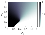
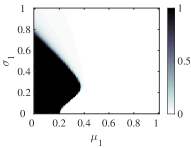
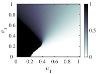
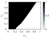
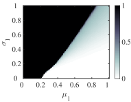
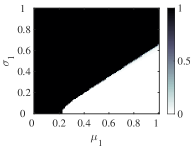
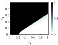
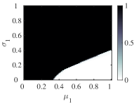
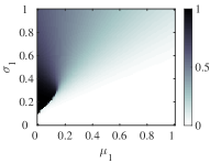
  • (28) In the limit of infinite networks, the clustering coefficient that quantifies the chance that any two neighbors of a given node are also neighbors converges to zero. It means that the network is locally tree-like, i.e., it does not contain short cycles. This then allows us to develop a branching process approximation for the final fraction of failed nodes ρl:=limNρl,Nassignsuperscriptsubscript𝜌𝑙subscript𝑁subscriptsuperscript𝜌𝑙𝑁\rho_{l}^{*}:=\lim_{N\rightarrow\infty}\rho^{*}_{l,N} on each layer l𝑙l in the limit of infinite network size. This approximation is valid for arbitrary degree distributions with finite second moments (Molloy1995; Newman.Strogatz.ea2001Randomgraphswith). For our model, the risk measure is ρ=ρ0superscript𝜌subscriptsuperscript𝜌0\rho^{*}=\rho^{*}_{0}, i.e., the fraction of failed nodes in layer 0 only. However, in order to calculate ρsuperscript𝜌\rho^{*}, we need to calculate both ρlsubscriptsuperscript𝜌𝑙\rho^{*}_{l}, as failures on the two layers are mutually dependent.
  • (29) A node fails initially if it has a negative threshold. Consequently, F0(θ0=0)subscript𝐹0subscript𝜃00F_{0}(\theta_{0}=0) and F1(θ1=0)subscript𝐹1subscript𝜃10F_{1}(\theta_{1}=0) define, for each layer, the initial fraction of failed nodes. These failures can lead to cascades that evolve until the steady states ρlsubscriptsuperscript𝜌𝑙\rho^{*}_{l} on the two layers are reached. We can express the ρlsubscriptsuperscript𝜌𝑙\rho^{*}_{l} as averages with respect to the degree distribution pl(kl)subscript𝑝𝑙subscript𝑘𝑙p_{l}(k_{l}) which we take as input to our model:
    ρl=klpl(kl)(sl=1|kl)subscriptsuperscript𝜌𝑙subscriptsubscript𝑘𝑙subscript𝑝𝑙subscript𝑘𝑙subscript𝑠𝑙conditional1subscript𝑘𝑙\rho^{*}_{l}=\sum_{k_{l}}p_{l}(k_{l})\mathbb{P}(s_{l}=1|k_{l}) (5)
    (sl=1|kl)subscript𝑠𝑙conditional1subscript𝑘𝑙\mathbb{P}(s_{l}=1|k_{l}) is the conditional probability that a node with a given degree klsubscript𝑘𝑙k_{l} on layer l𝑙l fails in layer l𝑙l. In order to calculate this probability, the local tree approximation is essential as it allows us to treat failures of neighbors of a given node as independent events that happen with a failure probability πlsuperscriptsubscript𝜋𝑙\pi_{l}^{*}. Consequently, the number nlsubscript𝑛𝑙n_{l} of failed neighbors of a node of degree klsubscript𝑘𝑙k_{l} in layer l𝑙l follows a binomial distribution so that nlsubscript𝑛𝑙n_{l} neighbors are failed with probability
    B(nl,kl,πl):=(klnl)(1πl)klnl(πl)nl.assign𝐵subscript𝑛𝑙subscript𝑘𝑙subscriptsuperscript𝜋𝑙binomialsubscript𝑘𝑙subscript𝑛𝑙superscript1subscriptsuperscript𝜋𝑙subscript𝑘𝑙subscript𝑛𝑙superscriptsubscriptsuperscript𝜋𝑙subscript𝑛𝑙B(n_{l},k_{l},\pi^{*}_{l}):=\binom{k_{l}}{n_{l}}\left(1-\pi^{*}_{l}\right)^{k_{l}-n_{l}}\left(\pi^{*}_{l}\right)^{n_{l}}. (6)
    This allows us to express (sl=1|kl)subscript𝑠𝑙conditional1subscript𝑘𝑙\mathbb{P}(s_{l}=1|k_{l}) as:
    (sl=1|kl)=nl=0klB(nl,kl,πl)(sl=1|kl,nl,ρs,1l),subscript𝑠𝑙conditional1subscript𝑘𝑙subscriptsuperscriptsubscript𝑘𝑙subscript𝑛𝑙0𝐵subscript𝑛𝑙subscript𝑘𝑙subscriptsuperscript𝜋𝑙subscript𝑠𝑙conditional1subscript𝑘𝑙subscript𝑛𝑙subscriptsuperscript𝜌𝑠1𝑙\mathbb{P}(s_{l}=1|k_{l})=\sum^{k_{l}}_{n_{l}=0}B(n_{l},k_{l},\pi^{*}_{l})\mathbb{P}\left(s_{l}=1|k_{l},n_{l},\rho^{*}_{s,1-l}\right), (7)
    where (sl=1|kl,nl,ρs,1l)subscript𝑠𝑙conditional1subscript𝑘𝑙subscript𝑛𝑙subscriptsuperscript𝜌𝑠1𝑙\mathbb{P}(s_{l}=1|k_{l},n_{l},\rho^{*}_{s,1-l}) is the probability that a node fails in layer l𝑙l given that exactly nlsubscript𝑛𝑙n_{l} of its klsubscript𝑘𝑙k_{l} neighbors failed. This failure results from the fact that the fraction of failed nodes nl/klsubscript𝑛𝑙subscript𝑘𝑙n_{l}/k_{l} exceeded the threshold. This was the original threshold θlsubscript𝜃𝑙\theta_{l} with a probability (1ρs,1l)1subscriptsuperscript𝜌𝑠1𝑙(1-\rho^{*}_{s,1-l}) because the node did not fail in layer (1l)1𝑙(1-l). Or it was the reduced threshold θl(1r(1l)(l))subscript𝜃𝑙1subscript𝑟1𝑙𝑙\theta_{l}(1-r_{(1-l)(l)}) with a probability ρs,1lsubscriptsuperscript𝜌𝑠1𝑙\rho^{*}_{s,1-l} because the node failed in layer (1l)1𝑙(1-l) before. Consequently, we have:
    (sl=1|kl,nl,ρs,1l)=(1ρs,1l)Fl(nlkl)+ρs,1lFl(clnlkl).subscript𝑠𝑙conditional1subscript𝑘𝑙subscript𝑛𝑙subscriptsuperscript𝜌𝑠1𝑙1subscriptsuperscript𝜌𝑠1𝑙subscript𝐹𝑙subscript𝑛𝑙subscript𝑘𝑙subscriptsuperscript𝜌𝑠1𝑙subscript𝐹𝑙subscript𝑐𝑙subscript𝑛𝑙subscript𝑘𝑙\displaystyle\mathbb{P}\left(s_{l}=1|k_{l},n_{l},\rho^{*}_{s,1-l}\right)=\left(1-\rho^{*}_{s,1-l}\right)F_{l}\left(\frac{n_{l}}{k_{l}}\right)+\rho^{*}_{s,1-l}F_{l}\left(c_{l}\frac{n_{l}}{k_{l}}\right). (8)
    Fl(nl/kl)subscript𝐹𝑙subscript𝑛𝑙subscript𝑘𝑙F_{l}\left({n_{l}}/{k_{l}}\right) is the probability that the original threshold is exceeded, whereas Fl(clnl/kl)subscript𝐹𝑙subscript𝑐𝑙subscript𝑛𝑙subscript𝑘𝑙F_{l}\left(c_{l}{n_{l}}/{k_{l}}\right) is the probability that the reduced threshold is exceeded, where c0:=1/(1r10)assignsubscript𝑐011subscript𝑟10c_{0}:=1/(1-r_{10}) and c1:=assignsubscript𝑐1c_{1}:=\infty.
  • (30) Note that ρs,1lsubscriptsuperscript𝜌𝑠1𝑙\rho^{*}_{s,1-l} differs from ρ1lsuperscriptsubscript𝜌1𝑙\rho_{1-l}^{*} used in Eqn. (5). It gives us only the conditional probability that the node has failed in layer (1l)1𝑙(1-l), given that it has not failed in layer l𝑙l. It depends on a neighbor’s failure probability on the other layer, π1lsubscriptsuperscript𝜋1𝑙\pi^{*}_{1-l}, via
    ρs,1l=k1lp1l(k1l)nl=0k1lB(nl,k1l,π1l)F1l(n1lk1l).subscriptsuperscript𝜌𝑠1𝑙subscriptsubscript𝑘1𝑙subscript𝑝1𝑙subscript𝑘1𝑙subscriptsuperscriptsubscript𝑘1𝑙subscript𝑛𝑙0𝐵subscript𝑛𝑙subscript𝑘1𝑙subscriptsuperscript𝜋1𝑙subscript𝐹1𝑙subscript𝑛1𝑙subscript𝑘1𝑙\displaystyle\rho^{*}_{s,1-l}=\sum_{k_{1-l}}p_{1-l}(k_{1-l})\sum^{k_{1-l}}_{n_{l}=0}B(n_{l},k_{1-l},\pi^{*}_{1-l})\ F_{1-l}\left(\frac{n_{1-l}}{k_{1-l}}\right). (9)
    Eqn. (9) has the same structure as the branching process approximation for the fraction of failed nodes on single layers (Gleeson2007). It also has a structure similar to Eqs. (5)-(7), with the only difference of a simpler response function, i.e., (sl=1|kl,nl,ρs,1l)=F1l(n1l/k1l)subscript𝑠𝑙conditional1subscript𝑘𝑙subscript𝑛𝑙subscriptsuperscript𝜌𝑠1𝑙subscript𝐹1𝑙subscript𝑛1𝑙subscript𝑘1𝑙\mathbb{P}(s_{l}=1|k_{l},n_{l},\rho^{*}_{s,1-l})=F_{1-l}(n_{1-l}/k_{1-l}), which is the probability that the fraction of failed neighbors exceeds the original threshold in layer (1l)1𝑙(1-l).
  • (31) In order to compute Eqn. (7), we need to know the failure probability πlsuperscriptsubscript𝜋𝑙\pi_{l}^{*} of a neighbor in layer l𝑙l. To achieve this, we iteratively solve a system of coupled fixed-point equations for the probabilities πlsuperscriptsubscript𝜋𝑙\pi_{l}^{*}, defined as
    πl=Ll(πl):=1zlklpl(kl)klnl=0kl1B(nl,kl1,πl)(sl=1|kl,nl,ρs,1l)subscriptsuperscript𝜋𝑙subscript𝐿𝑙subscriptsuperscript𝜋𝑙assign1subscript𝑧𝑙subscriptsubscript𝑘𝑙subscript𝑝𝑙subscript𝑘𝑙subscript𝑘𝑙subscriptsuperscriptsubscript𝑘𝑙1subscript𝑛𝑙0𝐵subscript𝑛𝑙subscript𝑘𝑙1subscriptsuperscript𝜋𝑙subscript𝑠𝑙conditional1subscript𝑘𝑙subscript𝑛𝑙subscriptsuperscript𝜌𝑠1𝑙\displaystyle\pi^{*}_{l}=L_{l}\left(\pi^{*}_{l}\right):=\frac{1}{z_{l}}\sum_{k_{l}}{p_{l}(k_{l})k_{l}}\sum^{k_{l}-1}_{n_{l}=0}B(n_{l},k_{l}-1,\pi^{*}_{l})\mathbb{P}\left(s_{l}=1|k_{l},n_{l},\rho^{*}_{s,1-l}\right) (10)
    where zl=klpl(kl)klsubscript𝑧𝑙subscriptsubscript𝑘𝑙subscript𝑝𝑙subscript𝑘𝑙subscript𝑘𝑙z_{l}=\sum_{k_{l}}p_{l}(k_{l})k_{l} and (sl=1|kl,nl,ρs,1l)subscript𝑠𝑙conditional1subscript𝑘𝑙subscript𝑛𝑙subscriptsuperscript𝜌𝑠1𝑙\mathbb{P}(s_{l}=1|k_{l},n_{l},\rho^{*}_{s,1-l}) is defined by Eqn. (8)
  • (32) We note again similarities between Eqn. (10) that describes the failure probability of a neighbor and Eqs. (5), (8) that describe the failure probability of a node, but also two differences:
  • (33) a) In Eqn. (10) the degree distribution of a neighbor follows pl(kl)kl/zlsubscript𝑝𝑙subscript𝑘𝑙subscript𝑘𝑙subscript𝑧𝑙{p_{l}(k_{l})k_{l}}/{z_{l}} instead of pl(kl)subscript𝑝𝑙subscript𝑘𝑙p_{l}(k_{l}) for a node (Newman2010). It is proportional to the degree klsubscript𝑘𝑙k_{l}, since every link of a neighbor increases the probability of the neighbor to be connected to the node under consideration.
  • (34) b) The binomial distribution in Eqn. (10) depends on kl1subscript𝑘𝑙1k_{l}-1 instead of klsubscript𝑘𝑙k_{l} because we have to take into account the second-order neighborhood of the node under consideration. We take the failure probability of a neighbor as input to calculate the failure probability of the node under consideration as in Eqs. (5), (8). Therefore, πlsubscriptsuperscript𝜋𝑙\pi^{*}_{l} is conditioned on the event that the node under consideration has not failed before the neighbor. Only kl1subscript𝑘𝑙1k_{l}-1 neighbors of the neighbor with degree klsubscript𝑘𝑙k_{l} can have possibly failed before, because the node under consideration is a neighbor of this neighbor.
  • (35)
  • (36)
  • 4 Results

  • (37)
  • (38)
  • 4.1 Comparison with computer simulations

  • (39) We now compare our numerical solution of the fixed point equations (10) with computer simulations, using the illustrative case of an uncorrelated, two-layer Erdős-Rényi network (ErdosRenyi). For the computer simulations, we implement the time-dependent model as described in Sect. 2, i.e. we simulate the evolution of cascades until they reach the steady state. The network size is N=10,000𝑁10000N=10,000 for each layer. Further, we sample over 100100100 network realizations for every initial condition. The degree distributions pl(kl)subscript𝑝𝑙subscript𝑘𝑙p_{l}(k_{l}) on each layer are approximately Poisson distributions
    pl(kl)=zlklkl!ezlsubscript𝑝𝑙subscript𝑘𝑙superscriptsubscript𝑧𝑙subscript𝑘𝑙subscript𝑘𝑙superscript𝑒subscript𝑧𝑙p_{l}(k_{l})=\frac{z_{l}^{k_{l}}}{k_{l}!}\ e^{-z_{l}} (11)
    with identical mean degrees z0=z1subscript𝑧0subscript𝑧1z_{0}=z_{1}. The thresholds are normally distributed, i.e. θ0𝒩(μ0,σ02)similar-tosubscript𝜃0𝒩subscript𝜇0subscriptsuperscript𝜎20\theta_{0}\sim\mathcal{N}(\mu_{0},\sigma^{2}_{0}) and θ1𝒩(μ1,σ12)similar-tosubscript𝜃1𝒩subscript𝜇1subscriptsuperscript𝜎21\theta_{1}\sim\mathcal{N}(\mu_{1},\sigma^{2}_{1}) with different parameters μlsubscript𝜇𝑙\mu_{l}, σlsubscript𝜎𝑙\sigma_{l}. In our case, we fix the threshold distribution on layer 0 to parameters μ0=0.3subscript𝜇00.3\mu_{0}=0.3 and σ0=0.1subscript𝜎00.1\sigma_{0}=0.1, which ensures that the failure probability for the nodes in an uncoupled network would be very small, i.e., 0.00450.00450.0045. We vary the parameters μ1subscript𝜇1\mu_{1} and σ1subscript𝜎1\sigma_{1} of layer 1, to study the emergence of large cascades on layer 0 because of the coupling with strength r10subscript𝑟10r_{10}.
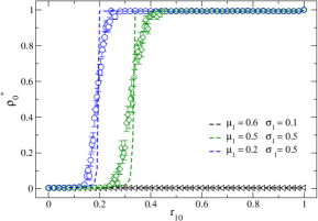
  • (40) Figure 2 demonstrates that a small variation in the coupling strength r10subscript𝑟10r_{10} may result in a rapid shift from a regime with almost no failures (ρ00subscriptsuperscript𝜌00\rho^{*}_{0}\approx 0) to a regime of complete system failure (ρ01subscriptsuperscript𝜌01\rho^{*}_{0}\approx 1). The coupling strength at the onset of this regime shift, r10csuperscriptsubscript𝑟10𝑐r_{10}^{c}, depends on the parameters of the threshold distribution on layer 1 (i.e. μ1subscript𝜇1\mu_{1} and σ1subscript𝜎1\sigma_{1}). Namely, r10csuperscriptsubscript𝑟10𝑐r_{10}^{c} is increasing in μ1subscript𝜇1\mu_{1}. For certain parameter constellations (e.g. μ1=0.6subscript𝜇10.6\mu_{1}=0.6 and σ2=0.1subscript𝜎20.1\sigma_{2}=0.1), we also find no failure cascades at all, which will be further discussed in Fig. 4. Finally, we note the excellent match between the numerical and the simulation results. The differences in the slope result from the fact that we have simulated finite networks, whereas the fixed point equations holds for infinite networks.
  • (41)
  • Refer to caption

    Figure 2: Sharp Regime Change in Threshold-Feedback Model: ρ0subscriptsuperscript𝜌0\rho^{*}_{0} for different combinations of threshold distributions, as the coupling strength r10subscript𝑟10r_{10} is varied. The threshold distribution on the core-business layer is set to 𝒩(0.3,0.12)𝒩0.3superscript0.12\mathcal{N}(0.3,0.1^{2}) while the threshold distribution on the subsidiary-business layer is 𝒩(0.6,0.12)𝒩0.6superscript0.12\mathcal{N}(0.6,0.1^{2}) (black curve), 𝒩(0.5,0.52)𝒩0.5superscript0.52\mathcal{N}(0.5,0.5^{2}) (green curve) and 𝒩(0.2,0.52)𝒩0.2superscript0.52\mathcal{N}(0.2,0.5^{2}) (blue curve). The two layers are independent Erdős-Rényi networks with mean degrees z0=z1=5subscript𝑧0subscript𝑧15z_{0}=z_{1}=5. The dotted lines are the curves predicted by our analytics, while with the open symbols we show simulation results on Erdős-Rényi networks with 10000 nodes where each point is averaged over 100 realizations. The error bars indicate the size of the standard error.
  • (42)
  • (43)
  • 4.2 Impact of the coupling strength

  • (44) To gain a broader understanding of how the coupling between the two layers can cause such a rapid transition from a low-risk regime (i.e. ρ00subscriptsuperscript𝜌00\rho^{*}_{0}\approx 0) to a catastrophic one (i.e. ρ01subscriptsuperscript𝜌01\rho^{*}_{0}\approx 1), we calculate the (μ1,σ1)subscript𝜇1subscript𝜎1(\mu_{1},\sigma_{1}) phase diagram for various coupling strengths. The results are shown in Fig. 3, where dark areas indicate parameter constellations with a very high fraction of failed nodes. The left column shows the measure of systemic risk ρ0superscriptsubscript𝜌0\rho_{0}^{*}, which is equivalent to the fraction of failed nodes in layer 0, whereas the middle column shows the corresponding fraction of failed nodes in layer 1.
  • (45)
  • ρ0subscriptsuperscript𝜌0\rho^{*}_{0} ρ1subscriptsuperscript𝜌1\rho^{*}_{1} ρaggsubscriptsuperscript𝜌agg\rho^{*}_{\text{agg}}
    r10=0subscript𝑟100r_{10}=0 Refer to caption Refer to caption Refer to caption
  • (46) r10=0.2subscript𝑟100.2r_{10}=0.2
  • Refer to caption Refer to caption Refer to caption
    r10=0.4subscript𝑟100.4r_{10}=0.4 Refer to caption Refer to caption Refer to caption
    r10=0.8subscript𝑟100.8r_{10}=0.8 Refer to caption Refer to caption Refer to caption
    r10=1.0subscript𝑟101.0r_{10}=1.0 Refer to caption Refer to caption Refer to caption
    Figure 3: Sharp Regime Change in Threshold-Feedback Model: ρ0subscriptsuperscript𝜌0\rho^{*}_{0} and ρ1subscriptsuperscript𝜌1\rho^{*}_{1} for μ0=0.3subscript𝜇00.3\mu_{0}=0.3, σ0=0.1subscript𝜎00.1\sigma_{0}=0.1 and (μ1,σ1)[0,1]2subscript𝜇1subscript𝜎1superscript012(\mu_{1},\sigma_{1})\in[0,1]^{2} as r10subscript𝑟10r_{10} is varied. The two layers are independent Erdős-Rényi networks with mean degrees z0=z1=5subscript𝑧0subscript𝑧15z_{0}=z_{1}=5 and thresholds on each layer are independently distributed, i.e. θ0𝒩(0.3,0.12)similar-tosubscript𝜃0𝒩0.3superscript0.12\theta_{0}\sim\mathcal{N}(0.3,0.1^{2}) and θ1𝒩(μ1,σ12)similar-tosubscript𝜃1𝒩subscript𝜇1subscriptsuperscript𝜎21\theta_{1}\sim\mathcal{N}(\mu_{1},\sigma^{2}_{1}), where (μ1,σ1)[0,1]2subscript𝜇1subscript𝜎1superscript012(\mu_{1},\sigma_{1})\in[0,1]^{2}. ρaggsubscriptsuperscript𝜌𝑎𝑔𝑔\rho^{*}_{agg} is the fraction of failures on the aggregated network, i.e. a network where kagg=k0+k1subscript𝑘𝑎𝑔𝑔subscript𝑘0subscript𝑘1k_{agg}=k_{0}+k_{1} and θagg=θ0+θ1subscript𝜃𝑎𝑔𝑔subscript𝜃0subscript𝜃1\theta_{agg}=\theta_{0}+\theta_{1}.
  • (47) As a reference case, the right column shows a single-layer network, which we constructed in order to put the results for the two-layer network into perspective. Nodes in this combined single-layer network have a degree kagg=k0+k1subscript𝑘𝑎𝑔𝑔subscript𝑘0subscript𝑘1k_{agg}=k_{0}+k_{1} and a threshold θagg=θ0+θ1subscript𝜃𝑎𝑔𝑔subscript𝜃0subscript𝜃1\theta_{agg}=\theta_{0}+\theta_{1}, i.e. we simply sum up the two values per node that were distributed on the two layers before. The degree distribution can be found using the convolution of p0(k0)subscript𝑝0subscript𝑘0p_{0}(k_{0}) and p1(k1)subscript𝑝1subscript𝑘1p_{1}(k_{1}), i.e. pagg(kagg)=(p0p1)(kagg)subscript𝑝𝑎𝑔𝑔subscript𝑘𝑎𝑔𝑔subscript𝑝0subscript𝑝1subscript𝑘𝑎𝑔𝑔p_{agg}(k_{agg})=(p_{0}\ast p_{1})(k_{agg}). The latter can be shown to be a Poisson distribution with mean degree zagg=z0+z1subscript𝑧𝑎𝑔𝑔subscript𝑧0subscript𝑧1z_{agg}=z_{0}+z_{1}, which is the degree distribution of an infinite Erdős-Rényi network. The threshold distribution for the combined layers can be found by taking the convolution of the probability density functions of θ0subscript𝜃0\theta_{0} and θ1subscript𝜃1\theta_{1}. This yields θagg𝒩(μagg,σagg2)similar-tosubscript𝜃𝑎𝑔𝑔𝒩subscript𝜇𝑎𝑔𝑔subscriptsuperscript𝜎2𝑎𝑔𝑔\theta_{agg}\sim\mathcal{N}(\mu_{agg},\sigma^{2}_{agg}), where μagg=μ0+μ1subscript𝜇𝑎𝑔𝑔subscript𝜇0subscript𝜇1\mu_{agg}=\mu_{0}+\mu_{1} and σagg=σ02+σ12subscript𝜎𝑎𝑔𝑔superscriptsubscript𝜎02superscriptsubscript𝜎12\sigma_{agg}=\sqrt{\sigma_{0}^{2}+\sigma_{1}^{2}}.
  • (48) Our reference case is motivated by two considerations: (a) We want to estimate the error made if a multiplex network is approximated by a single layer network, i.e. the properties of the different layers are simply aggregated in one layer. (b) For the application scenario at hand, namely the management decision of firms to merge their core and subsidiary business units into one business, we want to understand the impact on the resulting risk exposure. To calculate the phase diagram, we assume that all firms make the same decision, which for example could be motivated by herding behavior.
  • (49) Since we vary only (μ1,σ1)subscript𝜇1subscript𝜎1(\mu_{1},\sigma_{1}), we plot all phase diagrams with respect to these two parameters. Because the combined layer network no longer contains the coupling strength r10subscript𝑟10r_{10}, the respective phase plots do not change by varying r10subscript𝑟10r_{10}. They are merely repeated for the purpose of comparison with the other columns. We hypothesize that nodes in the combined layer network have a smaller failure probability compared to the two-layer network because their threshold is much higher. Their degree is also larger, which implies that the risk is better diversified among the neighbors. On the other hand, because of the larger degrees, there is a higher connectivity in the combined layer network. This has the potential to amplify small cascades more than in the less connected separate layers. We will investigate, by means of numerical solutions of the fixed point equations, which of these antagonistic effects may dominate in a given parameter region.
  • (50) By comparing the first and third columns in Fig. 3, we see a different risk profile for small and for large coupling strengths. For small values of r10subscript𝑟10r_{10} the cascades on layer 1 cannot propagate to layer 0, therefore we do not observe any systemic risk. This is different for the combined layer network, where large cascades can occur for a small range of parameters.
  • (51) The picture is inverted for larger values of r10subscript𝑟10r_{10}. Here we find, by increasing r10subscript𝑟10r_{10}, an increasing region of high systemic risk that is driven by the mutual amplification of cascades between the two layers. This leads to a very sharp phase transition, i.e. a clear separation of regions with complete breakdown and regions with no breakdown. We note that this differs from the observation for the combined layer network, where the phase transition can also be observed. However, there are extended regions where the systemic risk is at intermediate levels, as indicated by the gray areas.
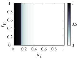
  • (52) We also wish to see how the onset of systemic risk on layer 0 depends on the coupling strength r10subscript𝑟10r_{10}. Thus, in addition to fixing μ0subscript𝜇0\mu_{0} and σ0subscript𝜎0\sigma_{0}, we set σ1subscript𝜎1\sigma_{1} to a small value and plot the phase diagram with respect to (μ1,r10)subscript𝜇1subscript𝑟10(\mu_{1},r_{10}). Fig. 4, for the same columns as in Fig. 3, shows that there is indeed a critical value r10csuperscriptsubscript𝑟10𝑐r_{10}^{c} which is independent of μ1subscript𝜇1\mu_{1}. Below r10csuperscriptsubscript𝑟10𝑐r_{10}^{c}, we do not observe any systemic risk in layer 0, whereas in the combined layer network, we find a considerable systemic risk for small values of μ1subscript𝜇1\mu_{1}. Above r10csuperscriptsubscript𝑟10𝑐r_{10}^{c}, we see in the two-layer network a sharp phase transition between full and no systemic risk that depends on a critical value μ1csuperscriptsubscript𝜇1𝑐\mu_{1}^{c}. Consequently, we study the transition line r10(μ1)subscript𝑟10subscript𝜇1r_{10}(\mu_{1}) in the following subsection.
  • (53)
  • ρ0subscriptsuperscript𝜌0\rho^{*}_{0} ρ1subscriptsuperscript𝜌1\rho^{*}_{1} ρaggsubscriptsuperscript𝜌agg\rho^{*}_{\text{agg}}
  • (54) Refer to caption
  • Refer to caption Refer to caption
    Figure 4: Sharp Regime Change in Threshold-Feedback Model: ρ0subscriptsuperscript𝜌0\rho^{*}_{0} and ρ1subscriptsuperscript𝜌1\rho^{*}_{1} for μ0=0.3subscript𝜇00.3\mu_{0}=0.3, σ0=0.1subscript𝜎00.1\sigma_{0}=0.1 and σ1=0.3subscript𝜎10.3\sigma_{1}=0.3 as μ1subscript𝜇1\mu_{1} and r10subscript𝑟10r_{10} are varied. The two layers are independent Erdős-Rényi networks with mean degrees z0=z1=5subscript𝑧0subscript𝑧15z_{0}=z_{1}=5 and the thresholds on each layer are independently distributed, i.e. θ0𝒩(0.3,0.12)similar-tosubscript𝜃0𝒩0.3superscript0.12\theta_{0}\sim\mathcal{N}(0.3,0.1^{2}) and θ1𝒩(μ1,0.32)similar-tosubscript𝜃1𝒩subscript𝜇1superscript0.32\theta_{1}\sim\mathcal{N}(\mu_{1},0.3^{2}), where μ1[0,1]subscript𝜇101\mu_{1}\in[0,1]. ρaggsubscriptsuperscript𝜌𝑎𝑔𝑔\rho^{*}_{agg} is the fraction of failures on the aggregated network, i.e. a network where kagg=k0+k1subscript𝑘𝑎𝑔𝑔subscript𝑘0subscript𝑘1k_{agg}=k_{0}+k_{1} and θagg=θ0+θ1subscript𝜃𝑎𝑔𝑔subscript𝜃0subscript𝜃1\theta_{agg}=\theta_{0}+\theta_{1}.
  • (55)
  • (56)
  • 4.3 Scaling behavior

  • (57) In Fig. 3 we observe that the sharp phase transition scales almost linearly for large enough coupling strength r10subscript𝑟10r_{10}, i.e.
    σ1=s1μ1+s0forμ10.4,r10r10cformulae-sequencesubscript𝜎1subscript𝑠1subscript𝜇1subscript𝑠0formulae-sequenceforsubscript𝜇10.4subscript𝑟10superscriptsubscript𝑟10𝑐\sigma_{1}=s_{1}\mu_{1}+s_{0}\quad\mathrm{for}\;\mu_{1}\geq 0.4,\;r_{10}\geq r_{10}^{c} (12)
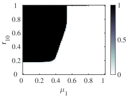
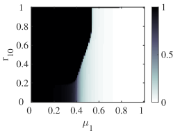
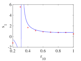
    In order to determine the scaling parameter s1subscript𝑠1s_{1}, we take the phase transition line from the phase diagrams of Fig. 3, which were also calculated for r10=subscript𝑟10absentr_{10}=0.3, 0.5, 0.6, 0.7, 0.9. These lines are approximated by a linear regression, and the slopes obtained this way are plotted in Fig. 5 (left, red dots) against the coupling strength r10subscript𝑟10r_{10}. We observe a non-monotonous dependence of the slope, with a saturation effect for large r10subscript𝑟10r_{10}. Thus, we want to determine r10csuperscriptsubscript𝑟10𝑐r_{10}^{c} and s1(r10)subscript𝑠1subscript𝑟10s_{1}(r_{10}) for r10r10csubscript𝑟10superscriptsubscript𝑟10𝑐r_{10}\geq r_{10}^{c} .
  • (58)
  • Single layer ρsinglesubscriptsuperscript𝜌single\rho^{*}_{\text{single}} Slope s1subscript𝑠1s_{1} ρ0subscriptsuperscript𝜌0\rho^{*}_{0} for r10=0.3subscript𝑟100.3r_{10}=0.3
  • (59) Refer to caption
  • Refer to caption Refer to caption
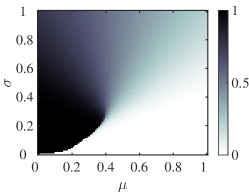
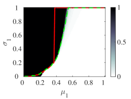
    Figure 5: (Left): Red Circles: Slope s1subscript𝑠1s_{1} of the linear phase transition obtained by linear regression of ρ0subscriptsuperscript𝜌0\rho^{*}_{0} that we calculated by solving the fixed point equations (10) numerically for different values of r10subscript𝑟10r_{10}. The blue curve shows the approximate values for the slopes provided by Eqn. 19. (Middle): Phase diagram for the final cascade size on a single layer without threshold feedback for Poisson random graphs with average degree z=5𝑧5z=5 and normally distributed thresholds Fθ𝒩(μ,σ2)similar-tosubscript𝐹𝜃𝒩𝜇superscript𝜎2F_{\theta}\sim\mathcal{N}\left(\mu,\sigma^{2}\right). (Right): Final cascade size on layer 0, i.e. ρ0subscriptsuperscript𝜌0\rho^{*}_{0}, for r10=0.3subscript𝑟100.3r_{10}=0.3. The red line marks the phase transition defined by the criterion ρsingleρs,1csubscriptsuperscript𝜌singlesubscriptsuperscript𝜌𝑐𝑠1\rho^{*}_{\text{single}}\geq\rho^{c}_{s,1}. The green line corresponds to ρsingle0.45subscriptsuperscript𝜌single0.45\rho^{*}_{\text{single}}\geq 0.45.
  • (60) To better understand this dependence, we perform a linear approximation of L0subscript𝐿0L_{0} in Eqn. (10) as
    L0(π0)a+bπ0subscript𝐿0subscript𝜋0𝑎𝑏subscript𝜋0L_{0}\left(\pi_{0}\right)\approx a+b\pi_{0} (13)
    which is valid for small values of the failure probability π0subscript𝜋0\pi_{0}. Instead of solving the full system of fixed point equations Eqn. (10), we only solve the linearized system in order to deduce criteria for the growth behavior of π0subscript𝜋0\pi_{0} in the fixed point iterations. The fixed point of the linear equation (13) exceeds one if
    a1b1𝑎1𝑏1\displaystyle\frac{a}{1-b}\geq 1 (14)
    Under this condition, initial failures in both layers result in large cascades in layer 0.
  • (61) Eqn. (14) leads to conditions for the parameters μ1csuperscriptsubscript𝜇1𝑐\mu_{1}^{c}, σ1csuperscriptsubscript𝜎1𝑐\sigma_{1}^{c} and r10csuperscriptsubscript𝑟10𝑐r_{10}^{c} if we know the expressions for a𝑎a and b𝑏b. These are obtained from the linearization of Eqn. (10):
    a=𝑎absent\displaystyle a= (s0=1|k0,n0=0,ρs,1),\displaystyle\mathbb{P}\left(s_{0}=1|k_{0},n_{0}=0,\rho^{*}_{s,1}\right),
    b=𝑏absent\displaystyle b= k0=1k0(k01)z0p0(k0)×\displaystyle\sum^{\infty}_{k_{0}=1}\frac{k_{0}(k_{0}-1)}{z_{0}}p_{0}\left(k_{0}\right)\times (15)
    ×[(s0=1|k0,n0=1,ρs,1)(s0=1|k0,n0=0,ρs,1)].\displaystyle\times\left[\mathbb{P}\left(s_{0}=1|k_{0},n_{0}=1,\rho^{*}_{s,1}\right)-\mathbb{P}\left(s_{0}=1|k_{0},n_{0}=0,\rho^{*}_{s,1}\right)\right].
    These parameters depend on the failure probability ρs,1superscriptsubscript𝜌𝑠1\rho_{s,1}^{*} of a node in the other layer, i.e. layer 1.
  • (62) For the further discussion, we first concentrate on the worst case scenario ρs,1=1superscriptsubscript𝜌𝑠11\rho_{s,1}^{*}=1, i.e. all nodes failed on layer 1. We are interested in identifying the regime where even in the worst case, cascades in layer 1 do not propagate to layer 0. In other words, we want to approximate the critical coupling r10csubscriptsuperscript𝑟𝑐10r^{c}_{10} above which we can observe regions of high systemic risk in the left column of Fig. 4. With ρs,1=1superscriptsubscript𝜌𝑠11\rho_{s,1}^{*}=1 the parameters a𝑎a and b𝑏b simplify to
    a=F0(0),b=k0=1k0(k01)z0p0(k0)[F0(1k0(1r10))F0(0)].formulae-sequence𝑎subscript𝐹00𝑏subscriptsuperscriptsubscript𝑘01subscript𝑘0subscript𝑘01subscript𝑧0subscript𝑝0subscript𝑘0delimited-[]subscript𝐹01subscript𝑘01subscript𝑟10subscript𝐹00\displaystyle\begin{split}&a=F_{0}(0),\\ &b=\sum^{\infty}_{k_{0}=1}\frac{k_{0}(k_{0}-1)}{z_{0}}p_{0}\left(k_{0}\right)\left[F_{0}\left(\frac{1}{k_{0}\left(1-r_{10}\right)}\right)-F_{0}(0)\right].\end{split} (16)
    We note that these are independent of μ1subscript𝜇1\mu_{1}, σ1subscript𝜎1\sigma_{1}. For the set of parameters used in Fig. 4, we obtain with the help of Eqn. ((61)) and Eqn. (14) the value of the critical coupling r10c=0.204subscriptsuperscript𝑟𝑐100.204r^{c}_{10}=0.204. In comparison with the numerical calculation r10=0.18subscript𝑟100.18r_{10}=0.18, which takes the full set of fixed point equations into account, this is a good approximation. That means large cascades can propagate from layer 1 to layer 0 above a critical coupling strength r10c0.2similar-to-or-equalssubscriptsuperscript𝑟𝑐100.2r^{c}_{10}\simeq 0.2. This holds independently of μ1subscript𝜇1\mu_{1} and σ1subscript𝜎1\sigma_{1}.
  • (63) Next we explain the dependence s1(r10)subscript𝑠1subscript𝑟10s_{1}(r_{10}) as shown in Fig. 3. By this we estimate the slope of the phase transition line (which is of the form σ1s1μ1proportional-tosubscript𝜎1subscript𝑠1subscript𝜇1\sigma_{1}\propto s_{1}\mu_{1}). Again, we deduce this relation from Eqs. (14), ((61)), but this time we cannot use ρs,1=1subscriptsuperscript𝜌𝑠11\rho^{*}_{s,1}=1. For ρs,11subscriptsuperscript𝜌𝑠11\rho^{*}_{s,1}\neq 1, we automatically obtain a dependence on the threshold parameters μ1subscript𝜇1\mu_{1} and σ1subscript𝜎1\sigma_{1} of layer 1. Combining Eqn. ((61)) and Eqn. (14), we can define a critical value ρs,1csubscriptsuperscript𝜌𝑐𝑠1\rho^{c}_{s,1} such that Eqn. (14) is satisfied for ρs,1ρs,1csubscriptsuperscript𝜌𝑠1subscriptsuperscript𝜌𝑐𝑠1\rho^{*}_{s,1}\geq\rho^{c}_{s,1}:
    ρs,1c:=1+F0(0)(z01)c0(0)c0(r)c0(0),assignsubscriptsuperscript𝜌𝑐𝑠11subscript𝐹00subscript𝑧01subscript𝑐00subscript𝑐0𝑟subscript𝑐00\displaystyle\rho^{c}_{s,1}:=\frac{1+F_{0}(0)(z_{0}-1)-c_{0}(0)}{c_{0}(r)-c_{0}(0)}, (17)
    where
    c0(r):=k0=1k0(k01)z0p0(k0)F0(1k0(1r10)).assignsubscript𝑐0𝑟subscriptsuperscriptsubscript𝑘01subscript𝑘0subscript𝑘01subscript𝑧0subscript𝑝0subscript𝑘0subscript𝐹01subscript𝑘01subscript𝑟10\displaystyle c_{0}(r):=\sum^{\infty}_{k_{0}=1}\frac{k_{0}(k_{0}-1)}{z_{0}}p_{0}\left(k_{0}\right)F_{0}\left(\frac{1}{k_{0}\left(1-r_{10}\right)}\right). (18)
    This is a reformulation of Eqn. (14), which gives us an estimation of when to expect large cascades in layer 0. Still, we do not know ρs,1subscriptsuperscript𝜌𝑠1\rho^{*}_{s,1} without solving the full system of fixed point equations (10). In the following we test two proxies for ρs,1subscriptsuperscript𝜌𝑠1\rho^{*}_{s,1} which lead us to a linear dependence between μ1subscript𝜇1\mu_{1} and σ1subscript𝜎1\sigma_{1}.
  • (64) (1) The initial value ρs,1(t=0)=F1(0)=Φ(μ1/σ1)subscript𝜌𝑠1𝑡0subscript𝐹10Φsubscript𝜇1subscript𝜎1\rho_{s,1}(t=0)=F_{1}(0)=\Phi\left(-{\mu_{1}}/{\sigma_{1}}\right) is already enough to determine the growth of π0subscript𝜋0\pi_{0} in the early stages of the fixed point iterations. Especially for larger values of r10subscript𝑟10r_{10}, a large cascade in layer 0 might be already triggered just by the initial failures in layer 1. Therefore, we set ρs,1cF1(0)similar-to-or-equalssubscriptsuperscript𝜌𝑐𝑠1subscript𝐹10\rho^{c}_{s,1}\simeq F_{1}(0), which results in
    σ1μ1/Φ1(ρs,1c),proportional-tosubscript𝜎1subscript𝜇1superscriptΦ1subscriptsuperscript𝜌𝑐𝑠1\displaystyle\sigma_{1}\propto-\mu_{1}/\Phi^{-1}\left(\rho^{c}_{s,1}\right), (19)
    i.e.,
    s1=1/Φ1(ρs,1c)subscript𝑠11superscriptΦ1subscriptsuperscript𝜌𝑐𝑠1s_{1}=-{1}/{\Phi^{-1}\left(\rho^{c}_{s,1}\right)} (20)
    where Φ1superscriptΦ1\Phi^{-1} denotes the cumulative distribution function of the standard normal distribution. We plot this slope using a blue line in Fig. 5(left), to demonstrate the good agreement of our approximation with the numerical slopes s1subscript𝑠1s_{1} for r100.4subscript𝑟100.4r_{10}\geq 0.4.
  • (65) (2) For smaller coupling strengths r10subscript𝑟10r_{10} we test a second proxy for ρs,1subscriptsuperscript𝜌𝑠1\rho^{*}_{s,1}. A lower bound for ρs,1subscriptsuperscript𝜌𝑠1\rho^{*}_{s,1} is given by the final cascade size on a single layer ρsinglesubscriptsuperscript𝜌single\rho^{*}_{\text{single}}, where no feedback mechanism with another layer exists. That means, the other layer cannot further amplify the failures. Cascades in single layers have been studied in Burkholz2015. We use their approach to plot a phase diagram for the final cascade size for Poisson random graphs with average degree z=5𝑧5z=5, shown in the middle panel of Fig. 5.
  • (66) When we compare the plots of Fig. 3 (left) with Fig. 5 (middle), we observe that in the parameter regions in Fig. 3 (left) where no cascades occur, also no cascades occur in Fig. 5 (middle). This holds only for strong couplings r10subscript𝑟10r_{10}. Consequently, in this limit, our second proxy for ρs,1subscriptsuperscript𝜌𝑠1\rho^{*}_{s,1} gives similar results as our first proxy.
  • (67) However, the second proxy for ρs,1subscriptsuperscript𝜌𝑠1\rho^{*}_{s,1}, is the more general one as we can also correctly cover the transition line for values of 0.2μ10.40.2subscript𝜇10.40.2\leq\mu_{1}\leq 0.4. In this range, the transition line is largely independent of the value r10subscript𝑟10r_{10}. It basically coincides with the transition line for ρsinglesubscriptsuperscript𝜌single\rho^{*}_{\text{single}}, the fraction of failed nodes for single layer networks.
  • (68) For values of μ1subscript𝜇1\mu_{1} larger than 0.4 and for weak coupling, e.g. for r10=0.3subscript𝑟100.3r_{10}=0.3, we observe in Fig. 5 (right, red line) that the transition line is no longer accurately described. The condition ρsingleρs,1c=0.55subscriptsuperscript𝜌singlesubscriptsuperscript𝜌𝑐𝑠10.55\rho^{*}_{\text{single}}\geq\rho^{c}_{s,1}=0.55 gives only an upper bound for the transition line, but not a lower one. We observe that already cascade sizes of ρsingle0.45subscriptsuperscript𝜌single0.45\rho^{*}_{\text{single}}\geq 0.45 lead to large cascade amplification on layer 0, due to nonlinear effects. I.e. the green dotted line in Fig. 5 (right) gives an almost perfect match with the numerically calculated transition line.
  • (69) That means, we can even generalize our statement that the transition line for ρsinglesubscriptsuperscript𝜌single\rho^{*}_{\text{single}} determines the phase transition. This holds not only for small μ1subscript𝜇1\mu_{1}, but also for larger μ1subscript𝜇1\mu_{1} and a broad range of the coupling strength r10subscript𝑟10r_{10}.
  • (70)
  • (71)
  • 5 Conclusions

  • (72) Our paper essentially addresses the problem of whether systemic risk is increased or decreased if, instead of a single-layer network, a two-layer representation is used. In the latter, the nodes of the network appear on two layers 0 and 1 with different properties. Specifically, they have different degree distributions p0(k0)subscript𝑝0subscript𝑘0p_{0}\left(k_{0}\right), p1(k1)subscript𝑝1subscript𝑘1p_{1}\left(k_{1}\right) and different threshold distributions F0(θ0)subscript𝐹0subscript𝜃0F_{0}\left(\theta_{0}\right), F1(θ1)subscript𝐹1subscript𝜃1F_{1}\left(\theta_{1}\right). There is an asymmetric coupling between the two layers such that nodes that failed on layer 0 also fail on layer 1. However, nodes that did not fail on layer 0, may still fail on layer 1 because of a cascade dynamics on layer 1. In this case, their failing threshold on layer 0 is reduced by a fraction r10subscript𝑟10r_{10}, where r10subscript𝑟10r_{10} denotes the coupling strength between the two layers.
  • (73) The mutual feedback between the two layers can then result in the amplification of failure cascades, which we study analytically. We can calculate a variable ρlsuperscriptsubscript𝜌𝑙\rho_{l}^{*} which is the final fraction of failed nodes on each layer l{0,1}𝑙01l\in\{0,1\}. Our measure of systemic risk is ρρ0superscript𝜌superscriptsubscript𝜌0\rho^{*}\equiv\rho_{0}^{*}, i.e. we only consider whether nodes have failed on layer 0. Obviously, if r10subscript𝑟10r_{10} is small, no failure cascade in layer 1 can propagate to layer 0. In this case, whether or not we observe failure cascades only depends on the conditions in layer 0. These conditions are expressed by the parameters of the threshold distribution, μ0subscript𝜇0\mu_{0} and σ0subscript𝜎0\sigma_{0}, which are chosen so that no failure cascade occurs. By varying r10subscript𝑟10r_{10}, we then study the impact of failures on layer 1 on failures on layer 0. We derive an analytical approach to calculate ρlsubscriptsuperscript𝜌𝑙\rho^{*}_{l}, which leads to a system of coupled fixed point equations solved numerically.
  • (74) Our results are visualized by means of phase diagrams that show, for various parameter constellations, the value of the main risk measure ρ=ρ0superscript𝜌subscriptsuperscript𝜌0\rho^{*}=\rho^{*}_{0}. The most prominent feature is the existence of a very sharp phase transition between a regime of no systemic risk and a regime of full collapse. This means that small changes in the parameters μ1subscript𝜇1\mu_{1} and σ1subscript𝜎1\sigma_{1}, describing the threshold distribution on layer 1, can lead to an abrupt regime shift. Our task was then to approximate this line of transition in terms of the coupling strength r10subscript𝑟10r_{10} and the parameters of the threshold distribution. Subsequently, we use these insights to compare the systemic risk in single-layer and two-layer networks.
  • (75) The derivation of mathematical approximations for the phase transitions that are compared, and confirmed, by numerical solutions of the full problem has a value on its own. Here, we focus on the conclusions that can be made based on these calculations. First of all, we understand that systemic risk is reduced in the two-layer network only if the coupling strength between the two layers is rather small. Above a critical value r10c=0.2superscriptsubscript𝑟10𝑐0.2r_{10}^{c}=0.2, which is also estimated analytically, failures on layer 1 are amplified on layer 0 and thus lead to an increase of the systemic risk. If we compare this with the reference case of a single layer network, we find that the systemic risk is smaller there, for most ranges of the parameters. Hence, above a critical coupling, it is not beneficial to split the network into two layers, if systemic risk shall be mitigated.
  • (76) Our findings can be applied to a scenario where firms have to decide whether to split their business into a less risky core business, essential for their survival, and a subsidiary business, which can be more risky. Such a split leads to the representation of the (same) firm on two different levels 0 and 1, where the latter has a larger risk of failure cascades. This decision only leads to less failure risk for the firm if the coupling between the core business layer and the subsidiary business layer is weak enough. Close to the transition line between the no-risk and the high-risk regime, slight changes in the firms’ failure thresholds or in the coupling between the different businesses may potentially cause the system to collapse completely.
  • (77) There is another important conclusion to be drawn for firms that already have their activities split between a less risky core business and a more risky subsidiary business. If such firms estimate systemic risk based on an aggregated network representation with only one layer instead of the two-layer representation, they may systematically underestimate the real risk, in particular if the coupling is still strong. As we have shown, under such conditions the systemic risk in the aggregated network is lower than in the two-layer network. Hence, there can be drastic consequences from drawing conclusions based on an inappropriate aggregated picture.
  • (78)
  • (79)
  • Acknowledgements.

    R. Burkholz acknowledges support by the ETH48 project, A. Garas and F. Schweitzer acknowledge support by the EU-FET project MULTIPLEX 317532. The authors thank I. Scholtes for discussions.

  • (80)
  • (81)