Doubly Decomposing
Nonparametric Tensor Regression

Abstract

Nonparametric extension of tensor regression is proposed. Nonlinearity in a high-dimensional tensor space is broken into simple local functions by incorporating low-rank tensor decomposition. Compared to naive nonparametric approaches, our formulation considerably improves the convergence rate of estimation while maintaining consistency with the same function class under specific conditions. To estimate local functions, we develop a Bayesian estimator with the Gaussian process prior. Experimental results show its theoretical properties and high performance in terms of predicting a summary statistic of a real complex network.

1 Introduction

Tensor regression deals with matrices or tensors (i.e., multi-dimensional arrays) as covariates (inputs) to predict scalar responses (outputs) Wang et al. (2014); Hung and Wang (2013); Zhao et al. (2014); Zhou et al. (2013); Tomioka et al. (2007); Suzuki (2015); Guhaniyogi et al. (2015). Suppose we have a set of $n$ observations $D_{n}=\{(Y_{i},X_{i})\}_{i=1}^{n}$; $Y_{i}\in\mathcal{Y}$ is a respondent variable in the space $\mathcal{Y}\subset\mathbb{R}$ and $X_{i}\in\mathcal{X}$ is a covariate with $K$th-order tensor form in the space $\mathcal{X}\subset\mathbb{R}^{I_{1}\times\ldots\times I_{K}}$, where $I_{k}$ is the dimensionality of order $k$. With the above setting, we consider the regression problem of learning a function $f:\mathcal{X}\rightarrow\mathcal{Y}$ as

$$Y_{i}=f(X_{i})+u_{i},$$ (1)

where $u_{i}$ is zero-mean Gaussian noise with variance $\sigma^{2}$. Such problems can be found in several applications. For example, studies on brain-computer interfaces attempt to predict human intentions (e.g., determining whether a subject imagines finger tapping) from brain activities. Electroencephalography (EEG) measures brain activities as electric signals at several points (channels) on the scalp, giving channel $\times$ time matrices as covariates. Functional magnetic resonance imaging captures blood flow in the brain as three-dimensional voxels, giving X-axis $\times$ Y-axis $\times$ Z-axis $\times$ time tensors.

There are primarily two approaches to the tensor regression problem. One is assuming linearity to $f$ as

$$f(X_{i})=\langle B,X_{i}\rangle,$$ (2)

where $B\in\mathbb{R}^{I_{1}\times\ldots\times I_{K}}$ is a weight parameter with the same dimensionalities as $X$ and $\langle B,X\rangle=\sum_{j_{1},\ldots,j_{K}=1}^{I_{1},\ldots,I_{K}}B_{j_{1}\ldots j_{K}}X_{j_{1}\ldots j_{K}}$ denotes the inner product. Since $B$ is very high-dimensional in general, several authors have incorporated a low-rank structure to $B$ Dyrholm et al. (2007); Zhou et al. (2013); Hung and Wang (2013); Wang et al. (2014); Suzuki (2015); Guhaniyogi et al. (2015). We collectively refer to the linear models (2) with low-rank $B$ as tensor linear regression (TLR). As an alternative, a nonparametric approach has been proposed Zhao et al. (2013); Hou et al. (2015). When $f(X)$ belongs to a proper functional space, with an appropriately choosing kernel function, the nonparametric method can estimate $f$ perfectly even if $f$ is nonlinear.

In terms of both theoretical and practical aspects, the bias-variance tradeoff is a central issue. In TLR, the function class that the model can represent is critically restricted due to its linearity and the low-rank constraint, implying that the variance error is low but the bias error is high if the true function is either nonlinear or full rank. In contrast, the nonparametric method can represent a wide range of functions and the bias error can be close to zero. However, at the expense of the flexibility, the variance error will be high due to the high dimensionality, the notorious nature of tensors. Generally, the optimal convergence rate of nonparametric models is given by

$$O(n^{-\beta/(2\beta+d)}),$$ (3)

which is dominated by the input dimensionality $d$ and the smoothness of the true function $\beta$ (Tsybakov, 2008). For tensor regression, $d$ is the total number of $X$’s elements, i.e., $\prod_{k}I_{k}$. When each dimensionality is roughly the same as $I_{1}\simeq\dots\simeq I_{K}$, $d=O(I_{1}^{K})$, which significantly worsens the rate, and hinders application to even moderate-sized problems.

In this paper, to overcome the curse of dimensionality, we propose additive-multiplicative nonparametric regression (AMNR), a new class of nonparametric tensor regression. Intuitively, AMNR constructs $f$ as the sum of local functions taking the component of a rank-one tensor as inputs. In this approach, functional space and the input space are concurrently decomposed. This “double decomposition” simultaneously reduces model complexity and the effect of noise. For estimation, we propose a Bayes estimator with the Gaussian Process (GP) prior. The following theoretical results highlight the desirable properties of AMNR. Under some conditions,

• AMNR represents the same function class as the general nonparametric model, while

• the convergence rate (3) is improved as $d=I_{k^{\prime}}$ ($k^{\prime}=\operatornamewithlimits{argmax}_{k}I_{k}$), which is $\prod_{k\not=k^{\prime}}I_{k}$ times better.

We verify the theoretical convergence rate by simulation and demonstrate the empirical performance for real application in network science.

2 AMNR: Additive-Multiplicative Nonparametric Regression

First, we introduce the basic notion of tensor decomposition. With a finite positive integer $R^{*}$, the CANDECOMP/PARAFAC (CP) decomposition Harshman (1970); Carroll and Chang (1970) of $X\in\mathcal{X}$ is defined as

$$X=\sum_{r=1}^{R^{*}}\lambda_{r}x_{r}^{(1)}\otimes x_{r}^{(2)}\otimes\ldots\otimes x_{r}^{(K)},$$ (4)

where $\otimes$ denotes the tensor product, $x_{r}^{(k)}\in\mathcal{X}^{(k)}$ is a unit vector in a set $\mathcal{X}^{(k)}:=\{v|v\in\mathbb{R}^{I_{k}},\|v\|=1\}$, and $\lambda_{r}$ is the scale of $\{x_{r}^{(1)},\dots,x_{r}^{(K)}\}$ satisfying $\lambda_{r}\geq\lambda_{r^{\prime}}$ for all $r>r^{\prime}$. In this paper, $R^{*}$ is the rank of $X$.

A similar relation holds for functions. Here, $\mathcal{W}^{\beta}(\mathcal{X})$ denotes a Sobolev space, which is $\beta$ times differentiable functions with support $\mathcal{X}$. Let $g\in\mathcal{W}^{\beta}(S)$ be such a function. If $S$ is given by the direct product of multiple supports as $S=S_{1}\times\dots\times S_{J}$, there exists a (possibly infinite) set of local functions $\{g_{m}^{(j)}\in\mathcal{W}^{\beta}(S_{j})\}_{m}$ satisfying

$$g=\sum_{m}\prod_{j}g_{m}^{(j)}$$ (5)

for any $g$ (Hackbusch, 2012, Example 4.40). This relation can be seen as an extension of tensor decomposition with infinite dimensionalities.

2.1 The Model

For brevity, we start with the case wherein $X$ is rank one. Let $X=\bigotimes_{k}x_{k}:=x_{1}\otimes\dots\otimes x_{K}$ with vectors $\{x_{k}\in\mathcal{X}^{(k)}\}_{k=1}^{K}$ and $f\in\mathcal{W}^{\beta}(\bigotimes_{k}\mathcal{X}^{(k)})$ be a function on a rank one tensor. For any $f$, we can construct $\tilde{f}(x_{1},\ldots,x_{K})\in\mathcal{W}^{\beta}(\mathcal{X}^{(1)}\times\ldots\times\mathcal{X}^{(k)})$ such that $\tilde{f}(x_{1},\ldots,x_{K})=f(X)$ using function composition as $\tilde{f}=f\circ h$ with $h:(x_{1},\dots,x_{K})\mapsto\bigotimes_{k}x_{K}$. Then, using (5), $f$ is decomposed into a set of local functions $\{f_{m}^{(k)}\in\mathcal{W}^{\beta}(\mathcal{X}^{(k)})\}_{m}$ as:

$$f(X)=\tilde{f}(x_{1},\ldots,x_{K})=\sum_{m=1}^{M^{*}}\prod_{k=1}^{K}f_{m}^{(k)}(x^{(k)}),$$ (6)

where $M^{*}$ represents the complexity of $f$ (i.e., the “rank” of the model).

With CP decomposition, (6) is amenable to extend for $X\in\mathcal{X}$ having a higher rank. For $R^{*}\geq 1$, we define AMNR as follows:

$$f^{\mathrm{AMNR}}(X):=\sum_{m=1}^{M^{*}}\sum_{r=1}^{R^{*}}\lambda_{r}\prod_{k=1}^{K}f_{m}^{(k)}(x_{r}^{(k)}).$$ (7)

Aside from the summation with respect to $m$, AMNR (7) is very similar to CP decomposition (4) in terms of that it takes summation over ranks and multiplication over orders. In addition, as $\lambda_{r}$ indicates the importance of component $r$ in CP decomposition, it controls how component $r$ contributes to the final output in AMNR. Note that, for $R^{*}>1$, equality between $f^{\mathrm{AMNR}}$ and $f\in\mathcal{W}^{\beta}(\mathcal{X})$ does not hold in general; see Section 4.

3 Truncated GP Estimator

3.1 Truncation of $M^{*}$ and $R^{*}$

To construct AMNR (7), we must know $M^{*}$. However, this is unrealistic because we do not know the true function. More crucially, $M^{*}$ can be infinite, and in such a case the exact estimation is computationally infeasible. We avoid these problems using predefined $M<\infty$ rather than $M^{*}$ and ignore the contribution from $\{f_{m}^{(k)}:m>M\}$. This may increase the model bias; however, it decreases the variance of estimation. We discuss how to determine $M$ in Section 4.2.

For $R^{*}$, we adopt the same strategy as $M^{*}$, i.e., we prepare some $R<R^{*}$ and approximate $X$ as a rank- $R$ tensor. Because this approximation reduces some information in X, the prediction performance may degrade. However, if $R$ is not too small, this preprocessing is justifiable for the following reasons. First, this approximation possibly removes the noise in $X$. In real data such as EEG data, $X$ often includes observation noise that hinders the prediction performance. However, if the power of the noise is sufficiently small, the low-rank approximation discards the noise as the residual and enhances the robustness of the model. In addition, even if the approximation discards some intrinsic information of $X$, its negative effects could be limited because $\lambda$s of the discarded components are also small.

3.2 Estimation method and algorithm

For each local function $f_{m}^{(k)}$, consider the GP prior $GP(f_{m}^{(k)})$, which is represented as multivariate Gaussian distribution $\mathcal{N}(0_{Rn},K_{m}^{(k)})$ where $0_{Rn}$ is the zero element vector of size $Rn$ and $K_{m}^{(k)}$ is a kernel Gram matrix of size $Rn\times Rn$. The prior distribution of the local functions $\mathfrak{F}:=\{f_{m}^{(k)}\}_{m,k}$ is then given by:

$$\pi(\mathfrak{F})=\prod_{m=1}^{M}\prod_{k=1}^{K}GP(f_{m}^{(k)}).$$

From the prior $\pi(\mathfrak{F})$ and the likelihood $\prod_{i}N(Y_{i}|f(X_{i}),\sigma^{2})$, Bayes’ rule yields the posterior distribution:

$$\pi(\mathfrak{F}|D_{n})$$

$$=\frac{\exp(-\sum_{i=1}^{n}(Y_{i}-G[\mathfrak{F}](X_{i}))^{2}/\sigma)}{\int\exp(-\sum_{i=1}^{n}(Y_{i}-G[\tilde{\mathfrak{F}}](X_{i}))^{2}/\sigma)\pi(\tilde{\mathfrak{F}})d\tilde{\mathfrak{F}}}\pi(\mathfrak{F}),$$ (8)

where $G[\mathfrak{F}](X_{i})=\sum_{m=1}^{M}\sum_{r=1}^{R}\lambda_{r,i}\prod_{k=1}^{K}f_{m}^{(k)}(x_{r,i}^{(k)})$. $\tilde{\mathfrak{F}}=\{\tilde{f}_{m}^{(k)}\}_{m,k}$ are dummy variables for the integral. We use the posterior mean as the Bayesian estimator of AMNR:

$$\hat{f}_{n}=\int\sum_{m=1}^{M}\sum_{r=1}^{R}\lambda_{r,i}\prod_{k=1}^{K}f_{m}^{(k)}d\pi(\mathfrak{F}|D_{n})d\mathfrak{F}.$$ (9)

To obtain predictions with new inputs, we derive the mean of the predictive distribution in a similar manner.

Since the integrals in the above derivations have no analytical solution, we compute them numerically by sampling. The details of the entire procedure are summarized as follows. Note that $Q$ denotes the number of random samples.

• Step 1: CP decomposition of input tensors
  With the dataset $D_{n}$, apply rank-$R$ CP decomposition to $X_{i}$ and obtain $\{\lambda_{r,i}\}$ and $\{x_{r,i}^{(k)}\}$ for $i=1,\ldots,n$.

• Step 2: Construction of the GP prior distribution $\pi(\mathfrak{F})$
  Construct a kernel Gram matrix $K_{m}^{(k)}$ from $\{x_{r}^{(k)}\}$ for each $m$ and $k$, and obtain random samples of the multivariate Gaussian distribution $\mathcal{N}(0_{Rn},K_{m}^{(k)})$. For each sampling $q=1,\ldots,Q$, obtain a value $f_{m}^{(k)}(x_{r,i}^{(k)})$ for each $r,m,k$, and $i=1,\ldots,n$.

• Step 3: Computation of likelihood
  To obtain the likelihood, calculate $\sum_{m}\sum_{r}\lambda_{r}\prod_{k}f_{m}^{(k)}(x_{r,i}^{(k)})$ for each sampling $q$ and obtain the distribution by (8). Obtain the Bayesian estimator $\hat{f}$ and select the hyperparameters (optional).

• Step 4: Prediction with the predictive distribution
  Given a new input $X^{\prime}$, compute CP decomposition and obtain ${\lambda^{\prime}}_{r}$ and $\{{x^{\prime}}_{r}^{(k)}\}_{r,k}$. Then, sample $f_{m}^{(k)}({x^{\prime}}_{r}^{(k)})$ from the prior for each $q$. By multiplying the likelihood calculated in Step 3, derive the predictive distribution of $\sum_{m}\sum_{r}\lambda_{r}\prod_{k}f_{m}^{(k)}({x^{\prime}}_{r}^{(k)})$ and obtain its expectation with respect to $q$.

Remark

Although CP decomposition is not unique up to sign permutation, our model estimation is not affected by this. For example, tensor $X$ with $R^{*}=1$ and $K=3$ has two equivalent decompositions: (A) $x_{1}\otimes x_{2}\otimes x_{3}$ and (B) $x_{1}\otimes(-x_{2})\otimes(-x_{3})$. If training data only contains pattern (A), prediction for pattern (B) does not make sense. However, such a case is pathological. Indeed, if necessary, we can completely avoid the problem by flipping the sign of $x_{1},x_{2}$, and $x_{3}$ at random while maintaining the original sign of $X$. Although the sign flipping decreases the effective sample size, it is absorbed as a constant term and the convergence rate is not affected.

4 Theoretical Analysis

Our main interest here is the asymptotic behavior of distance between the true function that generates data and an estimator (9). Preliminarily, let $f^{0}\in\mathcal{W}^{\beta}(\mathcal{X})$ be the true function and $\hat{f}_{n}$ be the estimator of $f^{0}$. To analyze the distance in more depth, we introduce the notion of rank additivity for functions, which is assumed implicitly when we extend (6) to (7).

Definition 1 (Rank Additivity).

A function $f:\mathcal{X}\rightarrow\mathcal{Y}$ is rank additive if

$$f\left(\sum_{r=1}^{R^{*}}\bar{x}_{r}\right)=\sum_{r=1}^{R^{*}}f(\bar{x}_{r}),$$

where $\bar{x}_{r}:=\lambda_{r}x_{r}^{(1)}\otimes\ldots\otimes x_{r}^{(K)}$.

Letting $f^{*}$ be a projection of $f^{0}$ onto the Sobolev space $f\in\mathcal{W}^{\beta}$ satisfying rank additivity, the distance is bounded above as

$$\|f^{0}-\hat{f}_{n}\|\leq\|f^{0}-f^{*}\|+\|f^{*}-\hat{f}_{n}\|.$$ (10)

Unfortunately, the first term $\|f^{0}-f^{*}\|$ is difficult to evaluate, aside from a few exceptions; if $R^{*}>0$ or $f^{0}$ is rank additive, $\|f^{0}-f^{*}\|=0$.

Therefore, we focus on the rest term $\|f^{*}-\hat{f}_{n}\|$. By definition, $f^{*}$ is rank additive and the functional tensor decomposition (6) guarantees that $f^{*}$ is decomposed as the AMNR form (7) with some $M^{*}$. Here, the behavior of the distance strongly depends on $M^{*}$. We consider the following two cases: (i) $M^{*}$ is finite and (ii) $M^{*}$ is infinite. In case (i), the consistency of $\hat{f}_{n}$ to $f^{*}$ is shown with an explicit convergence rate (Theorem 1). More surprisingly, the consistency also holds in case (ii) with a mild assumption (Theorem 2).

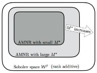
Figure 1 illustrates the relations of these functions and the functional space. The rectangular areas are the classes of functions represented by AMNR with small $M^{*}$, AMNR with large $M^{*}$, and Sobolev space $\mathcal{W}^{\beta}$ with rank additivity.

Figure 1: Functional space and the effect of $M^{*}$.

Note that the formal assumptions and proofs of this section are shown in supplementary material.

4.1 Estimation with Finite $M^{*}$

The consistency of Bayesian nonparametric estimators is evaluated in terms of posterior consistency Ghosal et al. (2000); Ghosal and van der Vaart (2007); van der Vaart and van Zanten (2008). Here, we follow the same strategy. Let $\|f\|_{n}^{2}:=\frac{1}{n}\sum_{i=1}^{n}f(x_{i})^{2}$ be the empirical norm. We define $\epsilon_{n}^{(k)}$ as the contraction rate of the estimator of local function $f^{(k)}$, which evaluates the probability mass of the GP around the true function. Note that the order of $\epsilon_{n}^{(k)}$ depends on the covariance kernel function of the GP prior, in which the optimal rate of $\epsilon_{n}^{(k)}$ is given by (3) with $d=I_{k}$. For brevity, we suppose that the variance of the noise $u_{i}$ is known and the kernel in the GP prior is selected to be optimal. Then, we obtain the following result.

Theorem 1 (Convergence analysis).

Let $M=M^{*}<\infty$. Then, with Assumption 1 and some finite constant $C>0$,

$$E\|\hat{f}_{n}-f^{*}\|_{n}^{2}\leq Cn^{-2\beta/(2\beta+\max_{k}I_{k})}.$$

Theorem 1 claims the validity of the estimator (9). Its convergence rate corresponds to the minimax optimal rate of estimating a function in $\mathcal{W}^{\beta}$ on compact support in $\mathbb{R}^{I_{k}}$, showing that the convergence rate of AMNR depends only on the largest dimensionality of $X$.

4.2 Estimation with Infinite $M^{*}$

When $M^{*}$ is infinite, we cannot use the same strategy used in Section 4.1. Instead, we truncate $M^{*}$ by finite $M$ and evaluate the bias error caused by the truncation. To evaluate the bias, we assume that the local functions are in descending order of their volumes $\bar{f}_{m}:=\sum_{r}\prod_{k}f_{m}^{(k)}$, i.e., $\{\bar{f}_{m}\}$ are ordered as satisfying $\|\bar{f}_{m^{\prime}}\|_{2}\geq\|\bar{f}_{m}\|_{2}$ for all $m^{\prime}>m$. We then introduce the assumption that $\|\bar{f}_{m}\|$ decays to zero polynomially with respect to $m$.

Assumption 1.

With some constant $\gamma>0$,

$$\|\bar{f}_{m}\|_{2}=O\left(m^{-\gamma}\right),$$

as $m\rightarrow\infty$.

This assumption is sufficiently limited. For example, if we pick $\{f^{(k)}_{m}\}$ as $\sum_{r}\prod_{k=1}^{K}f_{m}^{(k)}(x_{r}^{(k)})$ are orthogonal to each $m$, then the Parseval-type inequality leads to $\sum_{m}\|\bar{f}_{m}\|_{2}=\|\sum_{m}\bar{f}_{m}\|_{2}=\|f^{*}\|_{2}<\infty$, implying $\|\bar{f}_{m}\|_{2}\to 0$ as $m\to\infty$.

Then we claim the main result in this section.

Theorem 2.

Suppose we construct the estimator (9) with

$$M\asymp(n^{-2\beta/(2\beta+\max_{k}I_{k})})^{\gamma/(1+\gamma)},$$

where $\asymp$ denotes equality up to a constant. Then, with some finite constant $C>0$,

$$E\|\hat{f}_{n}-f^{*}\|_{n}^{2}\leq C(n^{-2\beta/(2\beta+\max_{k}I_{k})})^{\gamma/(1+\gamma)}.$$

The above theorem states that, even if we truncate $M^{*}$ by finite $M$, the convergence rate is nearly the same as the case of finite $M^{*}$ (Theorem 1), which is slightly worsened by the factor $\gamma/(1+\gamma)$.

Theorem 2 also suggests how to determine $M$. For example, if $\gamma=2,\beta=1$, and $\max_{k}I_{k}=100$, $M\asymp n^{1/70}$ is recommended, which is much smaller than the sample size. Our experimental results (Section 6.3) also support this. Practically, very small $M$ is sufficient, such as $1$ or $2$, even if $n$ is greater than $300$.

Here, we show the conditional consistency of AMNR, which is directly derived from Theorem 2.

Corollary 1.

For all function $f^{*}\in\mathcal{W}^{\beta}$ with finite $M=M^{*}$ or Assumption 1, the estimator (9) satisfies

$$E\|\hat{f}_{n}-f^{0}\|_{n}^{2}\rightarrow 0,$$

as $n\rightarrow\infty$.

5 Related Work

5.1 Nonparametric Tensor Regression

The tensor GP (TGP) (Zhao et al., 2014; Hou et al., 2015) in a method that estimates the function in $\mathcal{W}^{\beta}(\mathcal{S})$ directly. TGP is essentially a GP regression model that flattens a tensor into a high-dimensional vector and takes the vector as an input. Zhao et al. (2014) proposed its estimator and applied it to image recognition from a monitoring camera. Hou et al. (2015) applied the method to analyze brain signals. Although both studies demonstrated the high performance of TGP, its theoretical aspects such as convergence have not been discussed.

Signoretto et al. (2013) proposed a regression model with tensor product reproducing kernel Hilbert spaces (TP-RKHSs). Given a set of vectors $\{x_{k}\}_{k=1}^{K}$, their model is written as

$$\sum_{j}\alpha_{j}\prod_{k}f_{j}^{(k)}(x_{k}),$$ (11)

where $\alpha_{j}$ is a weight. The key difference between TP-RKHSs (11) and AMNR is in the input. TP-RKHSs take only a single vector for each order, meaning that the input is implicitly assumed as rank one. On the other hand, AMNR takes rank-$R$ tensors where $R$ can be greater than one. This difference allows AMNR to be used for more general purposes, because the tensor rank observed in the real world is mostly greater than one. Furthermore, the properties of the estimator, such as convergence, have not been investigated.

5.2 TLR

For the matrix case ($K=2$), Dyrholm et al. (2007) proposed a classification model as (2), where $B$ is assumed to be low rank. Hung and Wang (2013) proposed a logistic regression where the expectation is given by (2) and $B$ is a rank-one matrix. Zhou et al. (2013) extended these concepts for tensor inputs. Suzuki (2015) and Guhaniyogi et al. (2015) proposed a Bayes estimator of TLR and investigated its convergence rate.

Interestingly, AMNR is interpretable as a piecewise nonparametrization of TLR. Suppose $B$ and $X$ have rank-$M$ and rank-$R$ CP decompositions, respectively. The inner product in the tensor space in (2) is then rewritten as the product of the inner product in the low-dimensional vector space, i.e.,

$$\langle B,X_{i}\rangle=\sum_{m=1}^{M}\sum_{r=1}^{R}\lambda_{r,i}\prod_{k=1}^{K}\langle b_{m}^{(k)},x_{r,i}^{(k)}\rangle,$$ (12)

where $b_{m}^{(k)}$ is the order-$K$ decomposed vector of $B$. The AMNR formation is obtained by replacing the inner product $\langle b_{m}^{(k)},x_{r}^{(k)}\rangle$ with local function $f_{m}^{(k)}$.

From this perspective, we see that AMNR incorporates the advantages of TLR and TGP. AMNR captures nonlinear relations between $Y$ and $X$ through $f_{m}^{(k)}$, which is impossible for TLR due to its linearity. Nevertheless, in contrast to TGP, an input of the function constructed in a nonparametric way is given by an $I_{k}$-dimensional vector rather than an $(I_{1},\dots,I_{K})$-dimensional tensor. This reduces the dimension of the function’s support and significantly improves the convergence rate (Section 4).

5.3 Other studies

Koltchinskii et al. (2010) and Suzuki et al. (2013) investigated Multiple Kernel Learning (MKL) considering a nonparametric $p$-variate regression model with an additive structure: $\sum_{j=1}^{p}f_{j}(x_{j})$. To handle high dimensional inputs, MKL reduces the input dimensionality by the additive structure for $f_{j}$ and $x_{j}$. Note that both studies deal with a vector input, and they do not fit to tensor regression analysis.

Table 1: Comparison of related methods.

l Method	Tensor Input	Non- linearity	Convergence Rate with (3)
TLR	$\surd$		$d=0$
TGP	$\surd$	$\surd$	$d=\prod_{k}I_{k}$
TP-RKHSs	rank-$1$	$\surd$	N/A
MKL		$\surd$	N/A
AMNR	$\surd$	$\surd$	$d=\max I_{k}$

Table 1 summarizes the methods introduced in this section. As shown, MKL and TP-RKHSs are not applicable for general tensor input. In contrast, TLR, TGP, and AMNR can take multi-rank tensor data as inputs, and their applicability is much wider. Among the three methods, AMNR is only the one that manages nonlinearity and avoids the curse of dimensionality on tensors.

(a) Full view

(b) Enlarged view

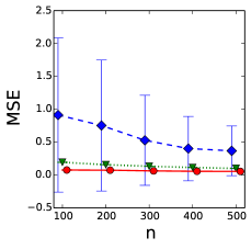
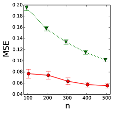
Figure 2: Synthetic data experiment: Low-rank data.

(a) Full view

(b) Enlarged view

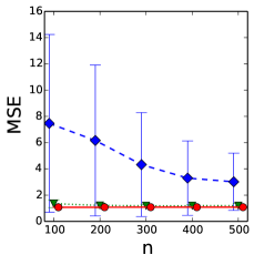
Figure 3: Synthetic data experiment: Full-rank data.

(a) Full view

(b) Enlarged view

Figure 4: Synthetic data experiment: Sensitivity of $R$.

Figure 5: Synthetic data experiment: Sensitivity of $M$.

6 Experiments

6.1 Synthetic Data

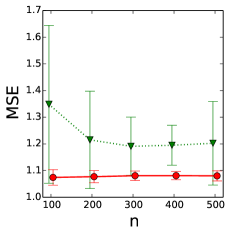
We compare the prediction performance of three models: TLR, TGP, and AMNR. In all experiments, we generate datasets by the data generating process (dgp) as $Y=f^{*}(X)+u$ and fix the noise variance as $\sigma^{2}=1$. We set the size of $X\in\mathbb{R}^{20\times 20}$, i.e., $K=2$ and $I_{1}=I_{2}=20$. By varying the sample size as $n\in\{100,200,300,400,500\}$, we evaluate the empirical risks by the mean-squared-error (MSE) for the testing data, for which we use one-half of the samples. For each experiment, we derive the mean and variance of the MSEs in 100 trials. For TGP and AMNR, we optimize the bandwidth of the kernel function by grid search in the training phase.

6.1.1 Low-Rank Data

First, we consider the case that $X$ and the dgp are exactly low rank. We set $R^{*}$, the true rank of $X$, as $R^{*}=4$ and

$$f^{*}(X)=\sum_{r=1}^{R^{*}}\lambda_{r}\prod_{k=1}^{K}(1+\exp(–\gamma^{T}x_{r}^{(k)}))^{-1}$$

where $[\gamma]_{j}=0.1j$. The results (Figure 3) show that AMNR and TGP clearly outperform TLR, implying that they successfully capture the nonlinearity of the true function. To closely examine the difference between AMNR and TGP, we enlarge the corresponding part (Figure 3(b)), which shows that AMNR consistently outperforms TGP. Note that the performance of TGP improves gradually as $n$ increases, implying that the sample size is insufficient for TGP due to its slow convergence rate.

6.1.2 Full-Rank Data

Next, we consider the case that $X$ is full rank and the dgp has no low-rank structure, i.e., model misspecification will occur in TLR and AMNR. We generate $X$ as $X_{j_{1}j_{2}}\sim\mathcal{N}(0,1)$ with

$$f^{*}(X)=\prod_{k=1}^{K}(1+\exp(-\|X\|_{2}/\prod_{k}I_{k}))^{-1}.$$

The results (Figure 3) show that, as in the previous experiment, AMNR and TGP outperform TLR. Although the difference between AMNR and TGP (Figure 3(b)) is much smaller, AMNR still outperforms TGP. This implies that, while the effect of AMNR’s model misspecification is not negligible, TGP’s slow convergence rate is more problematic.

6.2 Sensitivity of Hyperparameters

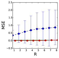
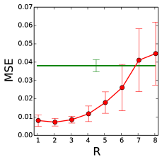
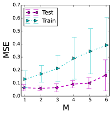
Here, we investigate how the truncation of $R^{*}$ and $M^{*}$ affect prediction performance. In the following experiments, we fix the sample size as $n=300$.

First, we investigate the sensitivity of $R$. We use the same low-rank dgp used in Section 6.1.1 (i.e., $R^{*}=4$.) The results (Figure 5) show that AMNR and TGP clearly outperform TLR. Although their performance is close, AMNR beats TGP when $R$ is not too large, implying that the negative effect of truncating $R^{*}$ is limited.

Next, we investigate the sensitivity of $M$. We use the same full-rank dgp used in Section 6.1.2. Figure 5 compares the training and testing MSEs of AMNR, showing that both errors increase as $M$ increases. These results imply that the model bias decreases quickly and estimation error is more dominant. Indeed, the lowest testing MSE is achieved at $M=2$. This agrees satisfactory with the analysis in Section 4.2, which recommends small $M$.

6.3 Convergence Rate

Here, we confirm how the empirical convergence rates of AMNR and TGP meet the theoretical convergence rates. To clarify the relation, we generate synthetic data from dgp with $\beta=1$ such that the difference between TGP and AMNR is maximized. To do so, we design the dgp function as $f^{*}(X)=\sum_{r=1}^{R}\prod_{k=1}^{K}f^{(k)}(x_{r}^{(k)})$ and

$$f^{(k)}=\sum_{l}\mu_{l}\phi_{l}(\gamma^{T}x),$$

where $\phi_{l}(z)=\sqrt{2}\cos((l-1/2)\pi z)$ is an orthonormal basis function of the functional space and $\mu_{l}=l^{-3/2}\sin(l)$.

Setting	$K$	$R^{*}$	$I_{1}$	$I_{2}$	$I_{3}$	$d$ in (3)
No.						TGP	AMNR
(i)	$3$	$2$	$10$	$10$	$10$	$1000$	$10$
(ii)	$3$	$2$	$3$	$3$	$3$	$27$	$3$
(iii)	$3$	$2$	$10$	$3$	$3$	$90$	$10$

Table 2: Synthetic data experiment: Settings for convergence rate.

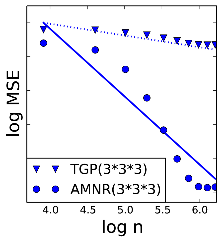
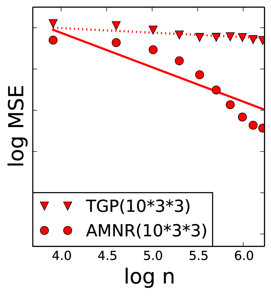
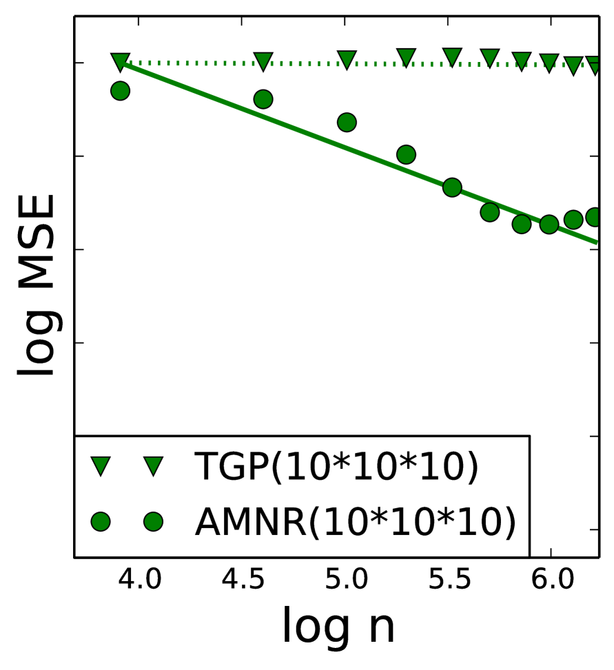
For $X$ we consider three variations: $3\times 3\times 3$, $10\times,3\times 3$, and $10\times 10\times 10$ (Table 2). Figure 6 shows testing MSEs averaged over $100$ trials. The theoretical convergence rates are also depicted by the dashed line (TGP) and the solid line (AMNR). To align the theoretical and empirical rates, we adjust them at $n=50$. The result demonstrates the theoretical rates agree with the practical performance.

(I) $10\times 10\times 10$ tensor.

(II) $3\times 3\times 3$

tensor.

(III) $10\times 3\times 3$ tensor.

Figure 6: Comparison of convergence rate.

6.4 Prediction of Epidemic Spreading

Here, we deal with the epidemic spreading problem in complex networks Anderson and May (1991); Vespignani (2012) as a matrix regression problem. More precisely, given an adjacency matrix network $X_{i}$, we simulate the spreading process of a disease by the susceptible-infected-recovered (SIR) model as follows.

1. We select 10 nodes as the initially infected nodes.

2. The nodes adjacent to the infected nodes become infected with probability $0.01$.

3. Repeat Step 2. After 10 epochs, the infected nodes recover and are no longer infected (one iteration = one epoch).

After the convergence of the above process, we count the total number of infected nodes as $Y_{i}$. Note that the number of infected nodes depends strongly on the network structure and its prediction is not trivial. Conducting the simulation is of course a reliable approach; however, it is time-consuming, especially for large-scale networks. In contrast, once we obtain a trained model, regression methods make prediction very quick.

As a real network, we use the Enron email dataset Klimt and Yang (2004), which is a collection of emails. We consider these emails as undirected links between senders and recipients (i.e., this is a problem of estimating the number of email addresses infected by an email virus). First, to reduce the network size, we select the top $1,000$ email addresses based on frequency and delete emails sent to and received from other addresses. After sorting the remaining emails by timestamp, we sequentially construct an adjacency matrix from every $2,000$ emails, and we finally obtain $220$ input matrices.

For the analysis, we set $R=2$ for the AMNR and TLR methods. Although $R=2$ seems small, we can still use the top-two eigenvalues and eigenvectors, which contain a large amount of information about the original tensor. In addition, the top eigenvectors are closely related to the threshold of outbreaks in infection networks Wang et al. (2003). From these perspectives, the good performance demonstrated by AMNR with $R=2$ is reasonable. The bandwidth of the kernel is optimized by grid search in the training phase.

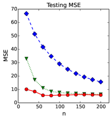
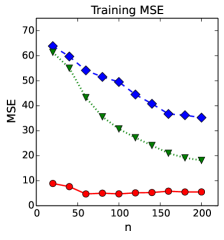
Figure 7 shows the training and testing MSEs. Firstly, there is a huge performance gap between TLR and the nonparametric models in the testing error. This indicates that the relation between epidemic spreading and a graph structure is nonlinear and the linear model is deficient for this problem. Secondly, AMNR outperforms TGP for every $n$ in both training and testing errors. In addition, the performance of AMNR is constantly good and almost unaffected by $n$. This suggests that the problem has some extrinsic information that inflates the dimensionality, and the efficiency of TGP is diminished. On the other hand, it seems AMNR successfully captures the intrinsic information in a low-dimensional space by its “double decomposition” so that AMNR achieves the low-bias and low-variance estimation.

Figure 7: Epidemic spreading experiment: Prediction performance.

7 Conclusion and Discussion

We have proposed AMNR, a new nonparametric model for the tensor regression problem. We constructed the regression function as the sum-product of the local functions, and developed an estimation method of AMNR. We have verified our theoretical analysis and demonstrated that AMNR was the most accurate method for predicting the spread of an epidemic in a real network.

The most important limitation of AMNR is the computational complexity, which is better than TGP but worse than TLR. The time complexity of AMNR with the GP estimator is $O(nR\prod_{k}I_{k}+M(nR)^{3}\sum_{k}I_{k})$, where CP decomposition requires $O(R\prod_{k}I_{k})$ Phan et al. (2013) for $n$ inputs and the GP prior requires $O(I_{k}(nR)^{3})$ for the $MK$ local functions. On the contrary, TGP requires $O(n^{3}\prod_{k}I_{k})$ computation because it must evaluate all the elements of $X$ to construct the kernel Gram matrix. When $R\ll n^{2}$ and $MR^{3}\sum_{k}I_{k}\ll\prod_{k}I_{k}$, which are satisfied in many practical situations, the proposed method is more efficient than TGP.

Approximation methods for GP regression can be used to reduce the computational burden of AMNR. For example, Williams and Seeger (2001) proposed the Nyström method, which approximates the kernel Gram matrix by a low-rank matrix. If we apply rank-$L$ approximation, the computational cost of AMNR can be reduced to $O((L^{3}+nL^{2})\prod_{k}I_{k})$.

Appendix A Proof of Theorem 1

Here, we describe the detail and proof of Theorem 1. At the beginning, we introduce a general theory for evaluating the convergence of a Bayesian estimator.

Preliminary, we introduce some theorems from previous studies. Let $P_{0}$ be a true distribution of $X$, $K(f,g)$ be the Kullback-Leibler divergence, and define $V(f,g)=\int(\log(f/g))^{2}fdx$. Let $d$ be the Hellinger distance, $N(\epsilon,\mathcal{P},d)$ be the bracketing number, and $D(\epsilon,\mathcal{P},d)$ be the packing number. Also we consider a reproducing kernel Hilbert space (RKHS), which is a closure of linear space spanned by a kernel function. Denote by $\mathcal{H}^{(k)}$ the RKHS on $\mathcal{X}^{(k)}$.

The following theorem provides a novel tool to evaluate the Bayesian estimator by posterior contraction.

Theorem 3 (Theorem 2.1 in Ghosal et al. (2000)).

Consider a posterior distribution $\Pi_{n}(\cdot|D_{n})$ on a set $\mathcal{P}$. Let $\epsilon_{n}$ be a sequence such that $\epsilon_{n}\rightarrow 0$ and $n\epsilon_{n}^{2}\rightarrow\infty$. Suppose that, for a constant $C>0$ and sets $\mathcal{P}_{n}\subset\mathcal{P}$, we have

1. $\log D(\epsilon_{n},\mathcal{P}_{n},d)\leq n\epsilon_{n}^{2}$,

2. $\Pi_{n}(\mathcal{P}_{n}\backslash\mathcal{P})\leq\exp(-n\epsilon_{n}^{2}(C+4))$,

3. $\Pi_{n}\left(p:-K(p,p_{0})\leq\epsilon_{n}^{2},V(p,p_{0})\leq\epsilon_{n}^{2}\right)\geq\exp(-Cn\epsilon_{n}^{2})$.

Then, for sufficiently large $C^{\prime}$, $E\Pi_{n}(P:d(P,P_{0})\geq C^{\prime}\epsilon_{n})|D_{n})\rightarrow 0$.

Based on the theorem, van der Vaart and van Zanten (2008) provide a more useful result for the Bayesian estimator with the GP prior. They consider the estimator for an infinite dimensional parameter with the GP prior and investigated the posterior contraction of the estimator with GP. They provide the following conditions.

Condition (A)

With some Banach space $(\mathcal{B},\|\cdot\|)$ and RKHS $(\mathcal{H},\|\cdot\|)$,

1. $\log N(\epsilon_{n},B_{n},\|\cdot\|)\leq Cn\epsilon_{n}^{2}$,

2. $\mbox{Pr}(W\notin B_{n})\leq\exp(-Cn\epsilon_{n}^{2})$,

3. $\mbox{Pr}\left(\|W-w_{0}\|<2\epsilon_{n}\right)\geq\exp(-Cn\epsilon_{n}^{2})$,

where $W$ is a random element in $\mathcal{B}$ and $w_{0}$ is a true function in support of $W$.

When the estimator with the GP prior satisfied the above conditions, the posterior contraction of the estimator is obtained as Theorem 2.1 in Ghosal et al. (2000).

Based on this, we obtain the following result. Consider a set of GP $\{\{W_{m,x}^{(k)}:x\in\mathcal{X}^{(k)}\}\}_{m=1,\ldots,M,k=1,\ldots,K}$ and let $\{F_{x}:x\in\mathcal{X}\}$ be a stochastic process that satisfies $F_{x}=\sum_{m}\sum_{r}\lambda_{r}\prod_{k}W_{m,x_{r}^{(k)}}^{(k)}$.

Also we assume that there exists a true function $f_{0}$ which is constituted by a unique set of local functions $\{w_{m,0}^{(k)}\}_{m=1,\ldots,M,k=1,\ldots,K}$.

To describe posterior contraction, we define a contraction rate $\epsilon_{n}^{(k)}$. It converges to zero as $n\rightarrow\infty$. Let $\phi^{(k)}(\epsilon)$ be a concentration function such that

$$\phi^{(k)}(\epsilon):=\inf_{h\in\mathcal{H}^{(k)}:\|h-w_{0}\|<\epsilon}\|h\|_{\mathcal{H}^{(k)}}^{2}-\log\mbox{Pr}(\|W^{(k)}\|<\epsilon),$$

where $\|\cdot\|_{\mathcal{H}^{(k)}}$ is the norm induced by the inner product of RKHS. We define the contraction rate with $\phi^{(k)}(\epsilon)$. We denote a sequence $\{\epsilon_{n}^{(k)}\}_{n,k}$ satisfying

$$\phi^{(k)}(\epsilon_{n}^{(k)})\leq n(\epsilon_{n}^{(k)})^{2}.$$

The order of $\epsilon_{n}^{(k)}$ depends on a choice of kernel function, where the optimal minimax rate is $\epsilon_{n}^{(k)}=O(n^{-\beta_{k}/(\beta_{k}+I_{k})})$ Tsybakov (2008). In the following part, we set $\tilde{\epsilon_{n}}^{(k)}=\tilde{\epsilon}_{n}$ for every $k$. As $k^{\prime}=\arg\max_{k}I_{k}$, the $\epsilon_{n}^{(k)}$ satisfies the condition about the concentration function.

We also note the relation between posterior contraction and the well-known risk bound. Suppose the posterior contraction such that $E\Pi_{n}(\theta:d_{n}^{2}(\theta,\theta_{0})\geq C\epsilon_{n}^{2}|D_{n})\rightarrow 0$ holds, where $\theta$ is a parameter, $\theta_{0}$ is a true value, and $d_{n}$ is a bounded metric. Then we obtain the following inequality:

$$E\Pi_{n}(d_{n}^{2}(\theta,\theta_{0})|D_{n})\leq C\epsilon_{n}^{2}+DE\Pi_{n}(\theta:d_{n}^{2}(\theta,\theta_{0})\geq C\epsilon_{n}^{2}|D_{n}),$$

where $D$ is a bound of $d_{n}$. This leads $E\Pi_{n}(d_{n}^{2}(\theta,\theta_{0})|D_{n})=O(C\epsilon_{n}^{2})$. In addition, if $\theta\mapsto d_{n}^{2}(\theta,\theta_{0})$ is convex, the Jensen’s inequality provides $d_{n}^{2}(\theta,\theta_{0})\leq\Pi_{n}(d_{n}^{2}(\theta,\theta_{0})|D_{n})$. By taking the expectation, we obtain

$$Ed_{n}^{2}(\theta,\theta_{0})\leq E\Pi_{n}(d_{n}^{2}(\theta,\theta_{0})|D_{n})=O(C\epsilon_{n}^{2}).$$

We start to prove Theorem 1. First, we provide a lemma for functional decomposition. When the function has a form of a $k$-product of local functions, we bound a distance between two functions with a $k$-sum of distance by the local functions.

Lemma 1.

Suppose that two functions $f,g:\times_{k=1}^{K}\mathcal{X}_{k}\rightarrow\mathbb{R}$ have a form $f=\prod_{k}f_{k}$ and $g=\prod_{k}g_{k}$ with local functions $f_{k},g_{k}:\mathcal{X}_{k}\rightarrow\mathbb{R}$. Then we have a bound such that

$$\left\|f-g\right\|\leq\sum_{k}\left\|f_{k}-g_{k}\right\|\max\left\{\left\|f_{k}\right\|,\left\|g_{k}\right\|\right\}.$$

Proof.

We show the result based on induction. When $k=2$, we have

$$f-g=f_{1}f_{2}-g_{1}g_{2}=f_{1}(f_{2}-g_{2})+(f_{1}-g_{1})g_{2},$$

and

$$\left\|f-g\right\|\leq\left\|f_{1}\right\|\left\|f_{2}-g_{2}\right\|+\left\|f_{1}-g_{1}\right\|\left\|g_{2}\right\|.$$

Thus the result holds when $k=2$.

Assume the result holds when $k=k^{\prime}$. Let $k=k^{\prime}+1$. The difference between $k^{\prime}+1$-product functions is written as

$$f-g=f_{k^{\prime}+1}\prod_{k^{\prime}}f_{k}-g_{k^{\prime}+1}\prod_{k^{\prime}}g_{k}=\prod_{k^{\prime}}f_{k}(f_{k^{\prime}+1}-g_{k^{\prime}+1})+(\prod_{k^{\prime}}f_{k}-\prod_{k^{\prime}}g_{k})g_{k^{\prime}+1}.$$

From this, we obtain the bound

$$\left\|f-g\right\|\leq\left\|\prod_{k^{\prime}}f_{k}\right\|\left\|f_{k^{\prime}+1}-g_{k^{\prime}+1}\right\|+\left\|\prod_{k^{\prime}}f_{k}-\prod_{k^{\prime}}g_{k}\right\|\left\|g_{k^{\prime}+1}\right\|.$$

The distance $\left\|\prod_{k^{\prime}}f_{k}-\prod_{k^{\prime}}g_{k}\right\|$ is decomposed recursively by the case of $k=k^{\prime}$. Then we obtain the result. ∎

Now we provide the proof of Theorem 1. Note that $M=M^{*}<\infty$ in the statement in Theorem 1. Asume that $C,C^{\prime},C^{\prime\prime},\ldots$ are some positive finite constants and they are not affected by other values.

Proof.

We will show that $F_{x}$ satisfies the condition (A). Firstly, we check the third condition in the theorem.

According to Lemma 1, the value $\|F_{x}-f_{0}\|$ is bounded as

$$\|F_{x}-f_{0}\| \leq\sum_{m}\sum_{r}\left\|\prod_{k}W_{r}^{(k)}-\prod_{k}w_{m,0}^{(k)}\right\|$$

$$\leq\sum_{m}\sum_{r}\sum_{k}\left\|W_{m}^{(k)}-w_{m,0}^{(k)}\right\|\prod_{k^{\prime}\neq k}\max\left\{\left\|w_{m,0}^{(k^{\prime})}\right\|,\left\|W_{m}^{(k^{\prime})}\right\|\right\}.$$

By denoting $\left\|\tilde{W}_{m}^{(k^{\prime})}\right\|:=\max\left\{\left\|w_{m,0}^{(k^{\prime})}\right\|,\left\|W_{m}^{(k^{\prime})}\right\|\right\}$, we evaluate the probability $Pr(\|F-f_{0}\|\leq\epsilon_{n})$ as

$$\mbox{Pr}(\|F-f_{0}\|\leq\epsilon_{n}) \geq\mbox{Pr}\left(\sum_{m}\sum_{r}\sum_{k}\left\|W_{m}^{(k)}-w_{m,0}^{(k)}\right\|\prod_{k^{\prime}\neq k}\left\|\tilde{W}_{m}^{(k^{\prime})}\right\|\leq\epsilon_{n}\right)$$

$$\geq\mbox{Pr}\left(\sum_{r}\sum_{k}\sum_{m}\left\|W_{m}^{(k)}-w_{m,0}^{(k)}\right\|\leq\frac{1}{C_{k}}\epsilon_{n}\right),$$ (13)

where $C_{k}$ is a positive finite constant satisfying $C_{k}=\max_{m}\prod_{k}\left\|\tilde{W}_{m}^{(k^{\prime})}\right\|$.

From van der Vaart and van Zanten (2008), we use the following inequality for every Gaussian random element $W$:

$$\mbox{Pr}\left(\|W-w_{0}\|\leq\epsilon_{n}\right)\geq\exp(-n\epsilon_{n}^{2}),$$

Then, by seting $\epsilon_{n}=\sum_{m,r,k}\epsilon_{n}^{(k)}$ and with some constant $C$, we bound (13) below as

$$\mbox{Pr}\left(\sum_{r}\sum_{k}\sum_{m}\left\|W_{m}^{(k)}-w_{m,0}^{(k)}\right\|\leq\frac{1}{C_{k}}\sum_{m,r,k}\epsilon_{n}^{(k)}\right)$$

$$\geq\prod_{m,r,k}\mbox{Pr}\left(\left\|W_{m}^{(k)}-w_{m,0}^{(k)}\right\|\leq\frac{1}{C_{k}}\epsilon_{n}^{(k)}\right)$$

$$\geq\prod_{m}\prod_{r}\prod_{k}\exp\left(-\frac{n}{\left(C_{k}\right)^{2}}\epsilon_{n}^{(k),2}\right)$$

$$\geq\exp\left(-n\sum_{m,r,k}\epsilon_{n}^{(k),2}\right).$$

For the second condition, we define a subspace of the Banach space as

$$B_{n}^{(k)}=\epsilon_{n}^{(k)}\mathcal{B}_{1}^{(k)}+M_{n}^{(k)}\mathcal{H}_{1}^{(k)},$$

for all $k=1,\ldots,K$. Note $\mathcal{B}_{1}^{(k)}$ and $\mathcal{H}_{1}^{(k)}$ are unit balls in $\mathcal{B}$ and $\mathcal{H}$. Also, we define $B_{n}$ as

$$B_{n}:=\left\{w:w=MR\prod_{k}w_{k},w_{k}\in B_{n}^{(k)},\forall k\right\}.$$

As shown in van der Vaart and van Zanten (2008), for every $r$ and $k$,

$$Pr\left(W_{m}^{(k)}\notin B_{n}^{(k)}\right)\leq 1-\Phi(\alpha_{n}^{(k)}+M_{n}^{(k)}),$$

where $\Phi$ is the cumulative distribution function of the standard Gaussian distribution; $\alpha_{n}^{(k)}$ and $M_{n}^{(k)}$ satisfy the following equation with a constant $C^{\prime}>0$ as

$$\alpha_{n}^{(k)}=\Phi^{-1}(Pr(W_{m}^{(k)}\in\epsilon_{n}\mathcal{B}_{1}^{(k)}))=\Phi^{-1}(\exp(-\phi_{0}(\epsilon_{n}^{(k)}))),$$

$$M_{n}^{(k)}=-2\Phi^{-1}(\exp(-C^{\prime}n(\epsilon_{n}^{(k)})^{2})).$$

By setting $\alpha_{n}^{(k)}+M_{n}^{(k)}\geq\frac{1}{2}M_{n}^{(k)}$ and using the relation $\phi_{0}(\epsilon)\leq n\epsilon_{n}^{2}$, we have

$$Pr\left(W_{m}^{(k)}\notin B_{n}^{(k)}\right)\leq 1-\Phi\left(\frac{1}{2}M_{n}^{(k)}\right)=\exp(-C^{\prime}n(\epsilon_{n}^{(k)})^{2}).$$

This leads

$$Pr(F_{x}\notin B_{n}) \leq\prod_{m}\prod_{k}\prod_{r}\mbox{Pr}(W_{m}^{(k)}\notin B_{n}^{(k)})$$

$$\leq\prod_{m}\prod_{k}\prod_{r}\exp(-C^{\prime}n(\epsilon_{n}^{(k)})^{2})$$

$$=\exp(-C^{\prime}\sum_{m,r,k}(\epsilon_{n}^{(k)})^{2}).$$

Finally, we show the first condition. Let $\{h_{j}^{(k)}\}_{j=1}^{N^{(k)}}$ be a set of elements of $M_{n}^{(k)}\mathcal{H}_{1}^{(k)}$ for all $k$. Also, we set that each $h_{j}^{(k)}$ are $2\epsilon_{n}^{(k)}$ separated, thus $\epsilon_{n}^{(k)}$ balls with center $h_{j}^{(k)}$ do not have intersections. According to Section 5 in van der Vaart and van Zanten (2008), we have

$$1 \geq\sum_{j=1}^{N^{(k)}}\mbox{Pr}(W_{m}^{(k)}\in h_{j}^{(k)}+\epsilon_{n}B_{1}^{(k)})$$

$$\geq\sum_{j=1}^{N^{(k)}}\exp(-\frac{1}{2}\|h_{j}^{(k)}\|_{\mathcal{H}}^{2})Pr(W\in\epsilon_{n}^{(k)}\mathcal{B}_{1}^{(k)})$$

$$\geq N^{(k)}\exp\left(-\frac{1}{2}(M_{n}^{(k)})^{2}\right)\exp(-\phi_{0}(\epsilon_{n}^{(k)})).$$

Consider $2\epsilon_{n}^{(k)}$-nets with center $\{h_{j}^{(k)}\}_{j=1}^{N^{(k)}}$. The nets cover $M_{n}^{(k)}\mathcal{H}_{1}^{(k)}$, we obtain

$$N(2\epsilon_{n}^{(k)},M_{n}^{(k)}\mathcal{H}_{1}^{(k)},\|\cdot\|)\leq N^{(k)}\leq\exp\left(\frac{1}{2}(M_{n}^{(k)})^{2}\right)\exp(\phi^{(k)}(\epsilon_{n}^{(k)})).$$

Because every point in $B_{n}^{(k)}$ is within $\epsilon_{n}^{(k)}$ from some point of $M_{n}\mathcal{H}_{1}^{(k)}$, we have

$$N(3\epsilon_{n}^{(k)},B_{n}^{(k)},\|\cdot\|)\leq N(2\epsilon_{n}^{(k)},M_{n}^{(k)}\mathcal{H}_{1}^{(k)},\|\cdot\|).$$

By Lemma 1, for every elements $w,w^{\prime}\in B_{n}$ constructed as $w=\prod_{k}w^{(k)},w^{(k)}\in B_{n}^{(k)}$, its distance is evaluated as

$$\|w-w^{\prime}\| =\left\|\prod_{k}w_{k}-\prod_{k}w^{\prime}_{k}\right\|$$

$$\leq\sum_{k}\left\|w^{(k)}-w^{\prime(k)}\right\|\prod_{k^{\prime}\neq k}\left\|\tilde{w}^{(k^{\prime})}\right\|$$

$$\leq\prod_{k^{\prime}\neq k}C_{k^{\prime}}\sum_{k}\left\|w^{(k)}-w^{\prime(k)}\right\|.$$ (14)

We consider a set $\{h^{*}:h^{*}=\prod_{k,j}h_{j}^{(k)}\}$, which are the element of $B_{n}$. According to (14), the $C\epsilon_{n}$-net with center $\{h^{*}\}$ will cover $B_{n}$, and its number is equal to $\prod_{k}N(\epsilon_{n},B_{n}^{(k)},\|\cdot\|)$. Let $C\sum_{m,r,k}\epsilon_{n}^{(k)}=:\epsilon_{n}^{\prime}$ and we have

$$\log N(3\epsilon^{\prime}_{n},B_{n},\|\cdot\|) \leq\sum_{m,r,k}\log N(3\epsilon_{n}^{(k)},B_{n}^{(k)},\|\cdot\|)$$

$$\leq\sum_{m,r,k}\log N(2\epsilon^{(k)}_{n},M_{n}^{(k)}\mathcal{H}_{1}^{(k)},\|\cdot\|)$$

$$\leq\sum_{m,r,k}\left(\frac{1}{2}(M_{n}^{(k)})^{2}+\phi^{(k)}(\epsilon^{(k)}_{n})\right)$$

$$\leq\sum_{m,r,k}\left(C^{\prime\prime}n(\epsilon^{(k)}_{n})^{2}+C^{\prime\prime\prime}n(\epsilon_{n}^{(k)})^{2}\right)$$

$$\leq C^{\prime\prime\prime\prime}n\sum_{m,r,k}(\epsilon^{(k)}_{n})^{2}.$$

The last inequality is from the definition of $M_{n}$ and $\phi^{(k)}(\epsilon_{n})$.

We check that the conditions (A) are all satisfied, thus we obtain posterior contraction of the GP estimator with rate $\epsilon^{(k)}_{n}$. Also, according to the connection between posterior contraction and the risk bound, we achieve the result of Theorem 1.

∎

Appendix B Proof of Theorem 2

We define the representation for the true function. Recall the notation $f=\sum_{m}\bar{f}_{m}$. We introduce the notation for the true function $f^{*}$ and the GP estimator $\hat{f}$ as follow:

$$f^{*}=\sum_{m=1}^{\infty}\bar{f}^{*}_{m}$$

$$\hat{f}_{n}=\sum_{m=1}^{M}\hat{\bar{f}}_{m}.$$

We decompose the above two functions as follows:

$$\|f^{*}-\hat{f}\|_{n} =\left\|\sum_{m=1}^{\infty}\bar{f}^{*}_{m}-\sum_{m=1}^{M}\hat{\bar{f}}_{m}\right\|_{n}$$

$$=\left\|\sum_{m=M+1}^{\infty}\bar{f}_{m}^{*}-\sum_{m=1}^{M}(\bar{f}_{m}^{*}-\hat{\bar{f}}_{m})\right\|_{n}$$

$$\leq\left\|\sum_{m=M+1}^{\infty}\bar{f}_{m}^{*}\right\|_{n}+\left\|\sum_{m=1}^{M}(\bar{f}_{m}^{*}-\hat{\bar{f}}_{m})\right\|_{n}.$$ (15)

Consider the first term with Assumption 1. The expectation of the first term of (15) is bounded by

$$E\left\|\sum_{m=M+1}^{\infty}\bar{f}_{m}^{*}\right\|_{n}\leq\sum_{m=M+1}^{\infty}\left\|\bar{f}_{m}^{*}\right\|_{2}$$

$$\leq C\sum_{m=M+1}^{\infty}m^{-\gamma},$$

with finite constant $C$. The exchangeability of the first inequality is guaranteed by the setting of $f^{*}$. Also, the second inequality comes from Assumption 1. Then, the infinite summation of $m^{-\gamma}$ enables us to obtain that the expectation of the first term is $O(M^{-\gamma})$, by using the relation $\sum_{x=C}^{\infty}x^{-r}\asymp C^{-r}$.

About the second term of (15), we consider the estimation for $f^{*}$ with finite $M$. As shown in the proof of Theorem 1, the estimation of $\sum_{m}^{M}\bar{f}_{m}$ is evaluated as

$$E\|\hat{f}-f^{*}\|_{2}=O\left(\sum_{m}^{M}n^{-\frac{\beta}{2\beta+\max_{k}I_{k}}}\right)=O\left(Mn^{-\frac{\beta}{2\beta+\max_{k}I_{k}}}\right).$$

Finally, we obtain the relation

$$E\|f^{*}-\hat{f}\|_{n}=O(M^{-\gamma})+O\left(Mn^{-\frac{\beta}{2\beta+\max_{k}I_{k}}}\right).$$

Then, we allow $M$ to increase as $n$ increases. Let $M\asymp n^{\zeta}$ with positive constant $\zeta$, and simple calculation concludes that $\zeta=(\frac{\beta}{2\beta+\max_{k}I_{k}})/(1+\gamma)$ is optimal. By substituting $\zeta$, we obtain the result.

References

• Anderson and May (1991) Anderson, R. M. and May, R. M. (1991) Infectious diseases of humans, vol. 1, Oxford university press.
• Carroll and Chang (1970) Carroll, J. D. and Chang, J.-J. (1970) Analysis of individual differences in multidimensional scaling via an n-way generalization of “eckart-young” decomposition, Psychometrika, 35, 283–319.
• Dyrholm et al. (2007) Dyrholm, M., Christoforou, C. and Parra, L. C. (2007) Bilinear discriminant component analysis, The Journal of Machine Learning Research, 8, 1097–1111.
• Ghosal et al. (2000) Ghosal, S., Ghosh, J. K. and van der Vaart, A. W. (2000) Convergence rates of posterior distributions, Annals of Statistics, 28, 500–531.
• Ghosal and van der Vaart (2007) Ghosal, S. and van der Vaart, A. (2007) Convergence rates of posterior distributions for noniid observations, The Annals of Statistics, 35, 192–223.
• Guhaniyogi et al. (2015) Guhaniyogi, R., Qamar, S. and Dunson, D. B. (2015) Bayesian tensor regression, arXiv preprint arXiv:1509.06490.
• Hackbusch (2012) Hackbusch, W. (2012) Tensor spaces and numerical tensor calculus, vol. 42, Springer Science & Business Media.
• Harshman (1970) Harshman, R. (1970) Foundations of the parafac procedure: Models and conditions for an “explanatory” multi-modal factor analysis, UCLA Working Papers in Phonetics, 16.
• Hastie and Tibshirani (1990) Hastie, T. J. and Tibshirani, R. J. (1990) Generalized additive models, vol. 43, CRC Press.
• Hou et al. (2015) Hou, M., Wang, Y. and Chaib-draa, B. (2015) Online local gaussian process for tensor-variate regression: Application to fast reconstruction of limb movement from brain signal, in IEEE International Conference on Acoustics, Speech and Signal Processing.
• Hung and Wang (2013) Hung, H. and Wang, C.-C. (2013) Matrix variate logistic regression model with application to EEG data, Biostatistics, 14, 189–202.
• Klimt and Yang (2004) Klimt, B. and Yang, Y. (2004) The enron corpus: A new dataset for email classification research, in Proceedings of 15th European Conference on Machine Learning, Springer Science & Business Media, vol. 15, p. 217.
• Koltchinskii et al. (2010) Koltchinskii, V., Yuan, M. et al. (2010) Sparsity in multiple kernel learning, The Annals of Statistics, 38, 3660–3695.
• Phan et al. (2013) Phan, A.-H., Tichavsky, P. and Cichocki, A. (2013) Fast alternating ls algorithms for high order candecomp/parafac tensor factorizations, IEEE Transactions on Signal Processing, 61, 4834–4846.
• Ravikumar et al. (2009) Ravikumar, P., Lafferty, J., Liu, H. and Wasserman, L. (2009) Sparse additive models, Journal of the Royal Statistical Society: Series B, 71, 1009–1030.
• Signoretto et al. (2013) Signoretto, M., De Lathauwer, L. and Suykens, J. A. (2013) Learning tensors in reproducing kernel hilbert spaces with multilinear spectral penalties, arXiv preprint arXiv:1310.4977.
• Suzuki (2015) Suzuki, T. (2015) Convergence rate of bayesian tensor estimator and its minimax optimality, in Proceedings of The 32nd International Conference on Machine Learning, pp. 1273–1282.
• Suzuki et al. (2013) Suzuki, T., Sugiyama, M. et al. (2013) Fast learning rate of multiple kernel learning: Trade-off between sparsity and smoothness, The Annals of Statistics, 41, 1381–1405.
• Tomioka et al. (2007) Tomioka, R., Aihara, K. and Müller, K.-R. (2007) Logistic regression for single trial eeg classification, in Advances in Neural Information Processing Systems 19, pp. 1377–1384.
• Tsybakov (2008) Tsybakov, A. B. (2008) Introduction to Nonparametric Estimation, Springer Publishing Company, Incorporated, 1st edn.
• van der Vaart and van Zanten (2008) van der Vaart, A. and van Zanten, H. (2008) Rates of contraction of posterior distributions based on gaussian process priors, The Annals of Statistics, 36, 1435–1463.
• Vespignani (2012) Vespignani, A. (2012) Modelling dynamical processes in complex socio-technical systems, Nature Physics, 8, 32–39.
• Wang et al. (2014) Wang, F., Zhang, P., Qian, B., Wang, X. and Davidson, I. (2014) Clinical risk prediction with multilinear sparse logistic regression, in Proceedings of the 20th ACM SIGKDD International Conference on Knowledge Discovery and Data Mining.
• Wang et al. (2003) Wang, Y., Chakrabarti, D., Wang, C. and Faloutsos, C. (2003) Epidemic spreading in real networks: An eigenvalue viewpoint, in Proceedings. 22nd International Symposium on Reliable Distributed Systems, 2003., IEEE, pp. 25–34.
• Williams and Seeger (2001) Williams, C. K. and Seeger, M. (2001) Using the nyström method to speed up kernel machines, in Advances in Neural Information Processing Systems 13, pp. 682–688.
• Zhao et al. (2013) Zhao, Q., Zhang, L. and Cichocki, A. (2013) A tensor-variate gaussian process for classification of multidimensional structured data, in AAAI Conference on Artificial Intelligence.
• Zhao et al. (2014) Zhao, Q., Zhou, G., Zhang, L. and Cichocki, A. (2014) Tensor-variate gaussian processes regression and its application to video surveillance, in Acoustics, Speech and Signal Processing, 2014 IEEE International Conference, IEEE, pp. 1265–1269.
• Zhou et al. (2013) Zhou, H., Li, L. and Zhu, H. (2013) Tensor regression with applications in neuroimaging data analysis, Journal of the American Statistical Association, 108, 540–552.