Enhancing Sparsity of Hermite Polynomial Expansions by Iterative Rotations

Abstract

Compressive sensing has become a powerful addition to uncertainty quantification in recent years. This paper identifies new bases for random variables through linear mappings such that the representation of the quantity of interest is more sparse with new basis functions associated with the new random variables. This sparsity increases both the efficiency and accuracy of the compressive sensing-based uncertainty quantification method. Specifically, we consider rotation-based linear mappings which are determined iteratively for Hermite polynomial expansions. We demonstrate the effectiveness of the new method with applications in solving stochastic partial differential equations and high-dimensional ($\mathcal{O}(100)$) problems.

$\dagger$ The first two authors made equal contributions to this manuscript.

1 Introduction

Uncertainty quantification (UQ) plays an important role in constructing computational models as it helps to understand the influence of uncertainties on the quantity of interest. In this paper, we study parametric uncertainty, which treats some of the parameters as random variables. Let $(\Omega,\mathcal{F},P)$ be a complete probability space, where $\Omega$ is the event space and $P$ is a probability measure on the $\sigma$-field $\mathcal{F}$. We consider a system depending on a $d$-dimensional random vector $\bm{\xi}(\omega)=(\xi_{1}(\omega),\xi_{2}(\omega),\cdots,\xi_{d}(\omega))^{T}$, where $\omega$ is an event in $\Omega$. For simplicity, we denote $\xi_{i}(\omega)$ as $\xi_{i}$. We aim to approximate the quantity of interest $u(\bm{\xi})$ with a generalized polynomial chaos (gPC) expansion [1, 2]:

$$u(\bm{\xi})=\sum_{n=1}^{N}c_{n}\psi_{n}(\bm{\xi})+\varepsilon(\bm{\xi}),$$ (1.1)

where $\varepsilon$ is the truncation error, $N$ is a positive integer, $c_{n}$ are coefficients, $\psi_{n}$ are multivariate polynomials which are orthonormal with respect to the distribution of $\bm{\xi}$:

$$\int_{\mathbb{R}^{d}}\psi_{i}(\bm{\xi})\psi_{j}(\bm{\xi})\rho(\bm{\xi})\mathrm{d}\bm{\xi}=\delta_{ij},$$ (1.2)

where $\rho(\bm{\xi})$ is the probability distribution function (PDF) of $\bm{\xi}$ and $\delta_{ij}$ is the Kronecker delta. The approximation converges in the $L_{2}$ sense as $N$ increases if $u$ is in the Hilbert space associated with the measure of $\bm{\xi}$ (i.e., the weight of the inner product is the PDF of $\bm{\xi}$) [2, 3, 4]. Stochastic Galerkin and probabilistic collocation are two popular methods [1, 2, 5, 6, 7, 8] used to approximate the gPC coefficients $\bm{c}=(c_{1},c_{2},\cdots,c_{N})^{T}$. Stochastic collocation starts by generating samples of input $\bm{\xi}^{q},q=1,2,\cdots,M$ based on $\rho(\bm{\xi})$. Next, the computational model is calculated for each $\bm{\xi}^{q}$ to obtain corresponding samples of the output $u^{q}=u(\bm{\xi}^{q})$. Finally, $\bm{c}$ are approximated based on $u^{q}$ and $\bm{\xi}^{q}$. Note that in many practical problems, it is very costly to obtain $u^{q}$ and, due to the limited computational sources, we will often have $M<N$ or even $M\ll N$. The smaller number of samples than basis functions implies that the following linear system is under-determined:

$$\mathsfsl{\Psi}\bm{c}=\bm{u}+\bm{\varepsilon},$$ (1.3)

where $\bm{u}=(u^{1},u^{2},\cdots,u^{M})^{T}$ is the vector of output samples, $\mathsfsl{\Psi}$ is an $M\times N$ matrix with $\Psi_{ij}=\psi_{j}(\bm{\xi}^{i})$ and $\bm{\varepsilon}=(\varepsilon^{1},\varepsilon^{2},\cdots,\varepsilon^{M})^{T}$ is a vector of error samples with $\varepsilon^{q}=\varepsilon(\bm{\xi}^{q})$. The compressive sensing method is effective at solving this type of under-determined problem when $\bm{c}$ is sparse [9, 10, 11, 12] and recent studies have applied this approach to uncertainty quantification (UQ) problems [13, 14, 15, 16, 17, 18, 19, 20, 21, 22, 23, 24].

Several useful approaches have been developed to enhance the efficiency of solving Eq. (1.3) in UQ applications. First, re-weighted $\ell_{1}$ minimization assigns a weight to each $c_{n}$ and solves a weighted $\ell_{1}$ minimization problem to enhance the sparsity [25]. The weights can be estimated in a priori [18, 26] or, for more general cases, can be obtained iteratively [15, 17]. Second, better sampling strategies can be used, such as minimizing the mutual coherence [27, 20]. Third, Bayesian compressive sensing method provides the posterior distribution of the coefficients [23, 16]. Finally, adaptive basis selection selects basis functions to enhance the efficiency instead of fixing the basis functions at the beginning [22]. Recently, we propose an approach [17] to enhance the sparsity of $\bm{c}$ through the rotation of the random vector $\bm{\xi}$ to a new random vector $\bm{\eta}$, where the rotation operator is determined by the sorted variability directions of the quantity of interest $u$ based on the active subspace method [28].

In this work, we aim to extend our previous work [17] and consider the specific case where the system depends on i.i.d. Gaussian random variables; i.e., $\bm{\xi}\sim\mathcal{N}(\bm{0},\mathsfsl{I})$ where $\bm{0}$ is a $d$-dimensional zero vector and $\mathsfsl{I}$ is a $d\times d$ identity matrix. This assumption appears in a wide range of physics and engineering problems. We aim to find a mapping $g:\mathbb{R}^{d}\mapsto\mathbb{R}^{d}$ which maps $\bm{\xi}$ to a new set of i.i.d. Gaussian random variables $\bm{\eta}=(\eta_{1},\eta_{2},\cdots,\eta_{d})^{T}$ such that the gPC expansion of $u$ with respect to $\bm{\eta}$ is sparser. In other words,

$$u(\bm{\xi})\approx\sum_{n=1}^{N}c_{n}\psi_{n}(\bm{\xi})=\sum_{n=1}^{N}\tilde{c}_{n}\tilde{\psi}_{n}(\bm{\eta}(\bm{\xi}))\approx u(\bm{\eta}(\bm{\xi})),$$ (1.4)

where $\tilde{\psi}_{n}$ are orthonormal polynomials associated with the new random vector $\bm{\eta}$ and $\tilde{c}_{n}$ are the corresponding coefficients. Note that $\psi_{n}=\tilde{\psi}_{n}$ since $\bm{\eta}\sim\mathcal{N}(\bm{0},\mathsfsl{I})$. We intend to find the set $\tilde{\bm{c}}=(\tilde{c}_{1},\tilde{c}_{2},\cdots,\tilde{c}_{N})^{T}$ which is sparser than $\bm{c}$ while preserving the properties of matrix $\tilde{\mathsfsl{\Psi}}$ (with $\tilde{\Psi}_{ij}=\tilde{\psi}_{j}(\bm{\eta}^{i})$) close to those of $\mathsfsl{\Psi}$ to improve the efficiency of the compressive sensing method. To accomplish this, we will use a linear mapping, based on the idea of active subspaces [28], to obtain $\bm{\eta}$ as first proposed in [17]. Unlike our previous work, we build this mapping iteratively in order to obtain a sparser $\tilde{\bm{c}}$ and improve the efficiency of the gPC approximation by compressive sensing. We also provide the analytical form of the “gradient matrix” (see Eq.(3.3)) to avoid estimating it with Monte Carlo methods. Our method is applicable for both $\ell_{0}$ and $\ell_{1}$ minimization problems. Especially, for the latter, we can also integrate the present method with re-weighted $\ell_{1}$ minimization method to further reduce the error. We demonstrate that, compared with the standard compressive sensing methods, our approach reduces the relative $L_{2}$ error of the gPC approximation.

2 Brief review of the compressive sensing-based gPC method

2.1 Hermite polynomial chaos expansions

In this paper we study systems relying on $d$-dimensional Gaussian random vector $\bm{\xi}\sim\mathcal{N}(\bm{0},\mathsfsl{I})$. Therefore, the gPC basis functions are constructed by tensor products of univariate orthonormal Hermite polynomials. For a multi-index $\bm{\alpha}=(\alpha_{1},\alpha_{2},\cdots,\alpha_{d}),\alpha_{i}\in\mathbb{N}\cup\{0\}$, we set

$$\psi_{\bm{\alpha}}(\bm{\xi})=\psi_{\alpha_{1}}(\xi_{1})\psi_{\alpha_{2}}(\xi_{2})\cdots\psi_{\alpha_{d}}(\xi_{d}).$$ (2.1)

For two different multi-indices $\bm{\alpha}_{i}=((\alpha_{i})_{{}_{1}},(\alpha_{i})_{{}_{2}},\cdots,(\alpha_{i})_{{}_{d}})$ and $\bm{\alpha}_{j}=((\alpha_{j})_{{}_{1}},(\alpha_{j})_{{}_{2}},\cdots,(\alpha_{j})_{{}_{d}})$, we have the property

$$\int_{\mathbb{R}^{d}}\psi_{\bm{\alpha}_{i}}(\bm{\xi})\psi_{\bm{\alpha}_{j}}(\bm{\xi})\rho(\bm{\xi})\mathrm{d}\xi=\delta_{\bm{\alpha}_{i}\bm{\alpha}_{j}}=\delta_{(\alpha_{i})_{{}_{1}}(\alpha_{j})_{{}_{1}}}\delta_{(\alpha_{i})_{{}_{2}}(\alpha_{j})_{{}_{2}}}\cdots\delta_{(\alpha_{i})_{{}_{d}}(\alpha_{j})_{{}_{d}}},$$ (2.2)

where

$$\rho(\bm{\xi})=\left(\dfrac{1}{\sqrt{2\pi}}\right)^{d}\exp\left(-\dfrac{\xi_{1}^{2}+\xi_{2}^{2}+\cdots+\xi_{d}^{2}}{2}\right).$$ (2.3)

For simplicity, we denote $\psi_{\bm{\alpha}_{i}}(\bm{\xi})$ as $\psi_{i}(\bm{\xi})$.

2.2 Compressive sensing

The vector $\bm{c}$ in Eq. (1.3) can be approximated by solving the following optimization problem:

$$(P_{h,\epsilon}):~{}\arg\min_{\hat{\bm{c}}}\|\hat{\bm{c}}\|_{h},\text{~{}~{}subject to~{}~{}}\|\mathsfsl{\Psi}\hat{\bm{c}}-\bm{u}\|_{2}\leq\epsilon,$$ (2.4)

where $\epsilon=\|\bm{\varepsilon}\|_{2}$ and $h$ is typically set as $0$ or $1$. For $h=0$ ($\ell_{0}$ minimization problem), the greedy Orthogonal Matching Pursuit (OMP) algorithm [29, 12] can be applied; for $h=1$ ($\ell_{1}$ minimization problem), convex optimization methods are directly applicable [30]. As pointed out in [12], OMP is very efficient – when it works – but convergence to a sparse solution is not always guaranteed. There are specific cases where a sparse solution is possible while OMP yields a dense one. Since both the OMP and $\ell_{1}$ minimization approaches are widely used, we will demonstrate the effectiveness of our new method for both methods.

Next, we introduce the concept of sparsity as it is critical in the error estimates for solving the under-determined system Eq. (1.3) with the compressive sensing method. The $\ell_{0}$ “norm” of vector $\bm{x}=(x_{1},x_{2},\cdots,x_{N})$ is defined as the number of its non-zeros entries [31, 9, 12]

$$\|\bm{x}\|_{0}\stackrel{{\scriptstyle\textrm{def}}}{{=}}\#\{i:x_{i}\neq 0\}$$ (2.5)

and $\ell_{1}$ norm is defined as the sum of the absolute value of its entries:

$$\|\bm{x}\|_{1}\stackrel{{\scriptstyle\textrm{def}}}{{=}}\sum_{n=1}^{N}|x_{n}|.$$ (2.6)

$\bm{x}$ is called $s$-sparse if $\|\bm{x}\|_{0}\leq s$, and $\bm{x}$ is considered a sparse vector if $s\ll N$. Few practical systems have a truly sparse gPC coefficients $\bm{c}$. However, in many cases, the $\bm{c}$ are compressible, i.e., only a few entries make significant contribution to its $\ell_{1}$ norm. In subsequent discussion, we relax the definition of “sparse”: $\bm{x}$ is considered sparse if $\|\bm{x}-\bm{x}_{s}\|_{1}$ is small for $s\ll N$. Here $\bm{x}_{s}$ is defined as the best $s$-sparse approximation one could obtain if one knew exactly the locations and amplitudes of the $s$-largest entries of $\bm{x}$, i.e., $\bm{x}_{s}$ is the vector $\bm{x}$ with all but the $s$-largest entries set to zero [11].

The error bound for solving Eq. (1.3) with $\ell_{1}$ minimization requires definition of the restricted isometry property (RIP) constant [32]. For each integer $s=1,2,\cdots$, the isometry constant $\delta_{s}$ of a matrix $\mathsfsl{\Phi}$ is defined as the smallest number such that

$$(1-\delta_{s})\|\bm{x}\|_{2}^{2}\leq\|\mathsfsl{\Phi}\bm{x}\|_{2}^{2}\leq(1+\delta_{s})\|\bm{x}\|_{2}^{2}$$ (2.7)

holds for all $s$-sparse vectors $\bm{x}$. With some restrictions, Candes et al. showed $\bm{x}$ can be stably reconstructed [11]. Assume that the matrix $\mathsfsl{\Psi}$ satisfies $\delta_{2s}<\sqrt{2}-1$, and $\|\bm{\varepsilon}\|_{2}\leq\epsilon$, then solution $\hat{\bm{c}}$ to $(P_{1,\epsilon})$ obeys

$$\|\bm{c}-\hat{\bm{c}}\|_{2}\leq C_{1}\epsilon+C_{2}\dfrac{\|\bm{c}-\bm{c}_{s}\|_{1}}{\sqrt{s}},$$ (2.8)

where $C_{1}$ and $C_{2}$ are constants, $\bm{c}$ is the exact vector we aim to approximate and $\hat{\bm{c}}$ is the solution of $(P_{1,\epsilon})$. This result implies that the upper bound of the error is related to the truncation error and the sparsity of $\bm{c}$, which is indicated in the first and second terms on the right hand side of Eq. (2.8), respectively.

The re-weighted $\ell_{1}$ minimization approach is an improvement of the $\ell_{1}$ minimization method, which enhances the accuracy of estimating $\bm{c}$ [25]. The re-weighted $\ell_{1}$ approach solves the following optimization problem:

$$(P_{1,\epsilon}^{W}):~{}\arg\min_{\hat{\bm{c}}}\|\mathsfsl{W}\hat{\bm{c}}\|_{1},~{}\text{subject to}~{}\|\mathsfsl{\Psi}\hat{\bm{c}}-\bm{u}\|_{2}\leq\epsilon,$$ (2.9)

where $\mathsfsl{W}$ is a diagonal matrix: $\mathsfsl{W}=\text{diag}(w_{1},w_{2},\cdots,w_{N})$. Clearly, $(P_{1,\epsilon})$ can be considered as a special case of $(P_{1,\epsilon}^{W})$ by setting $\mathsfsl{W}=\mathsfsl{I}$. The elements $w_{i}$ of the diagonal matrix can be estimated based on analysis of $u$ as in Peng et al. [18], or be estimated iteratively [25, 15]. More precisely, for each iteration $l$, $(P_{1,\epsilon}^{W})$ is solved to obtain $\hat{\bm{c}}^{(l)}$ and then $w_{i}^{(l+1)}=1/(|\hat{c}_{i}^{(l)}|+\delta)$ for the next step. The parameter $\delta>0$ is introduced to provide stability and to ensure that a zero-valued component in $\hat{\bm{c}}^{(l)}$ does not prohibit a nonzero estimate at the next step. In Candes et al. [25], the authors suggest two to three iterations of this procedure. Subsequent analytical work [33] provides an error bound for each iteration as well as the limit of computing $\hat{\bm{c}}$ with re-weighted $\ell_{1}$ minimization. The form is similar to Eq. (2.8) with different constants.

In practice, the error term $\epsilon$ is not known a priori, hence cross-validation is needed to estimate it. One such algorithm is [13] summarized in Algorithm 1 :

Algorithm 1 Cross-validation to estimate the error $\epsilon$

1:  Divide the $M$ output samples to $M_{r}$ reconstruction ($\bm{u}_{r}$) and $M_{v}$ validation ($\bm{u}_{v}$) samples and divide the measurement matrix $\mathsfsl{\Psi}$ correspondingly into $\mathsfsl{\Psi}_{r}$ and $\mathsfsl{\Psi}_{v}$.

2:  Choose multiple values for $\epsilon_{r}$ such that the exact error $\|\mathsfsl{\Psi}_{r}\bm{c}-\bm{u}_{r}\|_{2}$ of the reconstruction samples is within the range of $\epsilon_{r}$ values.

3:  For each $\epsilon_{r}$, solve $(P_{h,\epsilon})$ with $\bm{u}_{r}$ and $\mathsfsl{\Psi}_{r}$ to obtain $\hat{\bm{c}}$, then compute $\epsilon_{v}=\|\mathsfsl{\Psi}_{v}\hat{\bm{c}}-\bm{u}_{v}\|_{2}$.

4:  Find the minimum value of $\epsilon_{v}$ and its corresponding $\epsilon_{r}$. Set $\epsilon=\sqrt{M/M_{r}}\epsilon_{r}$.

We omit the review of the theoretical results for the OMP as well as its variants, and refer interested readers to the literature [12, 34, 35]. Similar to the $\ell_{1}$ approach, the error estimate for OMP includes a term which depends on the sparsity of $\bm{c}$. This is a critical point that motivates us to propose the new method described in the next section.

2.3 Compressive sensing-based gPC methods

Given $M$ samples of $\bm{\xi}$, the quantity of interest $u$ is approximated by a gPC expansion as in Eq. (1.1):

$$u(\bm{\xi}^{q})=\sum_{n=1}^{N}c_{n}\psi(\bm{\xi}^{q})+\varepsilon(\bm{\xi}^{q}),\quad q=1,2,\cdots,M,$$ (2.10)

which can be rewritten as Eq. (1.3). A typical approach to compressive sensing based-gPC is summarized in Algorithm 2.

Algorithm 2 Compressive sensing-based gPC

1:  Generate input samples $\bm{\xi}^{q},q=1,2,\cdots,M$ based on the distribution of $\bm{\xi}$.

2:  Generate output samples $u^{q}=u(\bm{\xi}^{q})$ by solving the complete model; e.g., running simulations, solvers, etc.

3:  Select gPC basis functions $\{\psi_{n}\}_{n=1}^{N}$ associated with $\bm{\xi}$ and then generate the measurement matrix $\mathsfsl{\Psi}$ by setting $\Psi_{ij}=\psi_{j}(\bm{\xi}^{i})$.

4:  Solve the optimization problem $(P_{h,\epsilon})$:

$$\arg\min_{\hat{\bm{c}}}\|\hat{\bm{c}}\|_{h},~{}\text{subject to}\|\mathsfsl{\Psi}\hat{\bm{c}}-\bm{u}\|_{2}\leq\epsilon,$$

where $h=0$ or $1$, $\bm{u}=(u^{1},u^{2},\cdots,u^{M})^{T}$, and $\epsilon$ is obtained by cross-validation. If the re-weighted $\ell_{1}$ method is employed, solve $(P_{1,\epsilon}^{W})$ instead.

5:  Set $\bm{c}=\hat{\bm{c}}$ and construct gPC expansion as $u(\bm{\xi})\approx\sum_{n=1}^{N}c_{n}\psi_{n}(\bm{\xi})$.

Note that the RIP condition in Theorem 2.2 is sufficient but not necessary; furthermore, it is difficult to obtain the exact RIP constant in practical problems. A more tractable property of the measurement matrix for calculation is the mutual coherence [12]:

$$\mu(\mathsfsl{\Psi})=\max_{1\leq j,k\leq N,j\neq k}\dfrac{|\bm{\Psi}_{j}^{T}\bm{\Psi}_{k}|}{\|\bm{\Psi}_{j}\|_{2}\cdot\|\bm{\Psi}_{k}\|_{2}},$$ (2.11)

where $\bm{\Psi}_{j}$ and $\bm{\Psi}_{k}$ are columns of $\mathsfsl{\Psi}$. In general, a measurement matrix with smaller mutual coherence is better able to recover a sparse solution with the compressive sensing method. Note that $\mathbb{E}\left\{{\psi_{i}(\xi)\psi_{j}(\xi)}\right\}=\delta_{ij}$ since $\{\psi_{i}\}_{i=1}^{N}$ are orthonormal polynomials. Therefore, asymptotically, $\mu(\mathsfsl{\Psi})$ converges to zeros according to the strong law of large numbers.

In the next section, we will demonstrate that our new method increases the sparsity of $\bm{c}$ without changing $\mu$ significantly, and hence, our method is able to improve the accuracy of the compressive sensing-based gPC method.

3 Iterative rotations for increasing sparsity

In this section, we provide a heuristic method to identify the rotation matrix by computing the eigenvalue decomposition of a gradient matrix $\mathsfsl{G}$. The rotation increases the sparsity of the gPC expansions of quantity of interest $u$ with respect to a new set of random variables. The rotation procedure is applied iteratively to achieve a target sparsity level. The enhancement of the sparsity decreases the second term (sparsity-induced error) on the right hand side of Eq. (2.8). For the cases where this sparsity-induced error dominates the total error of the compressive sensing method, our new approach improves the overall accuracy.

From Eq. (2.8), we notice that if $\bm{c}$ is exactly sparse (i.e., $\bm{c}=\bm{c}_{s^{*}}$ for some $s^{*}\ll N$) and if the RIP condition is satisfied for $s\geq s^{*}$, then $\|\bm{c}-\bm{c}_{s}\|=0$. Therefore, the upper bound of the error only depends on $\epsilon$. In practical problems, $\bm{c}$ is usually not exactly sparse. But if the truncation error $\epsilon$ is sufficiently small, then the second term on the right hand side of Eq. (2.8) dominates the upper bound of the error. Hence, in order to improve the accuracy of the gPC expansion, we need to decrease $\|\bm{c}-\bm{c}_{s}\|_{1}/\sqrt{s}$. However, once the gPC basis functions are selected, $\bm{c}$, and therefore $\|\bm{c}-\bm{c}_{s}\|_{1}/\sqrt{s}$, are fixed. A natural way to enhance the sparsity of $\bm{c}$ is to find another set of random variables $\bm{\eta}=(\eta_{1},\eta_{2},\cdots,\eta_{\tilde{d}})^{T}$, which depend on $\bm{\xi}$ such that the vector $\tilde{\bm{c}}$, which are the gPC coefficients of $u$ with respect to $\bm{\eta}$, is sparser. In order words, our goal is to seek $\bm{\eta}(\bm{\xi})$ with

$$u(\bm{\xi})\approx\sum_{n=1}^{N}c_{n}\psi_{n}(\bm{\xi})=\sum_{n=1}^{\tilde{N}}\tilde{c}_{n}\tilde{\psi}_{n}(\bm{\eta}(\bm{\xi}))\approx u(\bm{\eta}(\bm{\xi})),$$

such that $\|\tilde{\bm{c}}-\tilde{\bm{c}}_{s}\|_{1}<\|\bm{c}-\bm{c}_{s}\|_{1}$. Note that $\tilde{N}$ does not necessarily equal $N$ and $\tilde{d}$ can be different from $d$. We will denote the mapping from $\bm{\xi}$ to $\bm{\eta}$ as $g:\mathbb{R}^{d}\mapsto\mathbb{R}^{\tilde{d}}$.

There are several behaviors that our proposed approach must exhibit.

• The PDF of $\bm{\eta}$ must be computed efficiently. The first step of generating a new gPC expansion is to obtain the PDF of $\bm{\eta}$. Hence, if $g$ is complicated, the PDF of $\bm{\eta}$ will be difficult to obtain. Even if $g$ is a simple function, it can still be difficult to obtain an accurate PDF if the dimension is large.

• The new gPC basis functions associated with $\bm{\eta}$ must be computed efficiently. If the $\eta_{i}$ are independent, then the new gPC basis can be constructed as the tensor product of univariate basis functions in each dimension. Although this is not necessary, it will make the construction of new basis functions easier as it avoids the computation of high-dimensional integrals.

• The properties of the measurement matrix must be preserved. Clearly, the measurement matrix changes as we introduce new random variables and new basis functions. Even though we may construct a very sparse $\tilde{\bm{c}}$, if the key properties of the measurement matrix are altered too much (e.g., the RIP constant or mutual coherence increases dramatically), we may be unable to obtain an accurate result with the compressive sensing method.

• No additional output samples must be needed. In particular, the existing output samples $u^{q},q=1,2,\cdots,M$ should be sufficient. This is especially important for the cases when the model (simulation or deterministic solver) is very costly to compute.

In this work, we focus on the special case of normal distributions $\bm{\xi}\sim\mathcal{N}(\bm{0},\mathsfsl{I})$; hence, the $\psi_{i}$ are constructed as the tensor product of univariate orthonormal Hermite polynomials as shown in Eq. (2.1). We aim to find a linear mapping $g:\mathbb{R}^{d}\mapsto\mathbb{R}^{d}$ such that

$$\bm{\eta}=g(\bm{\xi})=\mathsfsl{A}\mathsfsl{\bm{\xi}},$$ (3.1)

where $\mathsfsl{A}$ is an orthonormal matrix.

If we find this matrix $\mathsfsl{A}$ then all of the aforementioned behaviors can be obtained. We know that $\bm{\eta}\sim\mathcal{N}(\bm{0},\mathsfsl{I})$ since $\mathsfsl{A}\mathsfsl{A}^{T}=\mathsfsl{I}$. Therefore, the samples of $\bm{\eta}$ can be obtained as $\bm{\eta}^{q}=\mathsfsl{A}\bm{\xi}^{q}$, where $\bm{\xi}^{q}$ are generated at the beginning (Step 1 in Algorithm 2). Since $\bm{\eta}\sim\mathcal{N}(\bm{0},\mathsfsl{I})$ we can set $\tilde{\psi}_{i}=\psi_{i}$ and no additional computation is needed. The difference between $\mathsfsl{\Psi}$ and $\tilde{\mathsfsl{\Psi}}$ is that the latter is constructed by evaluating orthonormal Hermite polynomials at another set of samples of i.i.d. Gaussian random variables; i.e., $\tilde{\Psi}_{ij}=\tilde{\psi}_{j}(\bm{\eta}^{i})=\psi_{j}(\bm{\eta}^{i})$. Therefore, the mutual coherence of $\tilde{\mathsfsl{\Psi}}$ converges to 0 as that of $\mathsfsl{\Psi}$, and the difference between $\mu(\mathsfsl{\Psi})$ and $\mu(\tilde{\mathsfsl{\Psi}})$ is $\mathcal{O}(M^{-1/2})$, the deviation of the Monte Carlo numerical integral from the exact value. No additional samples $u^{q}$ are required since the improvement of accuracy is achieved by enhancing the sparsity of gPC coefficients.

Given the Hermite polynomials defined above, we have a new expansion for $u$:

$$u(\bm{\xi})\approx\sum_{n=1}^{N}c_{n}\psi_{n}(\bm{\xi})=\sum_{n=1}^{N}\tilde{c}_{n}\psi_{n}(\mathsfsl{A}\bm{\xi}))\approx u(\bm{\eta})$$ (3.2)

with $\tilde{\bm{c}}$ sparser than $\bm{c}$. In order to obtain the $\mathsfsl{A}$, we adopt the active subspace approach [28]. We first define the “gradient matrix”:

$$\mathsfsl{G}\stackrel{{\scriptstyle\textrm{def}}}{{=}}\mathbb{E}\left\{{\nabla u(\bm{\xi})\cdot\nabla u(\bm{\xi})^{T}}\right\}=\mathsfsl{U}\mathsfsl{\Lambda}\mathsfsl{U}^{T},\quad\mathsfsl{U}\mathsfsl{U}^{T}=\mathsfsl{I},$$ (3.3)

where $\mathsfsl{G}$ is symmetric, $\nabla u(\bm{\xi})=(\partial u/\partial\xi_{1},\partial u/\partial\xi_{2},\cdots,\partial u/\partial\xi_{d})^{T}$ is a column vector, $\mathsfsl{U}=(\bm{U}_{1},\bm{U}_{2},\cdots,\bm{U}_{d})$ is an orthonormal matrix consisting of eigenvectors $\bm{U}_{i}$, and $\mathsfsl{\Lambda}=\text{diag}(\lambda_{1},\lambda_{2},\cdots,\lambda_{d})$ with $\lambda_{1}\geq\lambda_{2}\geq\cdots$ is a diagonal matrix with elements representing decreasing variation of the system along the respective eigenvectors. We choose $\mathsfsl{A}=\mathsfsl{U}^{T}$ which, as a unitary matrix, defines a rotation in $\mathbb{R}^{d}$ and the linear mapping $g$ in Eq. (3.1) projects $\bm{\xi}$ on the eigenvectors $\bm{U}_{i}$ . Consequently, when the differences between $|\lambda_{i}|$ are large, $g$ helps to concentrate the dependence of $u$ primarily on the first few new random variables $\eta_{i}$ due to the larger variation of $u$ along the directions of the corresponding eigenvectors. Therefore, we obtain a sparser $\tilde{\bm{c}}$ than $\bm{c}$. We note that this approach of constructing $\mathsfsl{G}$ is similar to the method of outer product gradients (OPGs) in statistics [36, 37]. The information of the gradient of $u$ is also utilized to improve the efficiency of compressive sensing in the gradient-enhanced method [38, 39, 40, 22, 24].

Since $u$ is not known a priori, we replace it with its gPC expansion $u_{g}=\sum_{n=1}^{N}c_{n}\psi_{n}(\bm{\xi})$. In prior work by Constantine and others [28, 17], the expectation is obtained by taking the average of the Monte Carlo results. In the current work, we compute $\mathsfsl{G}$ differently: after obtaining $\bm{c}$ with compressive sensing method, we construct a gPC approximation $u_{g}$ to $u$ and approximate $\mathsfsl{G}$ accordingly:

$$\mathsfsl{G}\approx\mathbb{E}\left\{{\nabla\left(\sum_{n=1}^{N}c_{n}\psi_{n}(\bm{\xi})\right)\cdot\nabla\left(\sum_{n^{\prime}=1}^{N}c_{n^{\prime}}\psi_{n^{\prime}}(\bm{\xi})\right)^{T}}\right\}.$$ (3.4)

The entries of $\mathsfsl{G}$ can be approximated as:

$$G_{ij} \approx\mathbb{E}\left\{{\dfrac{\partial}{\partial\xi_{i}}\left(\sum_{n=1}^{N}c_{n}\psi_{n}(\bm{\xi})\right)\cdot\dfrac{\partial}{\partial\xi_{j}}\left(\sum_{n^{\prime}=1}^{N}c_{n^{\prime}}\psi_{n^{\prime}}(\bm{\xi})\right)}\right\}$$ (3.5)

$$=\mathbb{E}\left\{{\left(\sum_{n=1}^{N}c_{n}\dfrac{\partial\psi_{n}(\bm{\xi})}{\partial\xi_{i}}\right)\cdot\left(\sum_{n^{\prime}=1}^{N}c_{n^{\prime}}\dfrac{\partial\psi_{n^{\prime}}(\bm{\xi})}{\partial\xi_{j}}\right)}\right\}$$

$$=\sum_{n=1}^{N}\sum_{n^{\prime}=1}^{N}c_{n}c_{n^{\prime}}\mathbb{E}\left\{{\dfrac{\partial\psi_{n}(\bm{\xi})}{\partial\xi_{i}}\cdot\dfrac{\partial\psi_{n^{\prime}}(\bm{\xi})}{\partial\xi_{j}}}\right\}$$

$$=\bm{c}^{T}\mathsfsl{K}_{ij}\bm{c},$$

where $\mathsfsl{K}_{ij}$ is a “stiffness” matrix with entries

$$(K_{ij})_{kl}=\mathbb{E}\left\{{\dfrac{\partial\psi_{k}(\bm{\xi})}{\partial\xi_{i}}\cdot\dfrac{\partial\psi_{l}(\bm{\xi})}{\partial\xi_{j}}}\right\}.$$ (3.6)

Notice that $\mathsfsl{K}_{ij}$ can be precomputed since $\{\psi_{i}\}$ are normalized Hermite polynomials (see Appendix for details). $\mathsfsl{G}$ is a $d\times d$ matrix, where $d$ is the number of random variables in the system. Since $\mathsfsl{G}$ is a symmetric matrix, we only need to compute $d(d+1)/2$ of its entries. Furthermore, unlike the active subspace method, which focuses on the subspace of $\mathbb{R}^{d}$, we keep the dimension and set of basis functions unchanged.

The entire iterative procedure is summarized in Algorithm 3.

Algorithm 3 Compressive sensing method with iterative rotations

1:  For given random vector $\bm{\xi}$ and quantity of interest $u$, run Algorithm 2 to obtain approximated gPC coefficients $\hat{\bm{c}}$.

2:  Set counter $l=0$, $\eta^{(0)}=\bm{\xi}$, $\tilde{\bm{c}}^{(0)}=\hat{\bm{c}}$.

3:  Construct $\mathsfsl{G}^{l+1}$ with $\hat{\bm{c}}^{(l)}$ according to Eq. (3.5). Then decompose $\mathsfsl{G}^{(l+1)}$ as

$$\mathsfsl{G}^{(l+1)}=\mathsfsl{U}^{(l+1)}\mathsfsl{\Lambda}^{(l+1)}(\mathsfsl{U}^{(l+1)})^{T},\quad\mathsfsl{U}^{(l+1)}(\mathsfsl{U}^{(l+1)})^{T}=\mathsfsl{I}.$$

4:  Define $\bm{\eta}^{(l+1)}=(\mathsfsl{U}^{(l+1)})^{T}\bm{\eta}^{(l)}$, and compute samples $(\bm{\eta}^{(l+1)})^{q}=(\mathsfsl{U}^{(l+1)})^{T}(\bm{\eta}^{(l)})^{q},q=1,2,\cdots,M$. Also, construct the new measurement matrix $\mathsfsl{\Psi}^{(l+1)}$ with $\Psi^{(l+1)}_{ij}=\psi_{j}((\bm{\eta}^{(l+1)})^{i})$.

5:  Solve the optimization problem $(P_{h,\epsilon^{(l+1)}})$:

$$\arg\min_{\hat{\bm{c}}}\|\hat{\bm{c}}\|_{h},\quad\text{subject to}\|\mathsfsl{\Psi}^{(l+1)}\hat{\bm{c}}-\bm{u}\|_{2}\leq\epsilon^{(l+1)},$$

and set $\tilde{\bm{c}}^{(l+1)}=\hat{\bm{c}}$. If reweight $\ell_{1}$ method is employed, solve $(P_{1,\epsilon^{(l+1)}}^{W})$ instead.

6:  Set $l=l+1$. If $\left|\|\mathsfsl{U}^{(l)}\|_{1}-d\right|<\theta$, where the threshold $\theta$ is a positive real number, then stop. Otherwise, go to Step 3.

This algorithm adds post-processing steps to Algorithm 2, which is designed to increase the accuracy of compressive sensing based gPC method. In Step 5, we use notation $\epsilon^{(l+1)}$ since the estimated error at iteration $l+1$ may be different from $\epsilon$. According to our numerical experiments (see Sec. 4), it is usually sufficient to test two or three different values on $[\epsilon/5,\epsilon]$ in the cross-validation procedure (see Algorithm 1) to obtain $\epsilon^{(l+1)}$.

In Algorithm 3, we propose a terminating condition based on the $\ell_{1}$ norm of the rotation matrix in each iteration: $S(\mathsfsl{U}^{(l)})\stackrel{{\scriptstyle\textrm{def}}}{{=}}\sum_{i=1}^{d}\|\bm{U}^{(l)}_{i}\|_{1}$. If $\mathsfsl{U}^{(l)}$ is the identity matrix or a permutation matrix, we need no further iterations, and $S(\mathsfsl{U}^{(l)})=d$. Otherwise, $S(\mathsfsl{U}^{(l)})>d$ since $\|\bm{U}^{(l)}_{i}\|_{2}=1$ and

$$\Big{\|}\bm{U}^{(l)}_{i}\Big{\|}_{1}^{2}=\left(\sum_{j=1}^{d}\left|(U_{i}^{(l)})_{j}\right|\right)^{2}=\Big{\|}\bm{U}_{i}^{(l)}\Big{\|}_{2}^{2}+2\sum_{1\leq j,k\leq d,j\neq k}\left|(U_{i}^{(l)})_{j}\right|\left|(U_{i}^{(l)})_{k}\right|>1.$$ (3.7)

Hence, one may set a threshold $\theta$ and the iteration stops when $|S(\mathsfsl{U}^{(l)})-d|<\theta$. Empirically, $\theta$ can be set around $0.1d\sim 0.2d$. More sophisticated terminating conditions (e.g., sparsity or $\epsilon$ estimates) are also possible. A rigorous theoretical analysis on the convergence behavior is not available at this time. The criterion presented here provides an approach to estimate, to some extend, whether our method converges. Empirically, when this stopping criterion is satisfied, additional iterations will not improve the accuracy significantly. We also note that the simplest terminating condition in Step 6 is to set a maximum iteration steps $L$. Based on our numerical examples in Sec. 4, this simple condition can also be useful. In general, the efficiency of our method depends on the intrinsic sparsity of the system, i.e., whether the system mainly relies on a small amount of subspaces. The fewer subspaces the system depends on, the better performance our method exhibits. Otherwise, this method is less effective, e.g., an extreme case is $u(\bm{\xi})=\sum_{i=1}^{d}\xi_{i}^{2}$, for which the iterative rotations based on current framework does not help.

4 Numerical results

In this section, we present five numerical examples to demonstrate the effectiveness of our new method. The accuracies of different methods are measured by the relative $L_{2}$ error: $(\|u-u_{g}\|_{2})/\|u\|_{2}$, where $u_{g}$ is the Hermite polynomial expansion of $u$. The integral

$$\|u(\bm{\xi})\|_{2}=\left(\int_{\mathbb{R}^{d}}u(\bm{\xi})^{2}\rho(\bm{\xi})\mathrm{d}\bm{\xi}\right)^{1/2}$$ (4.1)

(and $\|u-u_{g}\|_{2}$) is approximated with a high-level sparse grid method which is based on one-dimensional Gauss-Hermite quadrature and the Smolyak structure [41]. The term “level” $p$ means that the algebraic accuracy of the sparse grid method is $2p-1$. We use $P$ to denote the truncation order, which implies that Hermite polynomials up to order $P$ are included in expansion $u_{g}$. Hence, the number of unknowns can be computed as $N=\bigl{(}\begin{smallmatrix}P+d\\ d\end{smallmatrix}\bigr{)}$.

The relative errors we present in this section are obtained from $100$ independent replicates for each sample size $M$. For example, we generate $100$ independent sets of input samples $\bm{\xi}^{q},q=1,2,\cdots,M$, compute $100$ different relative errors, and then report the average of these error samples. To investigate the effectiveness of the increasing of output samples, we set the $x$-axis in our figures as the ratio $M/N$ which is the fraction of available data with respect to number of unknowns. We use MATLAB package SPGL1 [42, 43] to solve $(P_{1,\epsilon})$ as well as $(P_{1,\epsilon}^{W})$ and use SparseLab [44] for the OMP method. If not otherwise indicated, results are obtained with $L=3$ iterations in Step 6 of Algorithm 3.

4.1 Example function with equally important random variables

Consider the following function

$$u(\bm{\xi})=\sum_{i=1}^{d}\xi_{i}+0.25\left(\sum_{i=1}^{d}\xi_{i}\right)^{2}+0.025\left(\sum_{i=1}^{d}\xi_{i}\right)^{3},$$ (4.2)

where all $\xi_{i}$ are equally important. In this case, adaptive methods that build the surrogate model hierarchically based on the importance of $\xi_{i}$ (e.g., [45, 46, 47, 48]) may not be efficient. A simple rotation matrix for this example has the form

$$\mathsfsl{A}=\begin{pmatrix}d^{-1/2}&d^{-1/2}&\cdots&d^{-1/2}\\ &&&\\ &\lx@intercol\hfil\tilde{\mathsfsl{A}}\hfil\lx@intercol&\\ &&&\end{pmatrix},$$

where $\tilde{\mathsfsl{A}}$ is a $(d-1)\times d$ matrix chosen to ensure that $\mathsfsl{A}$ is orthonormal. Given this choice for $\mathsfsl{A}$, then $\eta_{1}=(\sum_{i=1}^{d}\xi_{i})/d^{1/2}$ and $u$ has a very simple representation:

$$u(\bm{\xi})=u(\bm{\eta})=d^{1/2}\eta_{1}+0.25d\eta_{1}^{2}+0.025d^{3/2}\eta_{1}^{3}.$$

Therefore, as we keep the set of the basis functions unchanged, all the Hermite polynomials not related to $\eta_{1}$ make no contribution to the expansion, which implies that we obtain a very sparse representation of $u$. Unfortunately, the optimal structure is not known a priori, hence, the standard compressive sensing cannot take advantage of it.

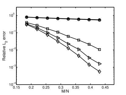
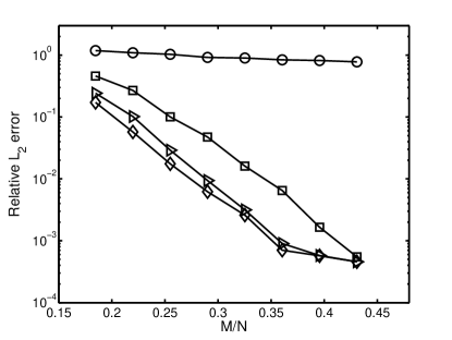
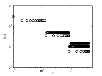
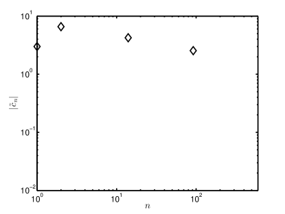
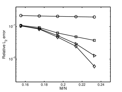
In this test, we set $d=12$ (hence, $N=455$ for $P=3$) and demonstrate the effectiveness of our new method. The integrals for calculating the $L_{2}$ error are computed by a level $4$ sparse grid method, hence they are exact. The relative error of $\ell_{1}$ minimization and OMP are presented in Fig. 1. Clearly, the standard $\ell_{1}$ minimization and OMP are not effective as the relative error is close to $100\%$ even when $M/N>0.4$. Also, the re-weighted $\ell_{1}$ does not help in this case. However, our new iterative rotation demonstrates much better accuracy, especially when $M$ is large. As demonstrated in Fig. 2 the iterative rotation creates a much sparser representation of $u$, hence the efficiency of compressive sensing method is substantially enhanced. We notice that the accuracy increases as more iterations are included. However, the improvement from $6$ iterations to $9$ iterations is less significant as that from $3$ iterations to $6$ iterations, especially for the OMP-based iterative rotation method. In general, the improvement afforded by iterative rotation becomes small after $3$ iterations.

Figure 1: Results for the example function with equally important random variables. (Left) Comparison with the $\ell_{1}$ method. “$\circ$”: $\ell_{1}$, “$\Box$”: rotated $\ell_{1}$ with $3$ iterations, “$\triangleright$”: rotated $\ell_{1}$ with $6$ iterations, “$\diamond$”: rotated $\ell_{1}$ with $9$ iterations, “$*$”: re-weighted $\ell_{1}$. (Right) Comparison with the OMP method. “$\circ$”: OMP, “$\Box$”: rotated OMP with $3$ iterations, “$\triangleright$”: rotated OMP with $6$ iterations, “$\diamond$”: rotated OMP with $9$ iterations. These calculations were performed with dimension $d=12$ and the number of unknowns $N=455$.

Figure 2: Magnitude of the gPC coefficients for the example function with equally important random variables. (Left) Magnitude of $\bm{c}_{n}$. (Right) Magnitude of $\tilde{\bm{c}}_{n}$ of a randomly chosen replicate computed by rotated $\ell_{1}$ with $9$ iterations and $M=180$ ($M/N\approx 0.4$). These calculations were performed with dimension $d=12$ and the number of unknowns $N=455$.

This contrived example demonstrates that our new method is capable of enhancing the sparsity of the Hermite polynomial expansion, even with a very inaccurate $\tilde{\bm{c}}^{(0)}$ in Step 2 of Algorithm 3 when other methods fail.

4.2 Example function with high compressibility

Consider the following function:

$$u(\bm{\xi})=\sum_{|\bm{\alpha}|=0}^{P}c_{\bm{\alpha}}\psi_{\bm{\alpha}}(\bm{\xi})=\sum_{n=1}^{N}c_{n}\psi_{n}(\bm{\xi}),\quad\bm{\xi}=(\xi_{1},\xi_{2},\cdots,\xi_{d}),$$ (4.3)

where, $\psi_{\bm{\alpha}}$ are normalized multivariate Hermite polynomials, $d=12,P=3,N=455$, and the coefficients $c_{n}$ are chose as uniformly distributed random numbers,

$$c_{n}=\zeta/n^{1.5},\quad\zeta\sim\mathcal{U}[-1,1].$$ (4.4)

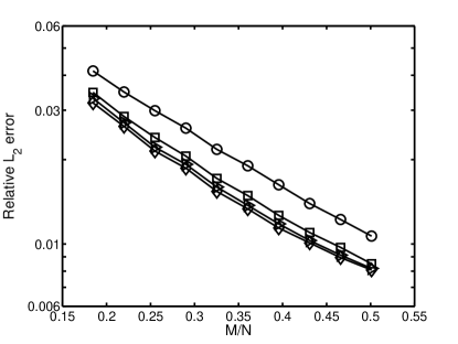
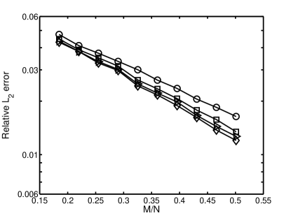
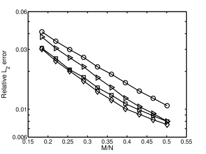
For this example, we generate $N$ samples of $\zeta$: $\zeta^{1},\zeta^{2},\cdots,\zeta^{N}$ then divide them by $n^{1.5},n=1,2,\cdots,N$ to obtain a random “compressible signal” $\bm{c}$. The integrals for the relative error are computed by a level-$4$ sparse grid method and are therefore exact. Figure 3 shows the the relative error with different numbers of iterations ($1$-$3$) for the $\ell_{1}$ minimization and OMP methods. Our new iterative rotation method improves the accuracy of the gPC approximation for both methods. As before, benefit of increased iterations drops sharply near $L=3$. Therefore, in the remainder of this paper we use $L=3$ iterations unless otherwise noted.

Figure 3: Results for the example function with high compressibility. Relative $L_{2}$ error for different numbers of iterations for $\ell_{1}$ minimization (left) and the OMP method (right). “$\circ$”: standard $\ell_{1}$ (left) or standard OMP (right), “$\Box$”: $1$ iteration, “$\triangleright$”: $2$ iterations, “$\diamond$”: $3$ iterations. These calculations were performed with dimension $d=12$ and number of unknowns $N=455$.

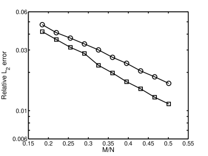
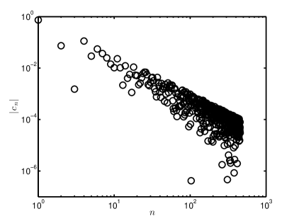
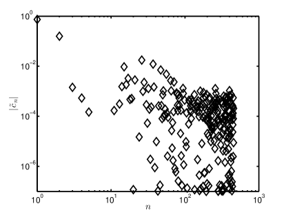
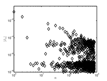
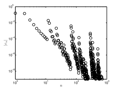
Figure 4 shows results obtained by applying our iterative rotation technique to the re-weighted $\ell_{1}$ approach using $L=3$ iterations. The results for the iterative rotation approach for OMP are also presented in Figure 4. For all methods, introduction of the iterative rotation approach improves the results. A comparison of the sparsity of $\bm{c}$ and $\tilde{\bm{c}}$ is presented in Fig. (5). The main improvement is that the number of coefficients with magnitude larger than $0.01$ is decreased. Also, $|c_{n}|$ cluster around the line $|c_{n}|=1/n^{1.5}$ as we set them in this way, while many $|\tilde{c}_{n}|$ are much below this line especially when $n$ is large.

Figure 4: Results for the example function with high compressibility. (Left) Comparison with $\ell_{1}$ methods. “$\circ$”: standard $\ell_{1}$, “$\triangleright$”: re-weighted $\ell_{1}$, “$\Box$”: rotated $\ell_{1}$, “$\diamond$”: re-weighted and iteratively rotated $\ell_{1}$. (Right) Comparison with OMP methods. “$\circ$”: OMP, “$\Box$”: rotated OMP. These calculations were performed with dimension $d=12$ and number of unknowns $N=455$.

Figure 5: Magnitude of the gPC coefficients for example function with high compressibility. (Left) Magnitude of $\bm{c}_{n}$. (Right) Magnitude of $\tilde{\bm{c}}_{n}$ of a randomly chosen replicate computed by re-weighted and iteratively rotated $\ell_{1}$ with $M=180$ ($M/N\approx 0.4$). These calculations were performed with dimension $d=12$ and the number of unknowns $N=455$.

4.3 Example elliptic differential equation

Next we consider a one-dimensional elliptic differential equation with a random high-order coefficient:

$$-\frac{d}{dx}\left(a(x;\bm{\xi})\frac{du(x;\bm{\xi})}{dx}\right)=1, \quad x\in(0,1)$$ (4.5)

$$u(0)=u(1)=0,$$

where $a(x;\bm{\xi})$ is a log-normal random field based on Karhunen-Loève (KL) expansion:

$$a(x;\bm{\xi})=a_{0}(x)+\exp\left(\sigma\sum_{i=1}^{d}\sqrt{\lambda_{i}}\phi_{i}(x)\xi_{i}\right),$$ (4.6)

where $\{\xi_{i}\}$ are i.i.d. standard Gaussian random variables, $\{\lambda_{i}\}_{i=1}^{d}$, and $\{\phi_{i}(x)\}_{i=1}^{d}$ are the largest eigenvalues and corresponding eigenfunctions of the exponential covariance kernel:

$$C(x,x^{\prime})=\exp\left(\dfrac{|x-x^{\prime}|}{l_{c}}\right).$$ (4.7)

In the KL expansion, $\lambda_{i}$ denotes the eigenvalue of the covariance kernel $C(x,x^{\prime})$ instead of entries of $\Lambda$ in Eq. (3.5). The value of $\lambda_{i}$ and the analytical expressions for $\phi_{i}$ are available in the literature [49]. In this example, we set $a_{0}(x)\equiv 0.1,\sigma=0.5,l_{c}=0.2$ and $d=15$. With this setting, $\sum_{i=1}^{d}\lambda_{i}>0.93\sum_{i=1}^{\infty}\lambda_{i}$. For each input sample $\bm{\xi}^{q}$, $a$ and $u$ only depend on $x$ and the solution of the deterministic elliptic equation can be obtained as [15]:

$$u(x)=u(0)+\int_{0}^{x}\dfrac{a(0)u(0)^{\prime}-y}{a(y)}\mathrm{d}y.$$ (4.8)

By imposing the boundary condition $u(0)=u(1)=0$, we can compute $a(0)u(0)^{\prime}$ as

$$a(0)u(0)^{\prime}=\left(\int_{0}^{1}\dfrac{y}{a(y)}\mathrm{d}y\right)\Big{/}\left(\int_{0}^{1}\dfrac{1}{a(y)}\mathrm{d}y\right).$$ (4.9)

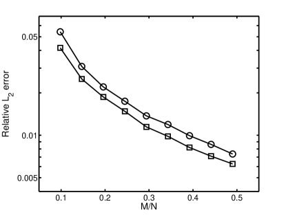
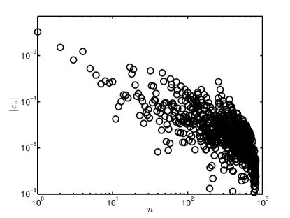
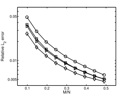
The integrals in Eqs. (4.9) and (4.8) must be obtained by highly accurate numerical integration. For this example, we choose the quantity of interest to be $u(x;\bm{\xi})$ at $x=0.35$. We aim to build a 3rd-order Hermite polynomial expansion which includes $N=816$ basis functions. The relative error is approximated by a level-$6$ sparse grid method. Figure 6 shows that accuracy of the re-weighted $\ell_{1}$ ($3$ iterations) and the iteratively rotated $\ell_{1}$ ($L=3$ iterations) method are very close in this case. Figure 6 shows the results of the iterative rotation process applied to the OMP method. In all cases, the incorporation of iterative rotation improves the performance of the other methods. A comparison of $\bm{c}$ and $\tilde{\bm{c}}$ are presented in Fig. 7, which shows the improvement of the sparsity in the similar manner as in example function with high compressibility in Sec. 4.2.

Figure 6: Results for the example elliptic differential equation. (Left) Comparison with $\ell_{1}$ methods. “$\circ$”: standard $\ell_{1}$, “$\triangleright$”: re-weighted $\ell_{1}$, “$\Box$”: rotated $\ell_{1}$, “$\diamond$”: re-weighted and iteratively rotated $\ell_{1}$. (Right) Comparison with OMP methods. “$\circ$”: standard OMP, “$\Box$”: rotated OMP. These calculations were performed with dimension $d=15$ and the number of unknowns $N=816$.

Figure 7: Magnitude of the gPC coefficients for example elliptic differential equation. (Left) Magnitude of $\bm{c}_{n}$. (Right) Magnitude of $\tilde{\bm{c}}_{n}$ of a randomly chosen replicate computed by re-weighted and iteratively rotated $\ell_{1}$ with $M=240$ ($M/N\approx 0.3$). These calculations were performed with dimension $d=15$ and the number of unknowns $N=816$.

4.4 Example Korteweg-de Vries equation

As an example application of our new method to a more complicated and nonlinear differential equation, we consider the Korteweg-de Vries (KdV) equation with time-dependent additive noise [50]:

$$u_{t}(x,t;\bm{\xi})-6u(x,t;\bm{\xi})u_{x}(x,t;\bm{\xi})+u_{xxx}(x,t;\bm{\xi})=f(t;\bm{\xi}),\quad x\in(-\infty,\infty),$$ (4.10)

$$u(x,0;\bm{\xi})=-2\operatorname{sech}^{2}(x).$$

Defining

$$W(t;\bm{\xi})=\int_{0}^{t}f(y;\bm{\xi})\mathrm{d}y,$$ (4.11)

the analytical solution of Eq. (4.10) is

$$u(x,t;\bm{\xi})=W(t;\bm{\xi})-2\operatorname{sech}^{2}\left(x-4t+6\int_{0}^{t}W(z;\bm{\xi})\mathrm{d}z\right).$$ (4.12)

We model $f(t;\bm{\xi})$ as a Gaussian random field represented by the following KL expansion:

$$f(t;\bm{\xi})=\sigma\sum_{i=1}^{d}\sqrt{\lambda_{i}}\phi_{i}(t)\xi_{i},$$ (4.13)

where $\sigma$ is a constant and $\{\lambda_{i},\phi_{i}(t)\}_{i=1}^{d}$ are eigenpairs of the exponential covariance kernel as in Eqs. (4.6) and (4.7), respectively. In this problem, we set $l_{c}=0.25$ and $d=10$ ($\sum_{i=1}^{d}\lambda_{i}>0.96\sum_{i=1}^{\infty}\lambda_{i}$). In this case, the exact one-soliton solution is

$$u(x,t;\bm{\xi})=\sigma\sum_{i=1}^{d}\sqrt{\lambda_{i}}\xi_{i}\int_{0}^{t}\phi_{i}(y)\mathrm{d}y-2\operatorname{sech}^{2}\left(x-4t+6\sigma\sum_{i=1}^{d}\sqrt{\lambda_{i}}\xi_{i}\int_{0}^{t}\int_{0}^{z}\phi_{i}(y)\mathrm{d}y\mathrm{d}z\right).$$ (4.14)

Since an analytical expression for $\phi_{i}$ is available, we can compute the integrals in Eq. (4.14) with high accuracy. Denoting

$$A_{i}=\sqrt{\lambda_{i}}\int_{0}^{t}\phi_{i}(y)\mathrm{d}y,\quad B_{i}=\sqrt{\lambda_{i}}\int_{0}^{t}\int_{0}^{z}\phi_{i}(y)\mathrm{d}y\mathrm{d}z,\quad i=1,2,\cdots,d,$$ (4.15)

the analytical solution is

$$u(x,t;\bm{\xi})\big{|}_{x=6,t=1}=\sigma\sum_{i=1}^{d}A_{i}\xi_{i}-2\operatorname{sech}^{2}\left(2+6\sigma\sum_{i=1}^{d}B_{i}\xi_{i}\right).$$ (4.16)

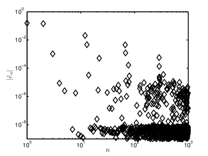
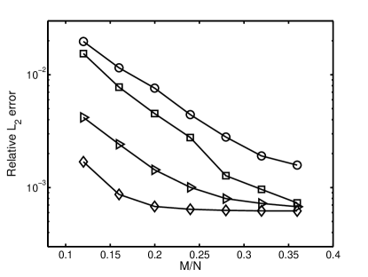
The quantity of interest is chosen to be $u(x,t;\bm{\xi})$ at $x=6,t=1$ with $\sigma=0.1$, $P=4$, and the number of gPC basis functions $N=1001$. For this example, the combined iterative rotation and re-weighted $\ell_{1}$ method outperforms all other approaches. However, unlike previous examples the non-rotated re-weighted $\ell_{1}$ method works better than our iteratively rotated unweighted method. This difference likely arises because $\bm{c}$ is sparser in this case than in others, which makes re-weighted $\ell_{1}$ method more efficient. The pattern of sparsity in this case is different than previous examples, hence the efficiency of identifying a good rotation matrix $\mathsfsl{A}$ is different. A comparison of $\bm{c}$ and $\tilde{\bm{c}}$ are presented in Fig. 9, which shows the improvement of the sparsity by the iterative rotation method.

Figure 8: Results for the example KdV equation. (Left) Comparison to $\ell_{1}$ methods. “$\circ$”: standard $\ell_{1}$, “$\triangleright$”: re-weighted $\ell_{1}$, “$\Box$”: rotated $\ell_{1}$, “$\diamond$”: re-weighted and iteratively rotated $\ell_{1}$. (Right) Comparison to the OMP method. $\circ$”: standard OMP, “$\Box$”: rotated OMP. The dimension is $d=10$ and the number of unknowns is $N=1001$.

Figure 9: Magnitude of the gPC coefficients for example KdV equation. (Left) Magnitude of $\bm{c}_{n}$. (Right) Magnitude of $\tilde{\bm{c}}_{n}$ of a randomly chosen replicate computed by re-weighted and iteratively rotated $\ell_{1}$ with $M=120$ ($M/N\approx 0.12$). These calculations were performed with dimension $d=10$ and the number of unknowns $N=1001$.

4.5 Example high-dimensional function

The previous examples demonstrate the capability of our new method to solve moderately high-dimensional problems. In the last example, we illustrate its potential for dealing with higher-dimensional problems. Specially, we select a function similar to the first example (Sec. 4.1) but with much higher dimensionality:

$$u(\bm{\xi})=\sum_{i=1}^{d}\xi_{i}+0.25\left(\sum_{i=1}^{d}\xi_{i}/\sqrt{i}\right)^{2},\quad d=100.$$ (4.17)

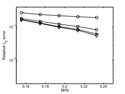
The total number of basis functions for this example is $N=5151$. The relative error is computed with a level-$3$ sparse grid method, hence the numerical integrals are exact. The results are presented in Fig. 10. As before, our iterative rotation approach out-performs the existing $\ell_{1}$ and OMP methods. A comparison of $\bm{c}$ and $\tilde{\bm{c}}$ is presented in Fig. 11 and it shows the enhancement of the sparsity by the iterative rotation method.

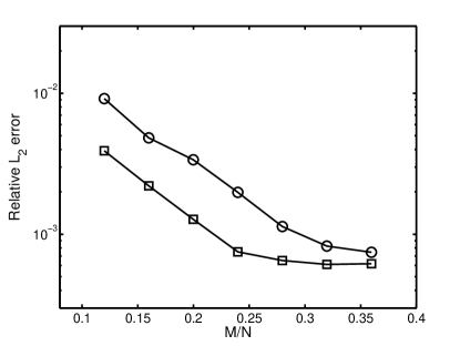
For general high-dimensional problems, simply truncating the gPC expansion up to a certain order is not efficient because the number of basis function will be very large. For example, in this test, $P=2$ requires $5151$ basis functions. Under such conditions even a small $M/N=0.2$ needs $1030$ samples, which can be difficult in practical problems when the computational model is very costly. Hence, a good approach for high-dimensional problems is to integrate our iterative rotation method with an adaptive method to reduce $N$; e.g., adaptive basis selection [22] or an ANOVA method [47]).

Figure 10: Results for the example high-dimensional function. (Left) Comparison with $\ell_{1}$ methods. “$\circ$”: standard $\ell_{1}$, “$\Box$”: rotated $\ell_{1}$ with $1$ iterations, “$\triangleright$”: rotated $\ell_{1}$ with $2$ iterations; “$\diamond$”: rotated $\ell_{1}$ with $3$ iterations. (Right) Comparison with OMP methods. “$\Box$”: rotated OMP with $1$ iterations, “$\triangleright$”: rotated OMP with $2$ iterations; “$\diamond$”: rotated OMP with $3$ iterations. These calculations were performed with $d=100$ and the number of unknowns $N=5151$.

Figure 11: Magnitude of the gPC coefficients for example high-dimensional function. (Left) Magnitude of $\bm{c}_{n}$. (Right) Magnitude of $\tilde{\bm{c}}_{n}$ of a randomly chosen replicate computed by $3$ iterated OMP method with $M=1200$ ($M/N\approx 0.23$). These calculations were performed with dimension $d=100$ and the number of unknowns $N=5151$.

4.6 Accuracy of computing the expansion coefficients $\bm{c}$

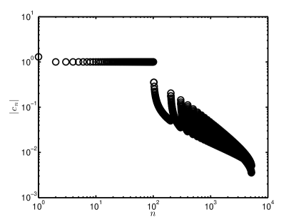
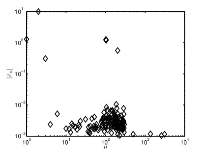
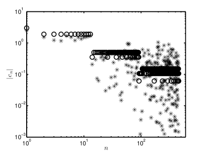
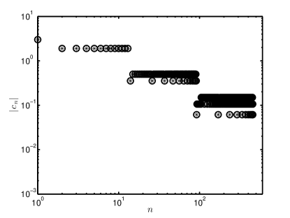
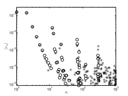
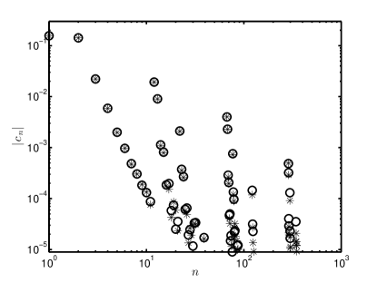
In many applications, gPC expansions are also used to study the sensitivity of the quantity of interest to the input random variables $\bm{\xi}$. In order to perform this analysis, we need to transform the $u_{g}(\bm{\eta})=\sum_{n=1}^{N}\tilde{c}_{n}\psi_{n}(\bm{\eta})$ back to the original variables $u_{g}(\bm{\xi})=\sum_{n=1}^{N}c_{n}\psi_{n}(\bm{\xi})$. This transformation can be accomplished through inversion of $\mathsfsl{A}$ in $\bm{\eta}=\mathsfsl{A}\bm{\xi}$. In Figures 12 and 13, we present the coefficients of $u_{g}(\bm{\xi})$ in examples 4.1 and 4.4, respectively. In both figures we randomly choose one test from the $100$ replicates. In Figure 12, we select a result with $M=180$ ($M/N\approx 0.4$). Using the standard $\ell_{1}$ method (left) gives very inaccurate results for $\bm{c}$. However, Figure 12 (right) shows that the iterative rotation method with $L=9$ iterations gives much more accurate results for $\bm{c}$. We observe the same behavior in Figure 13, where we chose a test with $M=120$ ($M/N\approx 0.12$) for the example KdV equation (Sec. 4.4). In order to make this figure legible, we only present those $c_{i}$ with absolute value larger than $10^{-5}$. This example demonstrates that coefficients $c_{n}$ with magnitude larger than $10^{-3}$ are computed accurately by the combined iterative rotation and re-weighted $\ell_{1}$ method while the standard $\ell_{1}$ obtained significantly less accurate $c_{n}$. This difference is more distinct for $|c_{n}|\in[10^{-4},10^{-3}]$; in this range our new method compute $c_{n}$ much more accurate than the standard $\ell_{1}$ method. In the lower right corner of the left plot, the standard $\ell_{1}$ method yields many $c_{n}$ which should not appear in that area. As a comparison, we do not see such $c_{n}$ calculated with the new method.

Figure 12: Comparison of gPC coefficients for the example function with equally important random variables (Sec. 4.1). (Left) Coefficients calculated by the standard $\ell_{1}$ method. “$\circ$”: exact $|c_{i}|$; “$*$”: $|c_{i}|$ by standard $\ell_{1}$ method. (Right) Coefficients calculated by our new iteratively rotated $\ell_{1}$ method with $L=9$ iterations.

Figure 13: Comparison of gPC coefficients for solutions of the KdV equation (Sec. 4.4). (Left) Coefficients calculated with the standard $\ell_{1}$ method. “$\circ$”: “exact” $|c_{i}|$; “$*$”: $|c_{i}|$ by standard $\ell_{1}$ method. (Right) Coefficients calculated by our new iteratively rotated re-weighted $\ell_{1}$ method (right). Only $|c_{i}|>10^{-5}$ are presented.

5 Conclusions

In this paper, we extend our previous work [17] and have introduced a compressive sensing-based gPC method to increase the sparsity and accuracy of Hermite polynomial expansion with iterative rotations. Similar to the active subspace method [28, 17], the rotation is decided by seeking the directions of maximum variation for the quantity of interest. Our current numerical examples are intended to demonstrate the ability of the method to increase the sparsity and accuracy of the gPC expansion; therefore, the quantity of interest only relies on the random variables. It is also possible to include the physical variables in the basis functions, i.e., $u(\bm{x};\bm{\xi})=\sum_{n}c_{n}\psi_{n}(\bm{x};\bm{\xi})$ (e.g, [16]), our future work will explore how this new method may help to increase the sparsity in such cases.

We have demonstrated the method for $\ell_{1}$ minimization and OMP methods but it can also be integrated with other compressive sensing methods. In particular, future work will investigate the integration of our new methods with advanced sampling strategies (e.g., [20]), adaptive basis selection method (e.g., [22]), Bayesian compressive sensing method (e.g.,[16]), etc. These advanced strategies are particularly important for high-dimensional problems.

With this method, we will also be able to construct an accurate surrogate model of the quantity of interest with limited data. Surrogate models are specifically useful for the problems where the experiments or simulations are very costly. This surrogate model can be used to study the sensitivity of the parameters and is very useful in inverse problems based on Bayesian framework. Our new method requires fewer output data to construct such surrogate models, which can be a great savings of experimental or computational resources.

Finally, we highlight three additional areas of future work for improving the new method. First, it is currently only suitable for Hermite polynomial expansions. Second, the new method requires a formal numerical analysis to assess convergence behavior and determine specific terminating criteria. Finally, there are likely more optimal iterative rotation strategies that can be applied to Hermite polynomial or other expansions. One possible direction of work is to design a suitable objective function and consider this problem from an optimization point of view. All of these questions will be addressed in our future work.

Appendix

Here we provide the details of computing the elements $(K_{ij})_{kl}$ in Eq. (3.6). Notice that for univariate normalized Hermite polynomials,

$$\psi_{n}(\xi)^{\prime}=\sqrt{n}\psi_{n-1}(\xi),\quad n\in\mathbb{N}\cup\{0\},$$ (A-1)

where we set $\psi_{-1}(\xi)=0$ for simplicity. Therefore, we have

$$\mathbb{E}\left\{{\psi_{i}(\xi)^{\prime}\psi_{j}(\xi)}\right\}=\int_{\mathbb{R}}\psi_{i}(\xi)^{\prime}\psi_{j}(\xi)\rho(\xi)\mathrm{d}\xi=\sqrt{i}\delta_{i-1j},$$ (A-2)

where $\rho(\xi)$ is the PDF of a standard Gaussian random variable. For a multi-index $\bm{\alpha}=(\alpha_{1},\alpha_{2},\cdots,\alpha_{d}),\alpha_{i}\in\mathbb{N}\cup\{0\}$, and basis function $\psi_{\bm{\alpha}}(\bm{\xi})=\psi_{\alpha_{1}}(\xi_{1})\psi_{\alpha_{2}}(\xi_{2})\cdots\psi_{\alpha_{d}}(\xi_{d})$,

$$\dfrac{\partial}{\partial\xi_{i}}\psi_{\bm{\alpha}}(\bm{\xi})=\psi_{\alpha_{i}}(\xi_{i})^{\prime}\prod_{\begin{subarray}{c}m=1\\ m\neq i\end{subarray}}^{d}\psi_{\alpha_{m}}(\xi_{m}).$$ (A-3)

Hence, given two different multi-indices $\bm{\alpha}_{k}=((\alpha_{k})_{{}_{1}},(\alpha_{k})_{{}_{2}},\cdots,(\alpha_{k})_{{}_{d}})$ and $\bm{\alpha}_{l}=((\alpha_{l})_{{}_{1}},(\alpha_{l})_{{}_{2}},\cdots,(\alpha_{l})_{{}_{d}})$, the corresponding entry of matrix $\mathsfsl{K}_{ij}$ is

$$(K_{ij})_{kl} =\mathbb{E}\left\{{\dfrac{\partial\psi_{\bm{\alpha}_{k}}(\bm{\xi})}{\partial\xi_{i}}\cdot\dfrac{\partial\psi_{\bm{\alpha}_{l}}(\bm{\xi})}{\partial\xi_{j}}}\right\}$$ (A-4)

$$=\mathbb{E}\left\{{\left(\psi_{(\alpha_{k})_{{}_{i}}}(\xi_{i})^{\prime}\prod_{\begin{subarray}{c}m=1\\ m\neq i\end{subarray}}^{d}\psi_{(\alpha_{k})_{{}_{m}}}(\xi_{m})\right)\cdot\left(\psi_{(\alpha_{l})_{{}_{j}}}(\xi_{j})^{\prime}\prod_{\begin{subarray}{c}m=1\\ m\neq j\end{subarray}}^{d}\psi_{(\alpha_{l})_{{}_{m}}}(\xi_{m})\right)}\right\}$$

$$=\sqrt{(\alpha_{k})_{{}_{i}}(\alpha_{l})_{{}_{j}}}\delta_{(\alpha_{k})_{{}_{i}}-1(\alpha_{l})_{{}_{i}}}\delta_{(\alpha_{k})_{{}_{j}}(\alpha_{l})_{{}_{j}}-1}\cdot\prod_{\begin{subarray}{c}m=1\\ m\neq i,m\neq j\end{subarray}}\delta_{(\alpha_{k})_{{}_{m}}(\alpha_{l})_{{}_{m}}}.$$

References

• [1] R. G. Ghanem, P. D. Spanos, Stochastic finite elements: a spectral approach, Springer-Verlag, New York, 1991.
• [2] D. Xiu, G. E. Karniadakis, The Wiener-Askey polynomial chaos for stochastic differential equations, SIAM J. Sci. Comput. 24 (2) (2002) 619–644.
• [3] R. H. Cameron, W. T. Martin, The orthogonal development of non-linear functionals in series of fourier-hermite functionals, Annals of Mathematics (1947) 385–392.
• [4] H. Ogura, Orthogonal functionals of the poisson process, Information Theory, IEEE Transactions on 18 (4) (1972) 473–481.
• [5] M. A. Tatang, W. Pan, R. G. Prinn, G. J. McRae, An efficient method for parametric uncertainty analysis of numerical geophysical models, J. Geophys. Res-Atmos. (1984–2012) 102 (D18) (1997) 21925–21932.
• [6] D. Xiu, J. S. Hesthaven, High-order collocation methods for differential equations with random inputs, SIAM J. Sci. Comput. 27 (3) (2005) 1118–1139.
• [7] J. Foo, X. Wan, G. E. Karniadakis, The multi-element probabilistic collocation method (ME-PCM): error analysis and applications, J. Comput. Phys. 227 (22) (2008) 9572–9595.
• [8] I. Babuška, F. Nobile, R. Tempone, A stochastic collocation method for elliptic partial differential equations with random input data, SIAM Rev. 52 (2) (2010) 317–355.
• [9] E. J. Candès, J. K. Romberg, T. Tao, Stable signal recovery from incomplete and inaccurate measurements, Comm. Pure Applied Math. 59 (8) (2006) 1207–1223.
• [10] D. L. Donoho, M. Elad, V. N. Temlyakov, Stable recovery of sparse overcomplete representations in the presence of noise, IEEE Trans. Inform. Theory 52 (1) (2006) 6–18.
• [11] E. J. Candès, The restricted isometry property and its implications for compressed sensing, C. R. Math. Acad. Sci. Paris 346 (9-10) (2008) 589–592.
• [12] A. M. Bruckstein, D. L. Donoho, M. Elad, From sparse solutions of systems of equations to sparse modeling of signals and images, SIAM Rev. 51 (1) (2009) 34–81.
• [13] A. Doostan, H. Owhadi, A non-adapted sparse approximation of PDEs with stochastic inputs, J. Comput. Phys. 230 (8) (2011) 3015–3034.
• [14] L. Yan, L. Guo, D. Xiu, Stochastic collocation algorithms using l1subscript𝑙1l_{1}-minimization, Int. J. Uncertainty Quantification 2 (3) (2012) 279–293.
• [15] X. Yang, G. E. Karniadakis, Reweighted 1subscript1\ell_{1} minimization method for stochastic elliptic differential equations, J. Comput. Phys. 248 (1) (2013) 87–108.
• [16] G. Karagiannis, B. A. Konomi, G. Lin, A bayesian mixed shrinkage prior procedure for spatial–stochastic basis selection and evaluation of gpc expansions: Applications to elliptic spdes, J. Comput. Phys. 284 (2015) 528–546.
• [17] H. Lei, X. Yang, B. Zheng, G. Lin, N. A. Baker, Quantifying the influence of conformational uncertainty in biomolecular solvation, arXiv preprint arXiv:1408.5629.
• [18] J. Peng, J. Hampton, A. Doostan, A weighted 1subscript1\ell_{1}-minimization approach for sparse polynomial chaos expansions, J. Comput. Phys. 267 (0) (2014) 92 – 111.
• [19] Z. Xu, T. Zhou, On sparse interpolation and the design of deterministic interpolation points, SIAM J. Sci. Comput. 36 (4) (2014) A1752–A1769.
• [20] J. Hampton, A. Doostan, Compressive sampling of polynomial chaos expansions: Convergence analysis and sampling strategies, J. Comput. Phys. 280 (0) (2015) 363 – 386.
• [21] G. Tang, G. Iaccarino, Subsampled gauss quadrature nodes for estimating polynomial chaos expansions, SIAM J. Uncertainty Quantification 2 (1) (2014) 423–443.
• [22] J. D. Jakeman, M. S. Eldred, K. Sargsyan, Enhancing 1subscript1\ell_{1}-minimization estimates of polynomial chaos expansions using basis selection, J. Comput. Phys. 289 (2015) 18–34.
• [23] K. Sargsyan, C. Safta, H. N. Najm, B. J. Debusschere, D. Ricciuto, P. Thornton, Dimensionality reduction for complex models via bayesian compressive sensing, Int. J. Uncertainty Quantification 4 (1).
• [24] J. Peng, J. Hampton, A. Doostan, On polynomial chaos expansion via gradient-enhanced 1subscript1\ell_{1}-minimization, arXiv preprint arXiv:1506.00343.
• [25] E. J. Candès, M. B. Wakin, S. P. Boyd, Enhancing sparsity by reweighted l1subscript𝑙1l_{1} minimization, J. Fourier Anal. Appl. 14 (5-6) (2008) 877–905.
• [26] H. Rauhut, R. Ward, Interpolation via weighted ℓ1 minimization, Applied and Computational Harmonic Analysis.
• [27] H. Rauhut, R. Ward, Sparse legendre expansions via l1subscript𝑙1l_{1}-minimization, J. Approx. Theory 164 (5) (2012) 517–533.
• [28] P. G. Constantine, E. Dow, Q. Wang, Active subspace methods in theory and practice: Applications to kriging surfaces, SIAM J. Sci. Comput. 36 (4) (2014) A1500–A1524.
• [29] S. S. Chen, D. L. Donoho, M. A. Saunders, Atomic decomposition by basis pursuit, SIAM J. Sci. Comput. 20 (1) (1998) 33–61.
• [30] S. Boyd, L. Vandenberghe, Convex optimization, Cambridge university press, 2004.
• [31] D. L. Donoho, Compressed sensing, IEEE Trans. Inf. Theory 52 (4) (2006) 1289–1306.
• [32] E. J. Candès, T. Tao, Decoding by linear programming, IEEE Trans. Inform. Theory 51 (12) (2005) 4203–4215.
• [33] D. Needell, Noisy signal recovery via iterative reweighted l1subscript𝑙1l_{1} minimization, in: Proc. Asilomar Conf. on Signal Systems and Computers, Pacific Grove, CA, 2009.
• [34] J. A. Tropp, Greed is good: Algorithmic results for sparse approximation, IEEE Trans. Inform. Theory 50 (10) (2004) 2231–2242.
• [35] J. A. Tropp, A. C. Gilbert, Signal recovery from random measurements via orthogonal matching pursuit, IEEE Trans. Inform. Theory 53 (12) (2007) 4655–4666.
• [36] J. W. Hardin, J. Hilbe, Generalized linear models and extensions, Stata Press, 2007.
• [37] Y. Xia, A constructive approach to the estimation of dimension reduction directions, Ann. Stat. (2007) 2654–2690.
• [38] O. Roderick, M. Anitescu, P. Fischer, Polynomial regression approaches using derivative information for uncertainty quantification, Nucl. Sci. Eng. 164 (2) (2010) 122–139.
• [39] Y. Li, M. Anitescu, O. Roderick, F. Hickernell, Orthogonal bases for polynomial regression with derivative information in uncertainty quantification, Int. J. Uncertainty Quantification 1 (4).
• [40] B. Lockwood, D. Mavriplis, Gradient-based methods for uncertainty quantification in hypersonic flows, Computers & Fluids 85 (2013) 27–38.
• [41] S. Smolyak, Quadrature and interpolation formulas for tensor products of certain classes of functions, Sov. Math. Dokl. 4 (1963) 240–243.
• [42] E. van den Berg, M. P. Friedlander, Probing the pareto frontier for basis pursuit solutions, SIAM Journal on Scientific Computing 31 (2) (2008) 890–912.
• [43] E. van den Berg, M. P. Friedlander, SPGL1: A solver for large-scale sparse reconstruction, http://www.cs.ubc.ca/labs/scl/spgl1 (June 2007).
• [44] D. Donoho, I. Drori, V. Stodden, Y.Tsaig, Sparselab: Seeking sparse solutions to linear systems of equations, http://www-stat.stanford.edu/~sparselab/.
• [45] X. Ma, N. Zabaras, An adaptive hierarchical sparse grid collocation algorithm for the solution of stochastic differential equations, J. Comput. Phys. 228 (8) (2009) 3084–3113.
• [46] X. Ma, N. Zabaras, An adaptive high-dimensional stochastic model representation technique for the solution of stochastic partial differential equations, J. Comput. Phys. 229 (10) (2010) 3884–3915.
• [47] X. Yang, M. Choi, G. Lin, G. E. Karniadakis, Adaptive ANOVA decomposition of stochastic incompressible and compressible flows, J. Comput. Phys. 231 (4) (2012) 1587–1614.
• [48] Z. Zhang, X. Yang, G. Marucci, P. Maffezzoni, I. A. Elfadel, G. Karniadakis, L. Daniel, Stochastic testing simulator for integrated circuits and MEMS: Hierarchical and sparse techniques, in: Custom Integrated Circuits Conference (CICC), 2014 IEEE Proceedings of the, 2014, pp. 1–8.
• [49] M. Jardak, C.-H. Su, G. E. Karniadakis, Spectral polynomial chaos solutions of the stochastic advection equation, J. Sci. Comput. 17 (1-4) (2002) 319–338.
• [50] G. Lin, L. Grinberg, G. E. Karniadakis, Numerical studies of the stochastic korteweg-de vries equation, J. Comput. Phys. 213 (2) (2006) 676–703.