PARSEC evolutionary tracks of massive stars up to 350 $M_{\odot}$ at metallicities 0.0001$\mn@boldsymbol{\leq Z\leq}$0.04

Abstract

We complement the PARSEC data base of stellar evolutionary tracks with new models of massive stars, from the pre-main sequence phase to the central Carbon ignition. We consider a broad range of metallicities, 0.0001$\leq Z\leq$0.04 and initial masses up to $M_{\rm ini}$=$350\,\mbox{$M_{\odot}$}$. The main difference with respect to our previous models of massive stars is the adoption of a recent formalism accounting for the mass-loss enhancement when the ratio of the stellar to the Eddington luminosity, $\Gamma_{e}$, approaches unity. With this new formalism, the models are able to reproduce the Humphreys-Davidson limit observed in the Galactic and Large Magellanic Cloud colour-magnitude diagrams, without an ad hoc mass-loss enhancement. We also follow the predictions of recent wind models indicating that the metallicity dependence of the mass-loss rates becomes shallower when $\Gamma_{e}$ approaches unity. We thus find that the more massive stars may suffer from substantial mass-loss even at low metallicity. We also predict that the Humphreys-Davidson limit should become brighter at decreasing metallicity. We supplement the evolutionary tracks with new tables of theoretical bolometric corrections, useful to compare tracks and isochrones with the observations. For this purpose, we homogenize existing stellar atmosphere libraries of hot and cool stars (PoWR, ATLAS9 and Phoenix) and we add, where needed, new atmosphere models computed with WM-basic. The mass, age and metallicity grids are fully adequate to perform detailed investigations of the properties of very young stellar systems, both in local and distant galaxies. The new tracks supersede the previous old Padova models of massive stars.

1 Introduction

Massive stars play an important role in the evolution of galaxies. They are the most important stellar sources of ionizing and dissociation photons (Schaerer et al., 2011; Kimm & Cen, 2014; Dale, Ercolano & Bonnell, 2012; Cai et al., 2014; Hollenbach & Tielens, 1999; Yu, Wang & Li, 2015). They inject a significant amount of kinetic energy through powerful stellar winds (Mackey et al., 2014). They are among the main drivers of metal and dust enrichment in galaxies when they explode as core collapsed supernovae (SNe) (Sarangi & Cherchneff, 2015; Schneider, Ferrara & Salvaterra, 2004). They are thus very important sources of feedback to the ambient ISM (Dale, Ercolano & Bonnell, 2013). Last but not least, most of our information on the ongoing star formation rates across the Universe heavily relies on our detailed knowledge of their properties (Bruzual & Charlot, 2003; Kennicutt, 1998).

Because of their relevance for so many fields of astrophysics, massive stars have been the subject of many observational and theoretical investigations that are impossible to list here. Understanding their evolution is challenged by the complexity of several physical phenomena, as recently reviewed, for example, by Martins & Palacios (2013) who compare STERN (Brott et al., 2011), Geneva (Ekström et al., 2012), FRANEC (Chieffi & Limongi, 2013), Padova (Bertelli et al., 2009), MESA (Paxton et al., 2011) and STAREVOL (Decressin et al., 2009) evolutionary tracks of massive stars. Martins & Palacios (2013) find that, apart from the inclusion of rotation, the main differences among the models computed by different authors can be attributed to the different treatments of convection and mass-loss, with the former process being more important in the domain of the less massive stars. It is worth noting that the Padova tracks (Bertelli et al., 2009) analyzed by Martins & Palacios (2013) are still those presented in  Fagotto et al. (1994) and Bressan et al. (1993). Since then, there have been many advances both in the basic input physics (opacities, equation of state, nuclear reactions) and in the mass-loss theory (and observations), and these called for a substantial revision of the Padova code. But, while low and intermediate mass stars were systematically updated, with the last version being PARSEC (PAdova T​ Rieste  Stellar  Evolution  Code) models (Bressan et al., 2012, and refs. therein), massive stars have not been updated since then.

In this paper we present the new evolutionary tracks of massive stars computed with PARSEC. Besides the basic input physics, which is described elsewhere (Bressan et al., 2012, and refs. therein), the main novelties concern the recipes adopted for the mass-loss rates and the spectral energy distributions used to convert the tracks from the theoretical to the observational plane. Concerning mass-loss, there have been many efforts over the past years to determine/predict the mass-loss rates of massive stars across different spectral types and metallicities. It is now widely accepted that hot massive blue supergiants (BSG) and Wolf-Rayet (WR) stars lose a prominent amount of their mass through line-driven stellar winds and that the mass-loss rates show a simple scaling law with the metallicity  (Castor, Abbott & Klein, 1975; Kudritzki & Puls, 2000; Nugis & Lamers, 2000; Vink, de Koter & Lamers, 2000, 2001; Muijres et al., 2012b; Crowther, 2007; Smith, 2014). In Luminous Blue Variable (LBV) stars, there is evidence that an important mode of mass-loss is through eruptive mass-loss, that may contribute as much as or even more than the steady stellar wind (Smith, 2009). In this phase the mass-loss rate may easily reach a few of $10^{-4}\mbox{$M_{\odot}$}\,yr^{-1}$ (Lamers, 1989). This eruptive mechanism is still unknown but the observed rates could be explained by a super-Eddington wind (Smith & Owocki, 2006), or by non-disruptive hydrodynamic explosions (Barsukova et al., 2014). Interestingly, LBV stars are found near the so-called Humphreys-Davidson limit (Humphreys & Davidson, 1979) which delimits the forbidden region above which only very few stars are observed in the Hertzsprung-Russell (HR) diagram of the Galactic massive stars. In this respect, a remarkable result of recent investigations is that the mass-loss rates could be enhanced by a significant factor when the stars approach the Eddington luminosity (Gräfener & Hamann, 2008; Vink et al., 2011), which is known to happen near the Humphreys & Davidson (1979) limit. For the later spectral types there are larger uncertainties both on the mechanisms and on the strength of the mass-loss rates. In red supergiants (RSG) one customarily adopts the observational parametrization by de Jager, Nieuwenhuijzen & van der Hucht (1988), but the mass-loss rates in this phase are known to be uncertain by a large factor (Salasnich, Bressan & Chiosi, 1999; Meynet et al., 2015). As in less massive Asymptotic Giant Branch (AGB) stars, dust formation on the circumstellar envelopes could be one of the possible mechanisms responsible for this enhancement (van Loon et al., 2005).

Concerning the atmosphere models used to predict the stellar magnitudes and colours, they are equally important for the interpretation of observed properties of massive stars. For stars with negligible mass-loss, a comprehensive stellar atmosphere library usually adopted is ATLAS9 (Castelli & Kurucz, 2004), consisting of plane parallel models in local thermodynamic equilibrium. This library is particularly suitable for $\sim$ A, F and G type stars. For cool giants, where the plane parallel and non-LTE (non-local thermodynamic equilibrium) approximations must be relaxed, comprehensive stellar atmosphere libraries are provided by Phoenix (Allard et al., 2012, and references therein) and MARCS (Gustafsson et al., 2008) projects. For hot stars with high mass-loss rates a number of atmosphere models have been released in the recent years like the WM-basic models (Pauldrach, Puls & Kudritzki, 1986), the CMFGEN models (Hillier & Miller, 1998) and the Potsdam Wolf-Rayet (PoWR) models (Gräfener, Koesterke & Hamann, 2002; Hamann & Gräfener, 2003, 2004; Sander, Hamann & Todt, 2012; Hamann, Gräfener & Liermann, 2006; Hainich et al., 2014).

The paper is organized as following. In section 2, we describe our stellar evolution models for massive stars, with particular care to the description of the recipes adopted for the mass-loss rates. In this section we also compare the new models with our previous models and with one set among the most recent models found in literature, FRANEC (Chieffi & Limongi, 2013). In Section 3 we describe in detail the adopted atmosphere models and the procedure used to obtain as much as possible homogeneous sets of bolometric correction tables. Finally, in section 4, we discuss the resulting colour-magnitude diagrams predicted from the new evolutionary tracks and isochrones.

Our evolutionary tracks can be downloaded from http://people.sissa.it/~sbressan/parsec.html, and the isochrones can be downloaded from http://stev.oapd.inaf.it/cgi-bin/cmd.

2 Stellar evolutionary tracks

We compute new tracks of massive stars with the PARSEC code for a wide range of initial metallicities and for initial masses from $M_{\rm ini}$=14 M_⊙ to $M_{\rm ini}$=350 M_⊙. The evolution begins from the pre-main sequence phase and ends at central Carbon ignition. The new evolutionary tracks complement the already existing models of intermediate and low mass stars.

2.1 Basic input physics

The input physics used in PARSEC is already thoroughly described in Bressan et al. (2012), Bressan et al. (2013) and Chen et al. (2014). Below we briefly summarize the main points with particular attention to those more relevant to the massive stars. The equation of state (EOS) is computed with the FreeEOS code of A.W. Irwin. Radiative opacities are from the OPAL project (Iglesias & Rogers, 1996) and, in the low-temperature regime, from the ÆSOPUS project (Marigo & Aringer, 2009). Conductive opacities are included following Itoh et al. (2008). The nuclear reaction rates (p-p chains, CNO tri-cycle, Ne–Na and Mg–Al chains and the most important $\alpha$-capture reactions including the $\alpha$-n reactions) and the corresponding $Q$-values are taken from the recommended rates in the JINA reaclib data base (Cyburt et al., 2010). Electron screening factors for all reactions are from Dewitt, Graboske & Cooper (1973) and Graboske et al. (1973). Finally, electron neutrinos energy losses are computed following Munakata, Kohyama & Itoh (1985), Itoh & Kohyama (1983) and Haft, Raffelt & Weiss (1994).

The metal abundances, 0.0001$\leq$Z$\leq$0.04, follow the partition of Grevesse & Sauval (1998) (GS98) with the recent revision by Caffau et al. (2011). With this revision, the current observed solar metallicity is $Z_{\odot}=0.01524$. The initial Helium content at varying metallicity is determined by $Y=Y_{\rm p}+1.78\times~{}Z$, with $Y_{\rm p}=0.2485$ taken from Komatsu et al. (2011).

2.2 Convection, overshooting and mixing

The mixing length parameter (Böhm-Vitense, 1958), derived from the solar model, is $\alpha_{\rm MLT}=1.74$. We adopt the Schwarzschild criterion (Schwarzschild, 1958) to test the stability of radiative zones against convection. In the presence of a gradient of chemical composition, an alternative criterion is that of Ledoux (Ledoux, 1947). This condition may happen during the evolution of massive stars when the convective core grows in mass or when an intermediate radiative region of varying chemical composition becomes unstable to the convection. In this paper, we opt for the Schwarzschild criterion because, on one side it has been shown that it is the more appropriate one to account for the effects of thermal dissipation (Kato, 1966) and, on the other, the presence of a sizable overshooting region from the convective core significantly reduces the differences between models computed with the two alternative criteria (Meynet & Maeder, 2000).

Overshooting from the convective core is estimated within the framework of the mixing-length theory, allowing for the penetration of convective elements into the stable regions (Bressan, Chiosi & Bertelli, 1981). The adopted mean free path of convective elements across the border of the unstable region, $l_{\rm c}$=$\Lambda_{\rm c}$$H_{\rm{P}}\,$with $\Lambda_{\rm c}=0.5$, is calibrated on the colour-magnitude diagram of intermediate age clusters (Girardi, Rubele & Kerber, 2009) as well as on individual stars (Kamath et al., 2010; Deheuvels et al., 2010; Torres et al., 2014).

Figure 1: Selected evolutionary tracks for massive stars with Z=0.02 (upper panel), Z=0.008 (middle panel) and Z=0.001 (lower panel). The mass-loss rates are indicated with the colour bar. The thick black straight lines represent the Humphreys-Davidson limit (Humphreys & Davidson, 1979) which delimits the forbidden region above which only very few stars are observed in the Hertzsprung-Russell (HR) diagram of the Galactic massive stars. The big solid and empty circles indicate the ZAMS and the end points of the tracks respectively. The triangles mark the beginning of WR phase.

We also account for overshooting at the base of the convective envelope, which is simply modelled by mixing the radiative region down to a distance of $l_{\rm e}$=0.7$H_{\rm{P}}\,$from the formal Schwarzschild border (Alongi et al., 1991). We stress that the extent of the overshooting regions and the corresponding mixing efficiencies are still a matter of debate. Concerning core overshooting, a recent analysis of the period spacing of gravity modes in low mass Helium burning stars, suggests a quite sizable overshooting region, $\Lambda_{\rm c}=1.0$ in the above formalism (Bossini et al. 2015, in preparation). Concerning envelope overshooting, work in progress (Tang et al. (2014) and Rosenfield et al. in preparation) already indicates that using larger values of $l_{\rm e}$ (close to 2 $H_{\rm{P}}\,$) at the bottom of the convective envelope fits better the extended blue loops seen in metal-poor dwarf galaxies. Therefore, future releases of the PARSEC data base are likely to have these prescriptions revised.

Finally, rotational mixing has not yet been introduced in PARSEC.

Figure 2: Upper and middle panels: comparison with previous releases of Padova evolutionary tracks (symbols, Fagotto et al., 1994; Bressan et al., 1993) with $Z=0.02$ (upper panel) and $Z=0.008$ (middle panel). Models of different masses are indicated with different colours and line styles/symbols. Note that the Helium abundances are $Y=0.28$ for $Z=0.02$ and $Y=0.25$ for $Z=0.008$ in Fagotto et al. (1994); Bressan et al. (1993).     Lower panel: comparison with the FRANEC solar abundance ($Z=0.01345$) models without rotation (symbols, Chieffi & Limongi, 2013). The meaning of big circles is the same as in figure 1, while the big triangles are used for the alternative models. The Humphreys-Davidson limit is also drawn as in figure 1.

2.3 Mass-loss rates

At solar metallicity, the mass-loss phenomenon is known to dominate the evolution of stars for initial masses $M_{\rm ini}$$\geq{30}M_{\odot}$. We account for this process following recent prescriptions found in the literature for the different spectral types. In the blue supergiant phase, for $\rm T_{eff}\geq$ 12000 K, we adopt the relations provided by Vink, de Koter & Lamers (2000, 2001). This formulation (R_V01) shows an almost linear overall dependence of the mass-loss rates on the metallicity, $\dot{M}\propto(Z/Z_{\odot})^{0.85}M_{\odot}/yr$. In the supergiant phases with $\mbox{$T\mbox{${}_{\rm eff}$}$}<$ 12000 K we use the mass-loss rates provided by de Jager, Nieuwenhuijzen & van der Hucht (1988), R_dJ, assuming the same dependence on the surface metallicity of R_V01. For WR stars we use the Nugis & Lamers (2000) formalism, R_NL. They also provide a dependence on the stellar metallicity. The definition of the WR phases is provided below (see section 3.2).

An aspect which is relevant for the more massive stars concerns the transition between the O-phase, the LBV/RSG phase and finally the WR phase and, most importantly, the dependence of this transition upon the metallicity of the stars. For example, in the old Padova models, e.g., Bressan et al. (1993), the transition to the super-wind phase corresponding to the LBV stars is artificially set at the stages when the models cross the Humphreys-Davidson instability limit (Humphreys & Davidson, 1979) in the HR diagram. This is justified by the evidence that Galactic and Magellanic Clouds massive stars near this limit show mass-loss rates that may reach $\dot{M}\simeq$10${}^{-3}M_{\odot}/yr$. However, while the Humphreys-Davidson limit is an observed property of the HR diagram of massive stars in near solar environments, it is used independently from the metallicity of the galaxy, in spite of the fact that the mass-loss rates themselves do depend on the abundance of heavy elements (Kudritzki & Puls, 2000; Puls, Springmann & Lennon, 2000; Mokiem et al., 2007; Smith, 2014). This approximation becomes critical at very low metallicities.

From the theoretical side, recent detailed studies of radiative wind models (Gräfener & Hamann (2008) and Vink et al. (2011)) show that the mass-loss rates are strongly enhanced when the stars approach the electron scattering Eddington limit

$$\Gamma_{e}=\frac{L\kappa_{es}}{4\pi cGM}=1$$ (1)

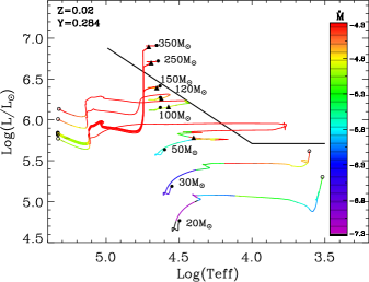
Since for the most massive stars at solar metallicity this may happen near the Humphreys-Davidson limit, the above formalisms could provide a modern description of the transition from O-type through LBV/RSG-type to WR-types (Vink & Gräfener, 2012). We thus include in PARSEC the recent formulation of mass-loss rates by Vink et al. (2011). The resulting HR diagram of a few selected evolutionary tracks for about solar metallicity is shown in the upper panel of figure 1. For purposes of clearness, we do not plot the pre-main sequence phase. The colours along the tracks represent the strength of the mass-loss rates as indicated in the inset scale. In the figure, the thick black lines mark the so-called Humphreys-Davidson limit (Humphreys & Davidson, 1979) which delimit the forbidden region above which only very few stars are observed in the HR diagram of the Galactic massive stars. As shown in the figure, the main sequence of the most massive stars extends up to the Humphreys-Davidson limit. Eventually, the stars may encompass this limit but the time spent in this region is very short because the mass-loss rate becomes so high that the stars rapidly lose their envelopes and turn into the hotter region of the HR diagram. We stress that this is not a result of an ad hoc assumption for the mass-loss rate, but a direct result of the application of the new adopted relations of the mass-loss rates. Near the Humphreys-Davidson limit, $\Gamma_{e}$ rises close to 1 and, as described in Vink et al. (2011), when $\Gamma_{e}$ is larger than 0.7, the mass-loss dependence on $\Gamma_{e}$ becomes high and, correspondingly, the mass-loss rates are significantly enhanced. With this formulation, the boosting of the mass-loss rate at the highest masses ($M_{\rm ini}$$\geq 150M_{\odot}$) is effective already from the beginning of the main sequence and, because of the large mass-loss rates, they evolve almost downward vertically in the HR diagram. Interestingly, the luminosity of the tracks with the higher masses ($M_{\rm ini}$$\geq 150M_{\odot}$) falls with time much more than those of the less massive ones. This is caused by the over-luminosity with respect to the main sequence mass – luminosity relation which, being larger at larger masses, results in larger values of $\Gamma_{e}$. Thus, the evolved brightest massive stars are not necessarily those with the largest initial masses.

The $\Gamma_{e}$ dependence of the mass-loss rates of O-type supergiant stars has not yet been studied for different galactic environmental conditions, apart from the analysis of the effects of CNO abundances (Muijres et al., 2012a). A more thorough analysis in a broad metallicity range, $10^{-3}~{}Z_{\odot}\leq~{}Z\leq~{}2~{}Z_{\odot}$, has been performed by Gräfener & Hamann (2008), but only for the case of WR stars. In particular, Gräfener & Hamann (2008) show that the dependence of mass-loss rates on the metallicity is also a strong function of $\Gamma_{e}$. While at low values of $\Gamma_{e}$ the mass-loss rates obey the relation of $\dot{M}\propto(Z/Z_{\odot})^{0.85}M_{\odot}/yr$, at increasing $\Gamma_{e}$ the metallicity dependence decreases, and it disappears as $\Gamma_{e}$ approaches 1. In the absence of a more comprehensive analysis of the dependence of the mass-loss rates on the metallicity and $\Gamma_{e}$, and since there is a continuity between the models provided by Vink et al. (2011) and those of WNL stars provided by Gräfener & Hamann (2008) (see discussion in Vink et al. (2011)), we assume in PARSEC that the scaling with the metallicity obeys the following relation

$$\dot{M}\propto~{}(Z/0.02)^{\alpha}$$ (2)

with the coefficient $\alpha$ determined from a rough fit to the published relationships by Gräfener & Hamann (2008):

$$\alpha=2.45-2.4*\Gamma_{e}\qquad(2/3\leq\Gamma_{e}<{1})$$ (3)

and with the supplementary condition $0<\alpha\leq{0.85}$. In summary, our algorithm for the mass-loss is the following. Besides the already specified mass-loss rate formulations (R_V01, R_dJ and R_NL) we compute also R${}_{\Gamma_{e}}$ from the tables provided by Vink et al. (2011), but we scale the latter value with the metallicity, using equations (2) and (3). During the BSGs and LBVs phases the basic mass loss rate adopted is R_V01. However, since, because of the effects of $\Gamma_{e}$, this can be encompassed by R${}_{\Gamma_{e}}$ and in order to secure a smooth transition, we adopt the maximum between R_V01 and R${}_{\Gamma_{e}}$. Toward the red supergiant phase we use R_dJ, but again, since this is an empirical rate parameterized in such a way that it should hold on a broad region of the HR diagram and it likely underestimates the mass loss rates of luminous yellow super-giants (Salasnich, Bressan & Chiosi, 1999), we compare it with R${}_{\Gamma_{e}}$ and take the maximum value. In the WR phases we consider the Nugis & Lamers (2000) formulation.

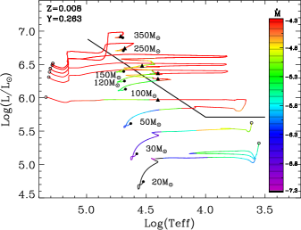
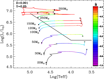
The HR diagram of a few selected evolutionary tracks for Z=0.008 is shown in the middle panel of figure 1. We note here a significant decrease of the mass-loss rates, at a given mass. In particular while at Z=0.02 the models of $M_{\rm ini}$$\sim$120M_⊙ and $M_{\rm ini}$$\sim$150M_⊙, rapidly turn their main sequence evolution to higher effective temperatures, at Z=0.008 the mass-loss rates are not high enough to prevent the tracks from entering into the forbidden region. Nevertheless, the tracks burn Hydrogen around the Humphreys-Davidson limit until, near central Helium ignition $\Gamma_{e}$ becomes large and after performing a rapid excursion within the forbidden region, they turn into the blue part as WR stars. At even lower metallicities, the mass-loss rates decrease, unless the star is near the Eddington limit with $\Gamma_{e}\sim$1, and the location of the predicted Humphreys-Davidson limit shifts to higher luminosities. For example, at Z=0.001 in the lower panel of figure 1, the upper main-sequence widens significantly and the more massive stars evolve into the “forbidden” region even during the H-burning phase, because of their very large convective cores. They may also ignite and burn central Helium as “red” supergiant stars.

2.4 Comparison with previous releases

The current set of massive stars supersedes the old one adopted in several popular studies since 20 years (Bressan et al., 1993; Fagotto et al., 1994, hereafter BF+). With respect to BF+, the new models have a significantly finer mass spacing and extend up to a higher upper mass limit. The computed masses range from 14 to 20 ${\rm~{}M_{\odot}}\,$in steps of 2 ${\rm~{}M_{\odot}}\,$, then up to 100 ${\rm~{}M_{\odot}}\,$in steps of 5 ${\rm~{}M_{\odot}}\,$and finally 120, 150, 200, 250, 300, 350 ${\rm~{}M_{\odot}}\,$. This allows for a quite better interpolation in ages and masses and a sampling of different initial mass function up to larger initial masses. Simple stellar populations can now be sampled with a higher accuracy than before and with more suitable mass and time-steps. The new tracks include also the pre-main sequence phase that begins when the central temperature of the protostar becomes larger than log(T${}_{c}/K)=5.3$. No mass accretion is accounted for during the pre-main sequence phase.

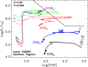
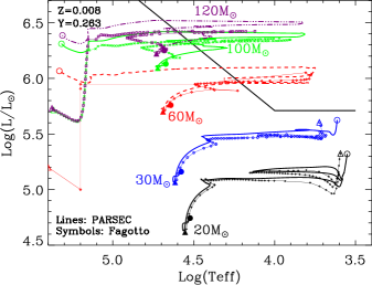
To summarize the differences brought by the adoption of the updated physics input we compare the new tracks with those of the previous Padova release, in the upper and middle panels of figure 2, for $Z=0.02$ and $Z=0.008$ respectively. Besides the presence of the pre-main sequence in the new tracks, which for purposes of clarity is not shown, a few general trends can be seen in the figure. At Z=0.02, the Zero Age Main Sequence (ZAMS) is similar. Note that the old tracks do not include the pre-main sequence phase. The main sequence termination is only slightly hotter in the new tracks, likely because of differences in the underlying opacities. The red supergiant phase is slightly cooler in the new tracks, but the differences are barely significant. We remind that in BF+ the density inversion (arising in the inefficient region of the convective envelope) was inhibited in the computation of massive star tracks. In a later revision of the tracks (Girardi et al., 2000) it was inhibited at all masses. As discussed in Alongi et al. (1993), a density inversion may develop in the external inefficient convection zones because of the requirement of the hydrostatic equilibrium in a region with a large super-adiabatic real temperature gradient (assuming typical values of the mixing length parameter). This situation which should lead to a Rayleigh-Taylor instability or even a significant increase in the mass-loss rate, may give rise to numerical instabilities which preclude the computation of the track. To inhibit the density inversion one may use a mixing length parameter proportional to the density scale height ($H_{\rho}$) which, by rendering convection more efficient in the region where the density has a relative maximum, prevents a large super-adiabatic real temperature gradient. Alternatively one may impose that the real temperature gradient is limited by $\nabla_{T}\leq\nabla_{T_{\rm max}}=\frac{1-\chi_{\mu}\nabla_{\mu}}{\chi_{T}}$, which is the choice made since BF+. This also simulates a more efficient convection and prevents the development of numerical instabilities. However since a larger convective efficiency results in a hotter red giant track, and since BF+ red giant tracks of intermediate and low mass stars compared well with the corresponding observed colours, we follow their method and inhibit density inversion only for the most massive stars. Thus the most massive red super-giants have effective temperatures that are slightly hotter than those obtained by allowing density inversion to occur. A detailed analysis of this effect is clearly needed, but likely it must also take into account effects of dusty circumstellar envelopes which are known to affect the colours of RSG stars.

The mass-loss rates adopted here are less efficient already at $M_{\rm ini}$=30 ​${\rm~{}M_{\odot}}\,$. At this mass, the star ignites Carbon as a red giant while in BF+ the star is already moving toward the hot region of the HR diagram. This effect is more striking in the more massive stars, for those reaching the WR stages. Comparing the two models of 60 ${\rm~{}M_{\odot}}\,$we see that while the H-burning and the central Helium ignition phases are pretty similar, the final WR phase is very different. The mass-loss adopted for the WR stages in BF+ is significantly larger than that adopted here and the star ends with a luminosity which is about one order of magnitude lower.

Figure 3: Upper panel: comparison of WM-basic spectra (smoothed) with different mass-loss rates. The effective temperature, gravity, radius and metallicity ($Z=0.02$) are the same, but the black solid line is for $\dot{M}=10^{-5}M_{\odot}\ yr^{-1}$ and the red dotted line is for $\dot{M}=10^{-7}M_{\odot}\ yr^{-1}$. The ionizing photon (with wavelength less than $912~{}{\rm nm}$) number ratio ($N_{\rm Ionizing}(\dot{M}=10^{-5}M_{\odot}\ yr^{-1})/N_{\rm Ionizing}(\dot{M}=10^{-7}M_{\odot}\ yr^{-1})$ supposing the same luminosity) is 0.197.      Lower panel: comparison of WM-basic spectra (smoothed) with different metallicities. The effective temperature, gravity, radius and mass-loss rate ($\dot{M}=10^{-5}M_{\odot}\ yr^{-1}$) are the same, but the black solid line is for $Z=0.02$ and the red dotted line is for $Z=0.008$. The ionizing photon number ratio ($N_{\rm Ionizing}(Z=0.02)/N_{\rm Ionizing}(Z=0.008)$ supposing the same luminosity) is 0.994 (almost identical). All the spectra are normalized over the wavelength range from 0.84 to 1.44 $\micron$.

At higher masses, $M_{\rm ini}$=100 and 120 ${\rm~{}M_{\odot}}\,$, there are significant differences already in the core H-burning. The mass-loss rates are initially higher in the BF+ models, but when the effects of $\Gamma_{e}$ become important, the mass-loss rates become comparable and the tracks evolve along the similar path. There remain a large difference in the mass-loss rate adopted in the advanced WR stages.

We stress again that in BF+ models the mass-loss is arbitrarily enhanced when the stars approach or encompass the Humphreys-Davidson limit, while in the current models the mass-loss enhancement is a result of the photospheric conditions. In this respect, it is very interesting to note the similarity between the tracks of $M_{\rm ini}$=60 ${\rm~{}M_{\odot}}\,$that can be taken as representative of the fact that the mass-loss enhancement is no more imposed as before, but it is instead a natural consequence of the photospheric conditions.

The comparisons with the models of Z=0.008, typical of the Large Magellanic Cloud, confirm the previous picture. The ZAMS is pretty similar, but now the effects of a lower metallicity become visible, since the normalization metallicity for the mass-loss rate has been assumed to be Z=0.02. In the old models, the metallicity dependence was slightly lower, $\dot{M}\propto~{}(Z/0.02)^{0.5}$, and the mass-loss rates at Z=0.008 were about 40% larger than in the current models, keeping other parameters fixed. Thus, the new models evolve at slightly higher luminosity until the effects of $\Gamma_{e}$ become important. Again there is a striking similarity in the turnover of the effective temperature in the models that overcome the Humphreys-Davidson limit. As before, in the final WR stages the stars evolve at a significantly higher luminosity than that of the old models. We note that, while in the advanced WR stages the luminosities of the new models are significantly higher, the corresponding lifetime is more or less unchanged ($\sim 0.1\,{\rm Myr}$ for $100\,\mbox{$M_{\odot}$}$ models). This means that the new models should contribute far more to the hard ionizing photons than the old ones. This will be the subject of a forthcoming paper dedicated to the integrated properties of young star clusters.

Figure 4: Evolutionary tracks for massive stars with Z=0.02 (left panel) and Z=0.008 (right panel). Different colours represent different evolutionary stages: black dotted lines for stages precedent of WR phases, red solid lines for models using PoWR WNL-H50 ($Z=0.02$) or WNL-H40 ($Z=0.008$), blue dash-dotted lines for WN models, and brown dashed lines for WC models. The meaning of big circles is the same as in figure 1. The overplotted vertical lines delimit the coverages of different atmosphere models as indicated in the plots. The Humphreys-Davidson limit is also drawn as in figure 1.

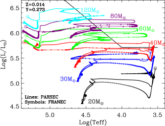
For the comparison with models by other groups, we select the evolutionary tracks without rotation computed with the FRANEC code (Chieffi & Limongi, 2013). The HR diagram is shown in the lower panel of figure 2. The FRANEC models (dashed lines) are for a composition of $Z=0.01345$ and $Y=0.265$ while PARSEC models (solid lines) are for a slightly different chemical composition, $Z=0.014$ and $Y=0.273$. They adopt a mixing-length parameter $\alpha\equiv\Lambda/H_{p}=2.3$ and a core overshooting region of $0.2H_{p}$ (Chieffi & Limongi, 2013; Martins & Palacios, 2013). One of the major difference is the presence of big blue loops in the FRANEC $20\,,30$ and $40\,\mbox{$M_{\odot}$}$ models, while the big blue loops are absent in our models. In this respect, we note that the main sequence termination of our models is significantly cooler and more luminous than that of FRANEC models. This is particularly evident in the model of $M_{\rm ini}$=$40\,\mbox{$M_{\odot}$}$ and it is indicative of a larger central mixing during the main sequence phase of our models, which is known to disfavour the occurrence of blue loops. The larger extension of the loops in the FRANEC models could also be due to their use of the Ledoux criterion for the definition of the borders of the intermediate unstable regions. It is well known that the Ledoux criterion inhibits the development of the intermediate convective regions within the Hydrogen profile, at the end of the H-burning phase, favouring a deeper penetration of the convective envelope when the stars move into the RSG region. This is an important issue deserving further investigation. Preliminary models computed adopting either the Schwarzschild or the Ledoux criterion in the Hydrogen chemical composition profile, confirm that the main cause of the inhibition of blue loops is the extent of core overshooting (or another kind of extended mixing) during main Hydrogen burning phase. With a slightly reduced core overshooting, also PARSEC models with the Schwarzschild criterion show extended blue loops (Tang et al. 2015 in preparation).

We also see that the behavior of the tracks within the Humphreys-Davidson region is very similar. In both cases, the models abandon this forbidden region after losing a significant fraction of their mass. In both cases, the mass-loss must be enhanced, but the invoked mechanism are different: Chieffi & Limongi (2013) invoke the dust mass-loss enhancement (van Loon et al., 2005), while we invoke the $\Gamma_{e}$ mass-loss enhancement.

3 Stellar atmosphere models

We convert from effective temperature, gravity and luminosity to magnitudes and colours using theoretical atmosphere models. Since one of our aims is to provide also isochrones in the observational plane, we need a full set of atmosphere models encompassing a wide range of parameters, i.e. masses, evolutionary stages and metallicities. In the following, we describe the different atmosphere models adopted. We begin with ATLAS models (Kurucz, 1993; Castelli & Kurucz, 2004), which are the canonical models suitable for intermediate and low mass stars. We complement this library with our new calculations of wind models for hot massive stars with the WM-basic code (Pauldrach, Puls & Kudritzki, 1986), and new models of WR stars from the Potsdam group (Gräfener, Koesterke & Hamann, 2002; Hamann & Gräfener, 2003, 2004; Sander, Hamann & Todt, 2012; Hamann, Gräfener & Liermann, 2006; Hainich et al., 2014). For the coolest stars we adopt the Phoenix models (Allard et al., 1997), already extensively discussed in our previous paper (Chen et al., 2014).

3.1 Intermediate mass and low mass stars

The core of our library consists of the plane parallel ATLAS9 models (Kurucz, 1993). These LTE (Local thermal equilibrium) models are well suited to describe the atmospheres of intermediate and low mass stars of spectral type between A and K. The most recent ATLAS9 models are those computed by Castelli & Kurucz (2004). ATLAS9 models are based on the solar abundances by Grevesse & Sauval (1998) and make use of an improved set of molecular lines including TiO, $\rm H_{2}O$, HI-Hi and $\rm HI-H^{+}$. The model grids are computed for $\rm T_{eff}$ from 3500 K to 50000 K, $log\,{\rm g}$ from 0.0 dex to 5.0 dex and [M/H]=+0.5, +0.2, 0.0, -0.5, -1.0, -1.5, -2.0, -2.5, -3.5, -4 and -5.5. We limit the use of ATLAS9 models to the temperature range of 19000 K$>\rm T_{eff}>$6000 K. At higher temperature in general we need to consider models with mass-loss while at lower temperature the Phoenix models are more appropriate.

3.2 Hot massive stars

O, B stars.  For temperatures typical of O and B stars (60000 K$>\rm T_{eff}>$19000 K) we have generated a new library of models using the public code WM-basic (Pauldrach, Puls & Kudritzki, 1986). This allows us to take into account both the effects of extended winds and those of non-LTE, since both effects may significantly affect the emergent spectra of hot stars. We have generated new sets of stellar spectral libraries covering as much as possible the space of parameters of our new evolutionary tracks of massive stars, i.e. effective temperature, gravity, metallicity and mass-loss rate. The temperature grid ranges from $log\,{\rm T_{\rm eff}}=4.3$ to $5.0$ in steps of $\Delta log\,{\rm T_{\rm eff}}=0.025$  dex. At each temperature, we adopt a step in gravity of $\Delta log\,{\rm g}=0.5$ dex, with upper and the lower boundaries that depend on the $\rm T_{eff}$. Indeed, the highest gravity is determined by the fact that the line driven radiation force cannot initiate the stellar wind, while the lowest value corresponds to stability problems when the models approach the Eddington limit. At each grid point we consider three different values of the mass-loss rates, $\dot{M}=10^{-7}$, $10^{-6}$, and $10^{-5}\,M_{\odot}/yr$, encompassing typical values for O, B stars.

Figure 5: Colour-magnitude diagrams in HST/WFC3 broad bands for tracks of $M_{\rm ini}$=$150M_{\odot}$ (upper four panels) and $M_{\rm ini}$=$50M_{\odot}$ (lower four panels) with Z=0.02 (left panels) and Z=0.008 (right panels) respectively. The meaning of colours and line styles along the tracks is the same as in figure 4. The meaning of big circles is the same as in figure 1.

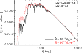
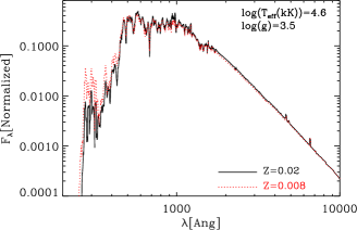
We note that, besides $\rm T_{eff}$, $log\,{\rm g}$ and stellar radius (radius defined at a Rosseland optical depth of $2/3$, $R_{*,2/3}$), there are additional input parameters in WM-basic, $\kappa$, $\alpha$ and $\delta$, referring most specifically to the structure of the wind as shown by Castor, Abbott & Klein (1975). Thus, for any point in the (effective temperature, gravity) grid we suitably change the other stellar parameters (radius, luminosity and mass) as well as the wind parameters $\alpha$ and $\kappa$ in order to obtain three consistent atmosphere models with the required values of mass-loss rate, $\dot{M}=10^{-7},10^{-6},10^{-5}M_{\odot}/yr$. These models are used to derive the broad band colours and magnitudes for any given effective temperature, gravity and metallicity, easily interpolating for the different values of the mass-loss rate actually used in the tracks. Our new library consists of about 300 models for each metallicity. For example for $z=0.02$, we computed 105 models for $\dot{M}=10^{-7}M_{\odot}\ yr^{-1}$, 98 for $\dot{M}=10^{-6}M_{\odot}\ yr^{-1}$ and 86 for $\dot{M}=10^{-5}M_{\odot}\ yr^{-1}$. The metal partition adopted in the new models is the same as used in Bressan et al. (2012), to say Caffau et al. (2011). As an example, we show in figure 3, the effects of changing the mass-loss rate at constant metallicity (upper panel) and those of changing the metallicity at constant mass-loss rate (lower panel), for models with $log\,{\rm T_{\rm eff}}=4.6$ and $log\,{\rm g}=3.5$. In the upper panel, the black solid line refers to the model with $\dot{M}=10^{-5}M_{\odot}\ yr^{-1}$, while the red dotted one is for $\dot{M}=10^{-7}M_{\odot}\ yr^{-1}$. We can see that the ${\rm He\,II}$ continuum is more absorbed in the model with higher mass-loss rate. We notice also that, as expected, some spectral features which appears in emission in the higher mass-loss rate model, turn into absorption in the model with a lower mass-loss rate.

In the lower panel, the black solid line refers to the same model as in the upper panel, while, the red dotted one is now for a model at the same grid point but with $Z=0.008$. This comparison shows that the effects of changing the metallicity on these hot spectra are less pronounced than those arising from the variation of the mass-loss rates.

Wolf-Rayet stars.  WR stars typically have wind densities one order of magnitude larger than those of massive O-type stars. Spectroscopically they are dominated by the presence of strong broad emission lines of Helium, Nitrogen, Carbon and Oxygen. They are subdivided into different sub-types, one with strong lines of Helium and Nitrogen (WN stars), another one with strong lines of Helium and Carbon (WC stars) and a third one with strong Oxygen lines (WO stars).

To reproduce their spectra we make use of the most recent library of WR models computed by the Potsdam group (PoWR) (Gräfener, Koesterke & Hamann, 2002; Hamann & Gräfener, 2003, 2004; Sander, Hamann & Todt, 2012; Hamann, Gräfener & Liermann, 2006; Hainich et al., 2014). They provide models with metallicities corresponding to those of WR stars in the Galaxy, the LMC and the Small Magellanic Cloud (SMC). The model grids are parameterized with ${\rm T_{eff,\tau=20}}$ (the effective temperature at radius where the Rosseland optical depth is 20), and the transformed radius $R_{t}$ (because models with the same set of such parameters show the same emergent spectrum as discussed in Schmutz, Leitherer & Gruenwald (1992)). The transformed radius $R_{t}$ is given by (Schmutz, Hamann & Wessolowski, 1989):

$$R_{t}=R^{*}_{\tau=20}\Biggl{(}\frac{v_{\infty}}{2500\,km\,s^{-1}}\frac{10^{-4}M_{\odot}yr^{-1}}{\dot{M}}\Biggr{)}^{{\color[rgb]{0,0,0}2/3}}.$$ (4)

Since $R^{*}_{\tau=20}$ is nearly equivalent to the hydrostatic radius of the evolutionary tracks, this quantity combines stellar radius and mass-loss rate of the tracks with the terminal velocity. For the same reason ${\rm T_{eff,\tau=20}}$ corresponds to the effective temperature of our hydrostatic models $\rm T_{eff}^{*}$. As shown in Hamann & Gräfener (2004), at large $R_{t}$ (or thin winds), ${\rm T_{eff,\tau=20}}\backsimeq{\rm T_{eff,\tau=2/3}}$. (In the case of our WM-basic models, $R_{t}$ are always $\gtrsim 1.5$, so there is no need to use $R_{t}$ to match atmosphere models and theoretical tracks). As done in Schmutz, Leitherer & Gruenwald (1992), we match the WR atmospheres to the evolutionary tracks by interpolating $\rm T_{eff}^{*}$ and $R_{t}$.

Figure 6: Comparison of CMFGEN (Hillier & Miller, 1998) WC and WN models with the same effective temperature $\rm T_{eff}=120000\,K$ and metallicity Z=0.02. Also shown are the transmission curves of three HST/WFC3 filters (F438W, F555W and F814W). Notice that the two strong emission lines HeII(4700) and CIV(5800) can greatly influence the magnitude/colours in related passbands.

While the observational classification is quite well defined (Crowther, 2007; Crowther, De Marco & Barlow, 1998), it is more difficult to assign the WR subgroups along the evolutionary tracks. We use the following convention to identify them. WR stars are classified as WNL (late) when the surface Hydrogen mass fraction $X_{H}$ is below a given threshold, X_WNL. When $\rm X_{H}=0$, they are classified as WNE (early) if $N(^{12}{\rm C})<N(^{14}{\rm N})$ and as WC if $N(^{12}{\rm C})\geq N(^{14}{\rm N})$. We finally assign the WO subtype when the condition $N(^{12}{\rm C})+N(^{16}{\rm O})>N(^{4}{\rm He})$ is fulfilled (Smith & Maeder, 1991). We then match our type assignments with the models provided by PoWR, which adopt a fixed composition for any given subtype. For example, for the Galactic metallicity, in the PoWR library X_WNL=0.5 and the different subtypes have the following surface compositions:

• WNL-H50 for $X_{\rm H}\!=\!X_{\rm WNL}$, $X_{\rm He}\!=\!0.48$, $X_{\rm C}\!=\!{\rm 1E\!-\!4}$, $X_{\rm N}\!=\!0.015$, $X_{\rm O}\!=\!0$ and $X_{\rm Fe}\!=\!0.0014$;

• WNL for $X_{\rm H}\!=\!0.2$, $X_{\rm He}\!=\!0.78$, $X_{\rm C}\!=\!{\rm 1E\!-\!4}$, $X_{\rm N}\!=\!0.015$, $X_{\rm O}\!=\!0$ and $X_{\rm Fe}\!=\!0.0014$;

• WNE for $X_{\rm H}\!=\!0$, $X_{\rm He}\!=\!0.98$, $X_{\rm C}\!=\!{\rm 1E\!-\!4}$, $X_{\rm N}\!=\!0.015$, $X_{\rm O}\!=\!0$ and $X_{\rm Fe}\!=\!0.0014$;

• WC for $X_{\rm H}\!=\!0$, $X_{\rm He}\!=\!0.55$, $X_{\rm C}\!=\!0.4$, $X_{\rm N}\!=\!0$, $X_{\rm O}\!=\!0.05$ and $X_{\rm Fe}\!=\!0.0016$.

For the LMC, the surface Hydrogen threshold is X_WNL=0.4, while for the SMC they provide models with both X_WNL=0.6 (WNL-H60 models) and X_WNL=0.4 (WNL-H40 models). Note that PoWR does not yet provide spectral models for WO stars, which, however, are quite rare objects especially at lower metallicities.

Figure 7: Isochrones of different ages, as indicated by the labels, are shown for Z=0.02 (left panel) and Z=0.008 (right panel). Note that at young ages the intermediate and low mass stars are still on the pre-main sequence (grey dotted lines). The Humphreys-Davidson limit is also drawn as in figure 1.

Figure 8: Colour-magnitude diagrams in HST/WFC3 broad bands for isochrones of 1 Myr (upper four panels) and 2.5 Myr (lower four panels) with Z=0.02 (left panels) and Z=0.008 (right panels). The meaning of colours and line styles along the isochrones is the same as in figure 4.

3.3 Cool stars

As reviewed by Allard et al. (1997), the atmospheres of cool stars are dominated by the formation of molecules and eventually at very low temperatures by dust condensation that can affect the spectral shape significantly. A suitable set of 1D, static spherical atmosphere spectral models accounting for the above effects has been developed in the recent years and is continuously maintained by the Phoenix group (Allard et al., 2012). Among the different suites of libraries, we use the BT-Settl models which contain the most updated and complete stellar parameter grid and are well tested against observations (Allard et al., 2012). The full BT-Settl models are provided for $2600\,$K $\leq\rm T_{eff}<50000\,K$, $0.5<log\,{\rm g}<6$, and metallicities $0.000003\lesssim Z\lesssim 0.04$. We adopt such models for temperatures $\rm T_{eff}\leq 6000\,K$. These tables for cool stars have already been used in Chen et al. (2014), in the context of low and very low mass stars.

3.4 Synthetic bolometric correction tables

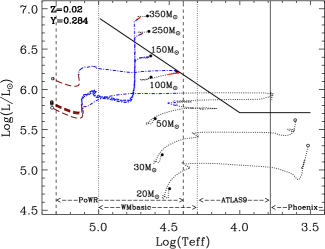
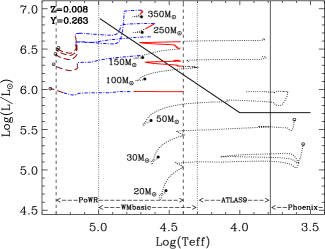
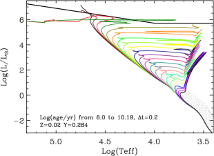
A concern for the libraries described above is that the different sets (WM-basic, PoWR, ATLAS9 and BT-Settl) are calculated with different metallicities and different partitions of heavy elements. In order to obtain homogeneous spectral libraries, at least as far as the metallicity is concerned, we first calculate the global metallicity from the detailed abundance values provided by each group. We note, for example, that the BT-Settl models adopt a solar partition (Asplund et al., 2009) different from the one adopted in PARSEC (Caffau et al., 2011) and that, at low metallicities, their partitions are $\alpha$ enhanced. On the contrary, for our WM-basic models, we use the same metallicities as in PARSEC. We then interpolate each set of spectra on the global metallicity grid defined by the PARSEC models. Since PoWR models are provided only for three typical metallicities, our Galaxy, the LMC and the SMC, we use Galaxy models for $Z\geqslant 0.01$, LMC models for $0.01>Z>0.006$ and SMC models for $Z\leqslant 0.006$. Unfortunately this procedure may introduce some error because the partition of heavy elements is not the same in the different libraries. For example when we re-scale the Caffau et al. (2011) and the Grevesse & Sauval (1998) partitions to a metallicity of Z=0.02, we find a difference of $\sim$17% in the Iron content and $\sim$5% in the Oxygen content. However we verified that these variations have negligible effects on the broad band colours of hot spectra. On the other hand this is the best one can do until a homogeneous set of model atmospheres (i.e. with the same partition of heavy elements) is computed on a range of parameters broad enough. The ranges of effective temperatures encompassed by different spectral libraries are marked by vertical lines in the HR diagrams shown in figure 4, for $Z=0.02$ (left panel) and $Z=0.008$ (right panel), respectively. Overplotted are selected stellar evolutionary tracks from $M_{\rm ini}$=$20\,M_{\odot}$ to $M_{\rm ini}$=$350\,M_{\odot}$. The combined atmosphere models, that share the same global metallicity of the corresponding evolutionary tracks as shown in the HR diagram, provide a very good coverage in terms of effective temperatures and gravities. They allow for an optimal calculation of bolometric correction (${\rm BC_{\lambda}}$) tables that are used to convert from theoretical to observational diagrams. The details of this process are thoroughly described in Girardi et al. (2002) and Chen et al. (2014), and are not repeated here. While for the evolutionary tracks we only consider the photospheric magnitudes, the corresponding isochrones also account for the effect of possible circumstellar dusty envelopes following the dust calculation recipes described in Marigo et al. (2008) and  Nanni et al. (2013, 2014).

4 Discussions and Conclusions

We present new evolutionary tracks of massive stars for a broad range of metallicities, 0.0001 $\leq~{}Z~{}\leq 0.04$ and for initial masses up to $M_{\rm ini}$=$350\mbox{$M_{\odot}$}$. At super-solar metallicity, the models extend up to $M_{\rm ini}$=$200\mbox{$M_{\odot}$}$ (Z=0.03) and $M_{\rm ini}$=$150\mbox{$M_{\odot}$}$ (Z=0.04), respectively. The new models complement the already published PARSEC data base (Bressan et al., 2012) and supersede the old Padova evolutionary tracks of massive stars which are more than 20 years old. The stellar models are evolved from the pre-main sequence phase to the central Carbon ignition. The mass grid is very well sampled and it is fully adequate to perform detailed investigations of very young stellar systems both from the point of view of the resolved populations and from their integrated properties.

We revise the scheme adopted for including the mass-loss rate in the evolution of massive stars, by combining recent recipes found in the literature. Among the new recipes, particularly important is the enhancement of the mass-loss rate when the luminosity approaches the Eddington limit. We show that with the recent formulation by Vink et al. (2011), the models naturally reproduce the observed Humphreys-Davidson limit observed in the Galactic and LMC HR diagrams. In previous Padova models this limit was used as a threshold to enhance the mass-loss rates, independently from the metallicity. In this paper, the role of the metallicity is described by means of a simple recipe derived from the models presented in Gräfener & Hamann (2008). The metallicity dependence of the mass-loss rate is now described by a power law with an exponent $\alpha$ which depends on $\Gamma_{e}$ (equation (1)), the ratio between the stellar luminosity and the Eddington luminosity. When $\Gamma_{e}$ approaches unity the metallicity dependence drops significantly, allowing for relatively high mass-loss rates also in stars of low metallicity. At lower values of $\Gamma_{e}$ the usual exponent is recovered, $\alpha$=0.85. While the models of Gräfener & Hamann (2008) refer particularly to the WR phase, it has already been shown that there is a continuity between the new Vink et al. (2011) formalism and the Gräfener & Hamann (2008) results for WNL stars. The result of the new mass-loss formulation is that the Humphreys-Davidson limit shows a clear dependence with metallicity and it even disappears at very low metallicities.

Compared to our previous models with the same metallicity (Fagotto et al., 1994; Bressan et al., 1993), the major difference concerns the WR phases. The new models evolve in the late WR stage, at $log\,{\rm T_{\rm eff}}>5.0$, with luminosities which are significantly higher than those of the old Padova tracks ($\sim 0.9\,{\rm dex}$ in $\log(L/L_{\odot})$). These differences result from the different mass-loss recipes used in the advanced WR phases. Since the lifetimes of the models in this phase remain more or less the same, the new models should contribute much more to the hard ionizing photons. At lower metallicity, Z$\leq$0.008, the new mass-loss formulation introduces significant differences even in the earlier phases. Our models compare well with the recent evolutionary tracks of non-rotating stars of similar metallicity, computed with FRANEC (Chieffi & Limongi, 2013).

Besides evolutionary tracks, we provide new tables of bolometric corrections that allow for the conversion from the theoretical HR to the observed colour-magnitude diagrams. For this purpose, we assemble existing atmosphere libraries, ATLAS9, PoWR, Phoenix and new atmosphere models calculated on purpose with the WM-basic code. We merge the different libraries with interpolation on a global metallicity scale, providing quite homogeneous tables of bolometric corrections, at several metallicities.

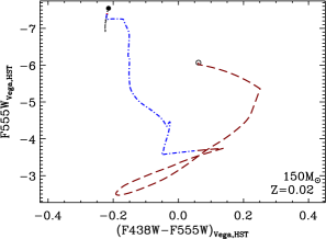
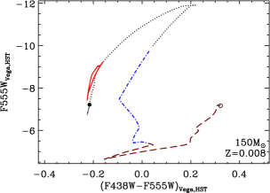
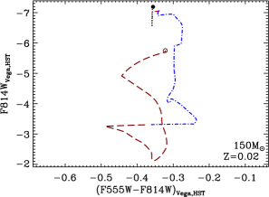
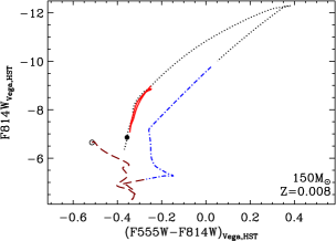
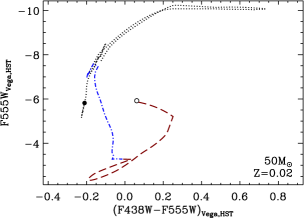
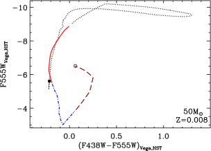
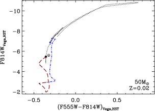
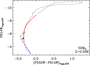
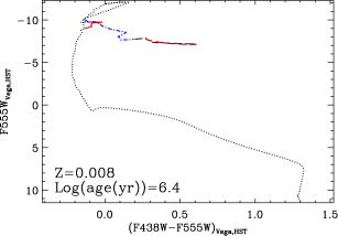
An example of the colour-magnitude diagrams of the tracks of $M_{\rm ini}$=$100M_{\odot}$ and $M_{\rm ini}$=$50M_{\odot}$ is shown in figure 5, for Z=0.02 (left panels) and Z=0.008 (right panels), respectively. In the figure, we highlight the different evolutionary phases with different colours and line styles. Black dotted lines indicate the evolution precedent of the WR stages, while the red solid lines are used to indicate the transition phase from the LBV phase to the late WR stars (WNL-H50 for $Z=0.02$ or WNL-H40 for $Z=0.008$ in the PoWR notation). The blue dash-dotted lines are used for the other WN stages and the brown dashed lines are for the final WC/WO stages.

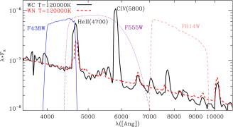
As can be seen in the figure, the optical colours show some evident jumps when the star type changes from WN to WC. This is likely to be caused by the appearance of different strong emission lines in different sub-types. This can be seen from figure 6, where we compare the spectra of one WC star (black solid line) and one WN (red dashed line) star with the same effective temperature. We show the optical region sampled by the broadband filters F438W, F555W, and F814W of the HST/WFC3 system. To better clarify this point we have used in the comparison the high resolution CMFGEN spectra (Hillier & Miller, 1998), which better show how the emission lines affect the spectra and the broadband colours. Both spectra show a strong emission HeII(4700Å) line, falling within the F555W passband and touching the border of the F438W passband. The differences between the WN and the WC spectral types are mainly on the contribution of the strong CIV(5800Å) line within the F555W passband, in the latter type. Thus, the flux in the F555W passband is heavily enhanced in the case of the WC star with respect to that of the WN star, and correspondingly the sudden transition from the WN to the WC types is accompanied by a jump in the F438W-F555W and F555W-F814W colours. It is important to stress that the CIV(5800Å) doublet is very sensitive to the adopted atmosphere parameters which somehow challenges its predictability (private communication with Helge Todt, Wolf-Rainer Hamann and Götz Gräfener). Furthermore, we have to note that the transition between WN and WC spectral types is smoother in the tracks than in the spectra, because the latter are computed only at discrete values of the elemental abundances, and this could enhance the effect, at least in terms of evolutionary speed.

Using the evolutionary tracks we compute new isochrones of young stellar populations, with the same procedure already described in Bressan et al. (2012). A few examples are shown in the theoretical HR diagram of figure 7, from very young to very old ages and for Z=0.02 (left panel) and Z=0.008 (right panel), respectively. By means of the new bolometric correction tables, we convert theoretical isochrones into observational magnitudes/colours, in the same way used for the evolutionary tracks. In figure 8 we show the colour-magnitude diagrams of isochrones at very young ages, 1 Myr and 2.5 Myr, and for Z=0.02 and Z=0.008. The colour codings are the same as in figure 5, but for the pre-main sequence which is drawn in light gray.

A preliminary comparison of the new models with the colour-magnitude diagrams of star-forming regions in nearby low metallicity dwarf irregular galaxies, has already been performed in Tang et al. (2014). The new models of massive stars will be used to compute the integrated properties of young star forming regions (Obi et al. in preparation). The full sets of evolutionary tracks can be downloaded from http://people.sissa.it/~sbressan/parsec.html. The isochrones can be downloaded from http://stev.oapd.inaf.it/cgi-bin/cmd.

References

- Allard et al. (1997) Allard F., Hauschildt P. H., Alexander D. R., Starrfield S., 1997, ARA&A, 35, 137
- Allard et al. (2012) Allard F., Homeier D., Freytag B., Sharp C. M., 2012, 57, 3
- Alongi et al. (1991) Alongi M., Bertelli G., Bressan A., Chiosi C., 1991, A&A, 244, 95
- Alongi et al. (1993) Alongi M., Bertelli G., Bressan A., Chiosi C., Fagotto F., Greggio L., Nasi E., 1993, A&AS, 97, 851
- Asplund et al. (2009) Asplund M., Grevesse N., Sauval A. J., Scott P., 2009, ARA&A, 47, 481
- Barsukova et al. (2014) Barsukova E. A., Goranskij V. P., Valeev A. F., Kaisin S. S., 2014, ArXiv e-prints
- Bertelli et al. (2009) Bertelli G., Nasi E., Girardi L., Marigo P., 2009, A&A, 508, 355
- Böhm-Vitense (1958) Böhm-Vitense E., 1958, ZAp, 46, 108
- Bressan et al. (1993) Bressan A., Fagotto F., Bertelli G., Chiosi C., 1993, A&AS, 100, 647
- Bressan et al. (2013) Bressan A., Marigo P., Girardi L., Nanni A., Rubele S., 2013, in European Physical Journal Web of Conferences, Vol. 43, European Physical Journal Web of Conferences, p. 3001
- Bressan et al. (2012) Bressan A., Marigo P., Girardi L., Salasnich B., Dal Cero C., Rubele S., Nanni A., 2012, MNRAS, 427, 127
- Bressan, Chiosi & Bertelli (1981) Bressan A. G., Chiosi C., Bertelli G., 1981, A&A, 102, 25
- Brott et al. (2011) Brott I. et al., 2011, A&A, 530, A115
- Bruzual & Charlot (2003) Bruzual G., Charlot S., 2003, MNRAS, 344, 1000
- Caffau et al. (2011) Caffau E., Ludwig H.-G., Steffen M., Freytag B., Bonifacio P., 2011, Sol. Phys., 268, 255
- Cai et al. (2014) Cai Z.-Y., Lapi A., Bressan A., De Zotti G., Negrello M., Danese L., 2014, ApJ, 785, 65
- Castelli & Kurucz (2004) Castelli F., Kurucz R. L., 2004, ArXiv Astrophysics e-prints
- Castor, Abbott & Klein (1975) Castor J. I., Abbott D. C., Klein R. I., 1975, ApJ, 195, 157
- Chen et al. (2014) Chen Y., Girardi L., Bressan A., Marigo P., Barbieri M., Kong X., 2014, MNRAS, 444, 2525
- Chieffi & Limongi (2013) Chieffi A., Limongi M., 2013, ApJ, 764, 21
- Crowther (2007) Crowther P. A., 2007, ARA&A, 45, 177
- Crowther, De Marco & Barlow (1998) Crowther P. A., De Marco O., Barlow M. J., 1998, MNRAS, 296, 367
- Cyburt et al. (2010) Cyburt R. H. et al., 2010, ApJS, 189, 240
- Dale, Ercolano & Bonnell (2012) Dale J. E., Ercolano B., Bonnell I. A., 2012, MNRAS, 424, 377
- Dale, Ercolano & Bonnell (2013) —, 2013, MNRAS, 430, 234
- de Jager, Nieuwenhuijzen & van der Hucht (1988) de Jager C., Nieuwenhuijzen H., van der Hucht K. A., 1988, A&AS, 72, 259
- Decressin et al. (2009) Decressin T., Mathis S., Palacios A., Siess L., Talon S., Charbonnel C., Zahn J.-P., 2009, A&A, 495, 271
- Deheuvels et al. (2010) Deheuvels S. et al., 2010, A&A, 514, A31
- Dewitt, Graboske & Cooper (1973) Dewitt H. E., Graboske H. C., Cooper M. S., 1973, ApJ, 181, 439
- Ekström et al. (2012) Ekström S. et al., 2012, A&A, 537, A146
- Fagotto et al. (1994) Fagotto F., Bressan A., Bertelli G., Chiosi C., 1994, A&AS, 104, 365
- Girardi et al. (2002) Girardi L., Bertelli G., Bressan A., Chiosi C., Groenewegen M. A. T., Marigo P., Salasnich B., Weiss A., 2002, A&A, 391, 195
- Girardi et al. (2000) Girardi L., Bressan A., Bertelli G., Chiosi C., 2000, A&AS, 141, 371
- Girardi, Rubele & Kerber (2009) Girardi L., Rubele S., Kerber L., 2009, MNRAS, 394, L74
- Graboske et al. (1973) Graboske H. C., Dewitt H. E., Grossman A. S., Cooper M. S., 1973, ApJ, 181, 457
- Gräfener & Hamann (2008) Gräfener G., Hamann W.-R., 2008, A&A, 482, 945
- Gräfener, Koesterke & Hamann (2002) Gräfener G., Koesterke L., Hamann W.-R., 2002, A&A, 387, 244
- Grevesse & Sauval (1998) Grevesse N., Sauval A. J., 1998, Space Sci. Rev., 85, 161
- Gustafsson et al. (2008) Gustafsson B., Edvardsson B., Eriksson K., Jørgensen U. G., Nordlund Å., Plez B., 2008, A&A, 486, 951
- Haft, Raffelt & Weiss (1994) Haft M., Raffelt G., Weiss A., 1994, ApJ, 425, 222
- Hainich et al. (2014) Hainich R. et al., 2014, A&A, 565, A27
- Hamann & Gräfener (2003) Hamann W.-R., Gräfener G., 2003, A&A, 410, 993
- Hamann & Gräfener (2004) —, 2004, A&A, 427, 697
- Hamann, Gräfener & Liermann (2006) Hamann W.-R., Gräfener G., Liermann A., 2006, A&A, 457, 1015
- Hillier & Miller (1998) Hillier D. J., Miller D. L., 1998, ApJ, 496, 407
- Hollenbach & Tielens (1999) Hollenbach D. J., Tielens A. G. G. M., 1999, Reviews of Modern Physics, 71, 173
- Humphreys & Davidson (1979) Humphreys R. M., Davidson K., 1979, ApJ, 232, 409
- Iglesias & Rogers (1996) Iglesias C. A., Rogers F. J., 1996, ApJ, 464, 943
- Itoh & Kohyama (1983) Itoh N., Kohyama Y., 1983, ApJ, 275, 858
- Itoh et al. (2008) Itoh N., Uchida S., Sakamoto Y., Kohyama Y., Nozawa S., 2008, ApJ, 677, 495
- Kamath et al. (2010) Kamath D., Wood P. R., Soszyński I., Lebzelter T., 2010, MNRAS, 408, 522
- Kato (1966) Kato S., 1966, PASJ, 18, 374
- Kennicutt (1998) Kennicutt, Jr. R. C., 1998, ARA&A, 36, 189
- Kimm & Cen (2014) Kimm T., Cen R., 2014, ApJ, 788, 121
- Komatsu et al. (2011) Komatsu E. et al., 2011, ApJS, 192, 18
- Kudritzki & Puls (2000) Kudritzki R.-P., Puls J., 2000, ARA&A, 38, 613
- Kurucz (1993) Kurucz R. L., 1993, in Astronomical Society of the Pacific Conference Series, Vol. 44, IAU Colloq. 138: Peculiar versus Normal Phenomena in A-type and Related Stars, Dworetsky M. M., Castelli F., Faraggiana R., eds., p. 87
- Lamers (1989) Lamers H. J. G. L. M., 1989, in Astrophysics and Space Science Library, Vol. 157, IAU Colloq. 113: Physics of Luminous Blue Variables, Davidson K., Moffat A. F. J., Lamers H. J. G. L. M., eds., pp. 135–146
- Ledoux (1947) Ledoux P., 1947, ApJ, 105, 305
- Mackey et al. (2014) Mackey J., Langer N., Mohamed S., Gvaramadze V. V., Neilson H. R., Meyer D. M.-A., 2014, ASTRA Proceedings, 1, 61
- Marigo & Aringer (2009) Marigo P., Aringer B., 2009, A&A, 508, 1539
- Marigo et al. (2008) Marigo P., Girardi L., Bressan A., Groenewegen M. A. T., Silva L., Granato G. L., 2008, A&A, 482, 883
- Martins & Palacios (2013) Martins F., Palacios A., 2013, A&A, 560, A16
- Meynet et al. (2015) Meynet G. et al., 2015, A&A, 575, A60
- Meynet & Maeder (2000) Meynet G., Maeder A., 2000, A&A, 361, 101
- Mokiem et al. (2007) Mokiem M. R. et al., 2007, A&A, 473, 603
- Muijres et al. (2012a) Muijres L., Vink J. S., de Koter A., Hirschi R., Langer N., Yoon S.-C., 2012a, A&A, 546, A42
- Muijres et al. (2012b) Muijres L. E., Vink J. S., de Koter A., Müller P. E., Langer N., 2012b, A&A, 537, A37
- Munakata, Kohyama & Itoh (1985) Munakata H., Kohyama Y., Itoh N., 1985, ApJ, 296, 197
- Nanni et al. (2013) Nanni A., Bressan A., Marigo P., Girardi L., 2013, MNRAS, 434, 2390
- Nanni et al. (2014) —, 2014, MNRAS, 438, 2328
- Nugis & Lamers (2000) Nugis T., Lamers H. J. G. L. M., 2000, A&A, 360, 227
- Pauldrach, Puls & Kudritzki (1986) Pauldrach A., Puls J., Kudritzki R. P., 1986, A&A, 164, 86
- Paxton et al. (2011) Paxton B., Bildsten L., Dotter A., Herwig F., Lesaffre P., Timmes F., 2011, ApJS, 192, 3
- Puls, Springmann & Lennon (2000) Puls J., Springmann U., Lennon M., 2000, A&AS, 141, 23
- Salasnich, Bressan & Chiosi (1999) Salasnich B., Bressan A., Chiosi C., 1999, A&A, 342, 131
- Sander, Hamann & Todt (2012) Sander A., Hamann W.-R., Todt H., 2012, A&A, 540, A144
- Sarangi & Cherchneff (2015) Sarangi A., Cherchneff I., 2015, A&A, 575, A95
- Schaerer et al. (2011) Schaerer D., Hayes M., Verhamme A., Teyssier R., 2011, A&A, 531, A12
- Schmutz, Hamann & Wessolowski (1989) Schmutz W., Hamann W.-R., Wessolowski U., 1989, A&A, 210, 236
- Schmutz, Leitherer & Gruenwald (1992) Schmutz W., Leitherer C., Gruenwald R., 1992, PASP, 104, 1164
- Schneider, Ferrara & Salvaterra (2004) Schneider R., Ferrara A., Salvaterra R., 2004, MNRAS, 351, 1379
- Schwarzschild (1958) Schwarzschild M., 1958, Structure and evolution of the stars. Princeton University Press
- Smith & Maeder (1991) Smith L. F., Maeder A., 1991, A&A, 241, 77
- Smith (2009) Smith N., 2009, in Massive Stars: From Pop III and GRBs to the Milky Way, Livio M., Villaver E., eds., Space Telescope Science Institute Symposium Series No. 20, Cambridge University Press, pp. 187–198
- Smith (2014) —, 2014, ARA&A, 52, 487
- Smith & Owocki (2006) Smith N., Owocki S. P., 2006, ApJ, 645, L45
- Tang et al. (2014) Tang J., Bressan A., Rosenfield P., Slemer A., Marigo P., Girardi L., Bianchi L., 2014, MNRAS, 445, 4287
- Torres et al. (2014) Torres G., Vaz L. P. R., Sandberg Lacy C. H., Claret A., 2014, AJ, 147, 36
- van Loon et al. (2005) van Loon J. T., Cioni M.-R. L., Zijlstra A. A., Loup C., 2005, A&A, 438, 273
- Vink, de Koter & Lamers (2000) Vink J. S., de Koter A., Lamers H. J. G. L. M., 2000, A&A, 362, 295
- Vink, de Koter & Lamers (2001) —, 2001, A&A, 369, 574
- Vink & Gräfener (2012) Vink J. S., Gräfener G., 2012, ApJ, 751, L34
- Vink et al. (2011) Vink J. S., Muijres L. E., Anthonisse B., de Koter A., Gräfener G., Langer N., 2011, A&A, 531, A132
- Yu, Wang & Li (2015) Yu N., Wang J.-J., Li N., 2015, MNRAS, 446, 2566