A 125 GeV Fat Higgs at large tanβ𝛽\tan\beta

Arjun Menona,b and Nirmal Rajb
 
aInstitute of Mathematical Sciences, Taramani, Chennai, 600113, India
bInstitute of Theoretical Science, University of Oregon, Eugene, OR 97405
Abstract

In this article we study the viability of regions of large tanβ𝛽\tan\beta within the framework of Fat Higgs/λ𝜆\lambda-SUSY Models. We compute the one-loop effective potential to find the corrections to the Higgs boson mass due to the heavy non-standard Higgs bosons. As the tree level contribution to the Higgs boson mass is suppressed at large tanβ𝛽\tan\beta, these one-loop corrections are crucial to raising the Higgs boson mass to the measured LHC value. By raising the Higgsino and singlino mass parameters, typical electroweak precision constraints can also be avoided. We illustrate these new regions of Fat Higgs/λ𝜆\lambda-SUSY parameter space by finding regions of large tanβ𝛽\tan\beta that are consistent with all experimental constraints including direct dark matter detection experiments, relic density limits and the invisible decay width of the Z𝑍Z boson. We find that there exist regions around λ=1.25,tanβ=50formulae-sequence𝜆1.25𝛽50\lambda=1.25,\tan\beta=50 and a uniform psuedo-scalar 4 TeV<MA< 8superscriptsimilar-to4 TeVsubscript𝑀𝐴superscriptsimilar-to84\mbox{ TeV}\>\raisebox{-2.15277pt}{$\stackrel{{\scriptstyle\textstyle<}}{{\sim}}$}\>M_{A}\>\raisebox{-2.15277pt}{$\stackrel{{\scriptstyle\textstyle<}}{{\sim}}$}\>8 TeV which are consistent will all present phenomenological constraints. In this region the dark matter relic abundance and direct detection limits are satisfied by a lightest neutralino that is mostly bino or singlino. As an interesting aside we also find a region of low tanβ𝛽\tan\beta and small singlino mass parameter where a well-tempered neutralino avoids all cosmological and direct detection constraints.

1 Introduction

Weak scale supersymmetry (SUSY) remains a popular and elegant solution to the hierarchy problem of the Standard Model (SM) [1]. It provides a natural means to stabilize the electroweak scale against large quadratic corrections from higher scales. The fact that the Higgs boson was discovered to be light [2, 3], in accordance with SUSY’s predictions, encourages us to continue our search for signals of SUSY at the TeV scale.

In the Minimal Supersymmetric extension of the Standard Model (MSSM), the tree-level Higgs quartic couplings are fixed to be the gauge couplings which leads to the tree-level Higgs boson mass that is below that of the Z𝑍Z boson. Therefore, raising the Higgs boson mass to the observed value of 125 GeV at the LHC [2, 3] requires large corrections due to a heavy stop sector [4, 5, 6, 7, 8, 9, 10, 11, 12, 13, 14]. However, heavy stops lead to large corrections to the up-type soft SUSY breaking Higgs squared mass parameter which in turn leads to a large correction to the electroweak symmetry breaking (EWSB) condition. A delicate cancellation between these corrections and the Higgsino mass parameter is needed to stabilize the electroweak scale, which is generally considered unnatural. Therefore in the MSSM there exists a tension between the observed Higgs mass and the requirement that the model is natural.

The Next-to-Minimal Supersymmetric Standard Model (NMSSM) is the simplest extension of the MSSM that can address this tension. In the NMSSM, the Higgs sector is enlarged to include an extra gauge singlet that couples to the remaining MSSM Higgs doublets through a Yukawa coupling λ𝜆\lambda. λ𝜆\lambda contributes to the Higgs quartic at tree-level, and for large enough values, can raise the Higgs mass to the observed 125 GeV. Therefore the stops need not be too heavy, thereby improving the naturalness of the model. Moreover, in the general NMSSM (GNMSSM), an additional tadpole term for the gauge singlet can also facilitate EWSB [15].

For λ>0.7𝜆similar-to0.7\lambda\begin{array}[]{c}\sim\vspace{-21pt}\\ >\end{array}0.7 at the weak scale, renormalization group (RG) evolution usually leads to this coupling developing a Landau pole below the GUT scale. Refs. [16, 17, 18, 19, 20, 21] have provided explicit UV-completions for such low scale models, which we collectively call Fat Higgs models. Refs. [22, 23, 24, 25, 26, 27, 28, 29, 30, 31, 32, 33, 34] have studied the phenomenological implications of models with such large λ𝜆\lambda couplings, which we collectively call λ𝜆\lambda-SUSY models. For these models, they have found that the Higgs mass can easily be raised to the observed value while still keeping the spectrum natural. These studies have focused on a region of low tanβ𝛽\tan\beta (vu/vdabsentsubscript𝑣𝑢subscript𝑣𝑑\equiv v_{u}/v_{d}, where vusubscript𝑣𝑢v_{u} and vdsubscript𝑣𝑑v_{d} are the vacuum expectation values (VEVs) of the corresponding Higgs doublets) and large λ𝜆\lambda because these regions were the most natural.

In this paper, we study the possibility of raising the Higgs mass to 125 GeV in Fat Higgs/λ𝜆\lambda-SUSY models at large tanβ𝛽\tan\beta. As the λ2superscript𝜆2\lambda^{2}-proportional tree-level contribution to the Higgs quartic is suppressed at large tanβ𝛽\tan\beta, the one-loop induced radiative corrections are crucial in raising the Higgs boson mass to its observed value. Similar to the stop-induced corrections that are proportional to yt4log(mt~2/Q2)superscriptsubscript𝑦𝑡4superscriptsubscript𝑚~𝑡2superscript𝑄2y_{t}^{4}\log(m_{\tilde{t}}^{2}/Q^{2}) (where ytsubscript𝑦𝑡y_{t} is the top Yukawa and mt~subscript𝑚~𝑡m_{\tilde{t}} is the stop mass scale), in Fat Higgs/λ𝜆\lambda-SUSY models the dominant one-loop corrections are proportional to λ4log(MA2/Q2)superscript𝜆4superscriptsubscript𝑀𝐴2superscript𝑄2\lambda^{4}\log(M_{A}^{2}/Q^{2}) (where MAsubscript𝑀𝐴M_{A} is the scale of the non-standard Higgs bosons). Therefore these corrections are only relevant when λ>1𝜆similar-to1\lambda\begin{array}[]{c}\sim\vspace{-21pt}\\ >\end{array}1 and the non-standard Higgs bosons are much heavier than the electroweak scale. The effect of radiative corrections in the NMSSM Higgs sector have been considered before [29, 35]. Ref. [29] focused on the most natural regions in the Scale-Invariant NMSSM, where it was found that these radiative corrections made a negligible contribution. In contrast, we show that at large tanβ𝛽\tan\beta, the λ𝜆\lambda induced radiative corrections can significantly modify the allowed regions of parameter space. Unlike Refs. [22, 29, 30], we also emphasize that electroweak precision constraints do not put a limit on tanβ𝛽\tan\beta. We point out that raising the Higgsino mass parameter μeffsubscript𝜇eff\mu_{\text{eff}} significantly weakens the electroweak precision constraints because the Higgsino component in the lightest neutralino is suppressed. The price of raising μeffsubscript𝜇eff\mu_{\text{eff}} is a slight increase in the tuning of the EWSB condition. To illustrate these effects in regions of large tanβ𝛽\tan\beta we also impose constraints from Higgs decay properties, direct dark matter detection experiments, the observed dark matter relic density and the invisible width of the Z𝑍Z boson. In particular, we find that direct dark matter detection experiments place strong limits on many regions of parameter space due to the large λ𝜆\lambda coupling. We also show that these allowed pockets of parameter space are within the reach of the XENON 1T experiment [36].

This paper is organized as follows. In Sec. 2, we set up the theoretical aspects required for the phenomenology of our model. To motivate the sizes of various terms in the Fat Higgs/λ𝜆\lambda-SUSY model, we present a “toy” high scale model where the fields have canonical mass dimensions in the electric theory. In addition, in this section we also compute the corrections to the Higgs quartic using the one-loop effective potential formalism, and discuss the Higgsino contributions to electroweak precision constraints and naturalness in the large tanβ𝛽\tan\beta regime of the Fat Higgs/λ𝜆\lambda-SUSY model. In Sec. 3, we illustrate the impact of the formalism in Sec. 2 by finding phenomenologically viable scenarios that can be probed at future experiments. In Sec. 4 we conclude.

2 Theoretical Setup

In this section we first motivate the form taken by our superpotential by a simple discussion of the sizes of various terms that can arise in Fat Higgs/λ𝜆\lambda-SUSY models. In this discussion we assume that any exotic fields are much heavier than the electroweak scale. For the superpotential thus obtained, we present the Higgs potential at the tree level and analytically compute the one-loop corrections to the mass of the SM-like Higgs boson due to heavy non-standard Higgs fields, with special attention to the limit of large λ𝜆\lambda and tanβ𝛽\tan\beta. In addition we discuss the naturalness of the large tanβ𝛽\tan\beta regions of the Fat Higgs/λ𝜆\lambda-SUSY models. We then discuss the reduced couplings of the SM-like Higgs to SM particles, which are constrained by LHC measurements of signal strengths. We end the section with a brief discussion of the neutralino sector with particular attention to electroweak precision observables.

2.1 Realizing low scale NMSSM with large λ𝜆\lambda

The GNMSSM with a large λ𝜆\lambda at the weak scale implies that some of the Higgs fields are composite states. For example, in the minimal Fat Higgs scenario of Ref. [16], all of the Higgs sector fields are composite, while in Refs. [17, 21] the MSSM Higgs fields are fundamental. For simplicity we will assume that at scales < 10superscriptsimilar-toabsent10\>\raisebox{-2.15277pt}{$\stackrel{{\scriptstyle\textstyle<}}{{\sim}}$}\>10 TeV, the only fields present in the Higgs sector are the SU(2)L𝑆𝑈subscript2𝐿SU(2)_{L} doublets H^u,H^dsubscript^𝐻𝑢subscript^𝐻𝑑\hat{H}_{u},\hat{H}_{d} and the gauge singlet S^^𝑆\hat{S}.111More exotic realizations typically require that additional Standard Model superfields are composite, introducing more exotic fields in the low energy theory [18, 19, 37, 38].

The most general superpotential with this particle content (assuming R-parity) has the form [43, 15]

𝒲GNMSSM=𝒲Yukawa+λS^H^uH^d+13κS^3+μH^uH^d+12μS^2+ξFS^,subscript𝒲GNMSSMsubscript𝒲Yukawa𝜆^𝑆subscript^𝐻𝑢subscript^𝐻𝑑13𝜅superscript^𝑆3𝜇subscript^𝐻𝑢subscript^𝐻𝑑12superscript𝜇superscript^𝑆2subscript𝜉𝐹^𝑆\displaystyle\mathcal{W}_{\rm GNMSSM}=\mathcal{W}_{\rm Yukawa}+\lambda\hat{S}\hat{H}_{u}\hat{H}_{d}+\frac{1}{3}\kappa\hat{S}^{3}+\mu\hat{H}_{u}\hat{H}_{d}+\frac{1}{2}\mu^{\prime}\hat{S}^{2}+\xi_{F}\hat{S}, (1)

where λ,κ𝜆𝜅\lambda,\kappa are dimensionless coupling strengths; μ,μ𝜇superscript𝜇\mu,\mu^{\prime} are supersymmetric mass terms; ξFsubscript𝜉𝐹\xi_{F} is a supersymmetric tadpole term of mass dimension 2, and 𝒲Yukawasubscript𝒲Yukawa\mathcal{W}_{\rm Yukawa} contains the standard MSSM Yukawa superpotential terms. The corresponding soft SUSY-breaking terms are

softsubscriptsoft\displaystyle-\mathcal{L}_{\rm soft} =\displaystyle= softf~+mHu2|Hu|2+mHd2|Hd|2+mS2|S|2+superscriptsubscriptsoft~𝑓superscriptsubscript𝑚subscript𝐻𝑢2superscriptsubscript𝐻𝑢2superscriptsubscript𝑚subscript𝐻𝑑2superscriptsubscript𝐻𝑑2limit-fromsuperscriptsubscript𝑚𝑆2superscript𝑆2\displaystyle-\mathcal{L}_{\rm soft}^{\tilde{f}}+m_{H_{u}}^{2}|H_{u}|^{2}+m_{H_{d}}^{2}|H_{d}|^{2}+m_{S}^{2}|S|^{2}+ (2)
(λAλHuHdS+13κAκS3+m32HuHd+12mS2S2+ξSS+h.c.),\displaystyle\left(\lambda A_{\lambda}H_{u}H_{d}S+\frac{1}{3}\kappa A_{\kappa}S^{3}+m_{3}^{2}H_{u}H_{d}+\frac{1}{2}{m^{\prime}_{S}}^{2}S^{2}+\xi_{S}S+h.c.\right),

where softf~superscriptsubscriptsoft~𝑓\mathcal{L}_{\rm soft}^{\tilde{f}} corresponds to the standard MSSM soft SUSY-breaking terms. mHu2,mHd2,mS2superscriptsubscript𝑚subscript𝐻𝑢2superscriptsubscript𝑚subscript𝐻𝑑2superscriptsubscript𝑚𝑆2m_{H_{u}}^{2},m_{H_{d}}^{2},m_{S}^{2} are the soft SUSY breaking Higgs squared mass terms and Aλ,Aκsubscript𝐴𝜆subscript𝐴𝜅A_{\lambda},A_{\kappa} are the soft SUSY breaking trilinear terms. m32,mS2superscriptsubscript𝑚32superscriptsubscriptsuperscript𝑚𝑆2m_{3}^{2},{m^{\prime}_{S}}^{2} are the CP-violating soft SUSY breaking squared mass terms and ξSsubscript𝜉𝑆\xi_{S} is the dimension-3 soft SUSY breaking term corresponding to ξFsubscript𝜉𝐹\xi_{F}.

A generic feature of most Fat Higgs/λ𝜆\lambda-SUSY models is that the Yukawa coupling λ>0.7𝜆similar-to0.7\lambda\begin{array}[]{c}\sim\vspace{-21pt}\\ >\end{array}0.7 at the TeV scale.222For Fat Higgs models that provide an existence proof of gauge coupling unification, see [16, 17]. Due to its renormalization group (RG) evolution, λ𝜆\lambda becomes stronger at higher scales and develops a Landau pole at the compositeness scale ΛHsubscriptΛ𝐻\Lambda_{H}, where ΛHsubscriptΛ𝐻\Lambda_{H} is assumed to be lower than the grand unification scale MGUTsubscript𝑀GUTM_{\rm GUT}. In the deep IR, much below ΛHsubscriptΛ𝐻\Lambda_{H}, the magnetic theory of mesons (i.e. the Higgs superfields) is described by the interactions in Eqs. (1) and (2). In the UV above ΛHsubscriptΛ𝐻\Lambda_{H}, some or all of the Higgs superfields are revealed to be composite states made up fundamental quarks whose interactions are described by some electric theory.

If the quarks in the electric theory have the canonical mass dimension and all Higgs superfields are composite, then the κ,μ,μ𝜅𝜇superscript𝜇\kappa,\mu,\mu^{\prime} terms in Eq. (1) and their corresponding soft SUSY-breaking terms in Eq. (2) are generated by marginal terms in the fundamental theory. This assumption is equivalent to saying that the confining dynamics only generates the λ𝜆\lambda term while all other couplings arise from non-renormalizable interactions in the electric theory. For example, in the simplest Fat Higgs model [16], the Higgs superfields in Eq. (1) are composite states of the quarks Tisubscript𝑇𝑖T_{i} in the electric theory. These quarks are charged under a confining SU(2)H𝑆𝑈subscript2𝐻SU(2)_{H} gauge group, thereby leading to the identification

S^T^5T^6;(H^u+H^u0)(T^1T^3T^2T^3);(H^d0H^d)(T^1T^4T^2T^4).formulae-sequencesimilar-to^𝑆subscript^𝑇5subscript^𝑇6formulae-sequencesimilar-tosuperscriptsubscript^𝐻𝑢superscriptsubscript^𝐻𝑢0subscript^𝑇1subscript^𝑇3subscript^𝑇2subscript^𝑇3similar-tosuperscriptsubscript^𝐻𝑑0superscriptsubscript^𝐻𝑑subscript^𝑇1subscript^𝑇4subscript^𝑇2subscript^𝑇4\displaystyle\hat{S}\sim\hat{T}_{5}\hat{T}_{6};\;\;\left(\begin{array}[]{c}\hat{H}_{u}^{+}\\ \hat{H}_{u}^{0}\end{array}\right)\sim\left(\begin{array}[]{c}\hat{T}_{1}\hat{T}_{3}\\ \hat{T}_{2}\hat{T}_{3}\end{array}\right);\;\;\left(\begin{array}[]{c}\hat{H}_{d}^{0}\\ \hat{H}_{d}^{-}\end{array}\right)\sim\left(\begin{array}[]{c}\hat{T}_{1}\hat{T}_{4}\\ \hat{T}_{2}\hat{T}_{4}\end{array}\right). (11)

The λ𝜆\lambda term in Eq. (1) is dynamically generated by the Pfaffian of the mesons in the magnetic theory. Naive dimensional analysis (NDA) [39, 40, 41] and canonical normalization of the fields (TiTj(ΛH/4π)ϕij)delimited-⟨⟩subscript𝑇𝑖subscript𝑇𝑗subscriptΛ𝐻4𝜋subscriptitalic-ϕ𝑖𝑗\left(\langle T_{i}T_{j}\rangle\to(\Lambda_{H}/4\pi)\phi_{ij}\right) lead to the relations

λ(ΛH)4π;similar-to𝜆subscriptΛ𝐻4𝜋\displaystyle\lambda(\Lambda_{H})\sim 4\pi; κ(ΛH)(ΛH4πΛ0)3similar-to𝜅subscriptΛ𝐻superscriptsubscriptΛ𝐻4𝜋subscriptΛ03\displaystyle\kappa(\Lambda_{H})\sim\left(\frac{\Lambda_{H}}{4\pi\Lambda_{0}}\right)^{3}
μΛH2(4π)2Λ0μ;similar-to𝜇superscriptsubscriptΛ𝐻2superscript4𝜋2subscriptΛ0similar-tosuperscript𝜇\displaystyle\mu\sim\frac{\Lambda_{H}^{2}}{(4\pi)^{2}\Lambda_{0}}\sim\mu^{\prime}; ξFmΛH4π,similar-tosubscript𝜉𝐹𝑚subscriptΛ𝐻4𝜋\displaystyle\xi_{F}\sim\frac{m\Lambda_{H}}{4\pi}, (12)

where m𝑚m and Λ0subscriptΛ0\Lambda_{0} are parameters in the electric superpotential given by

𝒲electricsubscript𝒲electric\displaystyle\mathcal{W}_{\rm electric} similar-to-or-equals\displaystyle\simeq mT^5T^6+yΛ0(T^5T^6)2+yΛ0[(T^1T^3)(T^2T^4)(T^1T^4)(T^2T^3)]+𝑚subscript^𝑇5subscript^𝑇6𝑦subscriptΛ0superscriptsubscript^𝑇5subscript^𝑇62limit-fromsuperscript𝑦subscriptΛ0delimited-[]subscript^𝑇1subscript^𝑇3subscript^𝑇2subscript^𝑇4subscript^𝑇1subscript^𝑇4subscript^𝑇2subscript^𝑇3\displaystyle m\hat{T}_{5}\hat{T}_{6}+\frac{y}{\Lambda_{0}}\left(\hat{T}_{5}\hat{T}_{6}\right)^{2}+\frac{y^{\prime}}{\Lambda_{0}}\left[\left(\hat{T}_{1}\hat{T}_{3}\right)\left(\hat{T}_{2}\hat{T}_{4}\right)-\left(\hat{T}_{1}\hat{T}_{4}\right)\left(\hat{T}_{2}\hat{T}_{3}\right)\right]+ (13)
y′′Λ03(T5T6)3.superscript𝑦′′superscriptsubscriptΛ03superscriptsubscript𝑇5subscript𝑇63\displaystyle\frac{y^{\prime\prime}}{\Lambda_{0}^{3}}(T_{5}T_{6})^{3}.

The couplings y,y,y′′𝑦superscript𝑦superscript𝑦′′y,y^{\prime},y^{\prime\prime}, in the above equation, need not be 𝒪(1)𝒪1\mathcal{O}(1) numbers because Λ0subscriptΛ0\Lambda_{0} is just a generic scale used to parameterize the mass dimension of each of these operators.

Eq. 12 gives us a definition of ΛHsubscriptΛ𝐻\Lambda_{H}: it is the scale at which the size of λ𝜆\lambda is 4π4𝜋4\pi. Using this definition, we can then estimate the size of the other parameters at the weak scale from their RG evolution. In determining ΛHsubscriptΛ𝐻\Lambda_{H}, we also account for the effects of the SM Yukawa couplings using the renormalization group equations (RGEs) in Ref. [43]. Having estimated the NMSSM parameters at the scale ΛHsubscriptΛ𝐻\Lambda_{H} using Eq. 12, we run them down to the TeV scale by solving the RGEs and find that they decrease with decreasing scale. This running behavior has two important implications for our model:
Refer to caption
Refer to caption
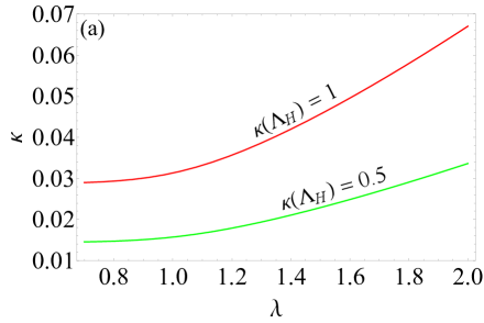
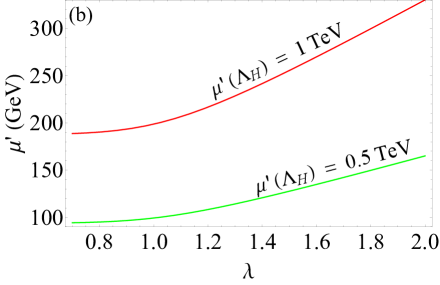
Figure 1: (a): κ𝜅\kappa as a function of λ𝜆\lambda at the scale Q=MZ𝑄subscript𝑀𝑍Q=M_{Z}, obtained by fixing κ𝜅\kappa at the scale ΛHsubscriptΛ𝐻\Lambda_{H} and then evolving it down with RGEs. The red (green) curve corresponds to κ(ΛH)=1(0.5)𝜅subscriptΛ𝐻10.5\kappa(\Lambda_{H})=1(0.5). (b): μsuperscript𝜇\mu^{\prime} as a function of λ𝜆\lambda at the scale Q=MZ𝑄subscript𝑀𝑍Q=M_{Z}, obtained in a manner analogous to (a). The red (green) curve corresponds to μ(ΛH)=1(0.5)TeVsuperscript𝜇subscriptΛ𝐻10.5TeV\mu^{\prime}(\Lambda_{H})=1(0.5)~{}\text{TeV}. In both plots we set tanβ=50𝛽50\tan\beta=50. See text for details of their behavior.

1. Eq. (12) implies κ(ΛH)𝒪(1)much-less-than𝜅subscriptΛ𝐻𝒪1\kappa(\Lambda_{H})\ll\mathcal{O}(1). Run down to a renormalization scale Q=𝒪(TeV)𝑄𝒪TeVQ=\mathcal{O}(\text{TeV}), we expect κ𝜅\kappa to be quickly suppressed due to the contribution of λ𝜆\lambda to its running. This suppression is illustrated in Fig. 1(a), where we plot κ𝜅\kappa at Q=MZ𝑄subscript𝑀𝑍Q=M_{Z} as a function of λ𝜆\lambda at Q=MZ𝑄subscript𝑀𝑍Q=M_{Z}, setting tanβ=50𝛽50\tan\beta=50. These curves were obtained by first running λ(Q=MZ)𝜆𝑄subscript𝑀𝑍\lambda(Q=M_{Z}) up to determine ΛHsubscriptΛ𝐻\Lambda_{H}, then setting κ(Q=ΛH)𝜅𝑄subscriptΛ𝐻\kappa(Q=\Lambda_{H}) to different values 1absent1\leq 1, and finally running κ𝜅\kappa down to Q=MZ𝑄subscript𝑀𝑍Q=M_{Z}. We checked that the running of λ𝜆\lambda is insensitive to κ𝜅\kappa for these sizes of κ𝜅\kappa. The red curve corresponds to κ(ΛH)=1𝜅subscriptΛ𝐻1\kappa(\Lambda_{H})=1 and the green curve to κ(ΛH)=0.5𝜅subscriptΛ𝐻0.5\kappa(\Lambda_{H})=0.5. As expected from the RG running, smaller values of κ(ΛH)𝜅subscriptΛ𝐻\kappa(\Lambda_{H}) result in smaller values of κ(Q=MZ)𝜅𝑄subscript𝑀𝑍\kappa(Q=M_{Z}).

A larger λ𝜆\lambda implies a Landau pole at a lower scale. Therefore, ΛHsubscriptΛ𝐻\Lambda_{H} is closer to the electroweak scale for larger values of λ𝜆\lambda, which in turn weakens the suppression of κ𝜅\kappa as it runs down from ΛHsubscriptΛ𝐻\Lambda_{H} to MZsubscript𝑀𝑍M_{Z}. This is why κ𝜅\kappa is an increasing function of λ𝜆\lambda in Fig. 1(a). From the plot, we infer that for κ(ΛH)1𝜅subscriptΛ𝐻1\kappa(\Lambda_{H})\leq 1, the size of κ𝜅\kappa at the weak scale is suppressed by at least an order of magnitude. The implication of this suppression is that we can consistently neglect the effects of κ𝜅\kappa in our TeV-scale phenomenology. Therefore, for the rest of this paper we will take κ=0𝜅0\kappa=0.

2. As compared to κ𝜅\kappa, μsuperscript𝜇\mu^{\prime} is only suppressed by an 𝒪(1)𝒪1\mathcal{O}(1) number when it is run down from Q=ΛH𝑄subscriptΛ𝐻Q=\Lambda_{H} and Q=MZ𝑄subscript𝑀𝑍Q=M_{Z}. This difference between values of μsuperscript𝜇\mu^{\prime} and κ𝜅\kappa can be understood from their β𝛽\beta-function dependences. Using their one-loop β𝛽\beta-functions in Ref. [43] we find

κ(Q)κ(ΛH)=(μ(Q)μ(ΛH))3.𝜅𝑄𝜅subscriptΛ𝐻superscriptsuperscript𝜇𝑄superscript𝜇subscriptΛ𝐻3\displaystyle\frac{\kappa(Q)}{\kappa(\Lambda_{H})}=\left(\frac{\mu^{\prime}(Q)}{\mu^{\prime}(\Lambda_{H})}\right)^{3}. (14)

We check this by determining μ(Q=MZ)superscript𝜇𝑄subscript𝑀𝑍\mu^{\prime}(Q=M_{Z}) as a function of λ(Q=MZ)𝜆𝑄subscript𝑀𝑍\lambda(Q=M_{Z}) in a manner analogous to the determination of κ(Q=MZ)𝜅𝑄subscript𝑀𝑍\kappa(Q=M_{Z}) above. Our results are shown in Fig. 1(b), where the red (green) curve corresponds to μ(ΛH)=1(0.5)TeVsuperscript𝜇subscriptΛ𝐻10.5TeV\mu^{\prime}(\Lambda_{H})=1(0.5)~{}\text{TeV}, with tanβ=50𝛽50\tan\beta=50. We see that μ(ΛH)superscript𝜇subscriptΛ𝐻\mu^{\prime}(\Lambda_{H}) is suppressed at the electroweak scale by at most a factor of 5. Hence μ(MZ)superscript𝜇subscript𝑀𝑍\mu^{\prime}(M_{Z}) can be of the size of the electoweak scale. Such a size results from reasonable values of the scale Λ0subscriptΛ0\Lambda_{0}. For instance, to obtain μ(Q=MZ)< 1TeVsuperscriptsimilar-tosuperscript𝜇𝑄subscript𝑀𝑍1TeV\mu^{\prime}(Q=M_{Z})\>\raisebox{-2.15277pt}{$\stackrel{{\scriptstyle\textstyle<}}{{\sim}}$}\>1~{}\text{TeV} at tanβ=50𝛽50\tan\beta=50, we computed from Eq. 12 that Λ01016GeVsubscriptΛ0superscript1016GeV\Lambda_{0}\leq 10^{16}~{}\text{GeV} for λ(Q=MZ)0.7𝜆𝑄subscript𝑀𝑍0.7\lambda(Q=M_{Z})\geq 0.7. Similarly, the Higgsino mass parameter μ𝜇\mu and the tadpole term ξF1/2superscriptsubscript𝜉𝐹12\xi_{F}^{1/2} can also be the size of the electroweak scale.

We can now write down our low energy superpotential below the scale ΛHsubscriptΛ𝐻\Lambda_{H}:

𝒲NMSSMeff=𝒲Yukawa+λS^H^uH^d+12μS^2+ξFS^superscriptsubscript𝒲NMSSMeffsubscript𝒲Yukawa𝜆^𝑆subscript^𝐻𝑢subscript^𝐻𝑑12superscript𝜇superscript^𝑆2subscript𝜉𝐹^𝑆\displaystyle\mathcal{W}_{\rm NMSSM}^{\rm eff}=\mathcal{W}_{\rm Yukawa}+\lambda\hat{S}\hat{H}_{u}\hat{H}_{d}+\frac{1}{2}\mu^{\prime}\hat{S}^{2}+\xi_{F}\hat{S} (15)

The associated soft-SUSY breaking potential is

softeffsuperscriptsubscriptsofteff\displaystyle-\mathcal{L}_{\rm soft}^{\rm eff} =\displaystyle= softf~+mHu2|Hu|2+mHd2|Hd|2+mS2|S|2superscriptsubscriptsoft~𝑓superscriptsubscript𝑚subscript𝐻𝑢2superscriptsubscript𝐻𝑢2superscriptsubscript𝑚subscript𝐻𝑑2superscriptsubscript𝐻𝑑2superscriptsubscript𝑚𝑆2superscript𝑆2\displaystyle-\mathcal{L}_{\rm soft}^{\tilde{f}}+m_{H_{u}}^{2}|H_{u}|^{2}+m_{H_{d}}^{2}|H_{d}|^{2}+m_{S}^{2}|S|^{2} (16)
+(λAλSHuHd+m32HuHd+12mS2+ξSS+h.c.).\displaystyle+\left(\lambda A_{\lambda}SH_{u}H_{d}+m_{3}^{2}H_{u}H_{d}+\frac{1}{2}m^{\prime 2}_{S}+\xi_{S}S+{\rm h.c.}\right).

We have redefined the singlet chiral superfield, S^S^μ^𝑆^𝑆𝜇\hat{S}\to\hat{S}-\mu, to remove the μ𝜇\mu term in the superpotential. In general, the associated soft term m32superscriptsubscript𝑚32m_{3}^{2} cannot be absorbed into Aλsubscript𝐴𝜆A_{\lambda} simultaneously. Eqs. (15) and Eq. (16) constitute all the parameters treated in the rest of this article.

2.2 Higgs Sector

2.2.1 Tree level

At the tree level, the Higgs potential is given by

VHiggstree=VF+VD+VSsuperscriptsubscript𝑉Higgstreesubscript𝑉𝐹subscript𝑉𝐷subscript𝑉𝑆\displaystyle V_{\rm Higgs}^{\rm tree}=V_{F}+V_{D}+V_{S} (17)

where

VFsubscript𝑉𝐹\displaystyle V_{F} =\displaystyle= |λ(Hu+HdHu0Hd0)+μS+ξF|2+|λS|2(|Hu|2+|Hd|2),superscript𝜆superscriptsubscript𝐻𝑢superscriptsubscript𝐻𝑑superscriptsubscript𝐻𝑢0superscriptsubscript𝐻𝑑0superscript𝜇𝑆subscript𝜉𝐹2superscript𝜆𝑆2superscriptsubscript𝐻𝑢2superscriptsubscript𝐻𝑑2\displaystyle\left|\lambda\left(H_{u}^{+}H_{d}^{-}-H_{u}^{0}H_{d}^{0}\right)+\mu^{\prime}S+\xi_{F}\right|^{2}+\left|\lambda S\right|^{2}\ (\left|H_{u}\right|^{2}+\left|H_{d}\right|^{2}),
VDsubscript𝑉𝐷\displaystyle V_{D} =\displaystyle= g28(|Hu0|2+|Hu+|2|Hd0|2|Hd|2)+g22cos2θW|Hu+Hd0+Hu0Hd|2,superscript𝑔28superscriptsuperscriptsubscript𝐻𝑢02superscriptsuperscriptsubscript𝐻𝑢2superscriptsuperscriptsubscript𝐻𝑑02superscriptsuperscriptsubscript𝐻𝑑2superscript𝑔22superscript2subscript𝜃𝑊superscriptsuperscriptsubscript𝐻𝑢superscriptsubscript𝐻𝑑0superscriptsubscript𝐻𝑢0superscriptsubscript𝐻𝑑absent2\displaystyle\frac{g^{2}}{8}\left(\left|H_{u}^{0}\right|^{2}+\left|H_{u}^{+}\right|^{2}-\left|H_{d}^{0}\right|^{2}-\left|H_{d}^{-}\right|^{2}\right)+\frac{g^{2}}{2}\cos^{2}\theta_{W}\left|H_{u}^{+}H_{d}^{0*}+H_{u}^{0}H_{d}^{-*}\right|^{2}, (18)
VSsubscript𝑉𝑆\displaystyle V_{S} =\displaystyle= mHu2|Hu|2+mHd2|Hd|2+mS2|S|2+superscriptsubscript𝑚subscript𝐻𝑢2superscriptsubscript𝐻𝑢2superscriptsubscript𝑚subscript𝐻𝑑2superscriptsubscript𝐻𝑑2limit-fromsuperscriptsubscript𝑚𝑆2superscript𝑆2\displaystyle m_{H_{u}}^{2}|H_{u}|^{2}+m_{H_{d}}^{2}|H_{d}|^{2}+m_{S}^{2}|S|^{2}+
(λAλ(Hu+HdHu0Hd0)S+m32(Hu+HdHu0Hd0)+12mS2S2+ξSS+h.c.),\displaystyle(\lambda A_{\lambda}(H_{u}^{+}H_{d}^{-}-H_{u}^{0}H_{d}^{0})S+m_{3}^{2}(H_{u}^{+}H_{d}^{-}-H_{u}^{0}H_{d}^{0})+\frac{1}{2}m^{{}^{\prime}2}_{S}S^{2}+\xi_{S}S+{\rm h.c.}),

Hu=(Hu+,Hu0)subscript𝐻𝑢superscriptsubscript𝐻𝑢superscriptsubscript𝐻𝑢0H_{u}=(H_{u}^{+},H_{u}^{0}), Hd=(Hd0,Hd),g2g12+g22formulae-sequencesubscript𝐻𝑑superscriptsubscript𝐻𝑑0superscriptsubscript𝐻𝑑superscript𝑔2subscriptsuperscript𝑔21subscriptsuperscript𝑔22H_{d}=(H_{d}^{0},H_{d}^{-}),~{}g^{2}\equiv g^{2}_{1}+g^{2}_{2} and θWsubscript𝜃𝑊\theta_{W} is the weak mixing angle. After electroweak symmetry breaking we can expand the Higgs fields in terms of the CP-even fields (hu0,hd0,hs0)superscriptsubscript𝑢0superscriptsubscript𝑑0superscriptsubscript𝑠0(h_{u}^{0},h_{d}^{0},h_{s}^{0}), the CP-odd fields (AD0,AS0)superscriptsubscript𝐴𝐷0superscriptsubscript𝐴𝑆0(A_{D}^{0},A_{S}^{0}), the charged Higgs bosons H±superscript𝐻plus-or-minusH^{\pm} and the Goldstone bosons (G±,G0)superscript𝐺plus-or-minussuperscript𝐺0(G^{\pm},G^{0}):

Husubscript𝐻𝑢\displaystyle H_{u} =\displaystyle= (G+sβ+H+cβvsβ+12[(hu0+i(G0sβAD0cβ)]),\displaystyle\left(\begin{array}[]{c}G^{+}s_{\beta}+H^{+}c_{\beta}\\ vs_{\beta}+\frac{1}{\sqrt{2}}[(h_{u}^{0}+i(G^{0}s_{\beta}-A_{D}^{0}c_{\beta})]\end{array}\right), (21)
Hdsubscript𝐻𝑑\displaystyle H_{d} =\displaystyle= (vcβ+12[(hd0+i(G0cβ+AD0sβ)]Gcβ+Hsβ),\displaystyle\left(\begin{array}[]{c}vc_{\beta}+\frac{1}{\sqrt{2}}[(h_{d}^{0}+i(-G^{0}c_{\beta}+A_{D}^{0}s_{\beta})]\\ -G^{-}c_{\beta}+H^{-}s_{\beta}\end{array}\right), (24)
S𝑆\displaystyle S =\displaystyle= 12(s+hs0+iAS0),12𝑠subscriptsuperscript0𝑠𝑖subscriptsuperscript𝐴0𝑆\displaystyle\frac{1}{\sqrt{2}}(s+h^{0}_{s}+iA^{0}_{S}), (25)

where v174GeVsimilar-to-or-equals𝑣174GeVv\simeq 174~{}\text{GeV} is the VEV of EWSB, sβsinβ,cβcosβformulae-sequencesubscript𝑠𝛽𝛽subscript𝑐𝛽𝛽s_{\beta}\equiv\sin\beta,~{}c_{\beta}\equiv\cos\beta and sS𝑠delimited-⟨⟩𝑆s\equiv\langle S\rangle. Expanding the potential about the minimum at vi(vu,vd,s)subscript𝑣𝑖subscript𝑣𝑢subscript𝑣𝑑𝑠v_{i}\equiv(v_{u},v_{d},s), we can find the tree-level tadpole terms

TjtreeVHiggstreeϕj|{vi}superscriptsubscript𝑇𝑗treeevaluated-atsuperscriptsubscript𝑉Higgstreesubscriptitalic-ϕ𝑗subscript𝑣𝑖\displaystyle T_{j}^{\rm tree}\equiv\left.\frac{\partial V_{\rm Higgs}^{\rm tree}}{\partial\phi_{j}}\right|_{\{v_{i}\}} (26)

where ϕj=(Hu0,Hd0,S)subscriptitalic-ϕ𝑗superscriptsubscript𝐻𝑢0superscriptsubscript𝐻𝑑0𝑆\phi_{j}=(H_{u}^{0},H_{d}^{0},S). We can then solve for the soft squared masses mHu2,mHd2,mS2superscriptsubscript𝑚subscript𝐻𝑢2superscriptsubscript𝑚subscript𝐻𝑑2superscriptsubscript𝑚𝑆2m_{H_{u}}^{2},m_{H_{d}}^{2},m_{S}^{2} by setting each Tjtree=0superscriptsubscript𝑇𝑗tree0T_{j}^{\rm tree}=0. Substituting these masses into the second order derivatives of the Higgs potential and neglecting CP-violating effects, we obtain the following tree-level CP-even Higgs mass matrix in the basis (hu0,hd0,hs0)subscriptsuperscript0𝑢subscriptsuperscript0𝑑subscriptsuperscript0𝑠(h^{0}_{u},h^{0}_{d},h^{0}_{s}).

(MH2)11=MZ2sβ2+rtβ1;subscriptsubscriptsuperscript𝑀2𝐻11subscriptsuperscript𝑀2𝑍subscriptsuperscript𝑠2𝛽𝑟subscriptsuperscript𝑡1𝛽\displaystyle\left(M^{2}_{H}\right)_{11}=M^{2}_{Z}s^{2}_{\beta}+r~{}t^{-1}_{\beta}; (MH2)12=(2λ2v2MZ2)sβcβr;subscriptsubscriptsuperscript𝑀2𝐻122superscript𝜆2superscript𝑣2subscriptsuperscript𝑀2𝑍subscript𝑠𝛽subscript𝑐𝛽𝑟\displaystyle\left(M^{2}_{H}\right)_{12}=(2\lambda^{2}v^{2}-M^{2}_{Z})s_{\beta}c_{\beta}-r;
(MH2)22=MZ2cβ2+rtβ;subscriptsubscriptsuperscript𝑀2𝐻22subscriptsuperscript𝑀2𝑍subscriptsuperscript𝑐2𝛽𝑟subscript𝑡𝛽\displaystyle\left(M^{2}_{H}\right)_{22}=M^{2}_{Z}c^{2}_{\beta}+r~{}t_{\beta}; (MH2)13=λv(2μeffsβ(Aλ+μ)cβ);subscriptsubscriptsuperscript𝑀2𝐻13𝜆𝑣2subscript𝜇effsubscript𝑠𝛽subscript𝐴𝜆superscript𝜇subscript𝑐𝛽\displaystyle\left(M^{2}_{H}\right)_{13}=\lambda v(2\mu_{\text{eff}}s_{\beta}-(A_{\lambda}+\mu^{\prime})c_{\beta}); (27)
(MH2)23=λv(2μeffcβ(Aλ+μ)sβ);subscriptsubscriptsuperscript𝑀2𝐻23𝜆𝑣2subscript𝜇effsubscript𝑐𝛽subscript𝐴𝜆superscript𝜇subscript𝑠𝛽\displaystyle\left(M^{2}_{H}\right)_{23}=\lambda v(2\mu_{\text{eff}}c_{\beta}-(A_{\lambda}+\mu^{\prime})s_{\beta}); (MH2)33=(λv2(Aλ+μ)(ξS+ξFμ))/s,subscriptsubscriptsuperscript𝑀2𝐻33𝜆superscript𝑣2subscript𝐴𝜆superscript𝜇subscript𝜉𝑆subscript𝜉𝐹superscript𝜇𝑠\displaystyle\left(M^{2}_{H}\right)_{33}=\left(\lambda v^{2}(A_{\lambda}+\mu^{\prime})-(\xi_{S}+\xi_{F}\mu^{\prime})\right)/s,

where μeffλs,tβtanβformulae-sequencesubscript𝜇eff𝜆𝑠subscript𝑡𝛽𝛽\mu_{\text{eff}}\equiv\lambda s,~{}t_{\beta}\equiv\tan\beta and rμeff(Aλ+μ)+m32+λξF𝑟subscript𝜇effsubscript𝐴𝜆superscript𝜇subscriptsuperscript𝑚23𝜆subscript𝜉𝐹r\equiv\mu_{\text{eff}}(A_{\lambda}+\mu^{\prime})+m^{2}_{3}+\lambda\xi_{F}. The CP-odd Higgs mass matrix in the basis (AD0,AS0)superscriptsubscript𝐴𝐷0superscriptsubscript𝐴𝑆0(A_{D}^{0},A_{S}^{0}) is given by

(MA2)11=2r/s2β;(MA2)12=λv(Aλμ);formulae-sequencesubscriptsubscriptsuperscript𝑀2𝐴112𝑟subscript𝑠2𝛽subscriptsubscriptsuperscript𝑀2𝐴12𝜆𝑣subscript𝐴𝜆superscript𝜇\displaystyle\left(M^{2}_{A}\right)_{11}=2r/s_{2\beta};\;\;\;\;\;\;\left(M^{2}_{A}\right)_{12}=\lambda v(A_{\lambda}-\mu^{\prime});
(MA2)22=1s(λv2(Aλ+μ)sβcβ(ξFμ+ξS))2mS2,subscriptsubscriptsuperscript𝑀2𝐴221𝑠𝜆superscript𝑣2subscript𝐴𝜆superscript𝜇subscript𝑠𝛽subscript𝑐𝛽subscript𝜉𝐹superscript𝜇subscript𝜉𝑆2superscriptsubscriptsuperscript𝑚𝑆2\displaystyle\left(M^{2}_{A}\right)_{22}=\frac{1}{s}\left(\lambda v^{2}(A_{\lambda}+\mu^{\prime})s_{\beta}c_{\beta}-(\xi_{F}\mu^{\prime}+\xi_{S})\right)-2{m^{\prime}}_{S}^{2}, (28)

and the charged Higgs mass is

M±2=2r/s2β(λ2g22/2)v2.subscriptsuperscript𝑀2plus-or-minus2𝑟subscript𝑠2𝛽superscript𝜆2subscriptsuperscript𝑔222superscript𝑣2\displaystyle M^{2}_{\pm}=2r/s_{2\beta}-(\lambda^{2}-g^{2}_{2}/2)v^{2}. (29)

We point out two features of the tree level masses that will be important in our discussion of the one-loop corrected Higgs mass. The first feature is the correlation among the scalar masses in the limit where Aλsubscript𝐴𝜆A_{\lambda} and μsuperscript𝜇\mu^{\prime} are small compared to the heavy Higgs masses. This is best seen by setting (MA2)12=0subscriptsubscriptsuperscript𝑀2𝐴120\left(M^{2}_{A}\right)_{12}=0 in Eq. (28) (which can be obtained by choosing Aλ=μsubscript𝐴𝜆superscript𝜇A_{\lambda}=\mu^{\prime}). Then the CP-odd eigenmasses are identified as MAD2=(MA2)11subscriptsuperscript𝑀2subscript𝐴𝐷subscriptsubscriptsuperscript𝑀2𝐴11M^{2}_{A_{D}}=\left(M^{2}_{A}\right)_{11} and MAS2=(MA2)22subscriptsuperscript𝑀2subscript𝐴𝑆subscriptsubscriptsuperscript𝑀2𝐴22M^{2}_{A_{S}}=\left(M^{2}_{A}\right)_{22}. In this limit, by inspecting the matrix elements in Eqs. (27)–(29), we find that the CP-even, CP-odd and charged Higgs eigenstates arising from the SU(2)𝑆𝑈2SU(2) doublet sector are nearly degenerate in mass, a feature well-known in the MSSM. Their mass splittings v2similar-toabsentsuperscript𝑣2\sim v^{2}. These three fields then have a mass MADsimilar-toabsentsubscript𝑀subscript𝐴𝐷\sim M_{A_{D}} in the limit MAD2v2,Aλ2,μ2much-greater-thansubscriptsuperscript𝑀2subscript𝐴𝐷superscript𝑣2superscriptsubscript𝐴𝜆2superscript𝜇2M^{2}_{A_{D}}\gg v^{2},A_{\lambda}^{2},\mu^{\prime 2}, where MADsubscript𝑀subscript𝐴𝐷M_{A_{D}} denotes the corresponding CP-odd eigenmass. Likewise, the CP-even and CP-odd Higgs eigenstates arising from the SU(2)𝑆𝑈2SU(2) singlet are nearly degenerate, with mass splitting s2similar-toabsentsuperscript𝑠2\sim s^{2}. Therefore, these two fields have a mass MASsimilar-toabsentsubscript𝑀subscript𝐴𝑆\sim M_{A_{S}} in the limit MAS2s2,Aλ2,μ2much-greater-thansubscriptsuperscript𝑀2subscript𝐴𝑆superscript𝑠2superscriptsubscript𝐴𝜆2superscript𝜇2M^{2}_{A_{S}}\gg s^{2},A_{\lambda}^{2},\mu^{\prime 2}.

The second feature is the decoupling of heavy states. Raising MAD2subscriptsuperscript𝑀2subscript𝐴𝐷M^{2}_{A_{D}} and MAS2subscriptsuperscript𝑀2subscript𝐴𝑆M^{2}_{A_{S}} decreases their impact on the mass of the lightest CP-even state, effectively making it more SM-like. A simple way to see this decoupling behavior is to rotate the CP-even mass matrix into the basis

h0=hu0sβ+hd0cβ,H0=hu0cβhd0sβ,hs0=hs0formulae-sequencesuperscript0superscriptsubscript𝑢0subscript𝑠𝛽superscriptsubscript𝑑0subscript𝑐𝛽formulae-sequencesuperscript𝐻0superscriptsubscript𝑢0subscript𝑐𝛽superscriptsubscript𝑑0subscript𝑠𝛽subscriptsuperscript0𝑠subscriptsuperscript0𝑠\displaystyle h^{0}=h_{u}^{0}s_{\beta}+h_{d}^{0}c_{\beta},~{}H^{0}=h_{u}^{0}c_{\beta}-h_{d}^{0}s_{\beta},~{}h^{0}_{s}=h^{0}_{s} (30)

which leads to the CP-even mass matrix

(MH2)hh=MZ2c2β2+λ2v2s2β2;subscriptsubscriptsuperscript𝑀2𝐻subscriptsuperscript𝑀2𝑍subscriptsuperscript𝑐22𝛽superscript𝜆2superscript𝑣2subscriptsuperscript𝑠22𝛽\displaystyle\left(M^{2}_{H}\right)_{hh}=M^{2}_{Z}c^{2}_{2\beta}+\lambda^{2}v^{2}s^{2}_{2\beta}; (MH2)hH=(λ2v2MZ2)s4β/2;subscriptsubscriptsuperscript𝑀2𝐻𝐻superscript𝜆2superscript𝑣2superscriptsubscript𝑀𝑍2subscript𝑠4𝛽2\displaystyle\left(M^{2}_{H}\right)_{hH}=(\lambda^{2}v^{2}-M_{Z}^{2})s_{4\beta}/2;
(MH2)HH=MAD2(λ2v2MZ2)s2β2;subscriptsubscriptsuperscript𝑀2𝐻𝐻𝐻subscriptsuperscript𝑀2subscript𝐴𝐷superscript𝜆2superscript𝑣2superscriptsubscript𝑀𝑍2subscriptsuperscript𝑠22𝛽\displaystyle\left(M^{2}_{H}\right)_{HH}=M^{2}_{A_{D}}-(\lambda^{2}v^{2}-M_{Z}^{2})s^{2}_{2\beta}; (MH2)hS=2λv(μeffAλs2β);subscriptsubscriptsuperscript𝑀2𝐻𝑆2𝜆𝑣subscript𝜇effsubscript𝐴𝜆subscript𝑠2𝛽\displaystyle\left(M^{2}_{H}\right)_{hS}=2\lambda v(\mu_{\text{eff}}-A_{\lambda}s_{2\beta}); (31)
(MH2)HS=2λvAλc2β;subscriptsubscriptsuperscript𝑀2𝐻𝐻𝑆2𝜆𝑣subscript𝐴𝜆subscript𝑐2𝛽\displaystyle\left(M^{2}_{H}\right)_{HS}=-2\lambda vA_{\lambda}c_{2\beta}; (MH2)SS=MAS2+2mS2+λ2v2μeffAλ(2s2βcβ),subscriptsubscriptsuperscript𝑀2𝐻𝑆𝑆subscriptsuperscript𝑀2subscript𝐴𝑆2superscriptsubscriptsuperscript𝑚𝑆2superscript𝜆2superscript𝑣2subscript𝜇effsubscript𝐴𝜆2subscript𝑠2𝛽subscript𝑐𝛽\displaystyle\left(M^{2}_{H}\right)_{SS}=M^{2}_{A_{S}}+2{m^{\prime}_{S}}^{2}+{\lambda^{2}v^{2}\over\mu_{\text{eff}}}A_{\lambda}(2-s_{2\beta}c_{\beta}),

Notice that ξF,ξSsubscript𝜉𝐹subscript𝜉𝑆\xi_{F},\xi_{S} and m32subscriptsuperscript𝑚23m^{2}_{3} are absorbed into our definition of MAD2subscriptsuperscript𝑀2subscript𝐴𝐷M^{2}_{A_{D}} and MAS2subscriptsuperscript𝑀2subscript𝐴𝑆M^{2}_{A_{S}}. For large tanβ𝛽\tan\beta, MAD2subscriptsuperscript𝑀2subscript𝐴𝐷M^{2}_{A_{D}} and MAS2subscriptsuperscript𝑀2subscript𝐴𝑆M^{2}_{A_{S}}, h0superscript0h^{0} is identified with the SM Higgs, and H0superscript𝐻0H^{0} and hs0subscriptsuperscript0𝑠h^{0}_{s} with non-standard Higgs bosons. This decoupling feature should be preserved after the inclusion of radiative corrections to the lightest CP-even Higgs mass, which is a non-trivial check of this computation.

2.2.2 Radiative corrections

The mass of the lightest Higgs boson can be significantly modified by one-loop corrections. The largest contributions to the Higgs potential at one-loop level are from the Higgs bosons, third generation squarks, charginos and neutralinos. Thus we have

ΔVΔ𝑉\displaystyle\Delta V =\displaystyle= 132π2(3ΔVt~6ΔVtΔVχ±2ΔVχ0+12ΔVH+12ΔVA+ΔVH±),132superscript𝜋23Δsuperscript𝑉~𝑡6Δsuperscript𝑉𝑡Δsuperscript𝑉superscript𝜒plus-or-minus2Δsuperscript𝑉superscript𝜒012Δsuperscript𝑉𝐻12Δsuperscript𝑉𝐴Δsuperscript𝑉superscript𝐻plus-or-minus\displaystyle\frac{1}{32\pi^{2}}\left(3\Delta V^{\tilde{t}}-6\Delta V^{t}-\Delta V^{\chi^{\pm}}-2\Delta V^{\chi^{0}}+\frac{1}{2}\Delta V^{H}+\frac{1}{2}\Delta V^{A}+\Delta V^{H^{\pm}}\right), (32)

where for the athsuperscript𝑎tha^{\rm th} sector in the MS¯¯MS\overline{\text{MS}} scheme,

ΔVa=i(Mia2(ϕk))2(logMia2(ϕk)Q232)i=heavy(Mia2(ϕk))2(logMia2Q232).Δsuperscript𝑉𝑎subscript𝑖superscriptsuperscriptsubscript𝑀𝑖𝑎2subscriptitalic-ϕ𝑘2superscriptsubscript𝑀𝑖𝑎2subscriptitalic-ϕ𝑘superscript𝑄232subscript𝑖heavysuperscriptsuperscriptsubscript𝑀𝑖𝑎2subscriptitalic-ϕ𝑘2superscriptsubscript𝑀𝑖𝑎2superscript𝑄232\displaystyle\Delta V^{a}=\sum_{i}\left(M_{ia}^{2}(\phi_{k})\right)^{2}\left(\log\frac{M_{ia}^{2}(\phi_{k})}{Q^{2}}-\frac{3}{2}\right)\approx\sum_{i=\rm heavy}\left(M_{ia}^{2}(\phi_{k})\right)^{2}\left(\log\frac{M_{ia}^{2}}{Q^{2}}-\frac{3}{2}\right). (33)

Mia2(ϕk)superscriptsubscript𝑀𝑖𝑎2subscriptitalic-ϕ𝑘M_{ia}^{2}(\phi_{k}) is the field-dependent mass eigenvalue for ithsuperscript𝑖thi^{\rm th} contribution, Mia2superscriptsubscript𝑀𝑖𝑎2M_{ia}^{2} is the corresponding field-independent tree-level eigenvalue and the renormalization scale Qmh=125similar-to𝑄subscript𝑚125Q\sim m_{h}=125 GeV. The approximation in Eq. (33) holds because we are interested in large corrections to the lightest Higgs mass due to states much heavier than the electroweak scale. Also, the field dependences inside log\log terms are neglected since they only induce higher order field-dependent terms.

The dominant contributions to ΔVΔ𝑉\Delta V in our scenario are due to heavy Higgs scalars coupling to the light Higgs boson with strengths proportional to powers of λ𝜆\lambda. The effects of the top quarks and the scalar tops on the Higgs potential have been studied in great detail in Refs. [4, 5, 6, 7, 8, 9, 10, 11, 12, 13, 14]. To highlight the effect of large λ𝜆\lambda corrections, we suppress the contribution of scalar tops to ΔVΔ𝑉\Delta V by choosing their masses close to the electroweak scale while still being compatible with ATLAS and CMS bounds [47, 48, 49]. The contributions of charginos and neutralinos to ΔVΔ𝑉\Delta V are typically small. The Higgs couples to the bino and the wino triplet with electroweak strength, whereas the λ𝜆\lambda-dependent coupling to the Higgsinos and singlino is typically suppressed due to neutralino mixing. In addition, the masses of the Higgsinos and singlino  <superscriptsimilar-to\stackrel{{\scriptstyle\textstyle<}}{{\sim}}  1 TeV in our phenomenology while MA[4,8]TeVsubscript𝑀𝐴48TeVM_{A}\in[4,8]~{}\text{TeV}. We therefore neglect corrections from the chargino-neutralino sector in the remainder of this article.

In order to compute the one-loop corrections to the Higgs potential in Eq. (33) due to the heavy CP-even, CP-odd and charged Higgs bosons, we must determine the field-dependent eigenvalues of each of the respective matrices. When expressed in terms of the matrix elements these field-dependent eigenvalues can in general be quite complicated. The calculation can nevertheless be simplified if we expand the eigenvalues as a Taylor series in the tree-level masses:

Mi2(ϕk)=Mi,tree2+b^i(ϕk)+c^i(ϕk)Mi,tree2+𝒪(1Mi,tree4),subscriptsuperscript𝑀2𝑖subscriptitalic-ϕ𝑘subscriptsuperscript𝑀2𝑖treesubscript^𝑏𝑖subscriptitalic-ϕ𝑘subscript^𝑐𝑖subscriptitalic-ϕ𝑘subscriptsuperscript𝑀2𝑖tree𝒪1subscriptsuperscript𝑀4𝑖treeM^{2}_{i}(\phi_{k})=M^{2}_{i,{\rm tree}}+\hat{b}_{i}(\phi_{k})+\frac{\hat{c}_{i}(\phi_{k})}{M^{2}_{i,{\rm tree}}}+\mathcal{O}\left(\frac{1}{M^{4}_{i,{\rm tree}}}\right), (34)

where the coefficients b^i(ϕk)subscript^𝑏𝑖subscriptitalic-ϕ𝑘\hat{b}_{i}(\phi_{k}) and c^i(ϕk)subscript^𝑐𝑖subscriptitalic-ϕ𝑘\hat{c}_{i}(\phi_{k}) are at most quadratic and quartic in the fields respectively. Furthermore, when evaluated at the tree-level VEVs, the coefficients satisfy the condition b^({vk})=0=c^({vk})^𝑏subscript𝑣𝑘0^𝑐subscript𝑣𝑘\hat{b}(\{v_{k}\})=0=\hat{c}(\{v_{k}\}).

In practice, we expand the eigenvalues as a Taylor series in the pseudoscalar masses MAD2subscriptsuperscript𝑀2subscript𝐴𝐷M^{2}_{A_{D}} and MAS2subscriptsuperscript𝑀2subscript𝐴𝑆M^{2}_{A_{S}}. Using these approximations the one-loop effective potential due to the heavy Higgs scalars now evaluates to

ΔVi[aiMA,i4+2biMA,i2+(bi2+2ci)](logMA,i2Q232)proportional-toΔ𝑉subscript𝑖delimited-[]subscript𝑎𝑖subscriptsuperscript𝑀4𝐴𝑖2subscript𝑏𝑖subscriptsuperscript𝑀2𝐴𝑖superscriptsubscript𝑏𝑖22subscript𝑐𝑖subscriptsuperscript𝑀2𝐴𝑖superscript𝑄232\displaystyle\Delta V\propto\sum_{i}\left[a_{i}M^{4}_{A,i}+2b_{i}M^{2}_{A,i}+(b_{i}^{2}+2c_{i})\right]\left(\log\frac{M^{2}_{A,i}}{Q^{2}}-\frac{3}{2}\right) (35)

where aisubscript𝑎𝑖a_{i} are constants and the field-dependent coefficients bisubscript𝑏𝑖b_{i} and cisubscript𝑐𝑖c_{i} are obtained from the hatted coefficients in Eq. (34). Reducing ΔVΔ𝑉\Delta V to this form considerably simplifies the calculation of Higgs mass corrections. ΔVΔ𝑉\Delta V as presented here must also ensure that the decoupling behavior discussed in the previous subsection is preserved at one-loop order. This result is demonstrated in Appendix A.

The full details of our computation and the corresponding results are presented in Appendix B, where two cases satisfying the condition (MA2)12=0subscriptsubscriptsuperscript𝑀2𝐴120\left(M^{2}_{A}\right)_{12}=0 in Eq. (28) were considered. In the first case, which we call Case (A), we assume that the one-loop corrections arise from a single heavy scale MA=MAD=MASsubscript𝑀𝐴subscript𝑀subscript𝐴𝐷subscript𝑀subscript𝐴𝑆M_{A}=M_{A_{D}}=M_{A_{S}}. The results from this case will be used in our discussion of phenomenology in Section 3. In the second case, which we call Case (B), we show the effect of splitting the CP-odd Higgs masses, thereby obtaining corrections from two heavy scales. In this case we set the terms Aλ,μ,Aκ,m3,mSsubscript𝐴𝜆superscript𝜇subscript𝐴𝜅subscript𝑚3subscriptsuperscript𝑚𝑆A_{\lambda},\mu^{\prime},A_{\kappa},m_{3},m^{\prime}_{S} to zero for simplicity. Further, we ignored corrections that depend on electroweak couplings since we are interested in the limit λgmuch-greater-than𝜆𝑔\lambda\gg g. It is important to note that Cases (A) and (B) pertain not only to different limits of the mass spectra of the CP-odd scalars, but also to somewhat different regions of the Lagrangian parameters. In Case (A), the parameters Aλ,μ,Aκ,m3,mSsubscript𝐴𝜆superscript𝜇subscript𝐴𝜅subscript𝑚3subscriptsuperscript𝑚𝑆A_{\lambda},\mu^{\prime},A_{\kappa},m_{3},m^{\prime}_{S} can be non-zero in general, with the condition (MA2)12=0subscriptsubscriptsuperscript𝑀2𝐴120\left(M^{2}_{A}\right)_{12}=0 imposing Aλ=μsubscript𝐴𝜆superscript𝜇A_{\lambda}=\mu^{\prime}. On the other hand, Case (B) explicitly sets them all to zero.

For Case B, the one-loop self-energy corrections obtained in the basis (hu0,hd0,hs0subscriptsuperscript0𝑢subscriptsuperscript0𝑑subscriptsuperscript0𝑠h^{0}_{u},h^{0}_{d},h^{0}_{s}) are

Π11subscriptΠ11\displaystyle\Pi_{11} =\displaystyle= λ4v216π2sβ2[(4c2β+c4β+1)log(MAD2MZ2)+2log(MAS2MZ2)],superscript𝜆4superscript𝑣216superscript𝜋2subscriptsuperscript𝑠2𝛽delimited-[]4subscript𝑐2𝛽subscript𝑐4𝛽1subscriptsuperscript𝑀2subscript𝐴𝐷subscriptsuperscript𝑀2𝑍2subscriptsuperscript𝑀2subscript𝐴𝑆subscriptsuperscript𝑀2𝑍\displaystyle\frac{\lambda^{4}v^{2}}{16\pi^{2}}s^{2}_{\beta}\left[-(4c_{2\beta}+c_{4\beta}+1)\log\left(\frac{M^{2}_{A_{D}}}{M^{2}_{Z}}\right)+2\log\left(\frac{M^{2}_{A_{S}}}{M^{2}_{Z}}\right)\right],
Π12subscriptΠ12\displaystyle\Pi_{12} =\displaystyle= 2λ4v216π2sβcβ(2+c4β)log(MAD2MZ2),2superscript𝜆4superscript𝑣216superscript𝜋2subscript𝑠𝛽subscript𝑐𝛽2subscript𝑐4𝛽subscriptsuperscript𝑀2subscript𝐴𝐷subscriptsuperscript𝑀2𝑍\displaystyle\frac{2\lambda^{4}v^{2}}{16\pi^{2}}s_{\beta}c_{\beta}(2+c_{4\beta})\log\left(\frac{M^{2}_{A_{D}}}{M^{2}_{Z}}\right),
Π22subscriptΠ22\displaystyle\Pi_{22} =\displaystyle= λ4v216π2cβ2[(4c2β+c4β+1)log(MAD2MZ2)+2log(MAS2MZ2)],superscript𝜆4superscript𝑣216superscript𝜋2subscriptsuperscript𝑐2𝛽delimited-[]4subscript𝑐2𝛽subscript𝑐4𝛽1subscriptsuperscript𝑀2subscript𝐴𝐷subscriptsuperscript𝑀2𝑍2subscriptsuperscript𝑀2subscript𝐴𝑆subscriptsuperscript𝑀2𝑍\displaystyle\frac{\lambda^{4}v^{2}}{16\pi^{2}}c^{2}_{\beta}\left[-(-4c_{2\beta}+c_{4\beta}+1)\log\left(\frac{M^{2}_{A_{D}}}{M^{2}_{Z}}\right)+2\log\left(\frac{M^{2}_{A_{S}}}{M^{2}_{Z}}\right)\right],
Π13subscriptΠ13\displaystyle\Pi_{13} =\displaystyle= λ3vμeff16π2sβ[(1+3c2β)log(MAD2MZ2)+4log(MAS2MZ2)],superscript𝜆3𝑣subscript𝜇eff16superscript𝜋2subscript𝑠𝛽delimited-[]13subscript𝑐2𝛽subscriptsuperscript𝑀2subscript𝐴𝐷subscriptsuperscript𝑀2𝑍4subscriptsuperscript𝑀2subscript𝐴𝑆subscriptsuperscript𝑀2𝑍\displaystyle\frac{\lambda^{3}v\mu_{\text{eff}}}{16\pi^{2}}s_{\beta}\left[-(1+3c_{2\beta})\log\left(\frac{M^{2}_{A_{D}}}{M^{2}_{Z}}\right)+4\log\left(\frac{M^{2}_{A_{S}}}{M^{2}_{Z}}\right)\right],
Π23subscriptΠ23\displaystyle\Pi_{23} =\displaystyle= λ3vμeff16π2cβ[(13c2β)log(MAD2MZ2)+4log(MAS2MZ2)],superscript𝜆3𝑣subscript𝜇eff16superscript𝜋2subscript𝑐𝛽delimited-[]13subscript𝑐2𝛽subscriptsuperscript𝑀2subscript𝐴𝐷subscriptsuperscript𝑀2𝑍4subscriptsuperscript𝑀2subscript𝐴𝑆subscriptsuperscript𝑀2𝑍\displaystyle\frac{\lambda^{3}v\mu_{\text{eff}}}{16\pi^{2}}c_{\beta}\left[-(1-3c_{2\beta})\log\left(\frac{M^{2}_{A_{D}}}{M^{2}_{Z}}\right)+4\log\left(\frac{M^{2}_{A_{S}}}{M^{2}_{Z}}\right)\right],
Π33subscriptΠ33\displaystyle\Pi_{33} =\displaystyle= 4λ2μeff216π2log(MAD2MZ2).4superscript𝜆2superscriptsubscript𝜇eff216superscript𝜋2subscriptsuperscript𝑀2subscript𝐴𝐷subscriptsuperscript𝑀2𝑍\displaystyle\frac{4\lambda^{2}\mu_{\text{eff}}^{2}}{16\pi^{2}}\log\left(\frac{M^{2}_{A_{D}}}{M^{2}_{Z}}\right).

When these contributions are rotated into the basis of Eq. (30), we get the (1, 1) element of the self-energy corrections as

Πhh=λ4v2sβ16π2[(cβ2(2+c4β)sβ2(1+c4β+4c2β))log(MAD2MZ2)+2sβ2log(MAS2MZ2)].subscriptΠsuperscript𝜆4superscript𝑣2subscript𝑠𝛽16superscript𝜋2delimited-[]subscriptsuperscript𝑐2𝛽2subscript𝑐4𝛽subscriptsuperscript𝑠2𝛽1subscript𝑐4𝛽4subscript𝑐2𝛽subscriptsuperscript𝑀2subscript𝐴𝐷subscriptsuperscript𝑀2𝑍2subscriptsuperscript𝑠2𝛽subscriptsuperscript𝑀2subscript𝐴𝑆subscriptsuperscript𝑀2𝑍\displaystyle\Pi_{hh}=\frac{\lambda^{4}v^{2}s_{\beta}}{16\pi^{2}}\left[\left(c^{2}_{\beta}(2+c_{4\beta})-s^{2}_{\beta}(1+c_{4\beta}+4c_{2\beta})\right)\log\left(\frac{M^{2}_{A_{D}}}{M^{2}_{Z}}\right)+2s^{2}_{\beta}\log\left(\frac{M^{2}_{A_{S}}}{M^{2}_{Z}}\right)\right].
(36)

This is a good approximation for the Higgs mass correction when the mixing between the SU(2)𝑆𝑈2SU(2) Higgs doublets and the singlet is negligible. At large tanβ𝛽\tan\beta, Eq. (36) further simplifies to

Πhhlargetanβλ4v216π2[2log(MAD2MZ2)+2log(MAS2MZ2)].large𝛽subscriptΠsuperscript𝜆4superscript𝑣216superscript𝜋2delimited-[]2subscriptsuperscript𝑀2subscript𝐴𝐷subscriptsuperscript𝑀2𝑍2subscriptsuperscript𝑀2subscript𝐴𝑆subscriptsuperscript𝑀2𝑍\displaystyle\Pi_{hh}\xrightarrow{\text{large}\tan\beta}\frac{\lambda^{4}v^{2}}{16\pi^{2}}\left[2\log\left(\frac{M^{2}_{A_{D}}}{M^{2}_{Z}}\right)+2\log\left(\frac{M^{2}_{A_{S}}}{M^{2}_{Z}}\right)\right]. (37)
Refer to caption
Refer to caption
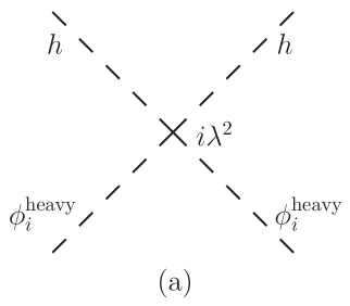
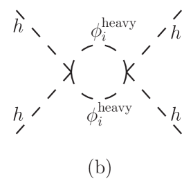
Figure 2: (a): Tree level quartic vertices involving at least two hh fields with vertex factors λ2proportional-toabsentsuperscript𝜆2\propto\lambda^{2}, in the limit tanβ1much-greater-than𝛽1\tan\beta\gg 1. In this limit, hu0h,hd0H,hs0hs0formulae-sequencesubscriptsuperscript0𝑢formulae-sequencesubscriptsuperscript0𝑑𝐻subscriptsuperscript0𝑠subscriptsuperscript0𝑠h^{0}_{u}\rightarrow h,h^{0}_{d}\rightarrow H,h^{0}_{s}\rightarrow h^{0}_{s}. No h4superscript4h^{4} quartic terms at formed at tree level. ϕisubscriptitalic-ϕ𝑖\phi_{i} correspond to the heavy fields H,hs0,AD0,AS0𝐻subscriptsuperscript0𝑠subscriptsuperscript𝐴0𝐷subscriptsuperscript𝐴0𝑆H,h^{0}_{s},A^{0}_{D},A^{0}_{S}. (b): One-loop quartic vertices with four hh legs, formed from the tree level vertices in (a). These are λ4proportional-toabsentsuperscript𝜆4\propto\lambda^{4} and account for most of the radiative corrections to the Higgs mass in our model.

We could gain an intuitive understanding of our results by qualitatively estimating the size of the one-loop radiative corrections without recourse to the effective potential. Such an estimate would serve as a useful cross-check of the results obtained from ΔVΔ𝑉\Delta V. We do this by the following argument in our limit of interest, tanβ1much-greater-than𝛽1\tan\beta\gg 1 and λgmuch-greater-than𝜆𝑔\lambda\gg g. In this limit, we identify the real scalars hu0h,hd0H,hs0hs0formulae-sequencesubscriptsuperscript0𝑢formulae-sequencesubscriptsuperscript0𝑑𝐻subscriptsuperscript0𝑠subscriptsuperscript0𝑠h^{0}_{u}\rightarrow h,~{}h^{0}_{d}\rightarrow H,~{}h^{0}_{s}\rightarrow h^{0}_{s}, where hh is the SM Higgs boson, and H𝐻H and hs0subscriptsuperscript0𝑠h^{0}_{s} are non-standard Higgses. The Standard Model Higgs and the Goldstone bosons reside mostly in Husubscript𝐻𝑢H_{u} and the non-standard CP-even and CP-odd Higgses in Hdsubscript𝐻𝑑H_{d} and S𝑆S.

For λgmuch-greater-than𝜆𝑔\lambda\gg g, the most important quartic terms at tree-level are those proportional to λ2superscript𝜆2\lambda^{2}. Before EWSB, we can read them off from Eq. (18) as the terms |Hu0|2|Hd0|2superscriptsuperscriptsubscript𝐻𝑢02superscriptsuperscriptsubscript𝐻𝑑02|H_{u}^{0}|^{2}|H_{d}^{0}|^{2}, Hu0Hd0Hu+Hdsuperscriptsubscript𝐻𝑢0superscriptsubscript𝐻𝑑0subscriptsuperscript𝐻𝑢subscriptsuperscript𝐻𝑑H_{u}^{0}H_{d}^{0}H^{+}_{u}H^{-}_{d}, |Hu0|2|S|2superscriptsuperscriptsubscript𝐻𝑢02superscript𝑆2|H_{u}^{0}|^{2}|S|^{2} and |Hd0|2|S|2superscriptsuperscriptsubscript𝐻𝑑02superscript𝑆2|H_{d}^{0}|^{2}|S|^{2}. After EWSB, we can expand Hu,Hd,Ssubscript𝐻𝑢subscript𝐻𝑑𝑆H_{u},H_{d},S using Eq. (25) to obtain various quartic vertices in terms of the real and charged scalars.

Fig. 2(a) shows all the tree-level quartic vertices that involve at least two hh fields. Recall that the SM Higgs mass is set by the coupling strength of the quartic term h4superscript4h^{4} in the scalar potential. The tree-level λ𝜆\lambda-dependent quartic h4superscript4h^{4} terms are suppressed at large tanβ𝛽\tan\beta. However, using the vertices in Fig. 2(a), we can construct four one-loop level quartic vertices proportional to h4superscript4h^{4}, as shown in Fig. 2(b). Each of these diagrams is proportional to λ4log(MAi2/MZ2)superscript𝜆4subscriptsuperscript𝑀2subscript𝐴𝑖subscriptsuperscript𝑀2𝑍\lambda^{4}\log(M^{2}_{A_{i}}/M^{2}_{Z}), where MAi2subscriptsuperscript𝑀2subscript𝐴𝑖M^{2}_{A_{i}} is the mass scale of the heavy field running in the loop. Two diagrams each correspond to MAD2subscriptsuperscript𝑀2subscript𝐴𝐷M^{2}_{A_{D}} and MAS2subscriptsuperscript𝑀2subscript𝐴𝑆M^{2}_{A_{S}} respectively. Since the internal propagators are identical, each diagram comes with a factor of 2. Canonical normalization of the mass term of a real scalar implies an additional factor of 1/2121/2. Finally, including the loop factor 1/16π2116superscript𝜋21/16\pi^{2}, we find the approximate correction to the lightest CP-even eigenstate to be

Πhh1222λ416π2[log(MAD2MZ2)+log(MAS2MZ2)],subscriptΠ1222superscript𝜆416superscript𝜋2delimited-[]subscriptsuperscript𝑀2subscript𝐴𝐷subscriptsuperscript𝑀2𝑍subscriptsuperscript𝑀2subscript𝐴𝑆subscriptsuperscript𝑀2𝑍\displaystyle\Pi_{hh}\approx\frac{1}{2}\cdot\frac{2\cdot 2\cdot\lambda^{4}}{16\pi^{2}}\left[\log\left(\frac{M^{2}_{A_{D}}}{M^{2}_{Z}}\right)+\log\left(\frac{M^{2}_{A_{S}}}{M^{2}_{Z}}\right)\right], (38)

which agrees with Eq. (37).

It would be interesting to compare the Higgs mass corrections obtained from the heavy Higgs fields and those obtained from top squarks. For simplicity, let us set the pseudoscalar masses equal, MA=MAD=MASsubscript𝑀𝐴subscript𝑀subscript𝐴𝐷subscript𝑀subscript𝐴𝑆M_{A}=M_{A_{D}}=M_{A_{S}}, and obtain

Πhhhiggs=λ44π2v2log(MA2MZ2).subscriptsuperscriptΠhiggssuperscript𝜆44superscript𝜋2superscript𝑣2subscriptsuperscript𝑀2𝐴subscriptsuperscript𝑀2𝑍\displaystyle\Pi^{\rm higgs}_{hh}=\frac{\lambda^{4}}{4\pi^{2}}v^{2}\log\left(\frac{M^{2}_{A}}{M^{2}_{Z}}\right). (39)

Again for simplicity, we can assume the top squarks are degenerate (mt~=mt1~=mt2~subscript𝑚~𝑡subscript𝑚~subscript𝑡1subscript𝑚~subscript𝑡2m_{\tilde{t}}=m_{\tilde{t_{1}}}=m_{\tilde{t_{2}}}). Then we obtain [43]

Πhhstops=3yt44π2v2log(mt~2MZ2).subscriptsuperscriptΠstops3subscriptsuperscript𝑦4𝑡4superscript𝜋2superscript𝑣2subscriptsuperscript𝑚2~𝑡subscriptsuperscript𝑀2𝑍\displaystyle\Pi^{\rm stops}_{hh}=\frac{3y^{4}_{t}}{4\pi^{2}}v^{2}\log\left(\frac{m^{2}_{\tilde{t}}}{M^{2}_{Z}}\right). (40)

The factor of 3 arises from the three QCD colors. If the pseudoscalars and the top squark are degenerate (MA=mt~subscript𝑀𝐴subscript𝑚~𝑡M_{A}=m_{\tilde{t}}), we find from Eqs. (39) and (40) that Πhhhiggs>ΠhhstopssubscriptsuperscriptΠhiggssimilar-tosubscriptsuperscriptΠstops\Pi^{\rm higgs}_{hh}\begin{array}[]{c}\sim\vspace{-21pt}\\ >\end{array}\Pi^{\rm stops}_{hh} for λ>31/4yt𝜆similar-tosuperscript314subscript𝑦𝑡\lambda\begin{array}[]{c}\sim\vspace{-21pt}\\ >\end{array}3^{1/4}y_{t}. Since yt=mt/v1subscript𝑦𝑡subscript𝑚𝑡𝑣similar-to-or-equals1y_{t}=m_{t}/v\simeq 1, we have Πhhhiggs>ΠhhstopssubscriptsuperscriptΠhiggssimilar-tosubscriptsuperscriptΠstops\Pi^{\rm higgs}_{hh}\begin{array}[]{c}\sim\vspace{-21pt}\\ >\end{array}\Pi^{\rm stops}_{hh} for λ>1.3𝜆similar-to1.3\lambda\begin{array}[]{c}\sim\vspace{-21pt}\\ >\end{array}1.3.

In the discussion of our model’s phenomenology, we set mt~=800GeVsubscript𝑚~𝑡800GeVm_{\tilde{t}}=800~{}\text{GeV} while MAsubscript𝑀𝐴M_{A} ranges between 4 TeV and 8 TeV; therefore, the one-loop corrections from the Higgs sector dominate those from the stops. Hence, throughout our analysis, the effect of the top squark correction to the SM Higgs mass is neglected.
Refer to caption
Refer to caption
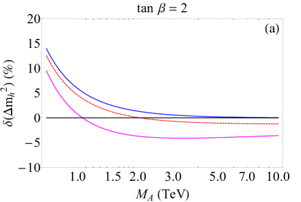
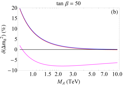
Figure 3: Discrepancies between the Higss mass radiative corrections obtained from our one-loop effective potential in Eq. (2.2.2) and those obtained by other means, as a function of the mass MAsubscript𝑀𝐴M_{A} of degenerate pseudoscalars. The blue, dashed red and magenta curves represent corrections obtained from Eq. (36), Eq. (38) and Ref. [35] respectively. (a) corresponds to tanβ=2𝛽2\tan\beta=2, (b) corresponds to tanβ=50𝛽50\tan\beta=50. See text for details of the behavior of the curves.

We can now quantify the discrepancies between the results obtained by a full one-loop effective potential calculation and those obtained by other means. To do so, first we compute the correction to the Higgs squared mass obtained from Eq. (2.2.2), and denote it by Δmh2Δsubscriptsuperscript𝑚2\Delta m^{2}_{h}. For the same set of parameters, we compute (Δmh2)isubscriptΔsubscriptsuperscript𝑚2𝑖(\Delta m^{2}_{h})_{i} for each alternative approximation labelled by i𝑖i. We then take the difference and normalize it to Δmh2Δsubscriptsuperscript𝑚2\Delta m^{2}_{h} and define the discrepancy as

δ(Δmh2)=(Δmh2)iΔmh2Δmh2,𝛿Δsubscriptsuperscript𝑚2subscriptΔsubscriptsuperscript𝑚2𝑖Δsubscriptsuperscript𝑚2Δsubscriptsuperscript𝑚2\displaystyle\delta(\Delta m^{2}_{h})={(\Delta m^{2}_{h})_{i}-\Delta m^{2}_{h}\over\Delta m^{2}_{h}}, (41)

which is then expressed as a percentage. This approach eliminates the λ𝜆\lambda-dependence of the discrepancies and allows us to focus on their behavior with respect to tanβ𝛽\tan\beta and the heavy (pseudo)scalar masses.

Assuming for simplicity that the CP-odd scalars are degenerate, we depict in Fig. 3 the discrepancies as a function of MAsubscript𝑀𝐴M_{A}. Figs. 3(a) and 3(b) correspond to tanβ=2𝛽2\tan\beta=2 and tanβ=50𝛽50\tan\beta=50 respectively. The blue curve denotes (Δmh2)isubscriptΔsubscriptsuperscript𝑚2𝑖(\Delta m^{2}_{h})_{i} obtained from the approximation in Eq. (36). Since this approximation neglects doublet-singlet mixing, it tends to overestimate the correction, i.e., δ(Δmh2)>0𝛿Δsubscriptsuperscript𝑚20\delta(\Delta m^{2}_{h})>0 as observed in the plot. The discrepancy is also seen to asymptote to zero at large MAsubscript𝑀𝐴M_{A}, where the CP-even singlet Higgs decouples from the SM Higgs. The dashed red curve is (Δmh2)isubscriptΔsubscriptsuperscript𝑚2𝑖(\Delta m^{2}_{h})_{i} obtained from our qualitative diagrammatic estimate (Eq. (37)). Since the estimate is designed for large tanβ𝛽\tan\beta it disagrees with the blue curve at tanβ=2𝛽2\tan\beta=2, but coincides with it very well at tanβ=50𝛽50\tan\beta=50. The magenta curve depicts (Δmh2)isubscriptΔsubscriptsuperscript𝑚2𝑖(\Delta m^{2}_{h})_{i} obtained from NMSSMTools 4.5.1 [35, 43], which also computes the one-loop radiative corrections from the effective potential, albeit under a different set of approximations. We find an interesting discrepancy here, to which we now turn.

The eigenvalues of the CP-odd mass matrix in Eq. (28) are given by

E±2=12(T±T24D),subscriptsuperscript𝐸2plus-or-minus12plus-or-minus𝑇superscript𝑇24𝐷\displaystyle E^{2}_{\pm}={1\over 2}\left(T\pm\sqrt{T^{2}-4D}\right), (42)

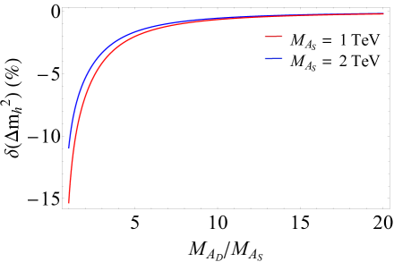
where T=(MA2)11+(MA2)22𝑇subscriptsubscriptsuperscript𝑀2𝐴11subscriptsubscriptsuperscript𝑀2𝐴22T=\left(M^{2}_{A}\right)_{11}+\left(M^{2}_{A}\right)_{22} is the trace and D=(MA2)11(MA2)22(MA2)122𝐷subscriptsubscriptsuperscript𝑀2𝐴11subscriptsubscriptsuperscript𝑀2𝐴22subscriptsuperscriptsubscriptsuperscript𝑀2𝐴212D=\left(M^{2}_{A}\right)_{11}\left(M^{2}_{A}\right)_{22}-\left(M^{2}_{A}\right)^{2}_{12} is the determinant of the mass matrix. In Ref. [35], it is assumed that DT2much-less-than𝐷superscript𝑇2D\ll T^{2}, so that the eigenmasses are obtained as E+2T,E2D/Tformulae-sequencesimilar-to-or-equalssubscriptsuperscript𝐸2𝑇similar-to-or-equalssubscriptsuperscript𝐸2𝐷𝑇E^{2}_{+}\simeq T,~{}E^{2}_{-}\simeq D/T. This always leads to a hierarchy between the pseudoscalar masses. In contrast, our approach sets the off-diagonal element (MA2)12subscriptsubscriptsuperscript𝑀2𝐴12\left(M^{2}_{A}\right)_{12} to zero so that the eigenmasses are E+2=MAD2=(MA2)11,E2=MAS2=(MA2)22formulae-sequencesubscriptsuperscript𝐸2subscriptsuperscript𝑀2subscript𝐴𝐷subscriptsubscriptsuperscript𝑀2𝐴11subscriptsuperscript𝐸2subscriptsuperscript𝑀2subscript𝐴𝑆subscriptsubscriptsuperscript𝑀2𝐴22E^{2}_{+}=M^{2}_{A_{D}}=\left(M^{2}_{A}\right)_{11},~{}E^{2}_{-}=M^{2}_{A_{S}}=\left(M^{2}_{A}\right)_{22}. Therefore, our approach allows for a variety of mass splittings. Hence the discrepancy between us and Ref. [35] is expected to be maximum when the CP-odd Higgses are degenerate, and minimum when these masses are well split. We illustrate this effect in Fig. 4. Since (MA2)12=0subscriptsubscriptsuperscript𝑀2𝐴120\left(M^{2}_{A}\right)_{12}=0 in our approach, we set (MA2)12subscriptsubscriptsuperscript𝑀2𝐴12\left(M^{2}_{A}\right)_{12} to zero in the expression of Ref. [35] as well, in order to make an “apples-to-apples” comparison. We then plot δ(Δmh2)𝛿Δsubscriptsuperscript𝑚2\delta(\Delta m^{2}_{h}) as a function of MAD/MASsubscript𝑀subscript𝐴𝐷subscript𝑀subscript𝐴𝑆M_{A_{D}}/M_{A_{S}}, where we have taken λ=1.25𝜆1.25\lambda=1.25, tanβ=50𝛽50\tan\beta=50 and μeff=110GeVsubscript𝜇eff110GeV\mu_{\text{eff}}=110~{}\text{GeV}. The red and blue curves depict MAS=1TeVsubscript𝑀subscript𝐴𝑆1TeVM_{A_{S}}=1~{}\text{TeV} and MAS=2TeVsubscript𝑀subscript𝐴𝑆2TeVM_{A_{S}}=2~{}\text{TeV} respectively. As expected, we find the discrepancy at its greatest at MAD/MAS=1subscript𝑀subscript𝐴𝐷subscript𝑀subscript𝐴𝑆1M_{A_{D}}/M_{A_{S}}=1, which can reach upto 15%similar-toabsentpercent15\sim 15\%. Observe also that δ(Δmh2)<0𝛿Δsubscriptsuperscript𝑚20\delta(\Delta m^{2}_{h})<0, implying that Ref. [35] underestimates the one-loop contribution to the Higgs mass in the region around MAD/MAS=1subscript𝑀subscript𝐴𝐷subscript𝑀subscript𝐴𝑆1M_{A_{D}}/M_{A_{S}}=1. As we raise MAD/MASsubscript𝑀subscript𝐴𝐷subscript𝑀subscript𝐴𝑆M_{A_{D}}/M_{A_{S}}, the discrepancy drops quickly and our results concur.

The results of Ref. [35] were originally used in the code of NMSSMTools 4.5.1 [43]. Since our phenomenology in Section 3 assumes MAD=MASsubscript𝑀subscript𝐴𝐷subscript𝑀subscript𝐴𝑆M_{A_{D}}=M_{A_{S}}, we replaced the code in NMSSMTools 4.5.1 with the expressions that we derived in Appendix B.
Refer to caption
Figure 4: The discrepancy between Higgs mass corrections obtained by Ref. [35] (which were used in the original code of NMSSMTools 4.5.1) and by us, as a function of the ratio of the heavy CP-odd Higgs masses. The red (blue) curve corresponds to MAS=1(2)TeVsubscript𝑀subscript𝐴𝑆12TeVM_{A_{S}}=1(2)~{}\text{TeV}. The discrepancy arises due to an approximation assumed by Ref. [35], namely, that a hierarchy exists in the pseudoscalar spectrum. It is seen that our results agree when there is indeed a hierarchy. See text for more details.

2.2.3 Stability of the electroweak scale

The minimization conditions of the tree level Higgs potential in Eq. (17) lead to the same relation between the electroweak scale and the SUSY parameters seen in the MSSM. In particular, the EWSB condition is [44]

MZ2=tβ2+1tβ21(mHd2mHu2)(mHu2+mHd2)2|μeff|2,superscriptsubscript𝑀𝑍2superscriptsubscript𝑡𝛽21superscriptsubscript𝑡𝛽21superscriptsubscript𝑚subscript𝐻𝑑2superscriptsubscript𝑚subscript𝐻𝑢2superscriptsubscript𝑚subscript𝐻𝑢2superscriptsubscript𝑚subscript𝐻𝑑22superscriptsubscript𝜇eff2\displaystyle M_{Z}^{2}=\frac{t_{\beta}^{2}+1}{t_{\beta}^{2}-1}\left(m_{H_{d}}^{2}-m_{H_{u}}^{2}\right)-\left(m_{H_{u}}^{2}+m_{H_{d}}^{2}\right)-2\left|\mu_{\text{eff}}\right|^{2}, (43)

which at large tanβ𝛽\tan\beta reduces to

12MZ2mHu2|μeff|2,12superscriptsubscript𝑀𝑍2superscriptsubscript𝑚subscript𝐻𝑢2superscriptsubscript𝜇eff2\displaystyle\frac{1}{2}M_{Z}^{2}\approx-m_{H_{u}}^{2}-\left|\mu_{\text{eff}}\right|^{2}, (44)

where the mHd2superscriptsubscript𝑚subscript𝐻𝑑2m_{H_{d}}^{2} terms are suppressed by tβ1superscriptsubscript𝑡𝛽1t_{\beta}^{-1}. With this result we can now quantify the relative importance of different contributions (denoted by a𝑎a) to the EWSB scale (MZ2/2superscriptsubscript𝑀𝑍22M_{Z}^{2}/2) as

Δ(a2)=|a2MZ2/2|.Δsuperscript𝑎2superscript𝑎2superscriptsubscript𝑀𝑍22\displaystyle\Delta(a^{2})=\left|\frac{a^{2}}{M_{Z}^{2}/2}\right|. (45)

The tree-level and one-loop corrections are the same as in the MSSM and are well-known [45]. For instance, the tree-level contribution due to μeff< 350superscriptsimilar-tosubscript𝜇eff350\mu_{\text{eff}}\>\raisebox{-2.15277pt}{$\stackrel{{\scriptstyle\textstyle<}}{{\sim}}$}\>350 GeV is equivalent to the one-loop contribution of stops at mt~< 800superscriptsimilar-tosubscript𝑚~𝑡800m_{\tilde{t}}\>\raisebox{-2.15277pt}{$\stackrel{{\scriptstyle\textstyle<}}{{\sim}}$}\>800 GeV [46]. Hence the regions we are considering in this article are typically as tuned as regions of the MSSM with a light stop.

2.2.4 Higgs couplings to SM particles

LHC measurements of signal strengths (production rate ×\times branching ratio) can potentially constrain the properties of the Higgs sector. Mixing among the Higgs fields can in principle alter the lightest Higgs boson’s SM-like behavior. We follow the analysis of Ref. [30] to apply the relevant limits.

After including the one-loop self-energy corrections, we rotate the Higgs fields (hu0,hd0,hs0)subscriptsuperscript0𝑢subscriptsuperscript0𝑑subscriptsuperscript0𝑠(h^{0}_{u},h^{0}_{d},h^{0}_{s}) into the mass eigenbasis (h1,h2,h3)subscript1subscript2subscript3(h_{1},h_{2},h_{3}) and identify the lightest scalar as

h1=(hu0sinα+hd0cosα)cosγ+hs0sinγ,subscript1subscriptsuperscript0𝑢𝛼subscriptsuperscript0𝑑𝛼𝛾subscriptsuperscript0𝑠𝛾\displaystyle h_{1}=(-h^{0}_{u}~{}\sin\alpha+h^{0}_{d}~{}\cos\alpha)\cos\gamma+h^{0}_{s}~{}\sin\gamma, (46)

where the angles α𝛼\alpha is the usual MSSM CP-even mixing angle that characterizes doublet-doublet mixing and γ𝛾\gamma characterizes the doublet-singlet mixing. We can then write down the reduced couplings of h1subscript1h_{1} to pairs of fermions and vector bosons as

gtth1gtthSMsubscript𝑔𝑡𝑡subscript1subscript𝑔𝑡𝑡subscriptSM\displaystyle{g_{tth_{1}}\over g_{tth_{\rm SM}}} =\displaystyle= cosγ(cosδ+sinδtanβ),𝛾𝛿𝛿𝛽\displaystyle\cos\gamma\left(\cos\delta+{\sin\delta\over\tan\beta}\right),
gbbh1gbbhSMsubscript𝑔𝑏𝑏subscript1subscript𝑔𝑏𝑏subscriptSM\displaystyle{g_{bbh_{1}}\over g_{bbh_{\rm SM}}} =\displaystyle= cosγ(cosδsinδtanβ),𝛾𝛿𝛿𝛽\displaystyle\cos\gamma(\cos\delta-\sin\delta\tan\beta),
gVVh1gVVhSMsubscript𝑔𝑉𝑉subscript1subscript𝑔𝑉𝑉subscriptSM\displaystyle{g_{VVh_{1}}\over g_{VVh_{\rm SM}}} =\displaystyle= cosγcosδ,𝛾𝛿\displaystyle\cos\gamma\cos\delta, (47)

where δ=αβ+π/2𝛿𝛼𝛽𝜋2\delta=\alpha-\beta+\pi/2.

If we inspect the off-diagonal entries of Eq. (31), we see that for AλMAmuch-less-thansubscript𝐴𝜆subscript𝑀𝐴A_{\lambda}\ll M_{A} and large tanβ𝛽\tan\beta, (MH2)hH<(MH2)hSsubscriptsubscriptsuperscript𝑀2𝐻𝐻subscriptsubscriptsuperscript𝑀2𝐻𝑆\left(M^{2}_{H}\right)_{hH}<\left(M^{2}_{H}\right)_{hS}. Thus as we raise MAsubscript𝑀𝐴M_{A}, the heavy doublet Higgs (identified as h3subscript3h_{3}) generally decouples faster than the heavy singlet (identified as h2subscript2h_{2}), as noted by Refs. [25, 31] In dealing with the phenomenological consequences of our model, we focus exactly on the region of AλMAmuch-less-thansubscript𝐴𝜆subscript𝑀𝐴A_{\lambda}\ll M_{A} and large tanβ𝛽\tan\beta. Therefore for the rest of this analysis we assume h3subscript3h_{3} is decoupled from the spectrum and h2subscript2h_{2} is not. In this limit, the mixing angle γ𝛾\gamma is given by

sin2γ=mhh2mh12mh22mh12,superscript2𝛾subscriptsuperscript𝑚2subscriptsuperscript𝑚2subscript1subscriptsuperscript𝑚2subscript2subscriptsuperscript𝑚2subscript1\displaystyle\sin^{2}\gamma={m^{2}_{hh}-m^{2}_{h_{1}}\over m^{2}_{h_{2}}-m^{2}_{h_{1}}}, (48)

where mhh2=λ2v2sin22β+MZ2cos22βsubscriptsuperscript𝑚2superscript𝜆2superscript𝑣2superscript22𝛽subscriptsuperscript𝑀2𝑍superscript22𝛽m^{2}_{hh}=\lambda^{2}v^{2}\sin^{2}2\beta+M^{2}_{Z}\cos^{2}2\beta, and the Higgs couplings to fermions and vector bosons become

gtth1gtthSM=gbbh1gbbhSM=gVVh1gVVhSM=cosγ.subscript𝑔𝑡𝑡subscript1subscript𝑔𝑡𝑡subscriptSMsubscript𝑔𝑏𝑏subscript1subscript𝑔𝑏𝑏subscriptSMsubscript𝑔𝑉𝑉subscript1subscript𝑔𝑉𝑉subscriptSM𝛾\displaystyle{g_{tth_{1}}\over g_{tth_{\rm SM}}}={g_{bbh_{1}}\over g_{bbh_{\rm SM}}}={g_{VVh_{1}}\over g_{VVh_{\rm SM}}}=\cos\gamma. (49)

Using these relations Ref. [30] performed a universal fit on the LHC signal strength measurements and found that sin2γ0.23superscript2𝛾0.23\sin^{2}\gamma\leq 0.23 at 95% C.L. This result was obtained using tree level relations for the reduced couplings. When we include our one-loop corrections, we find that the reduced couplings are modified by less than 1%percent11\%. Therefore, in the discussion of our model’s phenomenology in Section 3 we will simply use the results of Ref. [30] to constrain the Higgs couplings with LHC measurements.

2.3 Neutralino sector

The composition of the lightest neutralino and its couplings to the Higgs sector is central to the dark matter phenomenology of our model. The neutralino mass matrix in the basis (B~,W~,ψ~d0,ψ~u0,ψ~s0~𝐵~𝑊subscriptsuperscript~𝜓0𝑑subscriptsuperscript~𝜓0𝑢subscriptsuperscript~𝜓0𝑠\widetilde{B},\widetilde{W},\widetilde{\psi}^{0}_{d},\widetilde{\psi}^{0}_{u},\widetilde{\psi}^{0}_{s}) is given by

neut=(M10g1vcosβ/2g1vsinβ/200M2g2vcosβ/2g2vsinβ/20g1vcosβ/2g2vcosβ/20μeffλvsinβg1vsinβ/2g2vsinβ/2μeff0λvcosβ00λvsinβλvcosβμ)subscriptneutsubscript𝑀10subscript𝑔1𝑣𝛽2subscript𝑔1𝑣𝛽200subscript𝑀2subscript𝑔2𝑣𝛽2subscript𝑔2𝑣𝛽20subscript𝑔1𝑣𝛽2subscript𝑔2𝑣𝛽20subscript𝜇eff𝜆𝑣𝛽subscript𝑔1𝑣𝛽2subscript𝑔2𝑣𝛽2subscript𝜇eff0𝜆𝑣𝛽00𝜆𝑣𝛽𝜆𝑣𝛽superscript𝜇\mathcal{M_{\text{neut}}}=\left(\begin{array}[]{ccccc}M_{1}&0&-g_{1}v\cos\beta/\sqrt{2}&g_{1}v\sin\beta/\sqrt{2}&0\\ 0&M_{2}&g_{2}v\cos\beta/\sqrt{2}&-g_{2}v\sin\beta/\sqrt{2}&0\\ -g_{1}v\cos\beta/\sqrt{2}&g_{2}v\cos\beta/\sqrt{2}&0&-\mu_{\text{eff}}&-\lambda v\sin\beta\\ g_{1}v\sin\beta/\sqrt{2}&-g_{2}v\sin\beta/\sqrt{2}&-\mu_{\text{eff}}&0&-\lambda v\cos\beta\\ 0&0&-\lambda v\sin\beta&-\lambda v\cos\beta&\mu^{\prime}\\ \end{array}\right) (50)

Notice that when μM1,M2,μeffmuch-less-thansuperscript𝜇subscript𝑀1subscript𝑀2subscript𝜇eff\mu^{\prime}\ll M_{1},M_{2},\mu_{\text{eff}}, large λ𝜆\lambda couplings imply a large Higgsino component in the lightest neutralino. This feature has many unique consequences for the dark matter phenomenology discussed in Sec. 3. As we shall see, the Higgs-χ~10subscriptsuperscript~𝜒01\widetilde{\chi}^{0}_{1}-χ~10subscriptsuperscript~𝜒01\widetilde{\chi}^{0}_{1} coupling strengh plays an important role in constraining our model with dark matter experiments. This coupling, denoted hereafter by ghχχsubscript𝑔𝜒𝜒g_{h\chi\chi}, is obtained as

ghχχ=λ2(ζHuNψ~d0Nψ~s0+ζHdNψ~u0Nψ~s0+ζSNψ~u0Nψ~d0)g12NB~(ζHuNψ~d0ζHdNψ~u0),subscript𝑔𝜒𝜒𝜆2subscript𝜁subscript𝐻𝑢subscript𝑁subscriptsuperscript~𝜓0𝑑subscript𝑁subscriptsuperscript~𝜓0𝑠subscript𝜁subscript𝐻𝑑subscript𝑁subscriptsuperscript~𝜓0𝑢subscript𝑁subscriptsuperscript~𝜓0𝑠subscript𝜁𝑆subscript𝑁subscriptsuperscript~𝜓0𝑢subscript𝑁subscriptsuperscript~𝜓0𝑑subscript𝑔12subscript𝑁~𝐵subscript𝜁subscript𝐻𝑢subscript𝑁subscriptsuperscript~𝜓0𝑑subscript𝜁subscript𝐻𝑑subscript𝑁subscriptsuperscript~𝜓0𝑢\displaystyle g_{h\chi\chi}=\frac{\lambda}{\sqrt{2}}(\zeta_{H_{u}}N_{\widetilde{\psi}^{0}_{d}}N_{\widetilde{\psi}^{0}_{s}}+\zeta_{H_{d}}N_{\widetilde{\psi}^{0}_{u}}N_{\widetilde{\psi}^{0}_{s}}+\zeta_{S}N_{\widetilde{\psi}^{0}_{u}}N_{\widetilde{\psi}^{0}_{d}})-\frac{g_{1}}{2}N_{\widetilde{B}}(\zeta_{H_{u}}N_{\widetilde{\psi}^{0}_{d}}-\zeta_{H_{d}}N_{\widetilde{\psi}^{0}_{u}}),
(51)

where the Nisubscript𝑁𝑖N_{i} and ζjsubscript𝜁𝑗\zeta_{j} are the appropriate components of the lightest neutralino and the SM-like Higgs respectively. In terms of the rotation angles in Eq. (46), we can read off

ζHu=sinαcosγ,ζHd=cosαcosγ,ζS=sinγ.formulae-sequencesubscript𝜁subscript𝐻𝑢𝛼𝛾formulae-sequencesubscript𝜁subscript𝐻𝑑𝛼𝛾subscript𝜁𝑆𝛾\displaystyle\zeta_{H_{u}}=-\sin\alpha\cos\gamma,~{}~{}~{}~{}\zeta_{H_{d}}=\cos\alpha\cos\gamma,~{}~{}~{}~{}\zeta_{S}=\sin\gamma.

The dominant channel for χ~10subscriptsuperscript~𝜒01\widetilde{\chi}^{0}_{1}-nucleon scattering is through a t𝑡t-channel Higgs. Therefore, dark matter direct detection experiments, as well as limits on the invisible decay width of the Higgs, apply strong contraints on the coupling ghχχsubscript𝑔𝜒𝜒g_{h\chi\chi}. A suppressed ghχχsubscript𝑔𝜒𝜒g_{h\chi\chi} can occur in our model either when the Higgsino content is suppressed, making χ~10subscriptsuperscript~𝜒01\widetilde{\chi}^{0}_{1} mostly singlino or bino, or when there is a delicate cancellation between the various terms in Eq. 51. We illustrate this point in more detail in Sec. 3.
Refer to caption
Refer to caption
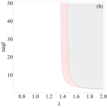
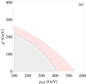
Figure 5: Limits from electroweak precision parameter T𝑇T on the neutralino sector of our model. The shaded regions are where Tχ>0.15subscript𝑇𝜒0.15T_{\chi}>0.15 and therefore excluded at 95%percent9595\% C.L. Regions shaded gray correspond to the wino decoupled from the spectrum (MW~=10TeVsubscript𝑀~𝑊10TeVM_{\tilde{W}}=10~{}\text{TeV}) and regions shaded red to MW~=200GeVsubscript𝑀~𝑊200GeVM_{\tilde{W}}=200~{}\text{GeV}. In (a), λ=1.25𝜆1.25\lambda=1.25 and tanβ=5𝛽5\tan\beta=5 and in (b), μeff=μ=300GeVsubscript𝜇effsuperscript𝜇300GeV\mu_{\text{eff}}=\mu^{\prime}=300~{}\text{GeV}. See text for details of the behavior of these curves.

2.3.1 Electroweak precision limits

Due to mixing between the Higgsinos and the singlino induced by large λ𝜆\lambda in certain regions, constraints from electroweak precision experiments can be strong in Fat Higgs/λ𝜆\lambda-SUSY models  [22, 24]. In particular, the T𝑇T parameter can get large contributions from the neutralino sector, denoted hereafter by Tχsubscript𝑇𝜒T_{\chi}. This phenomenon is understood easily in the limit where the electroweak gauginos B~~𝐵\widetilde{B} and W~~𝑊\widetilde{W} decouple from the spectrum, i.e., M1,M2subscript𝑀1subscript𝑀2M_{1},M_{2} are very large. This leaves us with three mass scales μeff,μsubscript𝜇effsuperscript𝜇\mu_{\text{eff}},\mu^{\prime} and λv𝜆𝑣\lambda v, which set the mass of the lightest neutralino, Mχ~10subscript𝑀subscriptsuperscript~𝜒01M_{\tilde{\chi}^{0}_{1}}. The lightest chargino is mostly Higgsino with a mass μeffsubscript𝜇eff\mu_{\text{eff}}. In this limit, Tχsubscript𝑇𝜒T_{\chi} is large when Mχ~1±Mχ~10subscript𝑀subscriptsuperscript~𝜒plus-or-minus1subscript𝑀subscriptsuperscript~𝜒01M_{\tilde{\chi}^{\pm}_{1}}-M_{\tilde{\chi}^{0}_{1}} is large and when there is as a significant Higgsino component in χ~10subscriptsuperscript~𝜒01\widetilde{\chi}^{0}_{1}. For simplicity, let us work in the limit where tanβ𝛽\tan\beta is large. Then the neutralino mass matrix in Eq. (50) is simply

neut(0μeffλvμeff00λv0μ).similar-tosubscriptneut0subscript𝜇eff𝜆𝑣subscript𝜇eff00𝜆𝑣0superscript𝜇\mathcal{M_{\text{neut}}}\sim\left(\begin{array}[]{ccc}0&-\mu_{\text{eff}}&-\lambda v\\ -\mu_{\text{eff}}&0&0\\ -\lambda v&0&\mu^{\prime}\\ \end{array}\right). (52)

Tχsubscript𝑇𝜒T_{\chi} is suppressed either when μμeffλvsimilar-tosuperscript𝜇subscript𝜇effsimilar-to𝜆𝑣\mu^{\prime}\sim\mu_{\text{eff}}\sim\lambda v, where Mχ~1±Mχ~10subscript𝑀subscriptsuperscript~𝜒plus-or-minus1subscript𝑀subscriptsuperscript~𝜒01M_{\tilde{\chi}^{\pm}_{1}}-M_{\tilde{\chi}^{0}_{1}} is small, or when μeffμλvmuch-greater-thansubscript𝜇effsuperscript𝜇similar-to𝜆𝑣\mu_{\text{eff}}\gg\mu^{\prime}\sim\lambda v, where the Higgsino component in χ~10subscriptsuperscript~𝜒01\widetilde{\chi}^{0}_{1} is suppressed. For μμeffλvmuch-less-thansuperscript𝜇subscript𝜇effsimilar-to𝜆𝑣\mu^{\prime}\ll\mu_{\text{eff}}\sim\lambda v, where both Mχ~1±Mχ~10subscript𝑀subscriptsuperscript~𝜒plus-or-minus1subscript𝑀subscriptsuperscript~𝜒01M_{\tilde{\chi}^{\pm}_{1}}-M_{\tilde{\chi}^{0}_{1}} and the Higgsino component in χ~10subscriptsuperscript~𝜒01\widetilde{\chi}^{0}_{1} are large, constraints from Tχsubscript𝑇𝜒T_{\chi} can be strong.

Lowering the mass of the wino triplet M2subscript𝑀2M_{2} to μeffλvsimilar-toabsentsubscript𝜇effsimilar-to𝜆𝑣\sim\mu_{\text{eff}}\sim\lambda v can have a significant impact on Tχsubscript𝑇𝜒T_{\chi}. This is because the wino would mix with the light neutralinos and charginos. Lowering the bino mass M1subscript𝑀1M_{1}, on the other hand, gives only a negligible contribution to Tχsubscript𝑇𝜒T_{\chi}. This is because the bino mixing with the rest of the neutralinos is only proportional to g1subscript𝑔1g_{1}.333 It must be remembered that relative minus signs between μeff,μsubscript𝜇effsuperscript𝜇\mu_{\text{eff}},\mu^{\prime} and MW~subscript𝑀~𝑊M_{\tilde{W}} would introduce quantitative changes in the picture owing to new phases in the neutralino mixing angles. We will not include these relative signs in our discussion.

In Fig. 5 we present the T𝑇T-parameter contributions from the charginos and neutralinos, which were computed using the general expressions provided in Ref. [50]. In Fig. 5(a), we take λ=1.25𝜆1.25\lambda=1.25 and tanβ=5𝛽5\tan\beta=5 and show our results in the μeffμsubscript𝜇effsuperscript𝜇\mu_{\text{eff}}-\mu^{\prime} plane. The shaded regions denote where Tχsubscript𝑇𝜒T_{\chi} is not within the 95% C.L range [.01,0.15].010.15[-.01,0.15] set by the Particle Data Group [51]. The gray region corresponds to large gaugino masses (M1,M2)=(10 TeV,10 TeV)subscript𝑀1subscript𝑀210 TeV10 TeV(M_{1},M_{2})=(10\mbox{ TeV},10\mbox{ TeV}) while the red region corresponds to a light wino with (M1,M2)=(10 TeV,0.2 TeV)subscript𝑀1subscript𝑀210 TeV0.2 TeV(M_{1},M_{2})=(10\mbox{ TeV},0.2\mbox{ TeV}). As discussed above, lowering the wino mass can lead to a larger Tχsubscript𝑇𝜒T_{\chi}. For small μsuperscript𝜇\mu^{\prime}, Tχsubscript𝑇𝜒T_{\chi} decreases as μeffsubscript𝜇eff\mu_{\text{eff}} increases due to a reduction in the Higgsino component of the lightest neutralino. Similarly, raising μsuperscript𝜇\mu^{\prime} has the effect of reducing the splittings between the neutralinos and charginos which also leads to a smaller Tχsubscript𝑇𝜒T_{\chi}.

The effects of varying λ𝜆\lambda and tanβ𝛽\tan\beta on Tχsubscript𝑇𝜒T_{\chi} are presented in Fig. 5(b). Here we fix μeff=μ=300subscript𝜇effsuperscript𝜇300\mu_{\text{eff}}=\mu^{\prime}=300 GeV. The colored regions have the same definition as those in Fig. 5(a). Since the elements of neutsubscriptneut\mathcal{M_{\text{neut}}} quickly asymptote to fixed values as a function of tanβ𝛽\tan\beta, it can be seen that Tχsubscript𝑇𝜒T_{\chi} is insensitive to large tanβ𝛽\tan\beta. This insensitivity to large tanβ𝛽\tan\beta is clear in the relation derived in Ref. [22]

Tχ(tβ21tβ2+1)2F(μeff,μ,λ),subscript𝑇𝜒superscriptsuperscriptsubscript𝑡𝛽21superscriptsubscript𝑡𝛽212𝐹subscript𝜇effsuperscript𝜇𝜆\displaystyle T_{\chi}\approx\left(\frac{t_{\beta}^{2}-1}{t_{\beta}^{2}+1}\right)^{2}F(\mu_{\rm eff},\mu^{\prime},\lambda), (53)

where F(μeff,μ,λ)𝐹subscript𝜇effsuperscript𝜇𝜆F(\mu_{\rm eff},\mu^{\prime},\lambda) is some function of these variables. This relation also shows that Tχsubscript𝑇𝜒T_{\chi} is suppressed as tβsubscript𝑡𝛽t_{\beta} approaches 1, thereby allowing for larger values of λ𝜆\lambda. As stated before, lowering M2subscript𝑀2M_{2} typically increases the neutralino and chargino contributions to the T𝑇T-parameter. However, it is important to emphasize that increasing either μeffsubscript𝜇eff\mu_{\text{eff}} or μsuperscript𝜇\mu^{\prime} can significantly lower the electroweak precision constraints even for large tanβ𝛽\tan\beta. A large μeffsubscript𝜇eff\mu_{\text{eff}} comes at the cost of a slight increase in electroweak fine-tuning, but can greatly weaken T𝑇T-parameter constraints.

Finally, we make two remarks. First, the S𝑆S-parameter was not discussed here. This is because the contributions of our model to S𝑆S are very small in our regions of interest and hence the constraints are much weaker than those on the T𝑇T-parameter. Second, the T𝑇T-parameter receives a stop-sbottom contribution, as discussed in Ref. [22]. In the limit of zero left-right mixing, this is given by

Tstsb0.05(500GeVmt~L)2subscript𝑇stsb0.05superscript500GeVsubscript𝑚subscript~𝑡𝐿2\displaystyle T_{\rm st-sb}\approx 0.05\left({500~{}\text{GeV}\over m_{\tilde{t}_{L}}}\right)^{2} (54)

In our phenomenological discussions, we will choose mt~L=800GeVsubscript𝑚subscript~𝑡𝐿800GeVm_{\tilde{t}_{L}}=800~{}\text{GeV} to suppress this contribution.

3 Phenomenology

In this section we study the phenomenological constraints on the large tanβ𝛽\tan\beta regions of the Fat Higgs/λ𝜆\lambda-SUSY models. In addition to the constraints arising from Higgs corrections discussed in the previous section, we also include limits from dark matter experiments, most importantly those set by the LUX experiment [52]. In particular, the mass and couplings of the lightest neutralino χ~10subscriptsuperscript~𝜒01\widetilde{\chi}^{0}_{1} can put strong constraints on our parameter space.

In order find phenomenologically viable regions, we modified NMSSMTools 4.5.1 [43] to include the Higgs mass corrections we computed in Sec. 2.2.2. We then made the following simplifying assumptions:

  • In the Higgs sector, we take the pseudoscalars to be degenerate, with MAD=MAS=MAsubscript𝑀subscript𝐴𝐷subscript𝑀subscript𝐴𝑆subscript𝑀𝐴M_{A_{D}}=M_{A_{S}}=M_{A}. Furthermore we assume that mS=m3=0subscriptsuperscript𝑚𝑆subscript𝑚30m^{\prime}_{S}=m_{3}=0, so that the heavy CP-even Higgs bosons are also (nearly) degenerate. The condition that the CP-odd masses are degenerate requires that (MA2)12=0subscriptsubscriptsuperscript𝑀2𝐴120\left(M^{2}_{A}\right)_{12}=0 in Eq. 28, which implies Aλ=μsubscript𝐴𝜆superscript𝜇A_{\lambda}=\mu^{\prime}. Therefore, both μsuperscript𝜇\mu^{\prime} and μeffsubscript𝜇eff\mu_{\text{eff}} control the amount of doublet-singlet mixing in Eq. (27). The only independent parameters in the Higgs sector are then: λ,μeff,μ,tanβ𝜆subscript𝜇effsuperscript𝜇𝛽\lambda,\mu_{\text{eff}},\mu^{\prime},\tan\beta and MAsubscript𝑀𝐴M_{A}.

  • In order to be safe from electroweak precision bounds, we decouple the winos at M2=10subscript𝑀210M_{2}=10 TeV, leading to an effective theory for the neutralino system with five free parameters : M1subscript𝑀1M_{1}, μeffsubscript𝜇eff\mu_{\text{eff}}, μsuperscript𝜇\mu^{\prime}, λ𝜆\lambda and tanβ𝛽\tan\beta.

  • We require μeff>104subscript𝜇eff104\mu_{\text{eff}}>104 GeV to evade the LEP II bound on charged Higgsinos [54].

  • The sleptons and the first two generations of squarks are decoupled from the low energy phenomenology and their masses set at 5 TeV, unless stated otherwise. The top squark parameters are set at mQ~3=mU~3=800subscript𝑚subscript~𝑄3subscript𝑚subscript~𝑈3800m_{\tilde{Q}_{3}}=m_{\tilde{U}_{3}}=800 GeV and At=0subscript𝐴𝑡0A_{t}=0, thereby making the stop contributions to the Higgs mass and the electroweak symmetry breaking condition in Eq. (44) small. This choice of stop masses also avoids constraints from collider searches [47, 48, 49] and, as mentioned in Sec. 2.3.1, from electroweak precision tests.

  • We choose to require the conventional upper limit tanβ60𝛽60\tan\beta\leq 60, so that yb1subscript𝑦𝑏1y_{b}\leq 1 at the weak scale. Larger values of ybsubscript𝑦𝑏y_{b} may be allowed as long they do not develop a Landau pole at a scale below that of λ𝜆\lambda.

  • We assume that the relic density of dark matter is the value determined by Planck [53]. Hence, in scenarios where Ωχh2<0.12subscriptΩ𝜒superscript20.12\Omega_{\chi}h^{2}<0.12, we assume some nonthermal mechanism for generating the observed relic abundance.

These assumptions reduce the number of independent SUSY parameters to

λ,tanβ,MA,μeff,μ,M1.𝜆𝛽subscript𝑀𝐴subscript𝜇effsuperscript𝜇subscript𝑀1\displaystyle\lambda,~{}\tan\beta,~{}M_{A},~{}\mu_{\text{eff}},~{}\mu^{\prime},~{}M_{1}~{}.

As discussed in Sec. 2.3.1, precision electroweak constraints are weak either when μsuperscript𝜇\mu^{\prime} or μeffsubscript𝜇eff\mu_{\rm eff} are large for any tanβ𝛽\tan\beta, or when μλvμeffmuch-less-thansuperscript𝜇𝜆𝑣similar-tosubscript𝜇eff\mu^{\prime}\ll\lambda v\sim\mu_{\text{eff}} at low tanβ𝛽\tan\beta. In these regions, ghχχsubscript𝑔𝜒𝜒g_{h\chi\chi} (as defined in Eq. 51) can also be found to satisfy dark matter direct detection and relic density constraints. In particular we find the following viable parametric regions.

3.1 Singlino DM: Large tanβ𝛽\tan\beta and μ<λvμeffM1superscript𝜇𝜆𝑣similar-tosubscript𝜇effmuch-less-thansubscript𝑀1\mu^{\prime}<\lambda v\sim\mu_{\text{eff}}\ll M_{1}

Large λ𝜆\lambda and large tanβ𝛽\tan\beta are a new region of parameter space that have not been emphasized in the literature before. We showed in Sec. 2.2 that this region can be compatible with the mass of the SM Higgs boson because one-loop radiative corrections to the Higgs mass are insensitive to tanβ𝛽\tan\beta at large values, and are set solely by λ𝜆\lambda and MAsubscript𝑀𝐴M_{A}. We also showed that precision electroweak constraints can be weak in this region. We now show that this region is also compatible with constraints from dark matter.

As mentioned in Sec. 2.3, it can be seen from Eq. (51) that ghχχsubscript𝑔𝜒𝜒g_{h\chi\chi} is suppressed when χ~10subscriptsuperscript~𝜒01\widetilde{\chi}^{0}_{1} is mostly singlino such that Nψ~s021similar-to-or-equalssubscriptsuperscript𝑁2subscriptsuperscript~𝜓0𝑠1N^{2}_{\widetilde{\psi}^{0}_{s}}\simeq 1. This requirement is possible when μsuperscript𝜇\mu^{\prime} is relatively small compared to the other mass scales in the neutralino mass matrix. The annihilation of χ~10subscriptsuperscript~𝜒01\widetilde{\chi}^{0}_{1} into SM fields in the early universe is generally inefficient, due to both the Z𝑍Z- and hh-mediated channels being suppressed by the small Higgsino component of χ~10subscriptsuperscript~𝜒01\widetilde{\chi}^{0}_{1}. Therefore, for the cosmological relic abundance to be below the observed value Ωχh20.12similar-to-or-equalssubscriptΩ𝜒superscript20.12\Omega_{\chi}h^{2}\simeq 0.12, we consider the mechanism of resonant annihilation and co-annihilation [59].

3.1.1 Resonant annihilation

If Mχ~10subscript𝑀subscriptsuperscript~𝜒01M_{\tilde{\chi}^{0}_{1}} happens to be close to mh/2subscript𝑚2m_{h}/2, it can undergo resonant annihilation through an s𝑠s-channel Higgs. Therefore, we set μ=62.5superscript𝜇62.5\mu^{\prime}=62.5 GeV in this scenario. We also set μeff=800subscript𝜇eff800\mu_{\text{eff}}=800 GeV, M1=1subscript𝑀11M_{1}=1 TeV, tanβ=50𝛽50\tan\beta=50 and MA=4subscript𝑀𝐴4M_{A}=4 TeV. The orange curves in Fig. 6(a) depict contours of the LSP-nucleon scattering rates, σSIsubscript𝜎SI\sigma_{\text{SI}} (in units of σ0=1045cm2subscript𝜎0superscript1045superscriptcm2\sigma_{0}=10^{-45}~{}\text{cm}^{2}), on the μeffλsubscript𝜇eff𝜆\mu_{\text{eff}}-\lambda plane. The red shaded regions are excluded by LUX at 90% C.L., and the green band corresponds to 120GeVmh130GeV120GeVsubscript𝑚130GeV120~{}\text{GeV}\leq m_{h}\leq 130~{}\text{GeV}. Contours of Tχsubscript𝑇𝜒T_{\chi} are denoted by dashed curves.

In Fig. 6(a), the dark matter-nucleon scattering rates are smaller for larger μeffsubscript𝜇eff\mu_{\text{eff}} because the Higgsino fraction in χ~10subscriptsuperscript~𝜒01\widetilde{\chi}^{0}_{1} decreases. Tχsubscript𝑇𝜒T_{\chi} is observed to rise with increasing λ𝜆\lambda due to an increase in the Higgsino fraction of χ~10subscriptsuperscript~𝜒01\widetilde{\chi}^{0}_{1}. The region around mh125similar-tosubscript𝑚125m_{h}\sim 125 GeV corresponds to Tχ0.05similar-tosubscript𝑇𝜒0.05T_{\chi}\sim 0.05, which is safe from electroweak precision constraints. This regions is also safe from invisible Higgs decay bounds since the process hχ~10χ~10subscriptsuperscript~𝜒01subscriptsuperscript~𝜒01h\rightarrow\widetilde{\chi}^{0}_{1}\widetilde{\chi}^{0}_{1} is phase space suppressed.

Refer to caption
Refer to caption
Refer to caption
Refer to caption
Figure 6: Large tanβ𝛽\tan\beta parametric scenarios for Fat Higgs/λ𝜆\lambda SUSY models. (a) Singlino resonant annihilation (μ=62.5superscript𝜇62.5\mu^{\prime}=62.5 GeV, M1=1subscript𝑀11M_{1}=1 TeV): orange curves correspond to σSIsubscript𝜎SI\sigma_{\rm SI} in units of σ0=1045cm2subscript𝜎0superscript1045superscriptcm2\sigma_{0}=10^{-45}~{}\text{cm}^{2}. The red shaded region is excluded by LUX at 90% C.L. and the green shaded region corresponds to 120GeV<mh<130GeV120GeVsubscript𝑚130GeV120~{}\text{GeV}<m_{h}<130~{}\text{GeV}. The dashed lines are contours of Tχsubscript𝑇𝜒T_{\chi}. (b) Singlino co-annihilation: orange curves and red region the same as (a). The green and gray shaded regions correspond to 120GeV<mh<130GeV120GeVsubscript𝑚130GeV120~{}\text{GeV}<m_{h}<130~{}\text{GeV} for λ=1.1𝜆1.1\lambda=1.1 and λ=1.25𝜆1.25\lambda=1.25 respectively. (c) Bino resonant annihilation (μ=1superscript𝜇1\mu^{\prime}=1 TeV, M1=62.5subscript𝑀162.5M_{1}=62.5 GeV): blue curves correspond to σSIsubscript𝜎SI\sigma_{\rm SI}, with the remaining colors the same as in (a). (d) Bino co-annihilation: blue curves correspond to σSIsubscript𝜎SI\sigma_{\rm SI}, with the remaining colors remaining the same as in (b). In all these plots we have set tanβ=50𝛽50\tan\beta=50. The critical features are explained in the text.

3.1.2 Co-annihilation region

If the mass spectrum is such that one or more sfermions are nearly degenerate with χ~10subscriptsuperscript~𝜒01\widetilde{\chi}^{0}_{1}, dark matter annihilation could be assisted by the sfermions through co-annihilation effects, leading to a small relic abundance. Bounds from LEP on charged sfermions [55] would then imply that Mχ~10>104subscript𝑀subscriptsuperscript~𝜒01similar-to104M_{\tilde{\chi}^{0}_{1}}\begin{array}[]{c}\sim\vspace{-21pt}\\ >\end{array}104 GeV.

We investigate this scenario in Fig. 6(b). In this figure we assume that the correct thermal dark matter relic abundance is generated by a process like co-annihilation. We do not explicitly state the mass spectrum or compute the resultant relic abundance. Again the orange curves in Fig. 6(b) are contours of σSIsubscript𝜎SI\sigma_{\text{SI}} (in units of σ0=1045cm2subscript𝜎0superscript1045superscriptcm2\sigma_{0}=10^{-45}~{}\text{cm}^{2}) on the μeffμsubscript𝜇effsuperscript𝜇\mu_{\text{eff}}-\mu^{\prime} plane. We have chosen λ=1.25𝜆1.25\lambda=1.25, tanβ=50𝛽50\tan\beta=50, M1=1subscript𝑀11M_{1}=1 TeV and MA=8subscript𝑀𝐴8M_{A}=8 TeV. The larger values of μeffsubscript𝜇eff\mu_{\rm eff} compared to those in Fig. 6(a) imply a greater amount doublet-singlet mixing. Therefore a slightly larger value of MAsubscript𝑀𝐴M_{A} is chosen in this scenario as compared to that of Fig. 6(a). The region shaded red is excluded by LUX at 90%percent\% C.L. The green (gray) vertical bands correspond to mh[120,130]subscript𝑚120130m_{h}\in[120,130] GeV for λ=1.1𝜆1.1\lambda=1.1 (1.251.251.25). The effect of varying λ𝜆\lambda on σSIsubscript𝜎SI\sigma_{\text{SI}} is not shown since the scattering cross-section is insensitive to it due to the large values of μeffsubscript𝜇eff\mu_{\text{eff}}. The decrease in σSIsubscript𝜎SI\sigma_{\text{SI}} with μeffsubscript𝜇eff\mu_{\text{eff}} is due to the decoupling of the Higgsinos leading to the suppression of ghχχsubscript𝑔𝜒𝜒g_{h\chi\chi}. The increase in σSIsubscript𝜎SI\sigma_{\text{SI}} with μsuperscript𝜇\mu^{\prime} is due to the larger Higgsino fraction in χ~10subscriptsuperscript~𝜒01\widetilde{\chi}^{0}_{1}, which leads to an enhanced ghχχsubscript𝑔𝜒𝜒g_{h\chi\chi}. The relatively large size of μeffsubscript𝜇eff\mu_{\text{eff}} and μsuperscript𝜇\mu^{\prime} here suppress the Higgsino sector contributions to the T𝑇T parameter. For regions where mh125GeVsimilar-tosubscript𝑚125GeVm_{h}\sim 125~{}\text{GeV}, we find that Tχ<0.03subscript𝑇𝜒0.03T_{\chi}<0.03.

3.2 Bino dark matter

This parametric scenario is the bino analogue of the previous singlino dark matter scenario we have discussed. It is also a typical scenario that arises in the MSSM at large tanβ𝛽\tan\beta. ghχχsubscript𝑔𝜒𝜒g_{h\chi\chi}, in Eq. (51), will again be suppressed when χ~10subscriptsuperscript~𝜒01\widetilde{\chi}^{0}_{1} is mostly bino. 444As an aside, any admixture of bino and singlino such that NB~2+Nψ~s021similar-to-or-equalssubscriptsuperscript𝑁2~𝐵subscriptsuperscript𝑁2subscriptsuperscript~𝜓0𝑠1N^{2}_{\widetilde{B}}+N^{2}_{\widetilde{\psi}^{0}_{s}}\simeq 1 will also lead to a suppressed ghχχsubscript𝑔𝜒𝜒g_{h\chi\chi}. The bino fraction of χ~10subscriptsuperscript~𝜒01\widetilde{\chi}^{0}_{1} is increased by lowering M1subscript𝑀1M_{1} relative to other mass scales in the neutralino mass matrix. Again the observed cosmological relic abundance is either through the mechanisms of resonant annihilation and co-annihilation [59].

3.2.1 Resonant annihilation region

Again in the resonant annihilation region, we set M1=62.5subscript𝑀162.5M_{1}=62.5 GeV, μeff=800subscript𝜇eff800\mu_{\text{eff}}=800 GeV, μ=1superscript𝜇1\mu^{\prime}=1 TeV, tanβ=50𝛽50\tan\beta=50 and MA=4subscript𝑀𝐴4M_{A}=4 TeV. The blue curves in Fig. 6(c) depict contours of the LSP-nucleon scattering rates, σSIsubscript𝜎SI\sigma_{\text{SI}} (in units of σ0=1045cm2subscript𝜎0superscript1045superscriptcm2\sigma_{0}=10^{-45}~{}\text{cm}^{2}). The remaining colored contours correspond to the same regions as those in Fig. 6(a). The scattering cross-sections are stronger here than in Fig. 6(a) because in the singlino-like scenario there is a partial cancellation among the terms in Eq. (51), which suppresses ghχχsubscript𝑔𝜒𝜒g_{h\chi\chi}. This cancellation arises from an extra minus sign picked up by Nψ~u0subscript𝑁subscriptsuperscript~𝜓0𝑢N_{\widetilde{\psi}^{0}_{u}} for the range of mass parameters considered.

Similar to Fig. 6(a), the dark matter-nucleon scattering rates are seen to decrease as we decouple the Higgsinos by increasing μeffsubscript𝜇eff\mu_{\text{eff}}. In contrast to singlino dark matter, Tχ0similar-tosubscript𝑇𝜒0T_{\chi}\sim 0 for bino dark matter throughout the plot in Fig. 6(c) because both the charged and neutral Higgsinos are quite degenerate.

3.2.2 Co-annihilation region

Similar to the singlino scenario, we assume that the sfermion mass spectrum is such the relic density of χ~10subscriptsuperscript~𝜒01\widetilde{\chi}^{0}_{1} is consistent with cosmological observations. The blue curves in Fig. 6(d) depict contours of σSIsubscript𝜎SI\sigma_{\rm SI} in units of σ0=1045cm2subscript𝜎0superscript1045superscriptcm2\sigma_{0}=10^{-45}~{}{\rm cm}^{2}. We vary M1subscript𝑀1M_{1} while fixing μ=1superscript𝜇1\mu^{\prime}=1 TeV, and the remaining parameters are the same as in Fig. 6(b). The dependence of σSIsubscript𝜎SI\sigma_{\rm SI} on μeffsubscript𝜇eff\mu_{\rm eff} and M1subscript𝑀1M_{1} is similar to that of singlino scenario with μM1superscript𝜇subscript𝑀1\mu^{\prime}\to M_{1}. Since the Higgsino fraction is larger in the mostly singlino χ~10subscriptsuperscript~𝜒01\widetilde{\chi}^{0}_{1} that the mostly bino χ~10subscriptsuperscript~𝜒01\widetilde{\chi}^{0}_{1}, σSIsubscript𝜎SI\sigma_{\text{SI}} is large in Fig. 6(b) compared to Fig. 6(d). For regions where mh125GeVsimilar-tosubscript𝑚125GeVm_{h}\sim 125\text{GeV}, we find Tχ0similar-tosubscript𝑇𝜒0T_{\chi}\sim 0.

3.3 The well-tempered bino/singlino/Higgsino
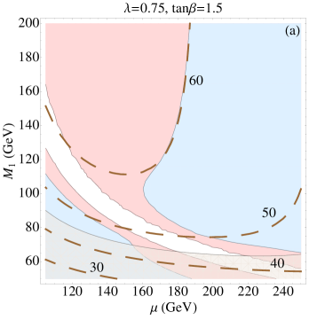
Refer to caption
Refer to caption
Figure 7: The well-tempered scenario at low tanβ𝛽\tan\beta, with χ~10subscriptsuperscript~𝜒01\widetilde{\chi}^{0}_{1} an admixture of bino, Higgsino and singlino. In (a), λ=0.75,tanβ=1.5formulae-sequence𝜆0.75𝛽1.5\lambda=0.75,~{}\tan\beta=1.5 and in (b), λ=0.9,tanβ=2.5formulae-sequence𝜆0.9𝛽2.5\lambda=0.9,~{}\tan\beta=2.5. The heavy Higgs states are decoupled at MA=5subscript𝑀𝐴5M_{A}=5 TeV. This choice of parameters fixes mh125similar-tosubscript𝑚125m_{h}\sim 125 GeV. Regions shaded red are excluded by LUX at 90%percent\% C.L., blue by hχ~10χ~10subscriptsuperscript~𝜒01subscriptsuperscript~𝜒01h\rightarrow\widetilde{\chi}^{0}_{1}~{}\widetilde{\chi}^{0}_{1} bounds and gray by Zχ~10χ~10𝑍subscriptsuperscript~𝜒01subscriptsuperscript~𝜒01Z\rightarrow\widetilde{\chi}^{0}_{1}~{}\widetilde{\chi}^{0}_{1} bounds. These constraints leave a small patch of parameter space that are still viable, the “blind spots”. The dashed lines are contours of Mχ~10subscript𝑀subscriptsuperscript~𝜒01M_{\tilde{\chi}^{0}_{1}} in GeV. More details are presented in the text.

In the limit where μμeff,M1much-less-thansuperscript𝜇subscript𝜇effsubscript𝑀1\mu^{\prime}\ll\mu_{\text{eff}},~{}M_{1}, precision electroweak contraints can be evaded by raising μeffsubscript𝜇eff\mu_{\text{eff}}, thereby decoupling the Higgsinos. However, raising μeffsubscript𝜇eff\mu_{\text{eff}} or tanβ𝛽\tan\beta suppresses the mass χ~10subscriptsuperscript~𝜒01\widetilde{\chi}^{0}_{1} as

Mχ~10μ+λ2v2μeffs2β/(μeff2+λ2v2)subscript𝑀subscriptsuperscript~𝜒01superscript𝜇superscript𝜆2superscript𝑣2subscript𝜇effsubscript𝑠2𝛽superscriptsubscript𝜇eff2superscript𝜆2superscript𝑣2\displaystyle M_{\tilde{\chi}^{0}_{1}}\approx\mu^{\prime}+\lambda^{2}v^{2}\mu_{\text{eff}}s_{2\beta}/(\mu_{\text{eff}}^{2}+\lambda^{2}v^{2}) (55)

for large M1subscript𝑀1M_{1} and M2subscript𝑀2M_{2}. As Mχ~10MZ/2subscript𝑀subscriptsuperscript~𝜒01subscript𝑀𝑍2M_{\tilde{\chi}^{0}_{1}}\leq M_{Z}/2 for a large region of parameters in this scenario, the invisible width of the Z𝑍Z boson is an important constraint. Consequently, to find a viable region of parameter space, we require μeffλvsimilar-tosubscript𝜇eff𝜆𝑣\mu_{\text{eff}}\sim\lambda v and small tanβ𝛽\tan\beta. In this region, ghχχsubscript𝑔𝜒𝜒g_{h\chi\chi} is supppressed when χ~10subscriptsuperscript~𝜒01\widetilde{\chi}^{0}_{1} is an admixture of B~~𝐵\widetilde{B}, ψ~u0subscriptsuperscript~𝜓0𝑢\widetilde{\psi}^{0}_{u}, and ψ~s0subscriptsuperscript~𝜓0𝑠\widetilde{\psi}^{0}_{s} such that they lead to “blind spots” in parameter space [42] – regions that are compatible with current experiment. For illustration, we have consistently set μ=0superscript𝜇0\mu^{\prime}=0 in this section.

We illustrate these blind spots in Fig. 7, which shows constraints on the LSP in the M1μeffsubscript𝑀1subscript𝜇effM_{1}-\mu_{\text{eff}} plane. Fig. 7(a) corresponds to tanβ=1.5𝛽1.5\tan\beta=1.5 and Fig. 7(b) to tanβ=2.5𝛽2.5\tan\beta=2.5. To fix mh125similar-tosubscript𝑚125m_{h}\sim 125 GeV, we take λ=0.75𝜆0.75\lambda=0.75 and λ=0.9𝜆0.9\lambda=0.9 respectively and decouple the heavy Higgses with MA=5subscript𝑀𝐴5M_{A}=5 TeV. At these values of λ𝜆\lambda, tanβ𝛽\tan\beta and MAsubscript𝑀𝐴M_{A} the Higgs mass is mainly set by the tree-level values as the loop level corrections are small. The regions shaded red are excluded by LUX at 90% C.L. Regions shaded blue are excluded by the latest limit on the invisible decay of the Higgs, ..(hχ~10χ~10)<0.44formulae-sequencesubscriptsuperscript~𝜒01subscriptsuperscript~𝜒010.44\mathcal{B.R.}(h\rightarrow\widetilde{\chi}^{0}_{1}\widetilde{\chi}^{0}_{1})<0.44 [57, 58]. The gray region is excluded by limits from the invisible decay of the Z𝑍Z. The dashed curves represent contours of Mχ~10subscript𝑀subscriptsuperscript~𝜒01M_{\tilde{\chi}^{0}_{1}} in GeV. This range of parameters is cosmologically viable with Ωχh2<0.12subscriptΩ𝜒superscript20.12\Omega_{\chi}h^{2}<0.12, where the dominant primordial annihilation of χ~10subscriptsuperscript~𝜒01\widetilde{\chi}^{0}_{1} is through an s𝑠s-channel Z𝑍Z.

A comparison across the plots informs us that an increase in tanβ𝛽\tan\beta strengthens the constraints from Z,hχ~10χ~10𝑍subscriptsuperscript~𝜒01subscriptsuperscript~𝜒01Z,h\rightarrow\widetilde{\chi}^{0}_{1}\widetilde{\chi}^{0}_{1}, which is due to the decrease in Mχ~10subscript𝑀subscriptsuperscript~𝜒01M_{\tilde{\chi}^{0}_{1}}, as discussed earlier. We also notice that the LUX constraints are consistently stronger than hχ~10χ~10subscriptsuperscript~𝜒01subscriptsuperscript~𝜒01h\rightarrow\widetilde{\chi}^{0}_{1}\widetilde{\chi}^{0}_{1} bounds. Therefore, the blind spots (unshaded regions) are determined in this case by limits from LUX and invisible Z𝑍Z decays alone. As mentioned in Sec. 2.3, larger values of λ𝜆\lambda contribute more to Tχsubscript𝑇𝜒T_{\chi}. For Fig. 7(a) and Fig. 7(b), Tχ<0.02subscript𝑇𝜒0.02T_{\chi}<0.02 (completely safe) and Tχ<0.11subscript𝑇𝜒0.11T_{\chi}<0.11 (marginally safe) in the blind spots. Also, using NMSSMTools 4.5.1 we find that Ωχh20.01similar-tosubscriptΩ𝜒superscript20.01\Omega_{\chi}h^{2}\sim 0.01 in the blind spots. Therefore, the well-tempered neutralino here can only make up a small fraction of the observed relic density.

3.4 Future prospects

In this region (large tanβ𝛽\tan\beta with μλvμeffsimilar-tosuperscript𝜇𝜆𝑣similar-tosubscript𝜇eff\mu^{\prime}\sim\lambda v\sim\mu_{\text{eff}}), the non-standard Higgs scalars are heavy with MAsubscript𝑀𝐴M_{A} between 48TeV48TeV4-8~{}\text{TeV}. Therefore the doublet-singlet mixing in the Higgs sector is very small leading to a  1%percent\% deviation in the Higgs signal strengths from the SM. Such deviations are much below the sensitivity of the LHC at present and future runs, and can only be tested at a future “Higgs factory”. However, the large tanβ𝛽\tan\beta scenarios can be probed by future dark matter direct detection experiments. In particular, the projected reach of the XENON1T experiment [36] corresponds to σSI10471046cm2subscript𝜎SIsuperscript1047superscript1046superscriptcm2\sigma_{\rm SI}\approx 10^{-47}-10^{-46}~{}{\rm cm}^{2} for dark matter masses between 505050 GeV and 500500500 GeV. Since the DM-nucleon scattering cross-sections for the large tanβ𝛽\tan\beta scenarios in Fig. 6 vary from 10461045cm2similar-toabsentsuperscript1046superscript1045superscriptcm2\sim 10^{-46}-10^{-45}~{}{\rm cm}^{2}, these regions can be probed at the XENON1T experiment. Unlike the large μ,tanβsuperscript𝜇𝛽\mu^{\prime},\tan\beta scenarios, XENON1T will only be able to probe some of the allowed regions of the well-tempered scenario because ghχχsubscript𝑔𝜒𝜒g_{h\chi\chi} in can be suppressed.

4 Conclusions

In this article we have investigated the viability of regions of large tanβ𝛽\tan\beta in the framework of Fat Higgs/λ𝜆\lambda-SUSY models. In the “toy” model we constructed we showed that the singlet cubic term is suppressed while the the tadpole and singlino mass parameter terms were allowed. Within this framework we showed that there are regions of large tanβ𝛽\tan\beta that are phenomenologically viable.

In particular, we computed the one-loop effective potential and showed that the tanβ𝛽\tan\beta-independent contributions to the Higgs quartic are crucial in raising the Higgs mass to the observed value of 125 GeV. We have also shown that non-standard Higgs bosons of the same mass as the stops will give comparable contributions to the Higgs quartic when λ3ytsimilar-to-or-equals𝜆3subscript𝑦𝑡\lambda\simeq\sqrt{3}y_{t}. In the region of degenerate non-standard Higgs boson masses the corrections are larger than those estimated in Ref. [35, 43]. This discrepancy is purely due to the assumptions made in Ref. [35, 43] that lead to a split spectrum of heavy CP-even and CP-odd scalars.

Furthermore, we pointed out that contributions of the neutralinos and charginos to electroweak precison observables are small even for large tanβ𝛽\tan\beta when μeff500similar-to-or-equalssubscript𝜇eff500\mu_{\rm eff}\simeq 500 GeV and μ>100superscript𝜇similar-to100\mu^{\prime}\begin{array}[]{c}\sim\vspace{-21pt}\\ >\end{array}100 GeV. Such large values of μeffsubscript𝜇eff\mu_{\rm eff} make this region of Fat Higgs/λ𝜆\lambda-SUSY parameter space slightly more unnatural than the low tanβ𝛽\tan\beta region considered in Ref. [22, 23, 24, 25, 26, 27, 28, 29, 30, 31, 32, 33, 34]. Additionally, this scenario corresponds to the decoupling limit where the mixing between the heavy Higgs states and the SM-like Higgs is suppressed. Consequently, SM-like Higgs decay properties are with 1% of their corresponding Standard Model values. Detecting this scenario at the LHC, therefore, will be challenging.

We also found regions of large tanβ𝛽\tan\beta in Fat Higgs/λ𝜆\lambda-SUSY models that satisfy all the above constraints and provide a viable dark matter candidate. For large μsuperscript𝜇\mu^{\prime} and tanβ𝛽\tan\beta we showed that four possible viable parametric scenarios exist. The dark matter in these scenarios could be either most singlino or bino and, depending on their mass, could generate the observed relic abundance through resonant annihilation or co-annihilation. In each of these scenarios, direct detection cross-section can be probed at the XENON1T experiment. Another possibility is that of a well-tempered neutralino. This scenario typically occurs at low values of tanβ𝛽\tan\beta and λ< 1superscriptsimilar-to𝜆1\lambda\>\raisebox{-2.15277pt}{$\stackrel{{\scriptstyle\textstyle<}}{{\sim}}$}\>1, where the lightest neutralino’s Higgsino, bino and singlino fractions are such that its coupling to the Higgs boson is suppressed. The XENON1T experiment may not be able to completely probe this scenario.

Acknowledgments

We are grateful to Kaustubh Agashe, Spencer Chang, Graham Kribs and Carlos Wagner for helpful discussions, and particularly SC and GK for reading our manuscript. NR thanks Notre Dame University, Michigan State University and University of Maryland for hospitality, where part of this work was completed. Our work at University of Oregon was supported in part by the US Department of Energy under contract number DE-SC0011640.

Appendix A Decoupling behavior at one-loop level

We need to use the tadpoles at the one-loop level to solved for the one-loop corrected soft squared mass parameters. Extending Eq. (26) to one-loop order leads to the system of three equations,

Ti=VHiggsϕisubscript𝑇𝑖subscript𝑉Higgssubscriptitalic-ϕ𝑖\displaystyle T_{i}=\frac{\partial V_{\rm Higgs}}{\partial\phi_{i}} =\displaystyle= VHiggstreeϕi|{vk}+ΔVϕi|{vk}=Titree+ΔTi=0,i=1,2,3.formulae-sequenceevaluated-atsubscriptsuperscript𝑉treeHiggssubscriptitalic-ϕ𝑖subscript𝑣𝑘evaluated-atΔ𝑉subscriptitalic-ϕ𝑖subscript𝑣𝑘subscriptsuperscript𝑇tree𝑖Δsubscript𝑇𝑖0𝑖123\displaystyle\left.\frac{\partial V^{\rm tree}_{\rm Higgs}}{\partial\phi_{i}}\right|_{\{v_{k}\}}+\left.\frac{\partial\Delta V}{\partial\phi_{i}}\right|_{\{v_{k}\}}=T^{\rm tree}_{i}+\Delta T_{i}=0,\ \ \ \ \ \ \ \ i=1,2,3. (56)

We again can try to solve for the soft masses mHu2,mHd2subscriptsuperscript𝑚2subscript𝐻𝑢subscriptsuperscript𝑚2subscript𝐻𝑑m^{2}_{H_{u}},m^{2}_{H_{d}} and mS2subscriptsuperscript𝑚2𝑆m^{2}_{S} in terms of the Higgs VEVs. Note that while each Titreesubscriptsuperscript𝑇tree𝑖T^{\rm tree}_{i}, as given in Eq. (26), contains only its corresponding soft mass mHi2subscriptsuperscript𝑚2subscript𝐻𝑖m^{2}_{H_{i}}, ΔTiΔsubscript𝑇𝑖\Delta T_{i} in general contain all three soft mass terms. Although obtaining the solutions to such a system of equations maybe straightforward, the computation could become complicated when we expand the full potential around the true electroweak symmetry breaking minimum. We can avoid this difficulty by solving Eq. (56) iteratively. We first solve for the tree level soft mass squared parameters (mHu02)0,(mHd02)0,(mS2)0superscriptsuperscriptsubscript𝑚superscriptsubscript𝐻𝑢020superscriptsuperscriptsubscript𝑚superscriptsubscript𝐻𝑑020superscriptsuperscriptsubscript𝑚𝑆20\left(m_{H_{u}^{0}}^{2}\right)^{0},\left(m_{H_{d}^{0}}^{2}\right)^{0},\left(m_{S}^{2}\right)^{0} using Eq. (26) and then substitute them into ΔTiΔsubscript𝑇𝑖\Delta T_{i}. This approximation linearizes Eq. (56) which leads to the one-loop corrected soft mass squared parameters solution

mi2=(mi2)0116π2j=D,SMA,j2vibj0ϕi|vi+superscriptsubscript𝑚𝑖2superscriptsuperscriptsubscript𝑚𝑖20evaluated-at116superscript𝜋2subscript𝑗𝐷𝑆subscriptsuperscript𝑀2𝐴𝑗subscript𝑣𝑖superscriptsubscript𝑏𝑗0subscriptitalic-ϕ𝑖subscript𝑣𝑖\displaystyle m_{i}^{2}=\left(m_{i}^{2}\right)^{0}-\frac{1}{16\pi^{2}}\sum_{j=D,S}\frac{M^{2}_{A,j}}{v_{i}}\left.\frac{\partial b_{j}^{0}}{\partial\phi_{i}}\right|_{v_{i}}+... (57)

where (mi2)0superscriptsuperscriptsubscript𝑚𝑖20\left(m_{i}^{2}\right)^{0} is the tree-level solutions of Eq. (26), bj0=bj((mi2)0)subscriptsuperscript𝑏0𝑗subscript𝑏𝑗superscriptsubscriptsuperscript𝑚2𝑖0b^{0}_{j}=b_{j}\left((m^{2}_{i})^{0}\right), vi=(vu,vd,s)subscript𝑣𝑖subscript𝑣𝑢subscript𝑣𝑑𝑠v_{i}=(v_{u},v_{d},s), i=(Hu0,Hd0,S)𝑖superscriptsubscript𝐻𝑢0superscriptsubscript𝐻𝑑0𝑆i=(H_{u}^{0},H_{d}^{0},S) and ϕi=(Hu0,Hd0,S)subscriptitalic-ϕ𝑖superscriptsubscript𝐻𝑢0superscriptsubscript𝐻𝑑0𝑆\phi_{i}=(H_{u}^{0},H_{d}^{0},S). Substituting these solutions into the total potential and expanding it about the electroweak symmetry breaking minimum we observe that corrections to the CP-even Higgs mass matrix takes the form

(ΔMH02)ab=116π2i=D,S(bi02ϕaϕb|{va}12vabi0ϕa|{va}δab)MA,i2+,superscriptΔsuperscriptsubscript𝑀superscript𝐻02𝑎𝑏116superscript𝜋2subscript𝑖𝐷𝑆evaluated-atsuperscriptsubscriptsuperscript𝑏0𝑖2subscriptitalic-ϕ𝑎subscriptitalic-ϕ𝑏subscript𝑣𝑎evaluated-at12subscript𝑣𝑎subscriptsuperscript𝑏0𝑖subscriptitalic-ϕ𝑎subscript𝑣𝑎subscript𝛿𝑎𝑏superscriptsubscript𝑀𝐴𝑖2\displaystyle\left(\Delta M_{H^{0}}^{2}\right)^{ab}=\frac{1}{16\pi^{2}}\sum_{i=D,S}\left(\left.\frac{\partial{b^{0}_{i}}^{2}}{\partial\phi_{a}\partial\phi_{b}}\right|_{\{v_{a}\}}-\left.\frac{1}{2v_{a}}\frac{\partial b^{0}_{i}}{\partial\phi_{a}}\right|_{\{v_{a}\}}\delta_{ab}\right)M_{A,i}^{2}+..., (58)

By the symmetries of the model, the only field dependences at quadratic order in bi0subscriptsuperscript𝑏0𝑖b^{0}_{i} are hu2,hd2,huhdsubscriptsuperscript2𝑢subscriptsuperscript2𝑑subscript𝑢subscript𝑑h^{2}_{u},h^{2}_{d},h_{u}h_{d} and hs2subscriptsuperscript2𝑠h^{2}_{s}. Thus Eq. (58) suggests that the coefficient of MAS2subscriptsuperscript𝑀2subscript𝐴𝑆M^{2}_{A_{S}} in the self-energy corrections vanishes and that of MAD2subscriptsuperscript𝑀2subscript𝐴𝐷M^{2}_{A_{D}} will be proportional to

v2sβcβ(cβ2sβcβ0sβcβsβ20000).superscript𝑣2subscript𝑠𝛽subscript𝑐𝛽subscriptsuperscript𝑐2𝛽subscript𝑠𝛽subscript𝑐𝛽0subscript𝑠𝛽subscript𝑐𝛽subscriptsuperscript𝑠2𝛽0000\displaystyle-\frac{v^{2}}{s_{\beta}c_{\beta}}\left(\begin{array}[]{ccc}c^{2}_{\beta}&-s_{\beta}c_{\beta}&0\\ -s_{\beta}c_{\beta}&s^{2}_{\beta}&0\\ 0&0&0\end{array}\right). (62)

When these correction are rotated into the basis defined in Eq. (30) we see that the (2,2)22(2,2) element is the only non-zero element. Therefore the decoupling is manifest even at the one-loop level.

Appendix B Effective potential derivation

In this section we apply the procedure outlined in Sec. 2.2 to the computation of one-loop radiative corrections from the Higgs sector. First, we deal with degenerate pseudoscalars, so that all the one-loop corrections come from a single heavy scale. We will call this Case (A). Next, in Case (B), we inspect the effect of splitting the pseudoscalar masses on the one-loop corrections, where they now come from two heavy scales. For simplicity, the soft terms Aλ,Aκ,μ,m3,mSsubscript𝐴𝜆subscript𝐴𝜅superscript𝜇subscript𝑚3superscriptsubscript𝑚𝑆A_{\lambda},A_{\kappa},\mu^{\prime},m_{3},m_{S}^{\prime} are taken to vanish in this case.

(A) Degenerate pseudoscalars

From the CP-odd mass matrix in Eq. (28), we impose the necessary and sufficient condition for mass degeneracy in the pseudoscalars given by (MA2)12=0,(MA2)11=(MA2)22=MA2formulae-sequencesubscriptsubscriptsuperscript𝑀2𝐴120subscriptsubscriptsuperscript𝑀2𝐴11subscriptsubscriptsuperscript𝑀2𝐴22subscriptsuperscript𝑀2𝐴\left(M^{2}_{A}\right)_{12}=0,\left(M^{2}_{A}\right)_{11}=\left(M^{2}_{A}\right)_{22}=M^{2}_{A}, to obtain

μsuperscript𝜇\displaystyle\mu^{\prime} =\displaystyle= Aλ,subscript𝐴𝜆\displaystyle A_{\lambda},
ξFsubscript𝜉𝐹\displaystyle\xi_{F} =\displaystyle= (MA2sβcβm32)/λ2Aλs,subscriptsuperscript𝑀2𝐴subscript𝑠𝛽subscript𝑐𝛽subscriptsuperscript𝑚23𝜆2subscript𝐴𝜆𝑠\displaystyle(M^{2}_{A}s_{\beta}c_{\beta}-m^{2}_{3})/\lambda-2A_{\lambda}s,
ξSsubscript𝜉𝑆\displaystyle\xi_{S} =\displaystyle= MA2sAλ(MA2sβcβm32λv2s2β)/λsubscriptsuperscript𝑀2𝐴𝑠subscript𝐴𝜆subscriptsuperscript𝑀2𝐴subscript𝑠𝛽subscript𝑐𝛽subscriptsuperscript𝑚23𝜆superscript𝑣2subscript𝑠2𝛽𝜆\displaystyle-M^{2}_{A}s-A_{\lambda}(M^{2}_{A}s_{\beta}c_{\beta}-m^{2}_{3}-\lambda v^{2}s_{2\beta})/\lambda (63)

Respecting this condition, the field-dependent mass matrix for the charged sector is

M11±2superscriptsuperscriptsubscript𝑀11plus-or-minus2\displaystyle{M_{11}^{\pm}}^{2} =\displaystyle= mHu2+λ2hs2+g24(hu2hd2)+g222hd2,superscriptsubscript𝑚subscript𝐻𝑢2superscript𝜆2superscriptsubscript𝑠2superscript𝑔24superscriptsubscript𝑢2superscriptsubscript𝑑2superscriptsubscript𝑔222superscriptsubscript𝑑2\displaystyle m_{H_{u}}^{2}+\lambda^{2}h_{s}^{2}+\frac{g^{2}}{4}(h_{u}^{2}-h_{d}^{2})+\frac{g_{2}^{2}}{2}h_{d}^{2},
M12±2superscriptsuperscriptsubscript𝑀12plus-or-minus2\displaystyle{M_{12}^{\pm}}^{2} =\displaystyle= (g222λ2)huhd+2λAλ(hss)+MA2sβcβ,superscriptsubscript𝑔222superscript𝜆2subscript𝑢subscript𝑑2𝜆subscript𝐴𝜆subscript𝑠𝑠subscriptsuperscript𝑀2𝐴subscript𝑠𝛽subscript𝑐𝛽\displaystyle(\frac{g_{2}^{2}}{2}-\lambda^{2})h_{u}h_{d}+2\lambda A_{\lambda}(h_{s}-s)+M^{2}_{A}s_{\beta}c_{\beta},
M22±2superscriptsuperscriptsubscript𝑀22plus-or-minus2\displaystyle{M_{22}^{\pm}}^{2} =\displaystyle= mHd2+λ2hs2g24(hu2hd2)+g222hu2,superscriptsubscript𝑚subscript𝐻𝑑2superscript𝜆2superscriptsubscript𝑠2superscript𝑔24superscriptsubscript𝑢2superscriptsubscript𝑑2superscriptsubscript𝑔222superscriptsubscript𝑢2\displaystyle m_{H_{d}}^{2}+\lambda^{2}h_{s}^{2}-\frac{g^{2}}{4}(h_{u}^{2}-h_{d}^{2})+\frac{g_{2}^{2}}{2}h_{u}^{2}, (64)

for the CP-odd sector it is

M11P2superscriptsuperscriptsubscript𝑀11𝑃2\displaystyle{M_{11}^{P}}^{2} =\displaystyle= mHu2+λ2(hd2+hs2)+g24(hu2hd2),superscriptsubscript𝑚subscript𝐻𝑢2superscript𝜆2superscriptsubscript𝑑2superscriptsubscript𝑠2superscript𝑔24superscriptsubscript𝑢2superscriptsubscript𝑑2\displaystyle m_{H_{u}}^{2}+\lambda^{2}(h_{d}^{2}+h_{s}^{2})+\frac{g^{2}}{4}(h_{u}^{2}-h_{d}^{2}),
M12P2superscriptsuperscriptsubscript𝑀12𝑃2\displaystyle{M_{12}^{P}}^{2} =\displaystyle= 2λAλ(hss)+MA2sβcβ,2𝜆subscript𝐴𝜆subscript𝑠𝑠subscriptsuperscript𝑀2𝐴subscript𝑠𝛽subscript𝑐𝛽\displaystyle 2\lambda A_{\lambda}(h_{s}-s)+M^{2}_{A}s_{\beta}c_{\beta},
M22P2superscriptsuperscriptsubscript𝑀22𝑃2\displaystyle{M_{22}^{P}}^{2} =\displaystyle= mHd2+λ2(hu2+hs2)g24(hu2hd2),superscriptsubscript𝑚subscript𝐻𝑑2superscript𝜆2superscriptsubscript𝑢2superscriptsubscript𝑠2superscript𝑔24superscriptsubscript𝑢2superscriptsubscript𝑑2\displaystyle m_{H_{d}}^{2}+\lambda^{2}(h_{u}^{2}+h_{s}^{2})-\frac{g^{2}}{4}(h_{u}^{2}-h_{d}^{2}),
M13P2superscriptsuperscriptsubscript𝑀13𝑃2\displaystyle{M_{13}^{P}}^{2} =\displaystyle= 0,0\displaystyle 0,
M23P2superscriptsuperscriptsubscript𝑀23𝑃2\displaystyle{M_{23}^{P}}^{2} =\displaystyle= 0,0\displaystyle 0,
M33P2superscriptsuperscriptsubscript𝑀33𝑃2\displaystyle{M_{33}^{P}}^{2} =\displaystyle= mS2+λ2(hu2+hd2)+Aλ2ms2,superscriptsubscript𝑚𝑆2superscript𝜆2superscriptsubscript𝑢2superscriptsubscript𝑑2subscriptsuperscript𝐴2𝜆superscriptsubscriptsuperscript𝑚𝑠2\displaystyle m_{S}^{2}+\lambda^{2}(h_{u}^{2}+h_{d}^{2})+A^{2}_{\lambda}-{m^{\prime}_{s}}^{2},

and for the CP-even sector it is

M11S2superscriptsuperscriptsubscript𝑀11𝑆2\displaystyle{M_{11}^{S}}^{2} =\displaystyle= mHu2+λ2(hd2+hs2)+g24(3hu2hd2),superscriptsubscript𝑚subscript𝐻𝑢2superscript𝜆2superscriptsubscript𝑑2superscriptsubscript𝑠2superscript𝑔243superscriptsubscript𝑢2superscriptsubscript𝑑2\displaystyle m_{H_{u}}^{2}+\lambda^{2}(h_{d}^{2}+h_{s}^{2})+\frac{g^{2}}{4}(3h_{u}^{2}-h_{d}^{2}),
M12S2superscriptsuperscriptsubscript𝑀12𝑆2\displaystyle{M_{12}^{S}}^{2} =\displaystyle= (2λ2g22)huhd2λAλ(hss)+MA2sβcβ,2superscript𝜆2superscript𝑔22subscript𝑢subscript𝑑2𝜆subscript𝐴𝜆subscript𝑠𝑠subscriptsuperscript𝑀2𝐴subscript𝑠𝛽subscript𝑐𝛽\displaystyle(2\lambda^{2}-\frac{g^{2}}{2})h_{u}h_{d}-2\lambda A_{\lambda}(h_{s}-s)+M^{2}_{A}s_{\beta}c_{\beta},
M22S2superscriptsuperscriptsubscript𝑀22𝑆2\displaystyle{M_{22}^{S}}^{2} =\displaystyle= mHd2+λ2(hu2+hs2)g24(hu23hd2),superscriptsubscript𝑚subscript𝐻𝑑2superscript𝜆2superscriptsubscript𝑢2superscriptsubscript𝑠2superscript𝑔24superscriptsubscript𝑢23superscriptsubscript𝑑2\displaystyle m_{H_{d}}^{2}+\lambda^{2}(h_{u}^{2}+h_{s}^{2})-\frac{g^{2}}{4}(h_{u}^{2}-3h_{d}^{2}),
M13S2superscriptsuperscriptsubscript𝑀13𝑆2\displaystyle{M_{13}^{S}}^{2} =\displaystyle= 2λ2(huhsAλhd),2superscript𝜆2subscript𝑢subscript𝑠subscript𝐴𝜆subscript𝑑\displaystyle 2\lambda^{2}(h_{u}h_{s}-A_{\lambda}h_{d}),
M23S2superscriptsuperscriptsubscript𝑀23𝑆2\displaystyle{M_{23}^{S}}^{2} =\displaystyle= 2λ2(hdhsAλhu),2superscript𝜆2subscript𝑑subscript𝑠subscript𝐴𝜆subscript𝑢\displaystyle 2\lambda^{2}(h_{d}h_{s}-A_{\lambda}h_{u}),
M33S2superscriptsuperscriptsubscript𝑀33𝑆2\displaystyle{M_{33}^{S}}^{2} =\displaystyle= mS2+λ2(hu2+hd2)+Aλ2+ms2subscriptsuperscript𝑚2𝑆superscript𝜆2superscriptsubscript𝑢2superscriptsubscript𝑑2subscriptsuperscript𝐴2𝜆superscriptsubscriptsuperscript𝑚𝑠2\displaystyle m^{2}_{S}+\lambda^{2}(h_{u}^{2}+h_{d}^{2})+A^{2}_{\lambda}+{m^{\prime}_{s}}^{2}

The eigenvalues of the charged matrix are given by M1,2±2=12(TrcTrc24Detc)superscriptsuperscriptsubscript𝑀12plus-or-minus212minus-or-plussubscriptTr𝑐superscriptsubscriptTr𝑐24subscriptDet𝑐{M_{1,2}^{\pm}}^{2}=\frac{1}{2}(\text{Tr}_{c}\mp\sqrt{\text{Tr}_{c}^{2}-4\text{Det}_{c}}), where Trc=M11±2+M22±2subscriptTr𝑐superscriptsuperscriptsubscript𝑀11plus-or-minus2superscriptsuperscriptsubscript𝑀22plus-or-minus2\text{Tr}_{c}={M_{11}^{\pm}}^{2}+{M_{22}^{\pm}}^{2} and Detc=M11±2M22±2M12±2M21±2subscriptDet𝑐superscriptsuperscriptsubscript𝑀11plus-or-minus2superscriptsuperscriptsubscript𝑀22plus-or-minus2superscriptsuperscriptsubscript𝑀12plus-or-minus2superscriptsuperscriptsubscript𝑀21plus-or-minus2\text{Det}_{c}={M_{11}^{\pm}}^{2}{M_{22}^{\pm}}^{2}-{M_{12}^{\pm}}^{2}{M_{21}^{\pm}}^{2}. We only include the contribution from the heavier eigenstate corresponding to M2±2superscriptsuperscriptsubscript𝑀2plus-or-minus2{M_{2}^{\pm}}^{2}. Note that when we take the supertrace in the charged higgs sector, we obtain a multiplicative factor of 2 since each charged higgs state comprises of two real physical states. In other words, the supertrace is here taken over the full 4×4444\times 4 squared-mass matrix and not the 2×2222\times 2 version that is usually written down for brevity.

The eigenvalues of the CP-odd matrix are obtained in a straightforward manner, since the upper left 2×2222\times 2 block is decoupled from M33P2superscriptsuperscriptsubscript𝑀33𝑃2{M_{33}^{P}}^{2}. The squared eigenmasses are obtained as M1,p2=12(TrpTrp24Detp),M2,p2=12(Trp+Trp24Detp)formulae-sequencesubscriptsuperscript𝑀21𝑝12subscriptTr𝑝superscriptsubscriptTr𝑝24subscriptDet𝑝subscriptsuperscript𝑀22𝑝12subscriptTr𝑝superscriptsubscriptTr𝑝24subscriptDet𝑝M^{2}_{1,p}=\frac{1}{2}(\text{Tr}_{p}-\sqrt{\text{Tr}_{p}^{2}-4\text{Det}_{p}}),M^{2}_{2,p}=\frac{1}{2}(\text{Tr}_{p}+\sqrt{\text{Tr}_{p}^{2}-4\text{Det}_{p}}) and M3,p2=M332subscriptsuperscript𝑀23𝑝subscriptsuperscript𝑀233M^{2}_{3,p}=M^{2}_{33}, where Trp=M11P2+M22P2subscriptTr𝑝superscriptsubscriptsuperscript𝑀𝑃112superscriptsubscriptsuperscript𝑀𝑃222\text{Tr}_{p}={M^{P}_{11}}^{2}+{M^{P}_{22}}^{2} and Detp=M11P2M22P2M12P2M21P2subscriptDet𝑝superscriptsubscriptsuperscript𝑀𝑃112superscriptsubscriptsuperscript𝑀𝑃222superscriptsubscriptsuperscript𝑀𝑃122superscriptsubscriptsuperscript𝑀𝑃212\text{Det}_{p}={M^{P}_{11}}^{2}{M^{P}_{22}}^{2}-{M^{P}_{12}}^{2}{M^{P}_{21}}^{2}.

Obtaining the CP-even eigenvalues is non-trivial since we need to deal with a rank 3 matrix. However, we can take advantage of the degeneracy of the CP-odd scalars by employing the following simplifying trick.

First, consider the characteristic equation of the CP-even matrix, written as

α3x3+α2x2+α1x+α0=0,subscript𝛼3superscript𝑥3subscript𝛼2superscript𝑥2subscript𝛼1𝑥subscript𝛼00\displaystyle\alpha_{3}x^{3}+\alpha_{2}x^{2}+\alpha_{1}x+\alpha_{0}=0,

whose solutions are the field-dependent eigenmasses Mi,s2subscriptsuperscript𝑀2𝑖𝑠M^{2}_{i,s}. The coefficients αisubscript𝛼𝑖\alpha_{i}, in terms of the matrix elements in Eq. (LABEL:eq:fielddep_massmat_cpeven), are

α3subscript𝛼3\displaystyle\alpha_{3} =\displaystyle= 1,1\displaystyle 1,
α2subscript𝛼2\displaystyle\alpha_{2} =\displaystyle= (M11S2+M22S2+M33S2),superscriptsuperscriptsubscript𝑀11𝑆2superscriptsuperscriptsubscript𝑀22𝑆2superscriptsuperscriptsubscript𝑀33𝑆2\displaystyle-({M_{11}^{S}}^{2}+{M_{22}^{S}}^{2}+{M_{33}^{S}}^{2}),
α1subscript𝛼1\displaystyle\alpha_{1} =\displaystyle= M11S2M22S2+M22S2M33S2+M33S2M11S2M12S2M21S2M23S2M32S2M31S2M13S2,superscriptsuperscriptsubscript𝑀11𝑆2superscriptsuperscriptsubscript𝑀22𝑆2superscriptsuperscriptsubscript𝑀22𝑆2superscriptsuperscriptsubscript𝑀33𝑆2superscriptsuperscriptsubscript𝑀33𝑆2superscriptsuperscriptsubscript𝑀11𝑆2superscriptsuperscriptsubscript𝑀12𝑆2superscriptsuperscriptsubscript𝑀21𝑆2superscriptsuperscriptsubscript𝑀23𝑆2superscriptsuperscriptsubscript𝑀32𝑆2superscriptsuperscriptsubscript𝑀31𝑆2superscriptsuperscriptsubscript𝑀13𝑆2\displaystyle{M_{11}^{S}}^{2}{M_{22}^{S}}^{2}+{M_{22}^{S}}^{2}{M_{33}^{S}}^{2}+{M_{33}^{S}}^{2}{M_{11}^{S}}^{2}-{M_{12}^{S}}^{2}{M_{21}^{S}}^{2}-{M_{23}^{S}}^{2}{M_{32}^{S}}^{2}-{M_{31}^{S}}^{2}{M_{13}^{S}}^{2},
α0subscript𝛼0\displaystyle\alpha_{0} =\displaystyle= [M11S2(M22S2M33S2M23S2M32S2)M12S2(M21S2M33S2M23S2M31S2)\displaystyle-[{M_{11}^{S}}^{2}({M_{22}^{S}}^{2}{M_{33}^{S}}^{2}-{M_{23}^{S}}^{2}{M_{32}^{S}}^{2})-{M_{12}^{S}}^{2}({M_{21}^{S}}^{2}{M_{33}^{S}}^{2}-{M_{23}^{S}}^{2}{M_{31}^{S}}^{2}) (67)
+M13S2(M21S2M32S2M22S2M31S2)]\displaystyle~{}~{}+{M_{13}^{S}}^{2}({M_{21}^{S}}^{2}{M_{32}^{S}}^{2}-{M_{22}^{S}}^{2}{M_{31}^{S}}^{2})]

We also know, in terms of the eigenmasses, that

α2subscript𝛼2\displaystyle\alpha_{2} =\displaystyle= (M1,s2+M2,s2+M3,s2),subscriptsuperscript𝑀21𝑠subscriptsuperscript𝑀22𝑠subscriptsuperscript𝑀23𝑠\displaystyle-(M^{2}_{1,s}+M^{2}_{2,s}+M^{2}_{3,s}),
α1subscript𝛼1\displaystyle\alpha_{1} =\displaystyle= M1,s2M2,s2+M2,s2M3,s2+M3,s2M1,s2subscriptsuperscript𝑀21𝑠subscriptsuperscript𝑀22𝑠subscriptsuperscript𝑀22𝑠subscriptsuperscript𝑀23𝑠subscriptsuperscript𝑀23𝑠subscriptsuperscript𝑀21𝑠\displaystyle M^{2}_{1,s}M^{2}_{2,s}+M^{2}_{2,s}M^{2}_{3,s}+M^{2}_{3,s}M^{2}_{1,s} (68)

Now the CP-even sector contribution to the effective potential, from Eq. (32), is

ΔV164π2[(M2,s2)2+(M3,s2)2]log(MA2MZ2).164superscript𝜋2delimited-[]superscriptsubscriptsuperscript𝑀22𝑠2superscriptsubscriptsuperscript𝑀23𝑠2subscriptsuperscript𝑀2𝐴subscriptsuperscript𝑀2𝑍Δ𝑉\displaystyle\Delta V\supset\frac{1}{64\pi^{2}}[(M^{2}_{2,s})^{2}+(M^{2}_{3,s})^{2}]\log\left(\frac{M^{2}_{A}}{M^{2}_{Z}}\right). (69)

The quantity in brackets can be re-written using Eq. (68) as simply

(M2,s2)2+(M3,s2)2=α222α1(M1,s2)2superscriptsubscriptsuperscript𝑀22𝑠2superscriptsubscriptsuperscript𝑀23𝑠2subscriptsuperscript𝛼222subscript𝛼1superscriptsubscriptsuperscript𝑀21𝑠2\displaystyle(M^{2}_{2,s})^{2}+(M^{2}_{3,s})^{2}=\alpha^{2}_{2}-2\alpha_{1}-(M^{2}_{1,s})^{2} (70)

The coefficients α1subscript𝛼1\alpha_{1} and α2subscript𝛼2\alpha_{2} may be read off Eq. (67), while we may still have to determine M1,s2subscriptsuperscript𝑀21𝑠M^{2}_{1,s} analytically. This is, however, a simple task if we write M1,s2subscriptsuperscript𝑀21𝑠M^{2}_{1,s} as a power series in MA2::subscriptsuperscript𝑀2𝐴absentM^{2}_{A}:

M1,s2subscriptsuperscript𝑀21𝑠\displaystyle M^{2}_{1,s} =\displaystyle= b1+𝒪(1MA2)subscript𝑏1𝒪1subscriptsuperscript𝑀2𝐴\displaystyle b_{1}+\mathcal{O}\left(\frac{1}{M^{2}_{A}}\right)
(M1,s2)2absentsuperscriptsubscriptsuperscript𝑀21𝑠2\displaystyle\implies(M^{2}_{1,s})^{2} =\displaystyle= b12+𝒪(1MA2),subscriptsuperscript𝑏21𝒪1subscriptsuperscript𝑀2𝐴\displaystyle b^{2}_{1}+\mathcal{O}\left(\frac{1}{M^{2}_{A}}\right), (71)

where b1subscript𝑏1b_{1} is at most quadratic in the background fields. Putting Eqs. 70 and 71 into Eq. (69), we obtain the one-loop effective potential contribution simply as

ΔV164π2[α222α1b12]log(MA2MZ2),164superscript𝜋2delimited-[]subscriptsuperscript𝛼222subscript𝛼1subscriptsuperscript𝑏21subscriptsuperscript𝑀2𝐴subscriptsuperscript𝑀2𝑍Δ𝑉\displaystyle\Delta V\supset\frac{1}{64\pi^{2}}[\alpha^{2}_{2}-2\alpha_{1}-b^{2}_{1}]\log\left(\frac{M^{2}_{A}}{M^{2}_{Z}}\right), (72)

where we have discarded 𝒪(1/MA2)𝒪1subscriptsuperscript𝑀2𝐴\mathcal{O}(1/M^{2}_{A}) terms that are irrelevant in obtaining the required self-energy corrections.

After including all the one-loop corrections, the final expressions we obtain for the CP-even mass matrix are now as follows.

(M¯H2)11=MZ2sβ2+M¯A2cβ2+Π11;subscriptsubscriptsuperscript¯𝑀2𝐻11subscriptsuperscript𝑀2𝑍subscriptsuperscript𝑠2𝛽subscriptsuperscript¯𝑀2𝐴subscriptsuperscript𝑐2𝛽subscriptΠ11\displaystyle\left(\overline{M}^{2}_{H}\right)_{11}=M^{2}_{Z}s^{2}_{\beta}+\overline{M}^{2}_{A}c^{2}_{\beta}+\Pi_{11}; (M¯H2)12=(2λ2v2MZ2M¯A2)sβcβ+Π12;subscriptsubscriptsuperscript¯𝑀2𝐻122superscript𝜆2superscript𝑣2subscriptsuperscript𝑀2𝑍subscriptsuperscript¯𝑀2𝐴subscript𝑠𝛽subscript𝑐𝛽subscriptΠ12\displaystyle\left(\overline{M}^{2}_{H}\right)_{12}=(2\lambda^{2}v^{2}-M^{2}_{Z}-\overline{M}^{2}_{A})s_{\beta}c_{\beta}+\Pi_{12};
(M¯H2)22=MZ2cβ2+M¯A2+Π22;subscriptsubscriptsuperscript¯𝑀2𝐻22subscriptsuperscript𝑀2𝑍subscriptsuperscript𝑐2𝛽subscriptsuperscript¯𝑀2𝐴subscriptΠ22\displaystyle\left(\overline{M}^{2}_{H}\right)_{22}=M^{2}_{Z}c^{2}_{\beta}+\overline{M}^{2}_{A}+\Pi_{22}; (M¯H2)13=2λvμeffsβ+Π13;subscriptsubscriptsuperscript¯𝑀2𝐻132𝜆𝑣subscript𝜇effsubscript𝑠𝛽subscriptΠ13\displaystyle\left(\overline{M}^{2}_{H}\right)_{13}=2\lambda v\mu_{\text{eff}}s_{\beta}+\Pi_{13};
(M¯H2)23=2λvμeffcβ+Π23;subscriptsubscriptsuperscript¯𝑀2𝐻232𝜆𝑣subscript𝜇effsubscript𝑐𝛽subscriptΠ23\displaystyle\left(\overline{M}^{2}_{H}\right)_{23}=2\lambda v\mu_{\text{eff}}c_{\beta}+\Pi_{23}; (M¯H2)33=M¯A2+Π33,subscriptsubscriptsuperscript¯𝑀2𝐻33subscriptsuperscript¯𝑀2𝐴subscriptΠ33\displaystyle\left(\overline{M}^{2}_{H}\right)_{33}=\overline{M}^{2}_{A}+\Pi_{33},

where

M¯A2subscriptsuperscript¯𝑀2𝐴\displaystyle\overline{M}^{2}_{A} =\displaystyle= MA2(1+λ28π2log(MA2MZ2)),subscriptsuperscript𝑀2𝐴1superscript𝜆28superscript𝜋2subscriptsuperscript𝑀2𝐴subscriptsuperscript𝑀2𝑍\displaystyle M^{2}_{A}\left(1+\frac{\lambda^{2}}{8\pi^{2}}\log\left(\frac{M^{2}_{A}}{M^{2}_{Z}}\right)\right), (73)

and

Π11subscriptΠ11\displaystyle\Pi_{11} =\displaystyle= v2256π2[32λ4sβ2(2c2βs2β2)+2λ2g2(3c2β1)(3s2β2+2)\displaystyle\frac{v^{2}}{256\pi^{2}}[-32\lambda^{4}s_{\beta}^{2}(2c_{2\beta}-s_{2\beta}^{2})+2\lambda^{2}g^{2}(3c_{2\beta}-1)(3s_{2\beta}^{2}+2)
+g4(4cW4+4cW27s2β21c2β(4cW44cW2+5s2β2+3))superscript𝑔44superscriptsubscript𝑐𝑊44superscriptsubscript𝑐𝑊27superscriptsubscript𝑠2𝛽21subscript𝑐2𝛽4superscriptsubscript𝑐𝑊44superscriptsubscript𝑐𝑊25superscriptsubscript𝑠2𝛽23\displaystyle+g^{4}(4c_{W}^{4}+4c_{W}^{2}-7s_{2\beta}^{2}-1-c_{2\beta}(4c_{W}^{4}-4c_{W}^{2}+5s_{2\beta}^{2}+3))
+64λ2Aλμeffv2cotβ]log(MA2MZ2),\displaystyle+64\lambda^{2}\frac{A_{\lambda}\mu_{\text{eff}}}{v^{2}}\cot\beta]\log\left(\frac{M^{2}_{A}}{M^{2}_{Z}}\right),
Π12subscriptΠ12\displaystyle\Pi_{12} =\displaystyle= v2256π2[32λ4(s2β22)2λ2g2s2β(8cW215s2β2+14)\displaystyle\frac{v^{2}}{256\pi^{2}}[-32\lambda^{4}(s_{2\beta}^{2}-2)-2\lambda^{2}g^{2}s_{2\beta}(8c_{W}^{2}-15s_{2\beta}^{2}+14)
+g4s2β(4cW4+4cW27s2β2+3)superscript𝑔4subscript𝑠2𝛽4superscriptsubscript𝑐𝑊44superscriptsubscript𝑐𝑊27superscriptsubscript𝑠2𝛽23\displaystyle+g^{4}s_{2\beta}(4c_{W}^{4}+4c_{W}^{2}-7s_{2\beta}^{2}+3)
64λ2Aλμeffv2]log(MA2MZ2),\displaystyle-64\lambda^{2}\frac{A_{\lambda}\mu_{\text{eff}}}{v^{2}}]\log\left(\frac{M^{2}_{A}}{M^{2}_{Z}}\right),
Π22subscriptΠ22\displaystyle\Pi_{22} =\displaystyle= v2256π2[32λ4cβ2(2c2β+s2β2)2λ2g2(3c2β+1)(3s2β2+2)\displaystyle\frac{v^{2}}{256\pi^{2}}[32\lambda^{4}c_{\beta}^{2}(2c_{2\beta}+s_{2\beta}^{2})-2\lambda^{2}g^{2}(3c_{2\beta}+1)(3s_{2\beta}^{2}+2)
+g4(4cW44cW2+7s2β2+1+c2β(4cW44cW2+5s2β2+3))superscript𝑔44superscriptsubscript𝑐𝑊44superscriptsubscript𝑐𝑊27superscriptsubscript𝑠2𝛽21subscript𝑐2𝛽4superscriptsubscript𝑐𝑊44superscriptsubscript𝑐𝑊25superscriptsubscript𝑠2𝛽23\displaystyle+g^{4}(4c_{W}^{4}-4c_{W}^{2}+7s_{2\beta}^{2}+1+c_{2\beta}(4c_{W}^{4}-4c_{W}^{2}+5s_{2\beta}^{2}+3))
+64λ2Aλμeffv2tanβ]log(MA2MZ2),\displaystyle+64\lambda^{2}\frac{A_{\lambda}\mu_{\text{eff}}}{v^{2}}\tan\beta]\log\left(\frac{M^{2}_{A}}{M^{2}_{Z}}\right),
Π13subscriptΠ13\displaystyle\Pi_{13} =\displaystyle= vμeffμeff[12λ3sβ3+λg2sβ(3c2β+2cW2+1)\displaystyle\frac{v\mu_{\text{eff}}}{\mu_{\text{eff}}}[12\lambda^{3}s_{\beta}^{3}+\lambda g^{2}s_{\beta}(3c_{2\beta}+2c_{W}^{2}+1)
+λvAλcosβ32π2(λ2(13+3c4β)+g22(5+4cW26c2β+3c4β))]log(MA2MZ2),\displaystyle+\frac{\lambda vA_{\lambda}\cos\beta}{32\pi^{2}}\left(-\lambda^{2}(13+3c_{4\beta})+\frac{g^{2}}{2}(5+4c^{2}_{W}-6c_{2\beta}+3c_{4\beta})\right)]\log\left(\frac{M^{2}_{A}}{M^{2}_{Z}}\right),
Π23subscriptΠ23\displaystyle\Pi_{23} =\displaystyle= vμeffμeff[12λ3cβ3+λg2cβ(3c2β+2cW2+1))\displaystyle\frac{v\mu_{\text{eff}}}{\mu_{\text{eff}}}[12\lambda^{3}c_{\beta}^{3}+\lambda g^{2}c_{\beta}(-3c_{2\beta}+2c_{W}^{2}+1))
+λvAλsinβ32π2(λ2(13+3c4β)+g22(5+4cW2+6c2β+3c4β))]log(MA2MZ2),\displaystyle+\frac{\lambda vA_{\lambda}\sin\beta}{32\pi^{2}}\left(-\lambda^{2}(13+3c_{4\beta})+\frac{g^{2}}{2}(5+4c^{2}_{W}+6c_{2\beta}+3c_{4\beta})\right)]\log\left(\frac{M^{2}_{A}}{M^{2}_{Z}}\right),
Π33subscriptΠ33\displaystyle\Pi_{33} =\displaystyle= {4λ2μeff216π2+λAλ128π2[λ(16Aλ(4+c4β)\displaystyle\{\frac{4\lambda^{2}\mu_{\text{eff}}^{2}}{16\pi^{2}}+\frac{\lambda A_{\lambda}}{128\pi^{2}}[\lambda(16A_{\lambda}(4+c_{4\beta}) (74)
+λ(64s2+29v2)s2β+λv2s6β)+g2v2s2β(3+4cW2+c4β)]}log(MA2MZ2)\displaystyle+\lambda(64s^{2}+29v^{2})s_{2\beta}+\lambda v^{2}s_{6\beta})+g^{2}v^{2}s_{2\beta}(3+4c^{2}_{W}+c_{4\beta})]\}\log\left(\frac{M^{2}_{A}}{M^{2}_{Z}}\right)

If we set all NMSSM-specific parameters to zero in the above, we recover the MSSM limit presented in [60, 61, 62, 63]. The soft term Aλsubscript𝐴𝜆A_{\lambda} decouples at one-loop order and does not contribute to the SM Higgs quartic coupling, a property best seen in the basis of Eq. (30). The SM Higgs boson mass is then identified as

M¯hh2subscriptsuperscript¯𝑀2\displaystyle\overline{M}^{2}_{hh} =\displaystyle= λ2v2s2β2+MZ2c2β2+Πhh,superscript𝜆2superscript𝑣2subscriptsuperscript𝑠22𝛽subscriptsuperscript𝑀2𝑍subscriptsuperscript𝑐22𝛽subscriptΠ\displaystyle\lambda^{2}v^{2}s^{2}_{2\beta}+M^{2}_{Z}c^{2}_{2\beta}+\Pi_{hh},
ΠhhsubscriptΠ\displaystyle\Pi_{hh} =\displaystyle= v2512π2[4λ4(31+4c4β3c8β)+4λ2g2(94cW2+(4cW22)c4β+3c8β)\displaystyle\frac{v^{2}}{512\pi^{2}}[4\lambda^{4}(31+4c_{4\beta}-3c_{8\beta})+4\lambda^{2}g^{2}(-9-4c^{2}_{W}+(4c^{2}_{W}-2)c_{4\beta}+3c_{8\beta}) (75)
g4(11+8cW216cW4+8cW2c4β+3c8β)]log(MA2MZ2)\displaystyle-g^{4}(-11+8c^{2}_{W}-16c^{4}_{W}+8c^{2}_{W}c_{4\beta}+3c_{8\beta})]\log\left(\frac{M^{2}_{A}}{M^{2}_{Z}}\right)

Aλsubscript𝐴𝜆A_{\lambda} is absent in the expression above, confirming its decoupling behavior at the one-loop level. Moreover, if we neglect the electroweak strength corrections, in the limit of large tanβ𝛽\tan\beta we get

limtanβ1Πhh=λ4v24π2log(MA2MZ2),subscriptmuch-greater-than𝛽1subscriptΠsuperscript𝜆4superscript𝑣24superscript𝜋2subscriptsuperscript𝑀2𝐴subscriptsuperscript𝑀2𝑍\displaystyle\lim_{\tan\beta\gg 1}\Pi_{hh}=\frac{\lambda^{4}v^{2}}{4\pi^{2}}\log\left(\frac{M^{2}_{A}}{M^{2}_{Z}}\right), (76)

in agreement with our heuristic estimate in Eq. (39).

(B) Non-degenerate pseudoscalars: a simple case.

We now show the effect of a split pseudoscalar spectrum on the radiative corrections. For simplicity, we assume the parameters Aλ,μ,m3,mSsubscript𝐴𝜆superscript𝜇subscript𝑚3subscriptsuperscript𝑚𝑆A_{\lambda},\mu^{\prime},m_{3},m^{\prime}_{S} vanish. We also neglect g𝑔g-dependent terms in the one-loop piece, since the largest contributions to the SM Higgs quartic in our model arise from the λ𝜆\lambda-dependent terms. With these simplifications, the field-dependent squared mass matrices for the charged, CP-odd and CP-even sectors are respectively given by

M11±2=mHu2+λ2hs2,M12±2=λ2huhd+MAD2sβcβ,M22±2=mHd2+λ2hs2;formulae-sequencesuperscriptsuperscriptsubscript𝑀11plus-or-minus2superscriptsubscript𝑚subscript𝐻𝑢2superscript𝜆2superscriptsubscript𝑠2formulae-sequencesuperscriptsuperscriptsubscript𝑀12plus-or-minus2superscript𝜆2subscript𝑢subscript𝑑subscriptsuperscript𝑀2subscript𝐴𝐷subscript𝑠𝛽subscript𝑐𝛽superscriptsuperscriptsubscript𝑀22plus-or-minus2superscriptsubscript𝑚subscript𝐻𝑑2superscript𝜆2superscriptsubscript𝑠2\displaystyle{M_{11}^{\pm}}^{2}=m_{H_{u}}^{2}+\lambda^{2}h_{s}^{2},~{}~{}~{}~{}{M_{12}^{\pm}}^{2}=\lambda^{2}h_{u}h_{d}+M^{2}_{A_{D}}s_{\beta}c_{\beta},~{}~{}~{}~{}{M_{22}^{\pm}}^{2}=m_{H_{d}}^{2}+\lambda^{2}h_{s}^{2}; (77)
M11P2=mHu2+λ2(hd2+hs2),superscriptsuperscriptsubscript𝑀11𝑃2superscriptsubscript𝑚subscript𝐻𝑢2superscript𝜆2superscriptsubscript𝑑2superscriptsubscript𝑠2\displaystyle{M_{11}^{P}}^{2}=m_{H_{u}}^{2}+\lambda^{2}(h_{d}^{2}+h_{s}^{2}),~{}~{}~{}~{} M12P2=MAD2sβcβ,superscriptsuperscriptsubscript𝑀12𝑃2subscriptsuperscript𝑀2subscript𝐴𝐷subscript𝑠𝛽subscript𝑐𝛽\displaystyle{M_{12}^{P}}^{2}=M^{2}_{A_{D}}s_{\beta}c_{\beta},
M22P2=mHd2+λ2(hu2+hs2),superscriptsuperscriptsubscript𝑀22𝑃2superscriptsubscript𝑚subscript𝐻𝑑2superscript𝜆2superscriptsubscript𝑢2superscriptsubscript𝑠2\displaystyle{M_{22}^{P}}^{2}=m_{H_{d}}^{2}+\lambda^{2}(h_{u}^{2}+h_{s}^{2}),~{}~{}~{}~{} M13P2=0,superscriptsuperscriptsubscript𝑀13𝑃20\displaystyle{M_{13}^{P}}^{2}=0,
M23P2=0,superscriptsuperscriptsubscript𝑀23𝑃20\displaystyle{M_{23}^{P}}^{2}=0,~{}~{}~{}~{} M33P2=mS2+λ2(hu2+hd2);superscriptsuperscriptsubscript𝑀33𝑃2superscriptsubscript𝑚𝑆2superscript𝜆2superscriptsubscript𝑢2superscriptsubscript𝑑2\displaystyle{M_{33}^{P}}^{2}=m_{S}^{2}+\lambda^{2}(h_{u}^{2}+h_{d}^{2});
M11S2=mHu2+λ2(hd2+hs2),superscriptsuperscriptsubscript𝑀11𝑆2superscriptsubscript𝑚subscript𝐻𝑢2superscript𝜆2superscriptsubscript𝑑2superscriptsubscript𝑠2\displaystyle{M_{11}^{S}}^{2}=m_{H_{u}}^{2}+\lambda^{2}(h_{d}^{2}+h_{s}^{2}),~{}~{}~{}~{} M12S2=2λ2huhdMAD2sβcβ,superscriptsuperscriptsubscript𝑀12𝑆22superscript𝜆2subscript𝑢subscript𝑑subscriptsuperscript𝑀2subscript𝐴𝐷subscript𝑠𝛽subscript𝑐𝛽\displaystyle{M_{12}^{S}}^{2}=2\lambda^{2}h_{u}h_{d}-M^{2}_{A_{D}}s_{\beta}c_{\beta},
M22S2=mHd2+λ2(hu2+hs2),superscriptsuperscriptsubscript𝑀22𝑆2superscriptsubscript𝑚subscript𝐻𝑑2superscript𝜆2superscriptsubscript𝑢2superscriptsubscript𝑠2\displaystyle{M_{22}^{S}}^{2}=m_{H_{d}}^{2}+\lambda^{2}(h_{u}^{2}+h_{s}^{2}),~{}~{}~{}~{} M13S2=2λ2huhs,superscriptsuperscriptsubscript𝑀13𝑆22superscript𝜆2subscript𝑢subscript𝑠\displaystyle{M_{13}^{S}}^{2}=2\lambda^{2}h_{u}h_{s},
M23S2=2λ2hdhs,superscriptsuperscriptsubscript𝑀23𝑆22superscript𝜆2subscript𝑑subscript𝑠\displaystyle{M_{23}^{S}}^{2}=2\lambda^{2}h_{d}h_{s},~{}~{}~{}~{} M33S2=mS2+λ2(hu2+hd2);superscriptsuperscriptsubscript𝑀33𝑆2subscriptsuperscript𝑚2𝑆superscript𝜆2superscriptsubscript𝑢2superscriptsubscript𝑑2\displaystyle{M_{33}^{S}}^{2}=m^{2}_{S}+\lambda^{2}(h_{u}^{2}+h_{d}^{2});

Obtaining the eigenvalues of the charged and CP-odd systems is straightforward again, as we found in Case (A). To obtain the eigenvalues of the CP-even matrix, we solve for the roots of its characteristic equation (a cubic polynomial) as a power series in MAD2subscriptsuperscript𝑀2subscript𝐴𝐷M^{2}_{A_{D}} and MAS2subscriptsuperscript𝑀2subscript𝐴𝑆M^{2}_{A_{S}}.

After collecting the one-loop contributions from all three sectors and summing over them, we obtain the CP-even mass matrix as

(M¯H2)11=MZ2sβ2+M¯AD2cβ2+Π11;subscriptsubscriptsuperscript¯𝑀2𝐻11subscriptsuperscript𝑀2𝑍subscriptsuperscript𝑠2𝛽superscriptsubscript¯𝑀subscript𝐴𝐷2subscriptsuperscript𝑐2𝛽subscriptΠ11\displaystyle\left(\overline{M}^{2}_{H}\right)_{11}=M^{2}_{Z}s^{2}_{\beta}+\overline{M}_{A_{D}}^{2}c^{2}_{\beta}+\Pi_{11}; (M¯H2)12=(2λ2v2MZ2M¯AD2)sβcβ+Π12;subscriptsubscriptsuperscript¯𝑀2𝐻122superscript𝜆2superscript𝑣2subscriptsuperscript𝑀2𝑍superscriptsubscript¯𝑀subscript𝐴𝐷2subscript𝑠𝛽subscript𝑐𝛽subscriptΠ12\displaystyle\left(\overline{M}^{2}_{H}\right)_{12}=(2\lambda^{2}v^{2}-M^{2}_{Z}-\overline{M}_{A_{D}}^{2})s_{\beta}c_{\beta}+\Pi_{12};
(M¯H2)22=MZ2cβ2+M¯AD2+Π22;subscriptsubscriptsuperscript¯𝑀2𝐻22subscriptsuperscript𝑀2𝑍subscriptsuperscript𝑐2𝛽superscriptsubscript¯𝑀subscript𝐴𝐷2subscriptΠ22\displaystyle\left(\overline{M}^{2}_{H}\right)_{22}=M^{2}_{Z}c^{2}_{\beta}+\overline{M}_{A_{D}}^{2}+\Pi_{22}; (M¯H2)13=2λvμeffsβ+Π13;subscriptsubscriptsuperscript¯𝑀2𝐻132𝜆𝑣subscript𝜇effsubscript𝑠𝛽subscriptΠ13\displaystyle\left(\overline{M}^{2}_{H}\right)_{13}=2\lambda v\mu_{\text{eff}}s_{\beta}+\Pi_{13};
(M¯H2)23=2λvμeffcβ+Π23;subscriptsubscriptsuperscript¯𝑀2𝐻232𝜆𝑣subscript𝜇effsubscript𝑐𝛽subscriptΠ23\displaystyle\left(\overline{M}^{2}_{H}\right)_{23}=2\lambda v\mu_{\text{eff}}c_{\beta}+\Pi_{23}; (M¯H2)33=M¯AS2+Π33subscriptsubscriptsuperscript¯𝑀2𝐻33superscriptsubscript¯𝑀subscript𝐴𝑆2subscriptΠ33\displaystyle\left(\overline{M}^{2}_{H}\right)_{33}=\overline{M}_{A_{S}}^{2}+\Pi_{33}

where

M¯AD2superscriptsubscript¯𝑀subscript𝐴𝐷2\displaystyle\overline{M}_{A_{D}}^{2} =\displaystyle= MAD2(1+λ28π2log(MAD2MZ2)+λ28π2μeff2MA22MA12log(MAS2MAD2)),subscriptsuperscript𝑀2subscript𝐴𝐷1superscript𝜆28superscript𝜋2subscriptsuperscript𝑀2subscript𝐴𝐷subscriptsuperscript𝑀2𝑍superscript𝜆28superscript𝜋2superscriptsubscript𝜇eff2subscriptsuperscript𝑀2subscript𝐴2subscriptsuperscript𝑀2subscript𝐴1subscriptsuperscript𝑀2subscript𝐴𝑆subscriptsuperscript𝑀2subscript𝐴𝐷\displaystyle M^{2}_{A_{D}}\left(1+\frac{\lambda^{2}}{8\pi^{2}}\log\left(\frac{M^{2}_{A_{D}}}{M^{2}_{Z}}\right)+\frac{\lambda^{2}}{8\pi^{2}}\frac{\mu_{\text{eff}}^{2}}{M^{2}_{A_{2}}-M^{2}_{A_{1}}}\log\left(\frac{M^{2}_{A_{S}}}{M^{2}_{A_{D}}}\right)\right),
M¯AS2superscriptsubscript¯𝑀subscript𝐴𝑆2\displaystyle\overline{M}_{A_{S}}^{2} =\displaystyle= MAS2subscriptsuperscript𝑀2subscript𝐴𝑆\displaystyle M^{2}_{A_{S}} (80)

and

Π11subscriptΠ11\displaystyle\Pi_{11} =\displaystyle= λ4v216π2sβ2[(4c2β+c4β+1)log(MAD2MZ2)+2log(MAS2MZ2)],superscript𝜆4superscript𝑣216superscript𝜋2subscriptsuperscript𝑠2𝛽delimited-[]4subscript𝑐2𝛽subscript𝑐4𝛽1subscriptsuperscript𝑀2subscript𝐴𝐷subscriptsuperscript𝑀2𝑍2subscriptsuperscript𝑀2subscript𝐴𝑆subscriptsuperscript𝑀2𝑍\displaystyle\frac{\lambda^{4}v^{2}}{16\pi^{2}}s^{2}_{\beta}\left[-(4c_{2\beta}+c_{4\beta}+1)\log\left(\frac{M^{2}_{A_{D}}}{M^{2}_{Z}}\right)+2\log\left(\frac{M^{2}_{A_{S}}}{M^{2}_{Z}}\right)\right],
Π12subscriptΠ12\displaystyle\Pi_{12} =\displaystyle= 2λ4v216π2sβcβ(2+c4β)log(MAD2MZ2),2superscript𝜆4superscript𝑣216superscript𝜋2subscript𝑠𝛽subscript𝑐𝛽2subscript𝑐4𝛽subscriptsuperscript𝑀2subscript𝐴𝐷subscriptsuperscript𝑀2𝑍\displaystyle\frac{2\lambda^{4}v^{2}}{16\pi^{2}}s_{\beta}c_{\beta}(2+c_{4\beta})\log\left(\frac{M^{2}_{A_{D}}}{M^{2}_{Z}}\right),
Π22subscriptΠ22\displaystyle\Pi_{22} =\displaystyle= λ4v216π2cβ2[(4c2β+c4β+1)log(MAD2MZ2)+2log(MAS2MZ2)],superscript𝜆4superscript𝑣216superscript𝜋2subscriptsuperscript𝑐2𝛽delimited-[]4subscript𝑐2𝛽subscript𝑐4𝛽1subscriptsuperscript𝑀2subscript𝐴𝐷subscriptsuperscript𝑀2𝑍2subscriptsuperscript𝑀2subscript𝐴𝑆subscriptsuperscript𝑀2𝑍\displaystyle\frac{\lambda^{4}v^{2}}{16\pi^{2}}c^{2}_{\beta}\left[-(-4c_{2\beta}+c_{4\beta}+1)\log\left(\frac{M^{2}_{A_{D}}}{M^{2}_{Z}}\right)+2\log\left(\frac{M^{2}_{A_{S}}}{M^{2}_{Z}}\right)\right],
Π13subscriptΠ13\displaystyle\Pi_{13} =\displaystyle= λ3vμeff16π2sβ[(1+3c2β)log(MAD2MZ2)+4log(MAS2MZ2)],superscript𝜆3𝑣subscript𝜇eff16superscript𝜋2subscript𝑠𝛽delimited-[]13subscript𝑐2𝛽subscriptsuperscript𝑀2subscript𝐴𝐷subscriptsuperscript𝑀2𝑍4subscriptsuperscript𝑀2subscript𝐴𝑆subscriptsuperscript𝑀2𝑍\displaystyle\frac{\lambda^{3}v\mu_{\text{eff}}}{16\pi^{2}}s_{\beta}\left[-(1+3c_{2\beta})\log\left(\frac{M^{2}_{A_{D}}}{M^{2}_{Z}}\right)+4\log\left(\frac{M^{2}_{A_{S}}}{M^{2}_{Z}}\right)\right],
Π23subscriptΠ23\displaystyle\Pi_{23} =\displaystyle= λ3vμeff16π2cβ[(13c2β)log(MAD2MZ2)+4log(MAS2MZ2)],superscript𝜆3𝑣subscript𝜇eff16superscript𝜋2subscript𝑐𝛽delimited-[]13subscript𝑐2𝛽subscriptsuperscript𝑀2subscript𝐴𝐷subscriptsuperscript𝑀2𝑍4subscriptsuperscript𝑀2subscript𝐴𝑆subscriptsuperscript𝑀2𝑍\displaystyle\frac{\lambda^{3}v\mu_{\text{eff}}}{16\pi^{2}}c_{\beta}\left[-(1-3c_{2\beta})\log\left(\frac{M^{2}_{A_{D}}}{M^{2}_{Z}}\right)+4\log\left(\frac{M^{2}_{A_{S}}}{M^{2}_{Z}}\right)\right],
Π33subscriptΠ33\displaystyle\Pi_{33} =\displaystyle= 4λ2μeff216π2log(MAD2MZ2).4superscript𝜆2superscriptsubscript𝜇eff216superscript𝜋2subscriptsuperscript𝑀2subscript𝐴𝐷subscriptsuperscript𝑀2𝑍\displaystyle\frac{4\lambda^{2}\mu_{\text{eff}}^{2}}{16\pi^{2}}\log\left(\frac{M^{2}_{A_{D}}}{M^{2}_{Z}}\right).

We make the following observations concerning the above expressions. First, notice that in the limit MAD=MASsubscript𝑀subscript𝐴𝐷subscript𝑀subscript𝐴𝑆M_{A_{D}}=M_{A_{S}}, they are consistent with the results in Case (A) with g,Aλ0𝑔subscript𝐴𝜆0g,A_{\lambda}\rightarrow 0. Second, we observe that corrections from the heavy doublet Higgses are β𝛽\beta-dependent and those from the heavy singlet Higgses are not, as reflected in the co-efficients of log(MAD2/MZ2)subscriptsuperscript𝑀2subscript𝐴𝐷subscriptsuperscript𝑀2𝑍\log(M^{2}_{A_{D}}/M^{2}_{Z}) and log(MAS2/MZ2)subscriptsuperscript𝑀2subscript𝐴𝑆subscriptsuperscript𝑀2𝑍\log(M^{2}_{A_{S}}/M^{2}_{Z}) respectively. Third, there is a marked difference in contributions from the scales MADsubscript𝑀subscript𝐴𝐷M_{A_{D}} and MASsubscript𝑀subscript𝐴𝑆M_{A_{S}} to the SM Higgs quartic, which can be understood in the basis of Eq. (30). Rotating ΠijsubscriptΠ𝑖𝑗\Pi_{ij} into this basis, the correction to the SM Higgs boson mass is identified as

Πhh=λ4v2sβ16π2[(cβ2(2+c4β)sβ2(1+c4β+4c2β))log(MAD2MZ2)+2sβ2log(MAS2MZ2)].subscriptΠsuperscript𝜆4superscript𝑣2subscript𝑠𝛽16superscript𝜋2delimited-[]subscriptsuperscript𝑐2𝛽2subscript𝑐4𝛽subscriptsuperscript𝑠2𝛽1subscript𝑐4𝛽4subscript𝑐2𝛽subscriptsuperscript𝑀2subscript𝐴𝐷subscriptsuperscript𝑀2𝑍2subscriptsuperscript𝑠2𝛽subscriptsuperscript𝑀2subscript𝐴𝑆subscriptsuperscript𝑀2𝑍\displaystyle\Pi_{hh}=\frac{\lambda^{4}v^{2}s_{\beta}}{16\pi^{2}}\left[\left(c^{2}_{\beta}(2+c_{4\beta})-s^{2}_{\beta}(1+c_{4\beta}+4c_{2\beta})\right)\log\left(\frac{M^{2}_{A_{D}}}{M^{2}_{Z}}\right)+2s^{2}_{\beta}\log\left(\frac{M^{2}_{A_{S}}}{M^{2}_{Z}}\right)\right].

The difference in the co-efficients of the logarithms are greatest at tanβ1similar-to𝛽1\tan\beta\sim 1, and smallest at tanβ1much-greater-than𝛽1\tan\beta\gg 1. In the latter limit, we obtain

limtanβ1Πhh=λ4v216π2[2log(MAD2MZ2)+2log(MAS2MZ2)],subscriptmuch-greater-than𝛽1subscriptΠsuperscript𝜆4superscript𝑣216superscript𝜋2delimited-[]2subscriptsuperscript𝑀2subscript𝐴𝐷subscriptsuperscript𝑀2𝑍2subscriptsuperscript𝑀2subscript𝐴𝑆subscriptsuperscript𝑀2𝑍\displaystyle\lim_{\tan\beta\gg 1}\Pi_{hh}=\frac{\lambda^{4}v^{2}}{16\pi^{2}}\left[2\log\left(\frac{M^{2}_{A_{D}}}{M^{2}_{Z}}\right)+2\log\left(\frac{M^{2}_{A_{S}}}{M^{2}_{Z}}\right)\right],

which is consistent with our qualitative estimate in Eq. (38).

References

  • [1] H. P. Nilles, Phys. Rept.  110, 1 (1984).
  • [2] G. Aad et al. [ATLAS Collaboration], Phys. Lett. B 716, 1 (2012) [arXiv:1207.7214 [hep-ex]].
  • [3] S. Chatrchyan et al. [CMS Collaboration], Phys. Lett. B 716, 30 (2012) [arXiv:1207.7235 [hep-ex]].
  • [4] Y. Okada, M. Yamaguchi and T. Yanagida, Prog. Theor. Phys.  85, 1 (1991).
  • [5] H. E. Haber and R. Hempfling, Phys. Rev. Lett.  66, 1815 (1991).
  • [6] J. R. Ellis, G. Ridolfi and F. Zwirner, Phys. Lett. B 257, 83 (1991).
  • [7] R. Barbieri, M. Frigeni and F. Caravaglios, Phys. Lett. B 258, 167 (1991).
  • [8] J. A. Casas, J. R. Espinosa, M. Quiros and A. Riotto, Nucl. Phys. B 436, 3 (1995) [Erratum-ibid. B 439, 466 (1995)] [hep-ph/9407389].
  • [9] M. S. Carena, J. R. Espinosa, M. Quiros and C. E. M. Wagner, Phys. Lett. B 355, 209 (1995) [hep-ph/9504316].
  • [10] M. S. Carena, M. Quiros and C. E. M. Wagner, Nucl. Phys. B 461, 407 (1996) [hep-ph/9508343].
  • [11] H. E. Haber, R. Hempfling and A. H. Hoang, Z. Phys. C 75, 539 (1997) [hep-ph/9609331].
  • [12] S. Heinemeyer, W. Hollik and G. Weiglein, Eur. Phys. J. C 9, 343 (1999) [hep-ph/9812472].
  • [13] M. S. Carena, H. E. Haber, S. Heinemeyer, W. Hollik, C. E. M. Wagner and G. Weiglein, Nucl. Phys. B 580, 29 (2000) [hep-ph/0001002].
  • [14] S. P. Martin, Phys. Rev. D 67, 095012 (2003) [hep-ph/0211366].
  • [15] G. G. Ross and K. Schmidt-Hoberg, Nucl. Phys. B 862, 710 (2012) [arXiv:1108.1284 [hep-ph]].
  • [16] R. Harnik, G. D. Kribs, D. T. Larson and H. Murayama, Phys. Rev. D 70, 015002 (2004) [hep-ph/0311349].
  • [17] S. Chang, C. Kilic and R. Mahbubani, Phys. Rev. D 71, 015003 (2005) [hep-ph/0405267].
  • [18] A. Delgado and T. M. P. Tait, JHEP 0507, 023 (2005) [hep-ph/0504224].
  • [19] N. Craig, D. Stolarski and J. Thaler, JHEP 1111, 145 (2011) [arXiv:1106.2164 [hep-ph]].
  • [20] E. Hardy, J. March-Russell and J. Unwin, JHEP 1210, 072 (2012) [arXiv:1207.1435 [hep-ph]].
  • [21] L. Randall and M. Reece, JHEP 1308, 088 (2013) [arXiv:1206.6540 [hep-ph]].
  • [22] R. Barbieri, L. J. Hall, Y. Nomura and V. S. Rychkov, Phys. Rev. D 75, 035007 (2007) [hep-ph/0607332].
  • [23] J. Cao and J. M. Yang, Phys. Rev. D 78, 115001
  • [24] R. Franceschini and S. Gori, JHEP 1105, 084 (2011)
  • [25] L. J. Hall, D. Pinner and J. T. Ruderman, JHEP 1204, 131 (2012) [arXiv:1112.2703 [hep-ph]].
  • [26] S. Kanemura, T. Shindou and T. Yamada, Phys. Rev. D 86, 055023 (2012) [arXiv:1206.1002 [hep-ph]].
  • [27] M. Perelstein and B. Shakya, Phys. Rev. D 88, no. 7, 075003 (2013) [arXiv:1208.0833 [hep-ph]].
  • [28] B. Kyae and C. S. Shin, Phys. Rev. D 88, no. 1, 015011 (2013) [arXiv:1212.5067 [hep-ph]].
  • [29] T. Gherghetta, B. von Harling, A. D. Medina and M. A. Schmidt, JHEP 1302, 032 (2013) [arXiv:1212.5243 [hep-ph]].
  • [30] R. Barbieri, D. Buttazzo, K. Kannike, F. Sala and A. Tesi, Phys. Rev. D 87, no. 11, 115018 (2013) [arXiv:1304.3670 [hep-ph]].
  • [31] M. Farina, M. Perelstein and B. Shakya, JHEP 1404, 108 (2014) [arXiv:1310.0459 [hep-ph]].
  • [32] T. Gherghetta, B. von Harling, A. D. Medina and M. A. Schmidt, JHEP 1404, 180 (2014) [arXiv:1401.8291 [hep-ph]].
  • [33] S. Zheng, arXiv:1405.6907 [hep-ph].
  • [34] J. Cao, D. Li, L. Shang, P. Wu and Y. Zhang, JHEP 1412, 026 (2014) [arXiv:1409.8431 [hep-ph]].
  • [35] U. Ellwanger and C. Hugonie, Phys. Lett. B 623, 93 (2005) [hep-ph/0504269].
  • [36] XENON1T collaboration Collaboration, E. Aprile, The XENON1T Dark Matter Search Experiment, arXiv:1206.6288
  • [37] C. Csaki, Y. Shirman and J. Terning, Phys. Rev. D 84, 095011 (2011) [arXiv:1106.3074 [hep-ph]].
  • [38] C. Csaki, L. Randall and J. Terning, Phys. Rev. D 86, 075009 (2012) [arXiv:1201.1293 [hep-ph]].
  • [39] A. Manohar and H. Georgi, Nucl. Phys. B 234, 189 (1984).
  • [40] M. A. Luty, Phys. Rev. D 57, 1531 (1998) [hep-ph/9706235].
  • [41] A. G. Cohen, D. B. Kaplan and A. E. Nelson, Phys. Lett. B 412, 301 (1997) [hep-ph/9706275].
  • [42] C. Cheung, L. J. Hall, D. Pinner and J. T. Ruderman, JHEP 1305, 100 (2013) [arXiv:1211.4873 [hep-ph]].
  • [43] U. Ellwanger, C. Hugonie and A. M. Teixeira, Phys. Rept.  496, 1 (2010) [arXiv:0910.1785 [hep-ph]].
  • [44] S. P. Martin, Adv. Ser. Direct. High Energy Phys.  21, 1 (2010) [hep-ph/9709356].
  • [45] S. Dimopoulos and G. F. Giudice, Phys. Lett. B 357, 573 (1995) [hep-ph/9507282].
  • [46] G. D. Kribs, A. Martin and A. Menon, Phys. Rev. D 88, 035025 (2013) [arXiv:1305.1313 [hep-ph]].
  • [47] ATLAS Collaboration, ATLAS-CONF-2013-037
  • [48] ATLAS Collaboration, ATLAS-CONF-2013-024
  • [49] CMS Collaboration, CMS-PAS-SUS-12-023
  • [50] S. P. Martin, K. Tobe and J. D. Wells, Phys. Rev. D 71, 073014 (2005) [hep-ph/0412424].
  • [51] K. A. Olive et al. [Particle Data Group Collaboration], Chin. Phys. C 38, 090001 (2014).
  • [52] D. S. Akerib et al. [LUX Collaboration], Phys. Rev. Lett.  112, 091303 (2014) [arXiv:1310.8214 [astro-ph.CO]].
  • [53] P. A. R. Ade et al. [Planck Collaboration], arXiv:1502.01589 [astro-ph.CO].
  • [54] http://lepsusy.web.cern.ch/lepsusy/www/inoslowdmsummer02/charginolowdmpub.html{\rm http://lepsusy.web.cern.ch/lepsusy/www/inoslowdmsummer02/charginolowdm_{p}ub.html}
  • [55] http://lepsusy.web.cern.ch/lepsusy/www/sleptonssummer04/slepfinal.html{\rm http://lepsusy.web.cern.ch/lepsusy/www/sleptons_{s}ummer04/slep_{f}inal.html}
  • [56] N. Arkani-Hamed, A. Delgado and G. F. Giudice, Nucl. Phys. B 741, 108 (2006) [hep-ph/0601041].
  • [57] S. Chatrchyan et al. [CMS Collaboration], Eur. Phys. J. C 74, 2980 (2014) [arXiv:1404.1344 [hep-ex]].
  • [58] V. Khachatryan et al. [CMS Collaboration], Eur. Phys. J. C 75, no. 5, 212 (2015) [arXiv:1412.8662 [hep-ex]].
  • [59] K. Griest and D. Seckel, Phys. Rev. D 43, 3191 (1991).
  • [60] H. E. Haber and R. Hempfling, Phys. Rev. D 48, 4280 (1993) [hep-ph/9307201].
  • [61] A. V. Gladyshev and D. I. Kazakov, Mod. Phys. Lett. A 10, 3129 (1995) [hep-ph/9411209].
  • [62] D. M. Pierce, J. A. Bagger, K. T. Matchev and R. j. Zhang, Nucl. Phys. B 491, 3 (1997) [hep-ph/9606211].
  • [63] A. Dobado, M. J. Herrero, W. Hollik and S. Penaranda, Phys. Rev. D 66, 095016 (2002) [hep-ph/0208014].