Multifractal analysis based on $p$-exponents and lacunarity exponents

Patrice Abry Patrice Abry, Signal, Systems and Physics, Physics Dept., CNRS UMR 5672, Ecole Normale Supรฉrieure de Lyon, Lyon, France patrice.abry@ens-lyon.fr Stรฉphane Jaffard Stรฉphane Jaffard, Universitรฉ Paris Est, Laboratoire dโ€™Analyse et de Mathรฉmatiques Appliquรฉes, CNRS UMR 8050, UPEC, Crรฉteil, France jaffard@u-pec.fr Roberto Leonarduzzi Roberto Leonarduzzi, Signal, Systems and Physics, Physics Dept., CNRS UMR 5672, Ecole Normale Supรฉrieure de Lyon, Lyon, France roberto.leonarduzzi@ens-lyon.fr Clothilde Melot Clothilde Melot, I2M, CNRS UMR 7373, Universitรฉ Aix-Marseille, Marseille, France melot@cmi.univ-mrs.fr  and  Herwig Wendt Herwig Wendt, IRIT, CNRS UMR 5505, University of Toulouse, France herwig.wendt@irit.fr
Abstract.

Many examples of signals and images cannot be modeled by locally bounded functions, so that the standard multifractal analysis, based on the Hรถlder exponent, is not feasible. We present a multifractal analysis based on another quantity, the $p$-exponent, which can take arbitrarily large negative values. We investigate some mathematical properties of this exponent, and show how it allows us to model the idea of โ€œlacunarityโ€ of a singularity at a point. We finally adapt the wavelet based multifractal analysis in this setting, and we give applications to a simple mathematical model of multifractal processes: Lacunary wavelet series.

Keywords: Scale Invariance, Fractal, Multifractal, Hausdorff dimension, Hรถlder regularity, Wavelet, Lacunarity exponent, $p$-exponent

1. Introduction

The origin of fractal geometry can be traced back to the quest for non-smooth functions, rising from a key question that motivated a large part of the progresses in analysis during the nineteenth century: Does a continuous function necessarily have points of differentiability? A negative answer to this question was supplied by Weierstrass when he built his famous counterexamples, now referred to as the Weierstrass functions

(1) $$\mathcal{W}_{a,b}(x)=\sum_{n=0}^{+\infty}a^{n}{\cos(b^{n}\pi x)}\hskip 42.67912pt$$

where $0<a<1$, $b$ was an odd integer and $ab>1+3\pi/2$. The fact that they are continuous and nowhere differentiable was later sharpened by Hardy in a way which requires the notion of pointwise Hรถlder regularity, which is the most commonly used notion of pointwise regularity in the function setting. We assume in the following that the functions or distributions we consider are defined on ${\mathbb{R}}$. However, most results that we will investigate extend to several variables.

Definition 1.

Let $f:\;{\mathbb{R}}\rightarrow{\mathbb{R}}$ be a locally bounded function, $x_{0}\in{\mathbb{R}}$ and let $\gamma\geq 0$; $f$ belongs to $C^{\gamma}(x_{0})$ if there exist $C>0$, $R>0$ and a polynomial $P$ of degree less than $\gamma$ such that:

(2)  $$\mbox{ for a.e. }\;\;x\;\;\mbox{ such that }\;\;|x-x_{0}|\leq R,\qquad|f(x)-P(x-x_{0})|\leq C|x-x_{0}|^{\gamma}.$$

The Hรถlder exponent of $f$ at $x_{0}$ is

(3) $$h_{f}(x_{0})=\sup\left\{\gamma:\;\;f\;\;\mbox{ is }\;\;C^{\gamma}(x_{0})\right\}.$$

The Hรถlder exponent of $\mathcal{W}_{a,b}$ is a constant function, which is equal to $H=-\log a/\log b$ at every point (see e.g. [13] for a simple, wavelet-based proof); since $H<1$ we thus recover the fact that $\mathcal{W}_{a,b}$ is nowhere differentiable, but the sharper notion of Hรถlder exponent allows us to draw a difference between each of the Weierstrass functions, and classify them using a regularity parameter that takes values in ${\mathbb{R}}^{+}$. The graphs of Weierstrass functions supply important examples of fractal sets that still motivate research (the determination of their Hausdorff dimensions remains partly open, see [6]). In applications, such fractal characteristics have been used for classification purposes. For instance, an unorthodox use was the discrimination between Jackson Pollockโ€™s original paintings and fakes using the box dimension of the graph supplied by the pixel by pixel values of a high resolution photograph of the painting, see [25].

The status of everywhere irregular functions was, for a long time, only the one of academic counter-examples, such as the Weierstrass functions. This situation changed when stochastic processes like Brownian motion (whose Hรถlder exponent is $H=1/2$ everywhere) started to play a key role in the modeling of physical phenomena. Nowadays, experimentally acquired signals that are everywhere irregular are prevalent in a multitude of applications, so that the classification and modeling of such data has become a key problem. However, the use of a single parameter (e.g. the box dimension of the graph) is too reductive as a classification tool in many situations that are met in applications. This explains the success of multifractal analysis, which is a way to associate a whole collection of fractal-based parameters to a function. Its purpose is twofold: on the mathematical side, it allows one to determine the size of the sets of points where a function has a given Hรถlder exponent; on the signal processing side, it yields new collections of parameters associated to the considered signal and which can be used for classification, model selection, or for parameter selection inside a parametric setting. The main advances in the subject came from a better understanding of the interactions between these two motivations, e.g., see [3] and references therein for recent review papers.

Despite the fact that multifractal analysis has traditionally been based on the Hรถlder exponent, it is not the only characterization of pointwise regularity that can be used. Therefore, our goal in the present contribution is to analyze alternative pointwise exponents and the information they provide.

In Section 2 we review the possible pointwise exponents of functions, and explain in which context each can be used.

In Section 3 we focus on the $p$-exponent, derive some of its properties, and investigate what information it yields concerning the lacunarity of the local behavior of the function near a singularity.

In Section 4 we recall the derivation of the multifractal formalism and give applications to a simple model of a random process which displays multifractal behavior: Lacunary wavelet series.

We conclude with remarks on the relationship between the existence of $p$-exponents and the sparsity of the wavelet expansion.

This paper partly reviews elements on the $p$-exponent which are scattered in the literature, see e.g. [1, 8, 14, 15, 20]. New material starts with the introduction and analysis of the lacunarity exponent in Section 2.3, the analysis of thin chirps in Section 3.5, and all following sections, except for the brief reminder on the multifractal formalism in Section 4.1.

2. Pointwise exponents

In this section, unless otherwise specified, we assume that $f\in L^{1}_{loc}({\mathbb{R}})$. An important remark concerning the definition of pointwise Hรถlder regularity is that if (2) holds (even for $\gamma<0$), then $f$ is bounded in any annulus $0<r\leq|x-x_{0}|\leq R$. It follows that, if an estimate such as (2) holds for all $x_{0}$, then $f$ will be locally bounded, except perhaps at isolated points. For this reason, one usually assumes that the considered function $f$ is (everywhere) locally bounded. It follows that (2) holds for $\gamma=0$ so that the Hรถlder exponent is always nonnegative.

2.1. Uniform Hรถlder regularity

An important issue therefore is to determine if the regularity assumption $f\in L^{\infty}_{loc}$ is satisfied for real life data. This can be done in practice by first determining their uniform Hรถlder exponent, which is defined as follows.

Recall that Lipschitz spaces Csโ€‹(โ„)superscript๐ถ๐‘ โ„C^{s}({\mathbb{R}}) are defined for 0<s<10๐‘ 10<s<1 by

fโˆˆLโˆž andโˆƒC,โˆ€x,y,|fโ€‹(x)โˆ’fโ€‹(y)|โ‰คCโ€‹|xโˆ’y|s.formulae-sequence๐‘“superscript๐ฟ and๐ถfor-all๐‘ฅ๐‘ฆ๐‘“๐‘ฅ๐‘“๐‘ฆ๐ถsuperscript๐‘ฅ๐‘ฆ๐‘ f\in L^{\infty}\quad\mbox{ and}\quad\exists C,\;\;\;\;\forall x,y,\qquad|f(x)-f(y)|\leq C|x-y|^{s}.

If s>1๐‘ 1s>1, they are then defined by recursion on [s]delimited-[]๐‘ [s] by the condition: fโˆˆCsโ€‹(โ„)๐‘“superscript๐ถ๐‘ โ„f\in C^{s}({\mathbb{R}}) if $f\in L^{\infty}$ and if its derivative $f^{\prime}$ (taken in the sense of distributions) belongs to Csโˆ’1โ€‹(โ„)superscript๐ถ๐‘ 1โ„C^{s-1}({\mathbb{R}}). If s<0๐‘ 0s<0, then the Cssuperscript๐ถ๐‘ C^{s} spaces are composed of distributions, also defined by recursion on [s]delimited-[]๐‘ [s] as follows: fโˆˆCsโ€‹(โ„)๐‘“superscript๐ถ๐‘ โ„f\in C^{s}({\mathbb{R}}) if $f$ is a derivative (in the sense of distributions) of a function gโˆˆCs+1โ€‹(โ„)๐‘”superscript๐ถ๐‘ 1โ„g\in C^{s+1}({\mathbb{R}}). We thus obtain a definition of the Cssuperscript๐ถ๐‘ C^{s} spaces for any sโˆ‰โ„ค๐‘ โ„คs\notin{\mathbb{Z}} (see [22] for sโˆˆโ„ค๐‘ โ„คs\in{\mathbb{Z}}, which we will however not need to consider in the following). A distribution $f$ belongs to Clโ€‹oโ€‹cssubscriptsuperscript๐ถ๐‘ ๐‘™๐‘œ๐‘C^{s}_{loc} if fโ€‹ฯ†โˆˆCs๐‘“๐œ‘superscript๐ถ๐‘ f\varphi\in C^{s} for every $C^{\infty}$ compactly supported function $\varphi$.

Definition 2.

The uniform Hรถlder exponent of a tempered distribution $f$ is

(4) Hfmโ€‹iโ€‹n=sup{s:fโˆˆClโ€‹oโ€‹csโ€‹(โ„)}.subscriptsuperscript๐ป๐‘š๐‘–๐‘›๐‘“supremumconditional-set๐‘ ๐‘“subscriptsuperscript๐ถ๐‘ ๐‘™๐‘œ๐‘โ„{H^{min}_{f}}=\sup\{s:\;f\in C^{s}_{loc}({\mathbb{R}})\}.

This definition does not make any a priori assumption on $f$: The uniform Hรถlder exponent is defined for any tempered distribution, and it can be positive or negative. More precisely:

  • โ€ข

    If ${H^{min}_{f}}>0$, then $f$ is a locally bounded function,

  • โ€ข

    if ${H^{min}_{f}}<0$, then $f$ is not a locally bounded function.

In practice, this exponent is determined through the help of the wavelet coefficients of $f$. By definition, an orthonormal wavelet basis is generated by a couple of functions $(\varphi,\;\psi)$, which, in our case, will either be in the Schwartz class, or smooth and compactly supported (in that case, wavelets are assumed to be smoother than the regularity exponent of the considered space). The functions $\varphi(x-k),\;\;\ k\in{\mathbb{Z}},$ together with $2^{j/2}\psi(2^{j}x-k),\;\;\;j\geq 0,\;k\in{\mathbb{Z}},$ form an orthonormal basis of $L^{2}({\mathbb{R}})$. Thus any function $f\in L^{2}({\mathbb{R}})$ can be written

$$f(x)=\sum_{k}c_{k}\;\varphi(x-k)+\sum_{j\geq 0}\sum_{k\in{\mathbb{Z}}}c_{j,k}\;\psi(2^{j}x-k),$$

where the wavelet coefficients of $f$ are given by

(5) $$c_{k}=\int\varphi(t-k)f(t)dt\quad\mbox{ and}\quad c_{j,k}=2^{j}\int\psi(2^{j}t-k)f(t)dt.$$

An important remark is that these formulas also hold in many different functional settings (such as the Besov or Sobolev spaces of positive or negative regularity), provided that the picked wavelets are smooth enough (and that the integrals (5) are understood as duality products).

Instead of using the indices $(j,k)$, we will often use dyadic intervals: Let

(6) $$\lambda\;(=\lambda(j,k))\;=\left[\frac{k}{2^{j}},\frac{k+1}{2^{j}}\right)$$

and, accordingly: $c_{\lambda}=c_{j,k}$ and $\psi_{\lambda}(x)=\psi(2^{j}x-k)$. Indexing by dyadic intervals will be useful in the sequel because the interval $\lambda$ indicates the localization of the corresponding wavelet: When the wavelets are compactly supported, then, $\exists C>0$ such that when sโ€‹uโ€‹pโ€‹pโ€‹(ฯˆ)โŠ‚[โˆ’C/2,C/2]๐‘ ๐‘ข๐‘๐‘๐œ“๐ถ2๐ถ2supp(\psi)\subset[-C/2,C/2], then sโ€‹uโ€‹pโ€‹pโ€‹(ฯˆฮป)โŠ‚2โ€‹Cโ€‹ฮป.๐‘ ๐‘ข๐‘๐‘subscript๐œ“๐œ†2๐ถ๐œ†supp(\psi_{\lambda})\subset 2C\lambda.

In practice, ${H^{min}_{f}}$ can be derived directly from the wavelet coefficients of $f$ through a simple regression in a log-log plot; indeed, it follows from the wavelet characterization of the spaces Cssuperscript๐ถ๐‘ C^{s}, see [22], that:

(7) $${H^{min}_{f}}=\liminf_{j\rightarrow+\infty}\;\;\;\;\frac{\log\left(\displaystyle\sup_{k}|c_{j,k}|\right)}{\log(2^{-j})}.$$

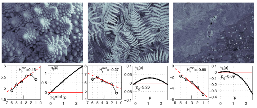
This estimation procedure has been studied in more detail in [16]. Three examples of its numerical application to real-world functions are provided in Figure 1.

A multifractal analysis based on the Hรถlder exponent can only be performed if $f$ is locally bounded. A way to determine if this is the case consists in first checking if ${H^{min}_{f}}>0$. This quantity is perfectly well-defined for mathematical functions or stochastic processes; e.g. for Brownian motion, ${H^{min}_{f}}=1/2$, and for Gaussian white noise, ${H^{min}_{f}}=-1/2$. However the situation may seem less clear for experimental signals; indeed any data acquisition device yields a finite set of locally averaged quantities, and one may argue that such a finite collection of data (which, by construction, is bounded) can indeed be modeled by a locally bounded function. This argument can only be turned by revisiting the way that (7) is computed in practice: Estimation is performed through a linear regression in log-log coordinates on the range of scales available in the data and ${H^{min}_{f}}$ can indeed be found negative for a finite collection of data. At the modeling level, this means that a mathematical model which would display the same linear behavior in log-log coordinates at all scales would satisfy ${H^{min}_{f}}<0$.

The quantity ${H^{min}_{f}}$ can be found either positive or negative depending on the nature of the application. For instance, velocity turbulence data and price time series in finance are found to always have ${H^{min}_{f}}>0$, while aggregated count Internet traffic time series always have ${H^{min}_{f}}<0$. For biomedical applications (cf. e.g., fetal heart rate variability) as well as for image processing, ${H^{min}_{f}}$ can commonly be found either positive or negative (see Figure 1) [2, 3, 16, 17, 28]. This raises the problem of using other pointwise regularity exponents that would not require the assumption that the data are locally bounded. We now introduce such exponents.

2.2. The $p$-exponent for $p\geq 1$

The introduction of $p$-exponents is motivated by the necessity of introducing regularity exponents that could be defined even when ${H^{min}_{f}}$ is found to be negative; $T^{p}_{\alpha}(x_{0})$ regularity, introduced by A. Calderรณn and A. Zygmund in [8], has the advantage of only making the assumption that $f$ locally belongs to $L^{p}({\mathbb{R}})$.

Definition 3.

Let $p\geq 1$ and assume that $f\in L^{p}_{loc}({\mathbb{R}})$. Let $\alpha\in{\mathbb{R}}$; the function $f$ belongs to $T^{p}_{\alpha}(x_{0})$ if there exists $C$ and a polynomial $P_{x_{0}}$ of degree less than $\alpha$ such that, for $r$ small enough,

(8) $$\left(\frac{1}{2r}\int_{x_{0}-r}^{x_{0}+r}|f(x)-P_{x_{0}}(x)|^{p}dx\right)^{1/p}\leq Cr^{\alpha}.$$

Note that the Taylor polynomial $P_{x_{0}}$ of $f$ at $x_{0}$ might depend on $p$. However, one can check that only its degree does (because the best possible ${\alpha}$ that one can pick in (8) depends on $p$ so that its integer part may vary with $p$, see [1]). Therefore we introduce no such dependency in the notation, which will lead to no ambiguity afterwards.

The $p$-exponent of $f$ at $x_{0}$ is defined as

(9) $$h_{f}^{p}(x_{0})=\sup\{\alpha:f\in T^{p}_{\alpha}(x_{0})\}.$$

The condition that $f$ locally belongs to $L^{p}({\mathbb{R}})$ implies that (8) holds for $\alpha=-1/p$, so that $h_{f}^{p}(x_{0})\geq-1/p$.

We will consider in the following โ€œarchetypicalโ€ pointwise singularities, which are simple toy-examples of singularities with a specific behavior at a point. They will illustrate the new notions we consider and they will also supply benchmarks on which we can compute exactly what these new notions allow us to quantify. These toy-examples will be a test for the adequacy between these mathematical notions and the intuitive behavior that we expect to quantify. The first (and most simple) โ€œarchetypicalโ€ pointwise singularities are the cusp singularities.

Let ${\alpha}\in{\mathbb{R}}-2{\mathbb{N}}$ be such that ${\alpha}>-1$. The cusp of order ${\alpha}$ at 00 is the function

(10) $${\mathcal{C}}_{{\alpha}}(x)=|x|^{\alpha}.$$

The case ${\alpha}\in 2{\mathbb{N}}$ is excluded because it leads to a $C^{\infty}$ function. However, if ${\alpha}=2n$, one can pick

$${\mathcal{C}}_{2n}(x)=x|x|^{2n-1},$$

in order to cover this case also.
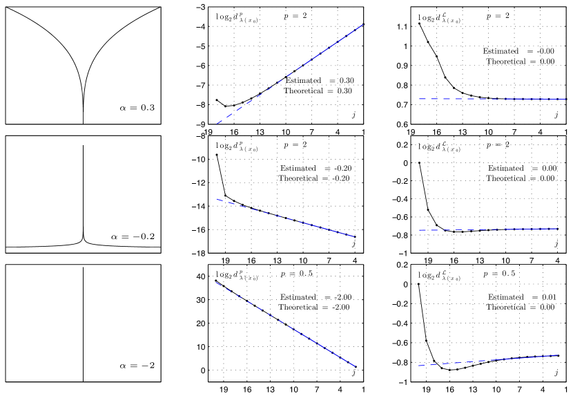
If ${\alpha}\geq 0$, then the cusp ${\mathcal{C}}_{{\alpha}}$ is locally bounded and its Hรถlder exponent at 00 is well-defined and takes the value ${\alpha}$. If ${\alpha}>-1/p$, then its $p$-exponent at 00 is well-defined and also takes the value ${\alpha}$, as in the Hรถlder case. (Condition ${\alpha}>-1/p$ is necessary and sufficient to ensure that ${\mathcal{C}}_{{\alpha}}$ locally belongs to $L^{p}$.) Examples for cusps with several different values of $\alpha$ are plotted in Figure 2.

If $f\in L^{p}_{loc}$ in a neighborhood of $x_{0}$ for a $p\geq 1$, let us define the critical Lebesgue index of $f$ at $x_{0}$ by

(11) $$p_{0}(f)=\sup\{p:f\in L^{p}_{loc}({\mathbb{R}})\mbox{ in a neighborhood of $x_{0}$}\}.$$

The importance of this exponent comes from the fact that it tells in practice for which values of $p$ a $p$-exponent based multifractal analysis can be performed. Therefore, its numerical determination is an important prerequisite that should not be bypassed in applications. In Section 3.1 we will extend the definition of $p_{0}(f)$ to situations where $f\notin L^{1}_{loc}$ and show how it can be derived from another quantity, the wavelet scaling function, which can be effectively computed on real-life data.

2.3. The lacunarity exponent

The $p$-exponent at $x_{0}$ is defined on the interval $[1,p_{0}(f)]$ or $[1,p_{0}(f))$; when the $p$-exponent does not depend on $p$ on this interval, we will say that $f$ has a $p$-invariant singularity at $x_{0}$. Thus, cusps are $p$-invariant singularities.

This first example raises the following question: Is the notion of $p$-exponent only relevant as an extension of the Hรถlder exponent to non-locally bounded functions? Or can it take different values with $p$, even for bounded functions? And, if such is the case, how can one characterize the additional information thus supplied? In order to answer this question, we introduce a second type of archetypical singularities, the lacunary singularities, which will show that the $p$-exponent may be non-constant. We first need to recall the geometrical notion of accessibility exponent which quantifies the lacunarity of a set at a point, see [19]. We denote by $\mathcal{M}(A)$ the Lebesgue measure of a set $A$.

Definition 4.

Let $\Omega\subset{\mathbb{R}}$. A point $x_{0}$ of the boundary of $\Omega$ is ${\alpha}$-accessible if there exist $C>0$ and $r_{0}>0$ such that $\forall r\leq r_{0}$,

(12) $$\mathcal{M}\left(\Omega\cap B(x_{0},r)\right)\leq Cr^{{\alpha}+1}.$$

The supremum of all values of ${\alpha}$ such that (12) holds is called the accessibility exponent of $\Omega$ at $x_{0}$. We will denote it by ${\mathcal{E}}_{x_{0}}(\Omega)$.

Note that ${\mathcal{E}}_{x_{0}}(\Omega)$ is always nonnegative. If it is strictly positive, then $\Omega$ is lacunary at $x_{0}$. The accessibility exponent supplies a way to estimate, through a log-log plot regression, the โ€œsizeโ€ of the part of $\Omega$ which is contained in arbitrarily small neighborhoods of $x_{0}$. The following sets illustrate this notion.

Let $\omega$ and $\gamma$ be such that $0<\gamma\leq\omega$; the set $U_{\omega,\gamma}$ is defined as follows. Let

(13) $$I^{j}_{\omega,\gamma}=[2^{-\omega j},2^{-\omega j}+2^{-\gamma j}];\quad\mbox{ then}\quad U_{\omega,\gamma}=\bigcup_{j\geq 0}I^{j}_{\omega,\gamma}.$$

Clearly, at the origin,

(14) $${\mathcal{E}}_{0}(U_{\omega,\gamma})=\frac{\gamma}{\omega}-1.$$

We now construct univariate functions $F_{{\alpha},\gamma}:{\mathbb{R}}\rightarrow{\mathbb{R}}$ which permit us to better understand the conditions under which $p$-exponents will differ. These functions will have a lacunary support in the sense of Definition 4.

Let $\psi$ be the Haar wavelet: $\psi=1_{[0,1/2)}-1_{[1/2,1)}$ and

$$\theta(x)=\psi(2x)-\psi(2x-1)$$

(so that $\theta$ has the same support as $\psi$ but its two first moments vanish).

Definition 5.

Let $\alpha\in{\mathbb{R}}$ and $\gamma>1$. The lacunary comb $F^{\alpha}_{\omega,\gamma}$ is the function

(15) $$F^{\alpha}_{\omega,\gamma}(x)=\sum_{j=1}^{\infty}2^{-{\alpha}j}\theta\left(2^{\gamma j}(x-2^{-\omega j})\right).$$

Note that its singularity is at $x_{0}=0$. Numerical examples of lacunary combs are provided in Figure 3.

Note that the support of $F^{\alpha}_{\omega,\gamma}$ is $U_{\omega,\gamma}$ so that the accessibility exponent at 0 of this support is given by (14). The function $F^{\alpha}_{\omega,\gamma}$ is locally bounded if and only if ${\alpha}\geq 0$. Assume that ${\alpha}<0$; then $F^{\alpha}_{\omega,\gamma}$ locally belongs to $L^{p}$ if and only if ${\alpha}>-\gamma/p$. When such is the case, a straightforward computation yields that its $p$-exponent at 0 is given by

(16) $$h_{F^{\alpha}_{\omega,\gamma}}^{p}(x_{0})=\frac{{\alpha}}{\omega}+\left(\frac{\gamma}{\omega}-1\right)\frac{1}{p}.$$

In contradistinction with the cusp case, the $p$-exponent of $F^{\alpha}_{\omega,\gamma}$ at 0 is not a constant function of $p$. Let us see how the variations of the mapping $p\rightarrow h^{p}_{f}(x_{0})$ are related with the lacunarity of the support of $f$, in the particular case of $F^{\alpha}_{\omega,\gamma}$. We note that this mapping is an affine function of the variable $q=1/p$ (which, in this context, is a more natural parameter than $p$) and that the accessibility exponent of the support of $F^{\alpha}_{\omega,\gamma}$ can be recovered by a derivative of this mapping with respect to $q$. The next question is to determine the value of $q$ at which this derivative should be taken. This toy-example is too simple to give a clue since any value of $q$ would lead to the same value for the derivative. We want to find if there is a more natural one, which would lead to a canonical definition for the lacunarity exponent. It is possible to settle this point through the following simple perturbation argument: Consider a new singularity $F$ that would be the sum of two functions $F_{1}=F^{{\alpha}_{1}}_{\omega_{1},\gamma_{1}}$ and $F_{2}=F^{{\alpha}_{2}}_{\omega_{2},\gamma_{2}}$ with

(17) $$0<{\alpha}_{1}<{\alpha}_{2}\quad\mbox{ and }\quad\gamma_{1}>\gamma_{2}.$$

The $p$-exponent of $F$ (now expressed in the $q$ variable, where $q=1/p$) is given by

(18) $$q\mapsto h_{f}^{\frac{1}{q}}(x_{0})=\min\left[\frac{{\alpha}_{1}}{\omega}+\left(\frac{\gamma_{1}}{\omega}-1\right)q\;,\;\;\frac{{\alpha}_{2}}{\omega}+\left(\frac{\gamma_{2}}{\omega}-1\right)q\right].$$

The formula for the lacunarity exponent should yield the lacunarity of the most irregular component of $F$; since $F\in L^{\infty}_{loc}$, the Hรถlder exponent is the natural way to measure this irregularity. In this respect, the most irregular component is $F_{1}$; the lacunarity exponent should thus take the value $\left(\frac{\gamma_{1}}{\omega}-1\right)$. But, since (17) allows the shift in slope of the function (18) from $\left(\frac{\gamma_{1}}{\omega}-1\right)$ to $\left(\frac{\gamma_{2}}{\omega}-1\right)$ to take place at a $q$ arbitrarily close to 00, the only way to obtain this desired result in any case is to pick the derivative of the mapping $q\rightarrow h^{1/q}_{f}(x_{0})$ precisely at $q=0$.

A similar perturbation argument can be developed if $p_{0}(f)<\infty$ with the conclusion that the derivative should be estimated at the smallest possible value of $q$, i.e. for

$$q=q_{0}(f):=\frac{1}{p_{0}(f)};$$

hence the following definition of the lacunarity exponent.

Definition 6.

Let $f\in L^{p}_{loc}$ in a neighborhood of $x_{0}$ for a $p>1$, and assume that the $p$-exponent of $f$ is finite in a left neighborhood of $p_{0}(f)$. The lacunarity exponent of $f$ at $x_{0}$ is

(19) $${\mathcal{L}}_{f}(x_{0})=\frac{\partial}{\partial q}\left(h_{f}^{1/q}(x_{0})\right)_{q=q_{0}(f)^{+}}.$$

Remarks:

  • โ€ข

    Even if the $p$-exponent is not defined at $p_{0}(f)$, nonetheless, because of the concavity of the mapping $q\rightarrow h^{1/q}_{f}(x_{0})$ (see Proposition 3.1 below), its right derivative is always well-defined, possibly as a limit.

  • โ€ข

    As expected, the lacunarity exponent of a cusp vanishes, whereas the lacunarity exponent of a lacunary comb coincides with the accessibility exponent of its support.

  • โ€ข

    The condition โ„’fโ€‹(x0)โ‰ 0subscriptโ„’๐‘“subscript๐‘ฅ00{\mathcal{L}}_{f}(x_{0})\neq 0 does not mean that the support of $f$ (or of $f-P$) has a positive accessibility exponent (think of the function $F^{\alpha}_{\omega,\gamma}+g$ where $g$ is a $C^{\infty}$ but nowhere polynomial function).

  • โ€ข

    The definition supplied by (19) bears similarity with the definition of the oscillation exponent (see [4, 16] and ref. therein) which is also defined through a derivative of a pointwise exponent; but the variable with respect to which the derivative is computed is the order of a fractional integration. The relationships between these two exponents will be investigated in a forthcoming paper [20].

3. Properties of the $p$-exponent

In signal and image processing, one often meets data that cannot be modeled by functions $f\in L^{1}_{loc}$, see Figure 1. It is therefore necessary to set the analysis in a wider functional setting, and therefore to extend the notion of $T^{p}_{\alpha}(x_{0})$ regularity to the case $p<1$.

3.1. The case $p<1$

The standard way to perform this extension is to consider exponents in the setting of the real Hardy spaces $H^{p}$ (with $p<1$) instead of $L^{p}$ spaces, see [14, 15]. First, we need to extend the definitions that we gave to the range $p\in(0,1]$. The simplest way is to start with the wavelet characterization of $L^{p}$ spaces, which we now recall.

We denote indifferently by $\chi_{j,k}$ or $\chi_{\lambda}$ the characteristic function of the interval ${\lambda}\;(={\lambda}_{j,k})$ defined by (6). The wavelet square function of $f$ is

$${\mathcal{W}}_{f}(x)=\left(\sum_{(j,k)\in{\mathbb{Z}}^{2}}|c_{j,k}|^{2}\chi_{j,k}(x)\right)^{1/2}.$$

Then, for $p>1$,

(20) $$f\in L^{p}({\mathbb{R}})\Longleftrightarrow\int_{\mathbb{R}}\left({\mathcal{W}}_{f}(x)\right)^{p}dx<\infty,$$

see [22]. The quantity $\left(\int\left({\mathcal{W}}_{f}(x)\right)^{p}dx\right)^{1/p}$ is thus equivalent to $\parallel f\parallel_{p}$. One can then take the characterization supplied by (20) when $p>1$ as a definition of the Hardy space $H^{p}$ (when $p\leq 1$); note that this definition yields equivalent quantities when the (smooth enough) wavelet basis is changed, see [22]. This justifies the fact that we will often denote by $L^{p}$ the space $H^{p}$, which will lead to no confusion; indeed, when $p\leq 1$ this notation will refer to $H^{p}$, and, when $p>1$ it will refer to $L^{p}$.

Note that, if $p=1$, (20) does not characterize the space $L^{1}$ but a strict subspace of $L^{1}$ (the real Hardy space $H^{1}$, which consists of functions of $L^{1}$ whose Hilbert transform also belongs to $L^{1}$, see [22]).

Most results proved for the $L^{p}$ setting will extend without modification to the $H^{p}$ setting. In particular, $T^{p}_{\alpha}$ regularity can be extended to the case $p\leq 1$ and has the same wavelet characterization, see [21]. All definitions introduced previously therefore extend to this setting.

The definition of $T^{p}_{\alpha}(x_{0})$ regularity given by (8) is a size estimate of an $L^{p}$ norm restricted to intervals $[x_{0}-r,x_{0}+r]$. Since the elements of $H^{p}$ can be distributions, the restriction of $f$ to an interval cannot be done directly (multiplying a distribution by a non-smooth function, such as a characteristic function, does not always make sense). This problem can be solved as follows: If $I$ is an open interval, one defines $\parallel f\parallel_{H^{p}(I)}=\inf\parallel g\parallel_{p}$, where the infimum is taken on the $g\in H^{p}$ such that $f=g$ on $I$. The $T^{p}_{\alpha}$ condition for $p\leq 1$ is then defined by:

$$f\in T^{p}_{\alpha}(x_{0})\quad\Longleftrightarrow\quad\parallel f\parallel_{H^{p}((x_{0}-r,x_{0}+r))}\leq C\;r^{{\alpha}+1/p},$$

also when $p<1$. We will show below that the $p$-exponent takes values in $[-1/p,+\infty]$.

3.2. When can one use $p$-exponents?

We already mentioned that, in order to use the Hรถlder exponent as a way to measure pointwise regularity, we need to check that the data are locally bounded, a condition which is implied by the criterion ${H^{min}_{f}}>0$, which is therefore used as a practical prerequisite. Similarly, in order to use a $p$-exponent based multifractal analysis, we need to check that the data locally belong to $L^{p}$ or $H^{p}$, a condition which can be verified in practice through the computation of the wavelet scaling function, which we now recall.

The Sobolev space Lp,ssuperscript๐ฟ๐‘๐‘ L^{p,s} is defined by

โˆ€sโˆˆโ„,โˆ€p>0,fโˆˆLp,sโŸบ(Iโ€‹dโˆ’ฮ”)s/2โ€‹fโˆˆLp,formulae-sequencefor-all๐‘ โ„formulae-sequencefor-all๐‘0formulae-sequence๐‘“superscript๐ฟ๐‘๐‘ โŸบsuperscript๐ผ๐‘‘ฮ”๐‘ 2๐‘“superscript๐ฟ๐‘\forall s\in{\mathbb{R}},\;\forall p>0,\qquad f\in L^{p,s}\quad\Longleftrightarrow\quad(Id-\Delta)^{s/2}f\in L^{p},

where the operator (Iโ€‹dโˆ’ฮ”)s/2superscript๐ผ๐‘‘ฮ”๐‘ 2(Id-\Delta)^{s/2} is the Fourier multiplier by (1+|ฮพ|2)s/2superscript1superscript๐œ‰2๐‘ 2(1+|\xi|^{2})^{s/2}, and we recall our convention that $L^{p}$ denotes the space $H^{p}$ when $p\leq 1$, so that Sobolev spaces are defined also for $p\leq 1$.

Definition 7.

Let $f$ be a tempered distribution. The wavelet scaling function of $f$ is defined by

(21) โˆ€p>0,ฮทfโ€‹(p)=pโ€‹sup{s:fโˆˆLp,s}.formulae-sequencefor-all๐‘0subscript๐œ‚๐‘“๐‘๐‘supremumconditional-set๐‘ ๐‘“superscript๐ฟ๐‘๐‘ \forall p>0,\qquad\eta_{f}(p)=p\;\sup\{s:f\in L^{p,s}\}.

Thus, $\forall p>0$:

  • โ€ข

    If $\eta_{f}(p)>0$ then $f\in L^{p}_{loc}$.

  • โ€ข

    If $\eta_{f}(p)<0$ then $f\notin L^{p}_{loc}$.

The wavelet characterization of Sobolev spaces implies that the wavelet scaling function can be expressed as (cf. [11])

(22) $$\forall p>0,\hskip 17.07164pt\eta_{f}(p)=\displaystyle\liminf_{j\rightarrow+\infty}\;\;\frac{\log\left(2^{-j}\displaystyle\sum_{k}|c_{j,k}|^{p}\right)}{\log(2^{-j})}.$$

This provides a practical criterion for determining if data locally belong to $L^{p}$, supplied by the condition $\eta_{f}(p)>0$. The following bounds for $p_{0}(f)$ follow:

$$\sup\{p:\eta_{f}(p)>0\}\leq p_{0}(f)\leq\inf\{p:\eta_{f}(p)<0\},$$

which (except in the very particular cases where $\eta_{f}$ vanishes identically on an interval) yields the exact value of $p_{0}(f)$.

In applications, data with very different values of $p_{0}(f)$ show up; therefore, in practice, the mathematical framework supplied by the whole range of $p$ is relevant. As an illustration, three examples of real-world images with positive and negative uniform Hรถlder exponents and with critical Lebesgue indices above and below $p_{0}=1$ are analyzed in Figure 1.

Refer to caption
Figure 1. Real-world images (top row) of Romanesco broccoli (left column), fern leaves (center column) and a patch of a hyperspectral image of the Moffett field, acquired by the AVIRIS instrument (spectral band 90, right column). Bottom row: corresponding numerical estimation of uniform Hรถlder exponents $H_{f}^{min}$, wavelet scaling functions $\eta_{f}(p)$ and critical Lebesgue indices $p_{0}$, respectively.

3.3. Wavelet characterization of $p$-exponents

In order to compute and prove properties of $p$-exponents we will need the exact wavelet characterization of $T^{p}_{\alpha}(x_{0})$, see [21, 14]. Let $\lambda$ be a dyadic interval; $3\lambda$ will denote the interval of same center and three times wider (it is the union of ${\lambda}$ and its two closest neighbors). For $x_{0}\in{\mathbb{R}}^{d}$, denote by $\lambda_{j}(x_{0})$ the dyadic cube of width $2^{-j}$ which contains $x_{0}$. The local square functions at $x_{0}$ are the sequences defined for $j\geq 0$ by

$${\mathcal{W}}^{j}_{f,x_{0}}(x)=\left(\sum_{{\lambda}\subset 3\lambda_{j}(x_{0})}|\ c_{\lambda}|^{2}\chi_{\lambda}(x)\right)^{1/2}.$$

Recall that (cf. [21])

(23) $$f\in T^{p}_{\alpha}(x_{0})\quad\mbox{ if and only if }\exists C>0,\;\forall j\geq 0\qquad\left\|{\mathcal{W}}^{j}_{f,x_{0}}\right\|_{p}\leq C\;2^{-({\alpha}+1/p)j}.$$

The following result is required for the definition of the lacunarity exponent in (19) to make sense, and implies that Definition 6 also makes sense when $p_{0}(f)<1$.

Proposition 3.1.

Let $p,q\in(0,+\infty]$, and suppose that $f\in T^{p}_{\alpha}(x_{0})\cap T^{q}_{\beta}(x_{0})$; let $\theta\in[0,1]$. Then $f\in T^{r}_{\gamma}(x_{0})$, where

$$\frac{1}{r}=\frac{\theta}{p}+\frac{1-\theta}{q}\quad\mbox{ and}\quad\gamma=\theta{\alpha}+(1-\theta)\beta.$$

It follows that the mapping $q\rightarrow h^{1/q}_{f}(x_{0})$ is concave on its domain of definition.

Proof: When $p,q<\infty$, the result is a consequence of (23). Hรถlderโ€™s inequality implies that

$$\left\|{\mathcal{W}}^{j}_{f,x_{0}}\right\|_{r}\leq\left\|{\mathcal{W}}^{j}_{f,x_{0}}\right\|^{\theta/p}_{p}\left\|{\mathcal{W}}^{j}_{f,x_{0}}\right\|^{(1-\theta)/q}_{q}.$$

We thus obtain the result for $p,q<\infty$. The case when $p$ or $q=+\infty$ does not follow, because there exists no exact wavelet characterization of $C^{\alpha}(x_{0})=T^{\infty}_{\alpha}(x_{0})$; however, when $p,q>1$, one can use the initial definition of $T^{p}_{\alpha}(x_{0})$ and $C^{\alpha}(x_{0})$ through local $L^{p}$ and $L^{\infty}$ norms and the result also follows from Hรถlderโ€™s inequality; hence Proposition 3.1 holds.

If $f\in H^{p}$, then $\parallel{\mathcal{W}}_{f}\parallel_{p}\leq C$. Since ${\mathcal{W}}^{j}_{f}\leq{\mathcal{W}}_{f}$, it follows that $\parallel{\mathcal{W}}^{j}_{f}\parallel_{p}\leq C$, so that (23) holds with ${\alpha}=-1/p$. Thus $p$-exponents are always larger than $-1/p$ (which extends to the range $p<1$ the result already mentioned for $p\geq 1$). Note that this bound is compatible with the existence of singularities of arbitrary large negative order (by picking $p$ close to 0). The example of cusps will now show that the $p$-exponent can indeed take values down to $-1/p$.

Refer to caption
Figure 2. Cusps with exponents $\alpha=\{+0.3,\;-0.2,\;-2\}$ (from top to bottom row, respectively): functions (left column) and estimation of $p$-exponents and lacunarity exponents (center and right column, respectively). The critical Lebesgue indices are given by $p_{0}=\{+\infty,\;5,\;0.5\}$, respectively.
Refer to caption
Figure 3. Lacunary combs with $p_{0}=+\infty$ (top row) and $p_{0}=9.1$ (bottom row): functions (left column) and estimation of $p$-exponents and lacunarity exponents (center and right column, respectively).

3.4. Computation of $p$-exponents for cusps

Typical examples of distributions for which the $p$-exponent is constant (see Proposition 3.2 below) and equal to a given value ${\alpha}<-1$ are supplied by the cusps ${\mathcal{C}}_{{\alpha}}$, whose definition can be extended to the range ${\alpha}\leq-1$ as follows: First, note that cusps cannot be defined directly for ${\alpha}\leq-1$ by (10) because they do not belong to $L^{1}_{loc}$ so that they would be ill-defined even in the setting of distributions (their integral against a $C^{\infty}$ compactly supported function $\varphi$ may diverge). Instead, we use the fact that, if ${\alpha}>1$, then ${\mathcal{C}}_{{\alpha}}^{\prime\prime}={\alpha}({\alpha}-1){\mathcal{C}}_{{\alpha}-2}$, which indicates a way to define by recursion the cusps ${\mathcal{C}}_{{\alpha}}$, when ${\alpha}<-1$ and ${\alpha}\notin{\mathbb{Z}}$, as follows:

 $$\mbox{ if }\quad{\alpha}<0,\qquad{\mathcal{C}}_{{\alpha}}=\frac{1}{({\alpha}+1)({\alpha}+2)}{\mathcal{C}}_{{\alpha}+2}^{\prime\prime},$$

where the derivative is taken in the sense of distributions. The ${\mathcal{C}}_{{\alpha}}$ are thus defined as distributions when ${\alpha}$ is not a negative integer. It can also be done when ${\alpha}$ is a negative integer, using the following definition for ${\alpha}=0$ and $-1$:

$${\mathcal{C}}_{0}=\log(|x|)\qquad\mbox{ and}\qquad{\mathcal{C}}_{-1}={\mathcal{C}}_{0}^{\prime}=P.V.\left(\frac{1}{x}\right),$$

where P.V. stands for โ€œprincipal valueโ€.

Proposition 3.2.

If ${\alpha}\geq 0$, the cusp ${\mathcal{C}}_{{\alpha}}$ belongs to $L^{\infty}_{loc}$ and its $p$-exponent is ${\alpha}$. If ${\alpha}<0$, the cusp ${\mathcal{C}}_{{\alpha}}$ belongs to $L^{p}_{loc}$ for $p<-1/{\alpha}$ and its $p$-exponent is ${\alpha}$.

Proof of Proposition 3.2: The case ${\alpha}\geq 0$ and $p\geq 1$ has already been considered in [20, 19]. In this case, the computation of the $p$-exponent is straightforward. Note that, when ${\alpha}\in(-1,0)$ and $p\geq 1$ the computations are similar. We thus focus on the distribution case, i.e. when $p<1$. The global and pointwise regularity will be determined through an estimation of the wavelet coefficients of the cusp. We use a smooth enough, compactly supported wavelet basis and we denote by $c_{j,k}$ the wavelet coefficients of the cusp

$$c_{j,k}=2^{j}\langle\psi_{j,k}|{\mathcal{C}}_{{\alpha}}\rangle.$$

The selfsimilarity of the cusp implies that

(24) $$\forall j,k\qquad c_{j,k}=2^{-{\alpha}j}c_{0,k};$$

additionally, as soon as $k$ is large enough so that the support of $\psi(x-k)$ does not intersect the origin, the cusp is $C^{\infty}$ in the support of $\psi(x-k)$ and coincides with the function $|x|^{\alpha}$. An integration by parts then yields that, for any $N$ smaller than the global regularity of the wavelet,

$$c_{0,k}=(-1)^{N}\int{\psi^{(-N)}}(x-k)\;{\alpha}({\alpha}-1)\cdots({\alpha}-N)|x|^{{\alpha}-N}dx,$$

so that the sequence $c_{0,k}$ satisfies

(25) $$|c_{0,k}|\leq\frac{C_{N}}{(1+|k|)^{N}}$$

where $N$ can be picked arbitrarily large. The estimation of the $L^{p}$ norm of the wavelet square function follows easily from (24) and (25), and so does the lower bound for the $p$-exponent. The upper bound is obtained by noticing that one of the $c_{0,k}$ does not vanish (otherwise, all $c_{j,k}$ would vanish, and the cusp would be a smooth function at the origin). Therefore, there exists at least one $k_{0}$ such that $\forall j$, $c_{j,k_{0}}=C2^{-{\alpha}j}$, and the wavelet characterization of $T^{p}_{\alpha}$ regularity then yields that $h^{p}(x_{0})\leq{\alpha}$.

Three examples of cusps and numerical estimates of their $p$-exponents and lacunarity exponents are plotted in Figure 2.

3.5. Wavelet characterization and thin chirps

In practice, we will derive $T^{p}_{\alpha}$ regularity from simpler quantities than the local square functions. The $p$-leaders of $f$ are defined by local $l^{p}$ norms of wavelet coefficients as follows:

(26) $$d_{\lambda}^{p}=\left(\sum_{\lambda^{\prime}\subset 3\lambda}|c_{\lambda^{\prime}}|^{p}2^{-(j^{\prime}-j)}\right)^{1/p}$$

(they are finite if $f\in L^{p}_{loc}({\mathbb{R}}^{d})$, see [19]). Note that, if $p=+\infty$, the corresponding quantity $d_{\lambda}^{\infty}$ is usually denoted by $d_{\lambda}$ and simply called the wavelet leaders; we have

(27) $$d_{\lambda}:=d_{\lambda}^{\infty}=\sup_{\lambda^{\prime}\subset 3\lambda}|c_{\lambda^{\prime}}|.$$

The notion of $T^{p}_{\alpha}$ regularity can be related to $p$-leader coefficients (see [15, 16, 19]):

(28)  $$\mbox{ If $\eta_{f}(p)>0$, then }\quad h^{p}_{f}(x_{0})=\liminf_{j\rightarrow+\infty}\;\;\frac{\log\left(d^{p}_{\lambda_{j}(x_{0})}\right)}{\log(2^{-j})}.$$
Refer to caption
Figure 4. Thin chirps with $p_{0}=\infty$ (top row) and $p_{0}=3.2$ (bottom row): functions (left column) and estimation of $p$-exponents and lacunarity exponents (center and right column, respectively).

Our purpose in this section is to introduce new โ€œarchetypicalโ€ pointwise singularities which will yield examples where the $p$-exponent and the lacunarity exponent can take arbitrary values. Because of (28), it is easier to work with examples that are defined directly by their wavelet coefficients on a smooth wavelet basis. We therefore develop new examples rather than extending the lacunary combs of Section 2.3.

Definition 8.

Let $a,b\in(0,1)$ satisfying $0<b<1-a$, and let ${\alpha}\in{\mathbb{R}}$. The thin chirp ${\mathcal{T}}_{a,b,{\alpha}}$ is defined by its wavelet series

$${\mathcal{T}}_{a,b,{\alpha}}=\sum_{j\geq 0}\;\sum_{k\in{\mathbb{Z}}}c_{j,k}\;\psi_{j,k},$$

where

$$\begin{array}[]{rll}c_{j,k}&=2^{-{\alpha}j}&\mbox{ if }\quad k\in[2^{(1-a)j},2^{(1-a)j}+2^{bj}]\\ &=0&\mbox{ otherwise. }\end{array}$$

The following results are straightforward, using the wavelet characterization of $L^{p}$ and $T^{p}_{\alpha}$ regularity.

Proposition 3.3.

The thin chirp ${\mathcal{T}}_{a,b,{\alpha}}$ is bounded if and only if ${\alpha}>0$.

 $$\mbox{ If}\quad{\alpha}\leq 0,\qquad p_{0}({\mathcal{T}}_{a,b,{\alpha}})=\frac{1-b}{-{\alpha}}.$$

The $p$-exponent of ${\mathcal{T}}_{a,b,{\alpha}}$ at the origin is

$$h^{p}_{{\mathcal{T}}_{a,b,{\alpha}}}(0)=\frac{1-a-b}{a}q+\frac{{\alpha}}{a}.$$

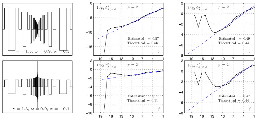
Note that, if the wavelets are compactly supported, then for $j$ large enough the pack of $2^{bj}$ successive wavelets with non-vanishing coefficients covers an interval of length $2^{-j}2^{bj}$ at a distance $2^{-aj}$ from the origin, so that the accessibility exponent of the support of ${\mathcal{T}}_{a,b,{\alpha}}$ is $(1-a-b)/a$: Thus, it coincides with the lacunarity exponent of ${\mathcal{T}}_{a,b,{\alpha}}$ as expected.

Illustrations of thin chirps and the numerical estimation of their $p$-exponents and lacunarity exponents are provided in Figure 4.

3.6. $p$-exponent analysis of measures

Several types of measures (such as multiplicative cascades) played a central role in the development of multifractal analysis. Since measures (usually) are not $L^{1}$ functions, their $p$-exponent for $p\geq 1$ is not defined. Therefore, it is natural to wonder if it can be the case when $p<1$. This is one of the purposes of Proposition 3.4, which yields sufficient conditions under which a measure $\mu$ satisfies $\eta_{\mu}(p)>0$ for $p<1$, which will imply that its $p$-exponent multifractal analysis can be performed. An important by-product of using $p$-exponents for $p\leq 1$ is that it offers a common setting to treat pointwise regularity of measures and functions.

Recall that $\overline{\dim_{B}}(A)$ denotes the upper box dimension of the set $A$.

Proposition 3.4.

Let $\mu$ be a measure; then its wavelet scaling function satisfies $\eta_{\mu}(1)\geq 0$. Furthermore, if $\mu$ does not have a density which is an $L^{1}$ function, then $\eta_{\mu}(1)=0.$

Additionally, if $\mu$ is a singular measure whose support sโ€‹uโ€‹pโ€‹pโ€‹(ฮผ)๐‘ ๐‘ข๐‘๐‘๐œ‡supp(\mu) satisfies

(29) ฮดฮผ:=dimBยฏโ€‹(sโ€‹uโ€‹pโ€‹pโ€‹(ฮผ))<1,assignsubscript๐›ฟ๐œ‡ยฏsubscriptdimension๐ต๐‘ ๐‘ข๐‘๐‘๐œ‡1\delta_{\mu}:=\overline{\dim_{B}}(supp(\mu))<1,

then

(30) $$\forall p<1,\qquad\eta_{\mu}(p)\geq{(1-\delta_{\mu})}{(1-p)},$$

and

(31) $$\forall p>1,\qquad\eta_{\mu}(p)\leq{(1-\delta_{\mu})}{(1-p)}.$$

Remarks:

  • โ€ข

    (30) expresses the fact that, if $\mu$ has a small support, then its Sobolev regularity is increased for $p<1$. This is somehow counterintuitive, since one expects a measure to become more singular when the size of its support shrinks; on the other hand (31) expresses that this is actually the case when $p>1$.

  • โ€ข

    Condition $\delta_{\mu}<1$ is satisfied if $\mu$ is supported by a Cantor-like set, or by a selfsimilar set satisfying Hutchinsonโ€™s open set condition.

  • โ€ข

    (30) has an important consequence for the multifractal analysis of measures: Indeed, if $\delta_{\mu}<1$, then $\eta_{\mu}(p)>0$ for $p<1$, so that the classical mathematical results concerning the multifractal analysis based on the $p$-exponent apply, see Section 4.

  • โ€ข

    A slightly different problem was addressed by H. Triebel: In [27], he determined under which conditions the scaling functions commonly used in the multifractal analysis of probability measures (see (37) below) can be recovered through Besov or Triebel-Lizorkin norms (or semi-norms).

Proof of Proposition 3.4: If $\mu$ is a measure, then for any continuous bounded function $f$

(32) $$|\langle\mu|f\rangle|\leq C\parallel f\parallel_{\infty}.$$

We pick

$$f=\sum_{k}{\varepsilon}_{j,k}\psi_{j,k},\qquad\mbox{ where}\quad{\varepsilon}_{j,k}=\pm 1,$$

so that $f$ is continuous and satisfies $\parallel f\parallel_{\infty}\leq C$, where $C$ depends only on the wavelet (but not on the choice of the ${\varepsilon}_{j,k}$). Denoting by $c_{j,k}$ the wavelet coefficients of $\mu$, we have

$$\langle\mu|f\rangle=\sum_{k}{\varepsilon}_{j,k}\int\psi_{j,k}d\mu=2^{-j}\sum_{k}{\varepsilon}_{j,k}c_{j,k}.$$

Picking ${\varepsilon}_{j,k}=\mbox{sgn}(c_{j,k})$ it follows from (32) that

(33) $$2^{-j}\sum_{k}|c_{j,k}|\leq C,$$

or, in other words, $\mu$ belongs to the Besov space $B^{0,\infty}_{1}$, which implies that $\eta_{\mu}(1)\geq 0$, see [13, 22].

On other hand, if $\mu\notin L^{1}$, then using the interpretation of the scaling function in terms of Sobolev spaces given by (21), we obtain that $\eta_{\mu}(1)\leq 0$. Hence the first part of the proposition holds.

We now prove (30). We assume that the used wavelet is compactly supported, and that its support is included in the interval $[-2^{l},2^{l}]$ for an $l>0$ (we pick the smallest $l$ such that this is possible). Let ฮด>dimBยฏโ€‹(sโ€‹uโ€‹pโ€‹pโ€‹(ฮผ))๐›ฟยฏsubscriptdimension๐ต๐‘ ๐‘ข๐‘๐‘๐œ‡\delta>\overline{\dim_{B}}(supp(\mu)); for $j$ large enough, sโ€‹uโ€‹pโ€‹pโ€‹(ฮผ)๐‘ ๐‘ข๐‘๐‘๐œ‡supp(\mu) is included in at most $2^{[\delta j]}$ intervals of length $2^{-j}$. It follows that, at scale $j$, there exist at most $2^{[\delta j]}\cdot 2\cdot 2^{l}$ wavelets $(\psi_{j,k})_{k\in{\mathbb{Z}}}$ whose support intersects the support of $\mu$. Thus for $j$ large enough, there are at most $C2^{\delta j}$ wavelet coefficients that do not vanish.

Let $p\in(0,1)$, $q=1/p$ and $r$ be the conjugate exponent of $q$, i.e. such that $1/q+1/r=1$. Using Hรถlderโ€™s inequality,

$$\sum_{k}|c_{j,k}|^{p}\leq\left(\sum_{k}|c_{j,k}|^{pq}\right)^{1/q}\left(\sum_{k}1^{r}\right)^{1/r},$$

where the sums are over at most $C2^{\delta j}$ terms; thus

$$\sum_{k}|c_{j,k}|^{p}\leq\left(\sum_{k}|c_{j,k}|\right)^{p}\;C\,2^{\delta j/r}.$$

Using (33), we obtain that

$$2^{-j}\sum_{k}|c_{j,k}|^{p}\leq C2^{-(1-\delta)j/r},$$

so that $\eta_{\mu}(p)\geq(1-\delta)(1-p)$. Since this is true $\forall\delta>\delta_{\mu}$, (30) follows.

We now prove (31). Let $p\geq 1$ and let $q$ be the conjugate exponent. Using Hรถlderโ€™s inequality,

$$\sum_{k}|c_{j,k}|\leq\left(\sum_{k}|c_{j,k}|^{p}\right)^{1/p}\left(\sum_{k}1^{q}\right)^{1/q}.$$

Let again $\delta>\delta_{\mu}$; using the fact that the sums bear on at most $2^{\delta j}$ terms, and that the left-hand side is larger than $C2^{j}$, we obtain that

$$\left(\sum_{k}|c_{j,k}|^{p}\right)^{1/p}\geq C\;2^{j}2^{-\delta j/q},$$

which can be rewritten

$$2^{-j}\sum_{k}|c_{j,k}|^{p}\geq C\;2^{-j}2^{pj}2^{-\delta jp/q},$$

so that $\eta_{\mu}(p)\leq(1-p)(1-\delta)$; since this is true $\forall\delta>\delta_{\mu}$, (31) follows, and Proposition 3.4 is completely proved.

Since $p=1$ is a borderline case for the use of the $1$-exponent one may expect that picking $p<1$ would yield $\eta_{\mu}(p)>0$ (in which case one would be on the safe side in order to recover mathematical results concerning the $p$-spectrum, see [14, 1]). However, this is not the case, since there exist even continuous functions $f$ that satisfy $\forall p>0$, $\eta_{f}(p)=0$. An example is supplied by

$$f=\sum_{j\geq 0}\sum_{k\in{\mathbb{Z}}}\;\frac{1}{j^{2}}\,\psi_{j,k}.$$

4. Multifractal analysis of lacunary wavelet series

Multifractal analysis is motivated by the observation that many mathematical models have an extremely erratic pointwise regularity exponent which jumps everywhere; this is the case e.g. of multiplicative cascades or of Lรฉvy processes, whose exponents $h$ satisfy that

(34)  $$\mbox{ a.s.}\quad\forall x_{0},\qquad\limsup_{x_{\rightarrow}x_{0}}h(x)-\liminf_{x_{\rightarrow}x_{0}}h(x)$$

is bounded from below by a fixed positive quantity (we will see that this is also the case for lacunary wavelet series). This clearly excludes the possibility of any robust direct estimations of $h$. The driving idea of multifractal analysis is that one should rather focus on alternative quantities that

  • โ€ข

    are numerically computable on real life data in a stable way,

  • โ€ข

    yield information on the erratic behavior of the pointwise exponent.

Furthermore, for standard random models (such as the ones mentioned above) we require these quantities not to be random (i.e. not to depend on the sample path which is observed) but to depend on the characteristic parameters of the model only. The relationship between the multifractal spectrum and scaling functions (initially pointed out by U. Frisch and G. Parisi in [23]; see (39) below) satisfies these requirements.

We now recall the notion of multifractal spectrum. We denote by $\dim(A)$ the Hausdorff dimension of the set $A$.

Definition 9.

Let $h(x)$ denote a pointwise exponent. The multifractal spectrum $d(H)$ associated with this pointwise exponent is

$$d(H)=\dim\{x:\;\;h(x)=H\}.$$

In the case of the $p$-exponent, the sets of points with a given $p$-exponent will be denoted by $F^{p}_{f}(H)$:

(35) $$F^{p}_{f}(H)=\{x_{0}:\;h^{p}_{f}(x_{0})=H\},$$

and the corresponding multifractal spectrum (referred to as the $p$-spectrum) is denoted by $d^{p}(H)$; in the case of the lacunarity exponent, we denote it by $d^{\mathcal{L}}(L)$.

4.1. Derivation of the multifractal formalism

We now recall how $d(H)$ is expected to be recovered from global quantities effectively computable on real-life signals (following the seminal work of G. Parisi and U. Frisch [23] and its wavelet leader reinterpetation [13]). A key assumption is that this exponent can be derived from nonnegative quantities (which we denote either by $e_{j,k}$ or $e_{\lambda}$), which are defined on the set of dyadic intervals, by a log-log plot regression:

(36) $$h(x_{0})=\liminf_{j\rightarrow+\infty}\;\;\frac{\log\left(e_{\lambda_{j}(x_{0})}\right)}{\log(2^{-j})}.$$

It is for instance the case of the $p$-exponent, as stated in (23) or (28), for which the quantities $e_{\lambda}$ are given by the $p$-leaders $d^{p}_{\lambda}$.

In the case of the lacunarity exponent, quantities $e_{\lambda}$ can be derived as follows: Let $\Delta q>0$ small enough be given. If $f$ has a $1/q$-exponent $H$ and a lacunarity exponent $L$ at $x_{0}$ then its $1/q$-leaders satisfy

$$d^{1/q}_{j}(x_{0})\sim 2^{-Hj},$$

and its $1/(q+\Delta q)$-leaders satisfy

$$d^{1/(q+\Delta q)}_{j}(x_{0})\sim 2^{-(H+\Delta qL)j};$$

we can eliminate $H$ from these two quantities by considering the ${\mathcal{L}}$-leaders:

$$d^{\mathcal{L}}_{\lambda}:=\left(\frac{d^{1/(q+\Delta q)}_{j}}{d^{1/q}_{j}}\right)^{1/\Delta q}\sim 2^{-Lj}.$$

(this argument follows a similar one developed in [16, Ch. 4.3] for the derivation of a multifractal analysis associated with the oscillation exponent).

The multifractal spectrum will be derived from the following quantities, referred to as the structure functions, which are similar to the ones that come up in the characterization of the wavelet scaling function in (22):

$$S_{f}(r,j)=\left(2^{-j}\displaystyle\sum_{k}|e_{j,k}|^{r}\right).$$

The scaling function associated with the collection of $(e_{\lambda})$ is

(37) $$\forall r\in{\mathbb{R}},\hskip 17.07164pt\zeta_{f}(r)=\displaystyle\liminf_{j\rightarrow+\infty}\;\;\frac{\log\left(S_{f}(r,j)\right)}{\log(2^{-j})}.$$

Let us now sketch the heuristic derivation of the multifractal formalism; (37) means that, for large $j$,

$$S_{f}(r,j)\sim 2^{-{\zeta}(r)j}.$$

Let us estimate the contribution to $S_{f}(r,j)$ of the dyadic intervals ${\lambda}$ that cover the points of $E_{H}$. By definition of $E_{H}$, they satisfy $e_{\lambda}\sim 2^{-Hj};$ by definition of $d(H)$, since we use cubes of the same width $2^{-j}$ to cover $E_{H}$, we need about $2^{d(H)j}$ such cubes; therefore the corresponding contribution is of the order of magnitude of

$$2^{-j}2^{d(H)j}2^{-Hrj}=2^{-(1-d(H)+Hr)j}.$$

When $j\rightarrow+\infty$, the dominant contribution comes from the smallest exponent, so that

(38) $${\zeta}(r)=\inf_{H}(1-d(H)+Hr).$$

By construction, the scaling function ${\zeta}(r)$ is a concave function on ${\mathbb{R}}$, see [23, 13, 24] which is in agreement with the fact that the right-hand side of (38) necessarily is a concave function (as an infimum of a family of linear functions) no matter whether $d(H)$ is concave or not. If $d(H)$ also is a concave function, then the Legendre transform in (38) can be inverted (as a consequence of the duality of convex functions), which justifies the following assertion.

Definition 10.

A nonnegative sequence $(e_{\lambda})$, defined on the dyadic intervals, follows the multifractal formalism if the associated multifractal spectrum $d(H)$ satisfies

(39) $$d(H)=\inf_{r\in{\mathbb{R}}}(1-{\zeta}(r)+Hr).$$

The derivation given above is not a mathematical proof, and the determination of the range of validity of (39) (and of its variants) is one of the main mathematical problems concerning multifractal analysis. If it does not hold in complete generality, the multifractal formalism nevertheless yields an upper bound of the spectrum of singularities, see [23, 13, 24]: As soon as (36) holds,

$$d(H)\leq\inf_{r\in{\mathbb{R}}}(1-{\zeta}(r)+Hr).$$

In applications, multifractal analysis is often used only as a classification tool in order to discriminate between several types of signals; then, one is not directly concerned with the validity of (39) but only with a precise computation of the new multifractal parameters supplied by the scaling function, or equivalently its Legendre transform. Note that studies of multifractality for the $p$-exponent have been performed by A. Fraysse who proved genericity results of multifractality for functions in Besov or Sobolev spaces in [10].

4.2. Description of the model and global regularity

In this section, we extend to possibly negative exponents the model of lacunary wavelet series introduced in [12]. We assume that $\psi$ is a wavelet in the Schwartz class (see however the remark after Theorem 1, which gives sufficient conditions of validity of the results of this section when wavelets of limited regularity are used). Lacunary wavelet series depend on a lacunarity parameter $\eta\in(0,1)$ and a regularity parameter ${\alpha}\in{\mathbb{R}}$. At each scale $j\geq 0$, the process $X_{{\alpha},\eta}$ has exactly $[2^{\eta j}]$ nonvanishing wavelet coefficients on each interval $[l,l+1)$ ($l\in{\mathbb{Z}}$), their common size is $2^{-{\alpha}j}$, and their locations are picked at random: In each interval $[l,l+1)$ ($l\in{\mathbb{Z}}$), all drawings of $[2^{\eta j}]$ among the $2^{j}$ possibilities $\frac{k}{2^{j}}\in[l,l+1)$ have the same probability. Such a series is called a lacunary wavelet series of parameters $({\alpha},\eta)$. Note that, since ${\alpha}$ can be arbitrarily negative, $X_{{\alpha},\eta}$ can actually be a random distribution of arbitrary large order. By construction

$$H^{min}_{X_{{\alpha},\eta}}={\alpha},$$

and, more precisely, the sample paths of $X_{{\alpha},\eta}$ are locally bounded if and only if ${\alpha}>0$. The case considered in [12] dealt with ${\alpha}>0$, and was restricted to the computation of Hรถlder exponents. Considering $p$-exponents allows us to extend the model to negative values of ${\alpha}$, and also to see how the global sparsity of the wavelet expansion (most wavelet coefficients vanish) is related with the pointwise lacunarity of the sample paths. Note that extensions of this model in different directions have been worked out in [5, 9]

Since we are interested in local properties of the process $X$, we restrict our analysis to the interval $[0,1)$ (the results proved in the following clearly do not depend on the particular interval which is picked); we can therefore assume that $k\in\{0,\cdots 2^{j}-1\}$.

We first determine how ${\alpha}$ and $\eta$ are related with the global regularity of the sample paths. The characterization (22) implies that the wavelet scaling function is given by

(40) $$\forall p>0,\qquad\eta_{X_{{\alpha},\eta}}(p)={\alpha}p-\eta+1.$$

It follows that

$$p_{0}:=p_{0}(X_{{\alpha},\eta})=\begin{cases}\frac{\eta-1}{{\alpha}}&\mbox{if }\alpha<0\\ +\infty&\mbox{if }\alpha>0.\end{cases}$$

Note that $p_{0}$ always exists and is strictly positive, even if ${\alpha}$ takes arbitrarily large negative values. We recover the fact that $p$-exponents allow us to deal with singularities of arbitrarily large negative order. We will see that this is a particular occurrence of a general result, see Proposition 5.1; the key property here is the sparsity of the wavelet series.

4.3. Estimation of the $p$-leaders of $X_{{\alpha},\eta}$

An important step in the determination of the $p$-exponent of sample paths of $X_{{\alpha},\eta}$ at every point is the estimation of their $p$-leaders. We now assume that $p<p_{0}$, so that the sample paths of $X_{{\alpha},\eta}$ locally belong to $L^{p}$ and the $p$-exponent of $X_{{\alpha},\eta}$ is well-defined everywhere. Recall that the $p$-leaders are defined by

(41) $$l_{\lambda}=\left(\sum_{{\lambda}^{\prime}\subset 3{\lambda}}|c_{{\lambda}^{\prime}}|^{p}2^{-(j^{\prime}-j)}\right)^{1/p}.$$

The derivation of the $p$-exponent of $X_{{\alpha},\eta}$ everywhere will be deduced from the estimation of the size of the $p$-leaders of $X_{{\alpha},\eta}$. A key result is supplied by the following proposition, which states that the size of the $p$-leaders of a lacunary wavelet series is correctly estimated by the size of the first nonvanishing wavelet coefficient of smaller scale that is met in the set $\{{\lambda}^{\prime}:\;\;{\lambda}^{\prime}\subset 3{\lambda}\}$.

Proposition 4.1.

Let ${\alpha}\in{\mathbb{R}}$, $\eta\in(0,1)$ and let $X_{{\alpha},\eta}$ be a lacunary wavelet series of parameters $({\alpha},\eta)$; for each dyadic interval ${\lambda}$ (of width $2^{-j}$), we define $j^{\prime}$ ( $=j^{\prime}({\lambda})$) as the smallest random integer such that

โˆƒฮปโ€ฒโŠ‚3โ€‹ฮปโ€‹ such that โ€‹|ฮปโ€ฒ|=2โˆ’jโ€ฒโ€‹ andcฮปโ€ฒโ‰ 0.formulae-sequencesuperscript๐œ†โ€ฒ3๐œ† such that superscript๐œ†โ€ฒsuperscript2superscript๐‘—โ€ฒ andsubscript๐‘superscript๐œ†โ€ฒ0\exists{\lambda}^{\prime}\subset 3{\lambda}\;\;\mbox{ such that }|{\lambda}^{\prime}|=2^{-j^{\prime}}\;\;\mbox{ and}\quad c_{{\lambda}^{\prime}}\neq 0.

Then, a.s. $\exists J$, $\exists C,C^{\prime}>0$ such that $\forall j\geq J$, $\forall{\lambda}$ of scale $j$

$$\qquad C2^{-{\alpha}j^{\prime}}2^{-(j^{\prime}-j)/p}\leq l_{\lambda}\leq C^{\prime}2^{-{\alpha}j^{\prime}}2^{-(j^{\prime}-j)/p}j^{2/p}$$

Proof: This result will be implied by the exponential decay rate $2^{-(j^{\prime}-j)}$ that appears in the definition of $p$-leaders together with the lacunarity of the construction; we will show that exceptional situations where this would not be true (as a consequence of local accumulations of nonvanishing coefficients) have a small probability and ultimately will be excluded by a Borel-Cantelli type argument. We now make this argument precise. For that purpose, we will need to show that the sparsity of wavelet coefficients is uniform, which will be expressed by a uniform estimate on the maximal number of nonvanishing coefficients $c_{{\lambda}^{\prime}}$ that can be found for ${\lambda}^{\prime}$ (at a given scale $j^{\prime}$) included in a given interval $3{\lambda}$. Such an estimate can be derived by interpreting the choice of the nonvanishing wavelet coefficients in the construction of the model as a coarsening (on the dyadic grid) of an empirical process. Let us now recall this notion, and the standard estimate on the increments of the empirical process that we will need.

Let $N_{j}=[2^{\eta j}]$ denote the number of nonvanishing wavelet coefficients at scale $j$. We can consider that the corresponding dyadic intervals ${\lambda}$ have been obtained first by picking at random $N_{j}$ points in the interval $[0,1]$ (these points are now $N_{j}$ independent uniformly distributed random variables on $[0,1]$), and then by associating to each point the unique dyadic interval of scale $j$ to which it belongs. Let $P^{j}_{t}$ be the process starting from 0 at $t=0$, which is piecewise constant and which jumps by 1 at each random point thus determined. The family of processes

(42) $$\alpha^{j}_{t}=\sqrt{N_{j}}\left(\frac{P^{j}_{t}}{N_{j}}-t\right)$$

is called an empirical process on $[0,1]$. The size of the increments of the empirical process on a given interval yields information on the number of random points picked in this interval. If it is of length $l$, then the expected number of points is $l[2^{\eta j}]$, and the deviation from this average can be uniformly bounded using the following result of W. Stute which is a particular case of Lemma 2.4 of [26].

Lemma 4.2.

There exist two positive constants $C^{\prime}_{1}$ and $C^{\prime}_{2}$ such that, if $0<l<1/8$, $N_{j}l\geq 1$ and $8\leq A\leq C^{\prime}_{1}\sqrt{N_{j}l}$,

IPโ€‹(sup|tโˆ’s|โ‰คl|ฮฑtjโˆ’ฮฑsj|>Aโ€‹l)โ‰คC2โ€ฒlโ€‹eโˆ’A2/64.IPsubscriptsupremum๐‘ก๐‘ ๐‘™subscriptsuperscript๐›ผ๐‘—๐‘กsubscriptsuperscript๐›ผ๐‘—๐‘ ๐ด๐‘™subscriptsuperscript๐ถโ€ฒ2๐‘™superscript๐‘’superscript๐ด264{\rm I\kern-2.0ptP}\left(\sup_{|t-s|\leq l}|\alpha^{j}_{t}-\alpha^{j}_{s}|>A\sqrt{l}\right)\leq\frac{C^{\prime}_{2}}{l}e^{-A^{2}/64}.

Rewritten in terms of $P^{j}_{t}$, this means that

(43) IPโ€‹(sup|tโˆ’s|โ‰คl|Ptjโˆ’Psjโˆ’Njโ€‹(tโˆ’s)|>Aโ€‹Njโ€‹l)โ‰คC2โ€ฒlโ€‹eโˆ’A2/64.IPsubscriptsupremum๐‘ก๐‘ ๐‘™subscriptsuperscript๐‘ƒ๐‘—๐‘กsubscriptsuperscript๐‘ƒ๐‘—๐‘ subscript๐‘๐‘—๐‘ก๐‘ ๐ดsubscript๐‘๐‘—๐‘™subscriptsuperscript๐ถโ€ฒ2๐‘™superscript๐‘’superscript๐ด264{\rm I\kern-2.0ptP}\left(\sup_{|t-s|\leq l}|P^{j}_{t}-P^{j}_{s}-N_{j}(t-s)|>A\sqrt{N_{j}l}\right)\leq\frac{C^{\prime}_{2}}{l}e^{-A^{2}/64}.

Recall that the assumption $\lambda^{\prime}\subset 3\lambda$ implies that $3\cdot 2^{-j}\geq 2^{-j^{\prime}}$. We will apply Lemma 4.2 differently for small values of $j^{\prime}$ where the expected number of nonvanishing coefficients $c_{{\lambda}^{\prime}}$ that can be found for ${\lambda}^{\prime}$ (at a given scale $j^{\prime}$) included in a given interval ${\lambda}$ is very small, and the case of large $j^{\prime}$ where this number increases geometrically.

We first assume that

(44) $$2^{-j^{\prime}}\geq j^{2}2^{-j/\eta}.$$

We pick intervals of length $l={j^{\prime}}^{2}2^{-\eta j^{\prime}}$ and, for the constant $A$ in Stuteโ€™s lemma, we pick $A=j$. Then (43) applied with $N=[2^{\eta j^{\prime}}]$ yields that, with probability at least $1-e^{-j^{2}}$, the number of intervals ${\lambda}^{\prime}$ of scale $j^{\prime}$ picked in such intervals is

$$2^{\eta j^{\prime}}l+O(j^{2})=O(j^{2}).$$

We now assume that

(45) $$2^{-j^{\prime}}\leq j^{2}2^{-j/\eta}.$$

Then we pick intervals of length $l=3\cdot 2^{-j}$, and $A=j+j^{\prime}$. Then (43) applied with $N=[2^{\eta j^{\prime}}]$ yields that, with probability at least $1-e^{-(j+j^{\prime})^{2}}$, the number of intervals ${\lambda}^{\prime}$ of scale $j^{\prime}$ picked in such intervals is

(46) $$2^{\eta j^{\prime}}l+O((j+j^{\prime})^{2}\sqrt{2^{\eta j^{\prime}}l})\leq 2\cdot 2^{\eta j^{\prime}}l.$$

We are now ready to estimate the size of $l_{\lambda}$, assuming that all events described above happen (indeed, we note that the probabilities such that these events do not happen have a finite sum, so that, by the Borel-Cantelli lemma, they a.s. all occur for $j$ large enough).

At scales $j^{\prime}$ which satisfy (44), if at least one of the ${\lambda}^{\prime}\subset 3{\lambda}$ does not vanish, then there are at most $j^{2}$ of them, and the corresponding contribution to the sum in (41) lies between $|(c_{{\lambda}^{\prime}})^{p}2^{-(j-j^{\prime})}|$ and $j^{2}|(c_{{\lambda}^{\prime}})^{p}2^{-(j-j^{\prime})}|$. At scales $j^{\prime}$ which satisfy (45), the contribution of the wavelet coefficients of scale $j^{\prime}$ to the sum lies between $2^{\eta j^{\prime}l}|(c_{{\lambda}^{\prime}})^{p}2^{-(j-j^{\prime})}|$ and its double. Since $c_{{\lambda}^{\prime}}=2^{-{\alpha}j^{\prime}}$, the condition $p<p_{0}$ implies that these quantities decay geometrically, so that the order of magnitude of the $p$-leader is given by the first non-vanishing term in the sum. Hence Proposition 4.1 holds.

4.4. $p$-exponents and lacunarity

We now derive the consequences of Proposition 4.1 for the determination of the $p$-exponents of $X_{{\alpha},\eta}$ at every point. We first determine the range of $p$-exponents. First, note that all $p$-leaders have size at most $2^{-{\alpha}j}$, so that the $p$-exponent is everywhere larger than ${\alpha}$. In the opposite direction, as a consequence of (46), every interval $3{\lambda}$ of scale $j$ includes at least one nonvanishing wavelet coefficient at scale $j/\eta+(\log j)^{2}$; therefore, all $p$-leaders have size at least

$$2^{-{\alpha}\left(\frac{j}{\eta}+\log j\right)^{2}-\frac{1}{p}\left(\frac{j}{\eta}-j+(\log j)^{2}\right)}.$$

It follows that the $p$-exponents are everywhere smaller than

(47) $$H_{max}:=\frac{{\alpha}}{\eta}+\left(\frac{1}{\eta}-1\right)\frac{1}{p}.$$

We have thus obtained that

 $$\mbox{ a.s.}\qquad\forall p<p_{0},\;\forall x_{0}\in{\mathbb{R}},\qquad{\alpha}\leq h^{p}_{X_{{\alpha},\eta}}(x_{0})\leq H_{max}.$$

For each $j$, let $E^{j}_{\omega}$ denote the subset of $[0,1]$ composed of intervals $3{\lambda}$ (${\lambda}\in{\Lambda}_{j}$) inside which the first nonvanishing wavelet coefficient is attained at a scale $l\leq[\omega j]$, and let

$$E_{\omega}=\limsup E^{j}_{\omega}.$$

Proposition 4.1 implies that, if $x_{0}\notin E_{\omega}$, then, for $j$ large enough, all wavelet leaders $l_{{\lambda}_{j}(x_{0})}$ are bounded by

$$j^{2}2^{-{\alpha}\frac{j}{\eta}-\frac{1}{p}\left(\frac{j}{\eta}-j\right)},$$

so that:

(48)  $$\mbox{ if $x_{0}\notin E_{\omega}$, then }\qquad h^{p}_{X_{{\alpha},\eta}}(x_{0})\geq{{\alpha}}{\omega}+\frac{\omega-1}{p}.$$

On other hand, if $x_{0}\in E_{\omega}$, then there exists an infinite number of $p$-leaders $l_{{\lambda}_{j}(x_{0})}$ larger than

$$2^{-{\alpha}\frac{j}{\eta}-\frac{1}{p}\left(\frac{j}{\eta}-j\right)},$$

so that:

(49)  $$\mbox{ if $x_{0}\in E_{\omega}$, then }\qquad h^{p}_{X_{{\alpha},\eta}}(x_{0})\leq{{\alpha}}{\omega}+\frac{\omega-1}{p}.$$

It follows from (48) and (49) that the sets of points where the $p$-exponent takes the value

$$H={{\alpha}}{\omega}+\frac{\omega-1}{p}$$

are the sets

$$H_{\omega}=\bigcap_{\omega^{\prime}>\omega}E_{\omega^{\prime}}-\bigcup_{\omega^{\prime}<\omega}E_{\omega^{\prime}}.$$

We have thus obtained the following result.

Proposition 4.3.

Let ${\alpha}\in{\mathbb{R}}$, $\eta\in(0,1)$ and Let $X_{{\alpha},\eta}$ be a lacunary wavelet series of parameters $({\alpha},\eta)$. Let $p<p_{0}$; the sets of points with a given $p$-exponent are the sets

$$F^{p}_{X_{{\alpha},\eta}}(H)=H_{\omega}\quad\mbox{ for }\quad\omega=\frac{H+1/p}{{\alpha}+1/p};$$

and additionally, if $x_{0}\in H_{\omega}$, then

$${\mathcal{L}}_{X_{{\alpha},\eta}}(x_{0})=\omega-1.$$

Remark: We actually do not need the wavelet used to be in the Schwartz class for Theorem 1 to be true. One can verify that, if the uniform regularity of the wavelet is larger than $\max(|{\alpha}|,|H_{max}|)$, then all previous computations remain valid.

In order to determine the $p$-spectra and the lacunarity spectrum, one has to determine the Hausdorff dimensions of the sets $H_{\omega}$. We note that these sets do not depend on ${\alpha}$ and on $p$, but only on the parameter $\omega$ and on the random drawing of the locations of the non-vanishing wavelet coefficients. When ${\alpha}>0$, the dimensions of these sets (expressed in a slightly different way) were determined in [12], where it is shown that

$$\dim(H_{\omega})=\eta\omega.$$

The following result follows.

Theorem 1.

Let ${\alpha}\in{\mathbb{R}}$, $\eta\in(0,1)$ and let $X_{{\alpha},\eta}$ be a lacunary wavelet series of parameters $({\alpha},\eta)$; the $p$-spectrum of $X_{{\alpha},\eta}$ is supported by the interval $[{\alpha},H_{max}]$ and, on this interval,

 $$\mbox{ a.s. }\;\;\forall p<p_{0},\;\;\forall H,\qquad d^{p}(H)=\eta\frac{H+1/p}{{\alpha}+1/p}.$$

Furthermore, its lacunarity spectrum is given by

 $$\mbox{ a.s. }\;\;\forall L\in[0,1/\eta-1],\qquad d^{\mathcal{L}}(L)=\eta(L+1).$$

Remark: It is also shown in [12] that all the sets $H_{\omega}$ are everywhere dense, so that the quantity (34) is equal everywhere to $H_{max}-{\alpha}$.

For the sake of completeness, we now sketch how these dimensions can be computed. We start by estimating the size of $E_{\omega}$. Note that the number of intervals $3{\lambda}$ which comprise $E^{j}_{\omega}$ is bounded by

$$[2^{\eta j}]+[2^{\eta(j+1)}]+\cdots+[2^{\eta[\omega j]}]\leq C2^{\eta\omega j}.$$

Using these intervals for $j\geq J$ as an ${\varepsilon}$-covering, we obtain the following bound for the Hausdorff dimension of $E_{\omega}$

(50) $$\dim(E_{\omega})\leq\eta\omega.$$

We now consider the sets $H_{\omega}$; it follows from (48) and (49) that

$$H_{\omega}=\bigcap_{\omega^{\prime}>\omega}E_{\omega^{\prime}}-\bigcup_{\omega^{\prime}<\omega}E_{\omega^{\prime}}.$$

Since $\forall\omega^{\prime}<\omega$, $H_{\omega}\subset E_{\omega^{\prime}}$, it follows from (49) that

$$\dim(H_{\omega})\leq\eta\omega.$$

In order to get a lower bound on the Hausdorff dimension of $H_{\omega}$, we will need the following (slightly) modified notion of $\delta$-dimensional Hausdorff measure.

Definition 11.

Let $A\subset{\mathbb{R}}$. For $\varepsilon>0$ and $\delta\in[0,1]$, let

$$M^{\delta,\gamma}_{\varepsilon}(A)=\inf_{R}\;\left(\sum_{i}|A_{i}|^{\delta}|\log(|A_{i}|)|^{\gamma}\right),$$

where $R$ denotes an ${\varepsilon}$-covering of $A$, and where the infimum is taken on all ${\varepsilon}$-coverings. The $(\delta,\gamma)$-dimensional Hausdorff measure of $A$ is

(51) $$M^{\delta,\gamma}(A)=\displaystyle\lim_{{\varepsilon}\rightarrow 0}M^{\delta,\gamma}_{\varepsilon,}(A).$$

Since $E^{j}_{\omega}$ is composed of $\sim C2^{\eta\omega j}$ randomly located intervals of length $3\cdot 2^{-j}$, standard ubiquity arguments (such as in [12, 7]) yield that

$$M^{\eta\omega,2}(G_{\omega})>0;$$

(49) implies that $\bigcup_{\omega^{\prime}<\omega}E_{\omega^{\prime}}$ (which can be rewritten as a countable union) has a vanishing $({\eta\omega,2})$-dimensional Hausdorff measure. Thus

$$M^{\eta\omega,2}\left(E_{\omega}-\bigcup_{\omega^{\prime}<\omega}E_{\omega^{\prime}}\right)>0.$$

Since this set is included in $H_{\omega}$, we obtain that

$$\dim(H_{\omega})\geq\eta\omega.$$
Refer to caption
Figure 5. Lacunary wavelet series: A typical sample path of a lacunary wavelet series ($\alpha=0.3$, $\eta=0.8$, top row) and estimated structure functions (center row) and multifractal spectra (bottom row) for $p$-exponents (left column) and lacunarity exponents (right column) obtained with different values of $p$. The dashed lines indicate the theoretical multifractal spectra.

It suffices now to rewrite these dimensions as a function of the $p$-exponent to obtain Theorem 1.

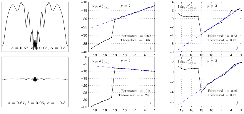
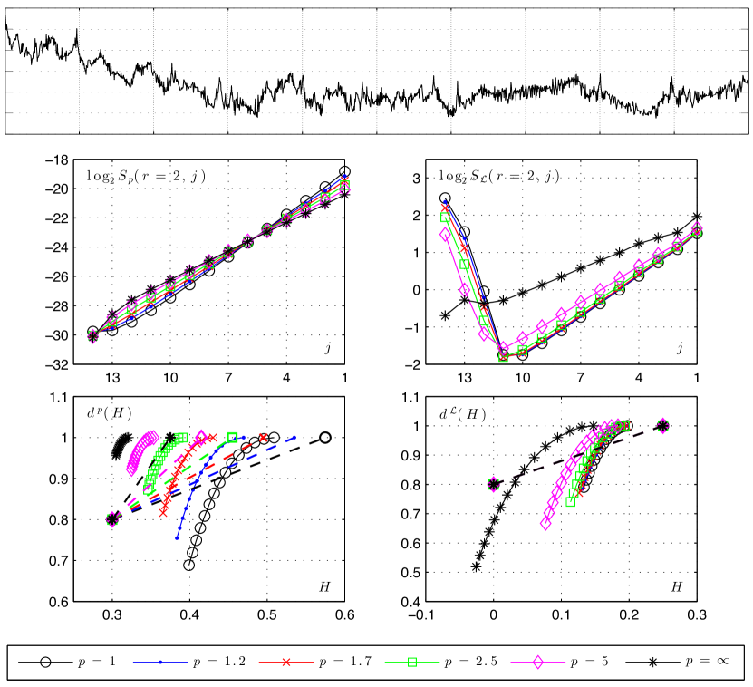
Numerical examples for the estimation of $d^{p}(H)$ and $d^{\mathcal{L}}(H)$ of a lacunary wavelet series are given in Figure 5. As predicted by theory, the numerical estimates of the $p$-exponent multifractal spectra are not invariant with $p$ but follow the evolution with $p$ of the theoretical spectra $d^{p}(H)$. The positions of the mode of the estimated spectra have a constant negative bias; yet, quantitatively, they very well reproduce the shift of the mode of the theoretical spectra to smaller values of $H$ for increasing $p$, revealing the lacunary nature of the function. A refined analysis is possible with the estimated lacunarity exponent multifractal spectrum $d^{\mathcal{L}}(H)$, which has been computed here for several values of $p$ for illustration purposes. The mode of the spectrum is estimated at $H\approx 0.2$ (instead of the theoretical $H=0.25$). This clearly indicates the existence of positive lacunarity exponents. While the estimates for small values of $p$ fall short of revealing the full support of the theoretical multifractal spectrum, they still enable one to identify a relatively large interval of positive lacunarity exponent values. The best estimate of $d^{\mathcal{L}}(H)$ is obtained for the canonical value $p=p_{0}=+\infty$ ($q=q_{0}=0$) in this example and produces a satisfactory concave envelope of the theoretical multifractal spectrum that provides clear evidence for ensembles of lacunary singularities with a range of positive exponents.

5. Concluding remarks

The analysis that we developed is based on the assumption that $p_{0}(f)>0$, or that $\eta_{f}(p)>0$ for $p$ small enough, so that $p$-exponents can be defined, at least, for $p\leq p_{0}$; we saw that this assumption allows us to deal with distributions of arbitrarily large order and, equivalently, to model pointwise singularities with arbitrarily large negative exponent. However, this does not imply that any tempered distribution satisfies these assumptions. Simple counterexamples are supplied by the Gaussian fractional noises $B_{{\alpha}}$ for ${\alpha}<0$ whose sample paths can be seen as fractional derivatives of order $\frac{1}{2}-{\alpha}$ of the sample paths of a Brownian motion on ${\mathbb{R}}$ (Gaussian white noise corresponds to ${\alpha}=-1/2$, in which case it is a derivative, in the sense of distributions, of Brownian motion). In [18] the wavelet and leader scaling functions are derived, and it is proved that $\eta_{B_{{\alpha}}}=-{\alpha}p$, hence always is negative. However, the following result shows that, as soon as the wavelet expansion of the data has some sparsity, then this phenomenon no more occurs, and $p_{0}$ is always strictly positive (note that this situation is quite common in practice since sparse wavelet expansions are often met in applications).

Definition 12.

A wavelet series $\sum_{j,k}c_{j,k}\psi_{j,k}$ is sparse if there exist $C>0$ and $\eta<1$ such that, on any interval $[l,l+1]$,

Cโ€‹aโ€‹rโ€‹dโ€‹{k:cj,kโ‰ 0}โ‰คCโ€‹2ฮทโ€‹j.๐ถ๐‘Ž๐‘Ÿ๐‘‘conditional-set๐‘˜subscript๐‘๐‘—๐‘˜0๐ถsuperscript2๐œ‚๐‘—Card\{k:\;c_{j,k}\neq 0\}\leq C2^{\eta j}.

Typical examples of sparse wavelet series are supplied by lacunary wavelet series or by the measures which satisfy (29). The following proposition implies that multifractal analysis based on $p$-exponents is always possible for data with a sparse wavelet expansion.

Proposition 5.1.

Let $f$ be a tempered distribution, which has a sparse wavelet expansion, then $\eta_{f}(p)>0$ for $p$ small enough, so that $p_{0}(f)>0.$

Proof: Since $f$ is a tempered distribution, it has a finite order, and thus it is a derivative of order $A$ of a continuous function. Therefore $f$ belongs to $C^{-A}({\mathbb{R}})$, so that

$$|c_{j,k}|\leq C2^{Aj}.$$

Using again compactly supported wavelets, the same argument as in the proof of Proposition 3.4 yields that there are at most $C2^{\eta j}$ nonvanishing wavelet coefficients at scale $j$; it follows that

$$2^{-j}\sum_{k}|c_{j,k}|^{p}\leq C2^{-j}2^{\eta j}2^{Apj}$$

so that $\eta_{f}(p)\geq 1-\eta-Ap$, and $\eta_{f}(p)>0$ for $p<(1-\eta)/A$.

References

  • [1] P. Abry, S. Jaffard, and H. Wendt. A bridge between geometric measure theory and signal processing: Multifractal analysis. In K. Grochenig, Y. Lyubarskii, and K. Seip, editors, Operator-Related Function Theory and Time-Frequency Analysis, The Abel Symposium 2012, pages 1โ€“56. Springer, 2015.
  • [2] P. Abry, H. Wendt, S. Jaffard, H. Helgason, P. Goncalves, E. Pereira, C. Gharib, P. Gaucherand, and M. Doret. Methodology for multifractal analysis of heart rate variability: From LF/HF ratio to wavelet leaders. In Nonlinear Dynamic Analysis of Biomedical Signals EMBC conference (IEEE Engineering in Medicine and Biology Conferences ) Buenos Aires, 2010.
  • [3] S. Abry, P. Jaffard and H. Wendt. Irregularities and scaling in signal and image processing: Multifractal analysis. Benoit Mandelbrot: A Life in Many Dimensions, M. Frame and N. Cohen, Eds., World Scientific publishing, pages 31โ€“116, 2015.
  • [4] A. Arneodo, E. Bacry, S. Jaffard, and J.-F. Muzy. Singularity spectrum of multifractal functions involving oscillating singularities. J. Four. Anal. Appli., 4:159โ€“174, 1998.
  • [5] J.M. Aubry and S. Jaffard. Random wavelet series. Communications in Mathematical Physics, 227(3):483โ€“514, 2002.
  • [6] B. Baraล„ski, K.and Bรกrรกny and J. Romanowska. On the dimension of the graph of the classical Weierstrass function. Advances in Mathematics, 265:32โ€“59, 2014.
  • [7] V. V. Beresnevitch and S. S. Velani. A mass transference principle and the Duffin-Schaeffer conjecture for Hausdorff measures. Annals of Mathematics, 164:971โ€“992, 2006.
  • [8] A.P. Calderon and A. Zygmund. Local properties of solutions of elliptic partial differential equations. Studia Math.,, 20:171โ€“223, 1961.
  • [9] A. Durand. Random wavelet series based on a tree-indexed Markov chain. Comm. Math. Phys., 283(2):451โ€“477, 2008.
  • [10] A. Fraysse. Regularity criteria of almost every function in a Sobolev space. Journal of Functional Analysis, 258:1806โ€“1821, 2010.
  • [11] S. Jaffard. Multifractal formalism for functions. SIAM J. of Math. Anal., 28(4):944โ€“998, 1997.
  • [12] S. Jaffard. On lacunary wavelet series. Annals of Applied Probability, 10(1):313โ€“329, 2000.
  • [13] S. Jaffard. Wavelet techniques in multifractal analysis. In Fractal Geometry and Applications: A Jubilee of Benoรฎt Mandelbrot, M. Lapidus and M. van Frankenhuijsen Eds., Proceedings of Symposia in Pure Mathematics, volume 72(2), pages 91โ€“152. AMS, 2004.
  • [14] S. Jaffard. Pointwise regularity associated with function spaces and multifractal analysis. Banach Center Pub. Vol. 72 Approximation and Probability, T. Figiel and A. Kamont, Eds., pages 93โ€“110, 2006.
  • [15] S. Jaffard. Wavelet techniques for pointwise regularity. Ann. Fac. Sci. Toul., 15(1):3โ€“33, 2006.
  • [16] S. Jaffard, P. Abry, and S.G. Roux. Function spaces vs. scaling functions: tools for image classification. Mathematical Image Processing (Springer Proceedings in Mathematics) M. Bergounioux ed., 5:1โ€“39, 2011.
  • [17] S. Jaffard, P. Abry, S.G. Roux, B. Vedel, and H. Wendt. The contribution of wavelets in multifractal analysis, pages 51โ€“98. Series in contemporary applied mathematics. World Scientific publishing, 2010.
  • [18] S. Jaffard, B. Lashermes, and P. Abry. Wavelet leaders in multifractal analysis. In Wavelet Analysis and Applications, T. Qian, M.I. Vai, X. Yuesheng, Eds., pages 219โ€“264, Basel, Switzerland, 2006. Birkhรคuser Verlag.
  • [19] S. Jaffard and C. Melot. Wavelet analysis of fractal boundaries. Communications in Mathematical Physics, 258(3):513โ€“565, 2005.
  • [20] S. Jaffard, C. Melot, R. Leonarduzzi, H. Wendt, S.G. Roux, M. E. Torres, and P. Abry. p-Exponent and p-Leaders, Part I: Negative pointwise regularity. 2015. in review.
  • [21] Stรฉphane Jaffard. Pointwise regularity criteria. C. R., Math., Acad. Sci. Paris, 339(11):757โ€“762, 2004.
  • [22] Y. Meyer. Ondelettes et Opรฉrateurs. Hermann, Paris, 1990. English translation, Wavelets and Operators, Cambridge University Press, 1992.
  • [23] G. Parisi and U. Frisch. Fully developed turbulence and intermittency. In M. Ghil, R. Benzi, and G. Parisi, editors, Turbulence and Predictability in Geophysical Fluid Dynamics and Climate Dynamics, Proc. of Int. School, page 84, Amsterdam, 1985. North-Holland.
  • [24] R.H. Riedi. Multifractal processes. In P. Doukhan, G. Oppenheim, and M.S. Taqqu, editors, Theory and applications of long range dependence, pages 625โ€“717. Birkhรคuser, 2003.
  • [25] D. Rockmore, J. Coddington, J. Elton, and Y. Wang. Multifractal analysis for Jackson Pollock. SPIE, pages 6810โ€“13, 2008.
  • [26] W. Stute. The oscillation behavior of empirical processes. Annals of Probability, 10:86โ€“107, 1982.
  • [27] H. Triebel. Fractal characteristics of measures; an approach via function spaces. Jour. Four. Anal. Applic., 9(4):411โ€“430, 2003.
  • [28] H. Wendt, S.G. Roux, P. Abry, and S. Jaffard. Wavelet leaders and bootstrap for multifractal analysis of images. Signal Proces., 89:1100โ€“1114, 2009.