Critical dynamics of the $k$-core pruning process

Abstract

We present the theory of the $k$-core pruning process (progressive removal of nodes with degree less than $k$) in uncorrelated random networks. We derive exact equations describing this process and the evolution of the network structure, and solve them numerically and, in the critical regime of the process, analytically. We show that the pruning process exhibits three different behaviors depending on whether the mean degree $\langle q\rangle$ of the initial network is above, equal to, or below the threshold $\langle q\rangle_{c}$ corresponding to the emergence of the giant $k$-core. We find that above the threshold the network relaxes exponentially to the $k$-core. The system manifests the phenomenon known as “critical slowing down”, as the relaxation time diverges when $\langle q\rangle$ tends to $\langle q\rangle_{c}$. At the threshold, the dynamics become critical characterized by a power-law relaxation ($\propto 1/t^{2}$). Below the threshold, a long-lasting transient process (a “plateau” stage) occurs. This transient process ends with a collapse in which the entire network disappears completely. The duration of the process diverges when $\langle q\rangle\rightarrow\langle q\rangle_{c}$. We show that the critical dynamics of the pruning are determined by branching processes of spreading damage. Clusters of nodes of degree exactly $k$ are the evolving substrate for these branching processes. Our theory completely describes this branching cascade of damage in uncorrelated networks by providing the time dependent distribution function of branching. These theoretical results are supported by our simulations of the $k$-core pruning in Erdős–Rényi graphs.

I Introduction

Pruning algorithms for networks provide an effective way to extract subgraphs distinguished by their structural properties, connectivity, robustness against failures and damaging, and other features Seidman (1983); Bollobás (1984); Łuczak (1991); Batagelj and Zaveršnik (2002); Dorogovtsev et al. (2006a); Buldyrev et al. (2010). In general pruning processes, parts of a network are progressively removed from it according to some rule. If the rule is simply random removal of nodes, we obtain ordinary percolation Albert and Barabási (2002); Newman (2003); Dorogovtsev et al. (2008), but in general we are interested in more complex pruning rules. The parts removed may be nodes Seidman (1983); Pittel et al. (1996); Dorogovtsev et al. (2006a), clusters Bauer and Golinelli (2001), finite connected components in interdependent and multiplex networks Buldyrev et al. (2010); Zhou et al. (2012, 2014); Son et al. (2012), etc. Despite the wide variety of pruning processes, many of them demonstrate similar behaviors, such as discontinuous hybrid phase transitions. The $k$-core pruning as the simplest pruning process of this kind, stands as a paradigm for all such pruning processes, so its theory should help to understand the behavior of these pruning algorithms in general. The $k$-core is the network subgraph in which all nodes have degree at least $k$ Bollobás (1984). Since $k$-cores represent the densest parts of networks, they play an important role in understanding the structure and dynamics of complex network systems Dorogovtsev et al. (2008). The standard algorithm for finding the $k$-core of a network employs the following pruning process: at each step remove all nodes of degree less than $k$. This removal decreases the degrees of remaining nodes, some of which will become smaller than $k$. So, the pruning is repeated until either the $k$-core remains or the network disappears Pittel et al. (1996).

Previous investigations have mainly focused on the final result of the $k$-core pruning process, namely the $k$-core. These were the studies which showed that $k$-core percolation is a hybrid phase transition, combining discontinuity and a critical singularity, in contrast to ordinary percolation (continuous phase transition) Dorogovtsev et al. (2006a, 2008, b). However, associating the number of steps in the pruning process with time $t$ reveals a process exhibiting complex dynamics above, below, and at the $k$-core percolation threshold. Understanding the $k$-core pruning process and accompanying structural changes can shed light on such physical phenomena as the jamming transition, the rigidity percolation, and glassy dynamics Birolli (2007). Furthermore, the $k$-core pruning process is one of the simplest examples of dynamic processes associated with hybrid phase transitions, sharing, for example, some common properties with cascade failures in interdependent networks that have recently received significant attention in the literature Buldyrev et al. (2010); Zhou et al. (2013); Grassberger (2015); Zhou et al. (2012, 2014); Boccaletti et al. (2014); Kivelä et al. (2014); Baxter et al. (2012).

In this paper we develop the detailed theory of the $k$-core pruning process in uncorrelated, sparse random networks, describing the temporal evolution of the networks structure, the spreading of damage over the network, and critical phenomena in this process. We show that near the threshold value of the mean degree, $\langle q\rangle_{c}$, corresponding to the emergence of the giant $k$-core, this cascade of removals of nodes is a branching process with the mean branching coefficient close to $1$. Our theory describes this process completely providing the full time dependent distribution of branching from the beginning until the end of the pruning. We indicate that the clusters of nodes of degree $k$ (so-called “corona clusters”), evolving due to the pruning, provide the substrate for the branching processes. Near the threshold we find three different behaviors depending on whether the mean degree $\langle q\rangle$ of the initial network is above, equal to, or below the threshold. First, we demonstrate that above the threshold, the network relaxes exponentially to the steady $k$-core. The relaxation time diverges when $\langle q\rangle$ tends to $\langle q\rangle_{c}$, manifesting a phenomenon known as “critical slowing down”. Second, at the critical point, $\langle q\rangle=\langle q\rangle_{c}$, the dynamics is critical, characterizied by a power-law relaxation with $1/t^{2}$ dependence. Third, below the threshold, a long-lasting transient process (a “plateau” stage) occurs. This transient process ends with a collapse in which the entire network disappears. We find that the duration of the process diverges when $\langle q\rangle$ approaches $\langle q\rangle_{c}$. Our theory is supported by numerical calculations for Erdős–Rényi graphs and by simulations of the pruning process in these random graphs.

In Sec. II we derive the exact equations describing the evolution of the network structure during the pruning process enabling us to obtain the time dependent degree distribution $P(q,t)$ and the branching probability distribution ${\cal P}(n,t)$ at all times. Close to the critical point, the probability that different branches of the process cross each other is negiligibly small. We show that in this region, our equations take a simple form for analytical treatment. Section III explores the three regimes of the pruning process below, at, and above the threshold. Section IV describes the statistics of the branching process. A relationship with dynamical systems close to a saddle-point bifurcation and details of calculations are given in the appendices.

II Evolution equations

To study the $k$-core pruning process, let us consider as a representative case an infinite uncorrelated sparse random network, which is completely defined by its degree distribution $P(q)$. In this case, we can write exact equations for the evolution of the degree distribution. Let $P(q,t)$ be the proportion of vertices having degree $q$ at time $t$, with the initial condition $P(q,0)=P(q)$. At each time $t=1,2,3,...$, all vertices with degree $q$ less than $k$ are pruned by having all edges connected to them removed from the network. The probability $P(0,t)$ thus tracks the number of vertices pruned so far.

II.1 Exact evolution equations

The removal of edges from pruned vertices means that some non-pruned vertices will also lose edges, changing the degree distribution of the remaining network. Let $r_{t}$ be the probability that, upon following a randomly chosen edge within the network existing at time $t$, we arrive at a vertex with degree less than $k$:

$$r_{t}=\frac{1}{\langle q\rangle_{t}}\sum_{q<k}qP(q,t).$$ (1)

Such an edge will be removed in the subsequent step. Here $\langle q\rangle_{t}$ is the mean degree of the surviving network at time $t$,

$$\langle q\rangle_{t}=\sum_{q}qP(q,t).$$ (2)

The probability that a vertex of degree $q^{\prime}\geq k$ at time $t$ has $q$ surviving edges at time $t+1$ is then $\binom{q^{\prime}}{q}(1{-}r_{t})^{q}r_{t}^{q^{\prime}-q}$. A vertex of degree $q^{\prime}<k$ at time $t$ will of course have degree zero at time $t+1$. Summing over all $q^{\prime}$, the degree distribution then evolves as follows:

$$P(q,t+1)=\sum_{q^{\prime}\geq\max\{q,k\}}P(q^{\prime},t)\binom{q^{\prime}}{q}(1-r_{t})^{q}r_{t}^{q^{\prime}-q}$$ (3)

for $q>0$ while the fraction of pruned nodes evolves according to

$$P(0,t+1)=\sum_{q^{\prime}<k}P(q^{\prime},t),$$ (4)

where the sum includes $q^{\prime}=0$. The uncorrelated nature of the network ensures that Eqs. (1)–(4) completely define the evolution of the network at all times. Note that another approach for the pruning process which, however, does not consider the evolution of the network structure, was proposed in Iwata and Sasa (2009).

Figure 1: (Color online) A snapshot of the branching process of propagation of node pruning in a small part of the network of $10^{5}$ nodes during the plateau stage ($\langle q\rangle<\langle q\rangle_{c}$) of the $k$-core pruning process for $k=3$. The node labelled $0$ is pruned, causing the corona nodes (i.e., nodes with degree $3$) labelled $1$ to lose edges. These two nodes are pruned in the next step, and so on, with further corona nodes removed in subsequent steps according to the numbered order. Red and white circles represent the nearest neighboring nodes of degree $4$ and greater than $4$, respectively, that survive because their degrees exceed $3$. The red nodes after this pruning become of degree $3$. They augment other corona clusters, which may then be pruned at a later time.

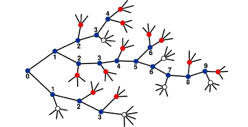
To understand the spreading of damage through the network as the pruning process evolves, we introduce the probability $s_{t}$. This is the probability that, following an edge at time $t$, we reach a vertex that has degree at least $k$ at time $t$, but will have no more than $k-1$ other surviving edges at time $t+1$ (not counting the edge through which we reached the vertex). This means that if the edge we are following is removed at time $t$, the vertex that it leads to will be removed at time $t+1$. To calculate $s_{t}$, we sum over probabilities that all but $l$ of the $q-1$ outgoing edges of a vertex of degree $q$ (i.e. $q-1-l$ edges) are lost at time $t$ (each one with probability $r_{t}$) with $l$ equal to at most $k-1$. A second summation is then performed over all possible degrees $q\geq k$:

$$s_{t}=\frac{1}{\langle q\rangle_{t}}\sum_{q\geq k}qP(q,t)\sum_{l=0}^{k-1}\binom{q-1}{l}r_{t}^{q-1-l}(1-r_{t})^{l}.$$ (5)

The probability $\mathcal{P}(n,t)$ that a vertex removed at time $t$ has $n$ neighbors that will be removed at time $t+1$ is then

$$\mathcal{P}(n,t)=\frac{\sum_{q=n}^{k-1}P(q,t)\binom{q}{n}s_{t}^{n}(1-s_{t})^{q-n}}{\sum_{q=1}^{k-1}P(q,t)}.$$ (6)

This function describes the branching of spreading damage. The mean branching is

$$b_{t}=\sum_{n=0}^{k-1}n\mathcal{P}(n,t)=s_{t}\frac{\sum_{q=1}^{k-1}qP(q,t)}{\sum_{q=1}^{k-1}P(q,t)}.$$ (7)

II.2 Non-crossing approximation

Unfortunately, it is difficult to study analytically Eqs. (1)–(4). In this subsection we develop an approximate approach providing the asymptotic description of the pruning process at large times near the critical point.

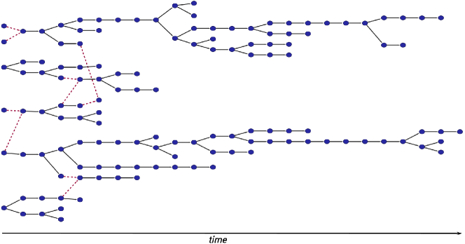
When the probability $r_{t}$ is very small, the pruning can then be considered as a branching process. The probability that a vertex loses two neighbors in a single step is negligible, in other words, the probability that two or more branching trees meet at a vertex is negligible. The process then evolves with independent branching trees spreading simultaneously over the network. An example of such non-crossing branchings observed in simulations is shown in Fig. 1. If crossings are negligible, then the fraction of vertices of degree $q<k-1$ is also negligible and only vertices of degree $q\geq k-1$ must be taken into account. This is the main assumption of the “non-crossing” approximation. This approximation is supported by our numerical solution of Eqs. (1)–(4) and simulations which show that the probability of crossings between branches are negligible and $P(k-1,t)\gg P(k-2,t)\gg\dots P(1,t)$ already after a short initial period (see the next sections). Applying the non-crossing approximation to Eq. (5), we find that $s_{t}$ becomes simply the probability that, following an edge at time $t$, we encounter a vertex of degree $k$.

$$s_{t}\approx\frac{kP(k,t)}{\langle q\rangle_{t}}.$$ (8)

Furthermore, the probability $r_{t}$, Eq. (1), and the mean branching $b_{t}$, Eq. (7), take the simple forms,

$$r_{t}\approx\frac{(k-1)P(k-1,t)}{\langle q\rangle_{t}},$$ (9)

$$b_{t}\approx\frac{(k-1)kP(k,t)}{\langle q\rangle_{t}}.$$ (10)

So $r_{t}$ is simply the probability that, following an edge at time $t$, we encounter a vertex of degree $k-1$. The evolution equation (3) is also simplified. The following set of equations determines the evolution of the degree distribution during the $k$-core pruning process:

$$\!\!\!\!\!\!\!\!P(q,t{+}1){=}P(q,t){-}r_{t}qP(q,t){+}r_{t}(q{+}1)P(q{+}1,t),$$ (11)

$$\!\!\!\!\!\!\!\!P(k-1,t+1)=r_{t}kP(k,t),$$ (12)

$$\!\!\!\!\!\!\!\!P(0,t+1)=P(0,t)+P(k-1,t),$$ (13)

$$\!\!\!\!\!\!\!\!\langle q\rangle_{t}=(k-1)P(k-1,t)+\sum_{q\geq k}qP(q,t),$$ (14)

where $q\geq k$. The negative term in Eq. (11) corresponds to the reduction in $P(q,t)$ due to vertices of degree $q$ losing with the probability $qr_{t}$ a single edge, while the positive term (last term) corresponds to an increase in $P(q,t)$ due to vertices of degree $q+1$ losing an edge with the probability $(q+1)r_{t}$ and so ending up with degree $q$.

Using Eq. (10), we rewrite Eq. (12) as follows,

$$P(k-1,t+1)=b_{t}P(k-1,t).$$ (15)

Equations (12) and (15) show that the removal of a vertex of degree $k{-}1$ at time $t$ triggers in the next step the removal of all corona vertices attached to it since they will lose one edge and will have degree $k{-}1$. On average, the number of these corona vertices is the mean branching $b_{t}$. In uncorrelated networks, Eqs. (11)–(14) describe the non-crossing branching processes of spreading damage (see Appendices B and C). They show that vertices of degree $k$ (“corona” vertices) are crucial for spreading damage. In the case $\langle q\rangle\geq\langle q\rangle_{c}$ at large times, $t\gg 1$, crossings are negligible and these equations are asymptotically exact. Equations (11)–(14) are not valid when there are numerous crossings between branching processes. Such crossings are abundant both at the initial stage of the pruning process and at the end of the “plateau” stage when the network collapses. In this case, the exact Eqs.(1)–(4) must be used. Branching processes are discussed in detail below in Sec. IV.

III Three regimes of the pruning process

As a representative example of the pruning process, we solved Eqs. (1)–(4) numerically for Erdős-Rényi networks (Poisson degree distributions) using the initial mean degree $\langle q\rangle$ as a control parameter. We solved the equations for $k=3$ and $k=5$. The $3$-core appears with a hybrid transition at $\langle q\rangle_{c}\approx 3.35091887$, while for the $5$-core, $\langle q\rangle_{c}\approx 6.7992755$. We also performed simulations of the pruning process in the networks. We found that for any $k\geq 3$, the dynamics of the pruning process can be divided into three different regimes: $\langle q\rangle<\langle q\rangle_{c}$, $\langle q\rangle>\langle q\rangle_{c}$, and $\langle q\rangle=\langle q\rangle_{c}$.

III.1 Pruning process below $\langle q\rangle_{c}$

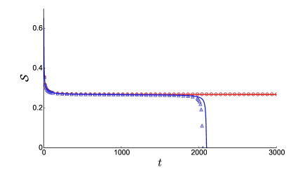
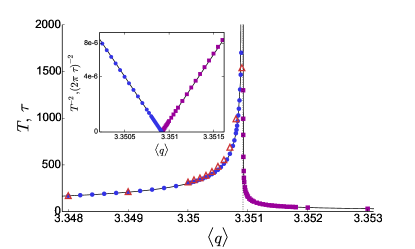
Below $\langle q\rangle_{c}$, the pruning process ends in a finite time (number of steps) with the complete destruction of the infinite network. Rapid pruning of vertices at early times soon slows down and the system enters a “plateau” stage in which the rate of removal of vertices is very slow. Finally, this transient process ends with a collapse in which the entire network disappears, as can be seen in Fig. 2 which displays the temporal dependence of the network size $\mathcal{S}$. The duration of the entire process, from beginning until final collapse, diverges as the inverse square root of the distance from the critical point,

$$T=A_{\text{below}}/\sqrt{\langle q\rangle_{c}-\langle q\rangle},$$ (16)

as shown in Fig. 3. The time $T$ is mainly determined by the duration of the “plateau” stage. Note that the inverse square-root scaling law is a general feature of non-linear dynamic systems that are close to a saddle-node bifurcation Strogatz and Westervelt (1989); Strogatz (1994). In such systems, the long-lasting transient process is caused by a bottleneck region (the ghost) that exists in phase space when the system is close to a saddle-node bifurcation or the limiting point of metastable states in the case of the first order phase transitions (see a simple model in Appendix A). The nature of the bottleneck effect in the $k$-core pruning process is discussed in Sec. IV.

Figure 2: (Color online) Size $\mathcal{S}$ of the Erdős-Rényi network vs time $t$ during the pruning process for $k=3$ in two cases: (i) below the threshold $\langle q\rangle_{c}$, the system passes through a long “plateau” stage before a final collapse. Shown are numerical calculations for mean degree $\langle q\rangle=3.3509$ (blue solid line) and simulations (triangles) for a network of $10^{8}$ vertices showing similar total time. (ii) Above $\langle q\rangle_{c}$, the system relaxes to a finite size, numerical solution for $\langle q\rangle=3.35092$ (red solid line) and simulations (circles).

III.2 Pruning process above $\langle q\rangle_{c}$

Above $\langle q\rangle_{c}$ a finite fraction of the network remains indefinitely and the network relaxes to the steady $k$-core only in the infinite time limit (see Fig. 2). In this regime, according to the numerical solution of Eqs. (1)–(4) and simulations, the relaxation to the steady state is exponential. Instead of measuring the total time, we characterize the time scale of the pruning process by measuring the relaxation time $\tau$, where:

$$P(k-1,t)\propto e^{-t/\tau}.$$ (17)

The relaxation time $\tau$ diverges as the inverse square root of the distance from the critical point, as seen in Fig. 3,

$$\tau=A_{\text{above}}/\sqrt{\langle q\rangle_{c}-\langle q\rangle}.$$ (18)

We examine the origin of this scaling in more detail in the next Sec. IV.2, using the non-crossing approximation.

The divergence of $\tau$ manifests the phenomenon known as critical slowing down. Furthermore, comparing the amplitudes $A_{\text{below}}$ and $A_{\text{above}}$ of the square-root singularities below and above the transition, we find their ratio to be $A_{\text{below}}/A_{\text{above}}=9.133/1.452=6.29$ for $k=3$ and $8.44/1.34=6.28$ for $k=5$, in agreement with the ratio $2\pi$ expected for general transitions of this kind, see Appendix A.

Figure 3: (Color online) Characteristic times associated with the $k$-core pruning process for $k=3$ on an Erdős-Rényi network. Circles show the duration $T$ of the entire pruning process below $\langle q\rangle_{c}$. Squares show the relaxation time constant $\tau$ above $\langle q\rangle_{c}$. Fitted square root scaling for $T$ and $\tau$ are shown by black solid lines. The critical point $\langle q\rangle_{c}$ is marked by a vertical dotted line. Completion times for a simulated network of $10^{8}$ vertices are also shown below $\langle q\rangle_{c}$ (triangles). In the inset, the inverse squares of $T$ and $\tau$ (also scaled by $2\pi$) are shown, demonstrating the inverse square dependence on the distance from the critical point.

Figure 4: (Color online) Time evolution of the network degree distribution during the $k$-core pruning process, for an Erdős-Rényi network with $k=3$. Each line shows $P(q,t)$ for a different value of $q$, in order from top to bottom, $q=3,4,5,2,1$, as labelled. (left) Initial mean degree $\langle q\rangle=3.3509$, (right) initial mean degree $\langle q\rangle=3.35092$. Also shown are traces from simulation runs for an Erdős-Rényi network with $N=10^{8}$ vertices and mean degree $3.3511$ (left) and $3.35111$ (right). Note that the critical point for a particular realisation is a stochastic quantity, so the mean degrees for matching theory and simulation are not necessarily equal. Theoretical curves were chosen to be near the critical point and to have a similar total time.

Figure 5: Decay of $P(k-1)$ on a log-log scale for several values of $\langle q\rangle$ close to $\langle q\rangle_{c}$. Exactly at the critical point, the decay follows a power law with exponent $-2$. (For clarity, the final collapse of $P(k-1)$ for curves below the critical point is not shown.) Curves are plotted for the Erdős–Rényi graphs with the mean degree values (labelled $1$ to $6$) $3.350905$, $3.35091$, $3.350915$, which are below $q_{c}$, $3.35091887$ (very close to $q_{c}$), and $3.35092$, $3.350925$, which are above $q_{c}$. Dashed line is a power-law decay with exponent $-2$.

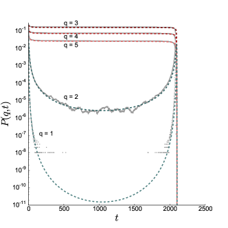
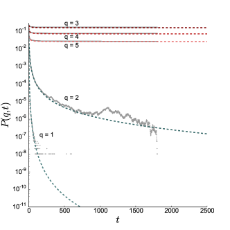
In Fig. 4 we show the evolution of the degree distribution just above and just below $\langle q\rangle_{c}$. Near the critical mean degree the initial evolution of the degree distribution $P(q,t)$ both above and below the critical point is similar, namely, there is a sharp initial decrease of $P(q,t)$ for nonzero $q$. Below $\langle q\rangle_{c}$, however, the network finally collapses completely, while above the critical point, the $k$-core survives forever. The theoretical results agree well with simulation.

III.3 Critical pruning process

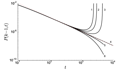
Solving Eqs. (1)–(4) numerically for Erdős-Rényi networks, we find that exactly at the critical point, $\langle q\rangle_{c}$, the relaxation is much slower, with $P(k-1,t)$ decaying as a power law,

$$P(k-1,t)\propto\frac{1}{t^{\sigma}}.$$ (19)

as can be seen in Fig. 5. For $k=3$ we measured the exponent $\sigma=-1.993$ at $\langle q\rangle=3.35091887$, suggesting that the exponent is $-2$. Note that in a simple model of a particle moving in a one-dimensional potential in Appendix A the corresponding critical exponent is $-1$ [see Eq. (32)]. We explain the power-law behavior, Eq. (19), in Appendix B by solving Eqs. (38)–(41) within the non-crossing approximation. This approach gives the exact value $\sigma=2$.

Figure 6: (Color online) Example of the pruning process from time $t=10$ till 34 in a small part of the Erdős-Rényi network with $10^{5}$ nodes. Time progresses from left to right in the tree. Blue circles represent vertices removed at a given time step. Their removal results in the removal of vertices on the right, and so on. Crossings (dashed lines) between the branching processes are abundant at the beginning of the pruning process. They appear rarely after a short initial period. Typical trees of medium size are shown. Much longer and much shorter trees also occur.

Figure 7: (Color online) Evolution of the branching distribution $\mathcal{P}(n,t)$ below (left) and above (right) the critical point for $k=3$. Solid and dashed curves are theoretical curves from Eq. (6) for $n$ as labelled, for $\langle q\rangle=3.3509$ (left) and $\langle q\rangle=3.35092$ (right). Points are measured from simulation of an Erdős-Rényi network of $10^{8}$ nodes, at $\langle q\rangle=3.3511$ (left) and $3.35111$ (right), being just below and just above the critical mean degree for that network.

Figure 8: (Color online) Evolution of the mean branching ratio $b_{t}$ below (left) and above (right) the critical point for $k=3$. Dashed curves are calculated using Eq. (10), points are from simulations. Parameters used and simulation realisations are the same as in Fig. 7.

Figure 9: (Color online) Phase diagram for the $k$-core pruning process in $\langle q\rangle-t$ plane. The vertical line represent the critical point $\langle q\rangle=\langle q\rangle_{c}$ ($k=3$ for this figure). In region II at $\langle q\rangle>\langle q\rangle_{c}$, the pruning process reduces the network to the giant $k$-core as time approaches infinity. Only finite corona clusters are present in region II. A giant corona cluster is present in region III. The mean branching is $1$ on the border between regions II and III. The mean branching is below $1$ in region II and larger than $1$ in region III. The network collapses at times on the upper boundary of region III so there is no network in region I.

IV Branching processes of pruning

In this section, to understand the nature of the critical dynamics of the pruning process, we study the spreading of damage through the network and the structural changes during this process. The probability $\mathcal{P}(n,t)$ of the branching process is given by Eq. (6) that takes a simple form within the non-crossing approximation,

$$\mathcal{P}(n,t)=\binom{k-1}{n}s_{t}^{n}(1-s_{t})^{k-1-n}.$$ (20)

Since the parameter $s_{t}$ given by Eq. (8) is the probability to encounter a vertex of degree $k$ (corona vertex), the probability Eq. (20) is precisely the probability that following an edge we arrive at a corona vertex which has $n$ corona vertices at the ends of emanating edges Goltsev et al. (2006). It is important to note that as the network evolves according Eqs. (1)–(4) during the $k$-core pruning process, so do the corona clusters and hence their size distribution. Since the probability $s_{t}$ and, therefore, the probability $\mathcal{P}(n,t)$ of the branching process depend on time, the size distribution of branches of removed vertices is therefore related but not equal to the instantaneous size distribution of corona clusters (see the following subsection).

IV.1 Branching processes at $\langle q\rangle<\langle q\rangle_{c}$

The numerical solution of Eqs. (1)–(4) and simulation show that, in the case $\langle q\rangle<\langle q\rangle_{c}$ during the plateau stage, the pruning process develops as a branching process, as described in Sec. II.2. The branching process of removals evolves in agreement with Eqs. (8)–(15). Examples of typical pruning trees are illustrated in Fig. 6 for $k=3$. The figure shows that crossings between the branching trees are only abundant at the beginning of the pruning process and are rare in the plateau stage. The crossings also are abundant at the end of the plateau stage, signaling a collapse in which the entire network disappears.

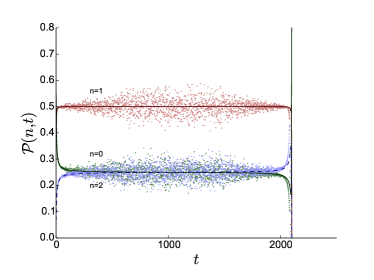
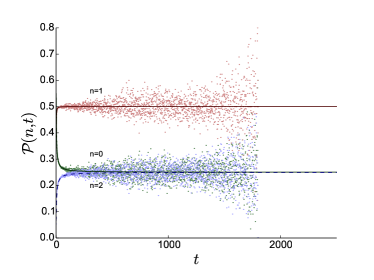
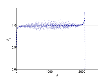
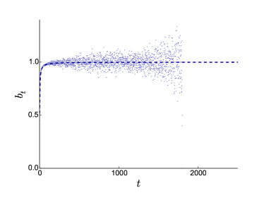
The full branching distribution, given by Eq. (6) is shown in Fig. 7. It is similar both above and below the transition, and barely changes throughout most of the pruning process. In the figure we also show the branching distribution observed in simulations. The agreement with theory is good, however there are noticeable finite size fluctuations, which are largest when the pruning process is slowest: this occurs in the middle of the plateau period. In contrast to this behavior, fluctuations in the case $\langle q\rangle\geq\langle q\rangle_{c}$ are enhanced with increasing time (see Fig. 7). Critical behavior of fluctuations is a common property of systems approaching the critical point of a continuous phase transition, or the limiting point of the metastable states of a first-order phase transition, however, discussion of these phenomena is beyond the scope of the present paper.

In the early part of the plateau, $P(k-1,t)$ decreases, reaching a minimum in the middle of the plateau stage, at $t=t_{m}$. From Eq. (39) this corresponds to the point when $b_{t}$ reaches $1$. A Taylor expansion around this point (see Appendix C) gives the temporal behavior of $P(k-1,t)$ in the plateau stage

$$P(k{-}1,t)=P(k-1,t_{m})\Bigl{[}1+\frac{1}{2}\Bigl{(}\frac{t}{t_{m}}-1\Bigr{)}^{2}C_{p}+\dots\Bigr{]},$$ (21)

The corresponding equation for $b_{t}$ is

$$b_{t}\approx 1+\Bigl{(}1-\frac{t}{t_{m}}\Bigr{)}C_{b},$$ (22)

Our analysis of the plateau stage in Appendix C shows that $C_{b}\sim 1/T\propto\sqrt{\langle q\rangle_{c}-\langle q\rangle}\ll 1$. This analytical result agrees with our observation from the numerical solutions. The mean branching $b_{t}$, Eq. (7), is slightly below $1$ in the beginning of the plateau stage. As time increases, $b_{t}$ tends to increase, as pruning of vertices decreases the mean degree of the network. The mean branching reaches $1$ at $t_{m}$ as required, then continues to increase, with an accelerating rate of pruning, until the network finally collapses rapidly, as seen on the left in Fig. 8. We observe from numerical solution of the exact Eqs. (1)–(4), and from simulations, that the minimum occurs in the middle of the plateau stage, i.e. $t_{m}=T/2$, see Fig. 4. The numerical solution of exact Eqs. (1)–(4) shows that the coefficient $C_{p}$ is of order 1. Using this result and Eq. (51) in Appendix C, we find a relationship between $P(k-1,t_{m})$ and the plateau duration $T$,

$$P(k-1,t_{m})\sim\frac{1}{T^{2}}\propto\langle q\rangle_{c}-\langle q\rangle.$$ (23)

The instantaneous size distribution $\Pi(S,t)$ of finite corona clusters can be found directly from the degree distribution $P(q,t)$ at every time $t$:

$$\Pi(S,t)=CS^{-3/2}e^{-S/S^{*}(t)}$$ (24)

where $S^{*}(t)\rightarrow\infty$ at the critical point of the emergence of a giant corona cluster. According to Goltsev et al. (2006), a giant connected cluster of corona vertices is present when

$$b_{t}=\frac{(k-1)kP(k,t)}{\langle q\rangle_{t}}\geq 1.$$ (25)

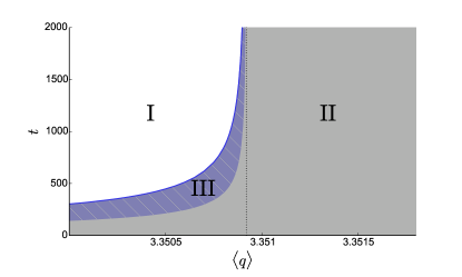
In the case of $k=3$, we have $S^{*}(t)=-1/\ln[4s_{t}(1-s_{t})]$ where $s_{t}=3P(3,t)/\langle q\rangle_{t}$ according to Eq. (8) Goltsev et al. (2006). In Appendix C we show that a giant corona cluster appears continuously at the same time $t_{m}$ when the fraction $P(k-1,t)$ of $k-1$ nodes achieves a minimum. Such a giant corona cluster will be consumed by the pruning process, guaranteeing the collapse of the whole network in finite time. A similar continuous emergence of a giant subgraph prone to failure was recently observed in interdependent networks in Ref. Zhou et al. (2014). The left side of Eq. (25) is identical to Eq. (10), so the border of the region where a giant corona cluster appears is at the point where the mean branching of the pruning process equals 1. The region in the $\langle q\rangle-t$ plane where the giant corona cluster is present is marked in Fig. 9 as region III. Note that a giant corona cluster only appears below $\langle q\rangle_{c}$ in the plateau stage. At $\langle q\rangle=\langle q\rangle_{c}$, at any time $t$ there are only finite corona clusters. When $t\to\infty$, the size distribution of corona clusters tends to the power law function Eq. (24), corresponding to the critical point of the emergence of a giant corona cluster. Above $\langle q\rangle_{c}$, there are only finite corona clusters at any time.

IV.2 Branching processes at $\langle q\rangle>\langle q\rangle_{c}$

Above the transition point, with increasing time the degree distribution $P(q,t)$ tends to the steady distribution $P_{k}(q)$ with mean degree $\langle q\rangle_{k}=\sum_{q\geq k}qP_{k}(q)$ while $P(k-1,t)\rightarrow 0$. In turn, the mean branching $b_{t}$ saturates at a constant value $b_{k}$ less than 1 (see the right side of Fig. 8). If $\langle q\rangle$ is close to $\langle q\rangle_{c}$, $1-k(k-1)P_{k}(k)/\langle q\rangle_{k}\approx B\sqrt{\langle q\rangle_{c}-\langle q\rangle}$ where $B$ is a constant Goltsev et al. (2006), and using Eq. (10) we have $b_{k}\approx 1-B\sqrt{\langle q\rangle_{c}-\langle q\rangle}$. Substituting the constant $b_{k}$ for $b_{t}=k(k-1)P_{k}(k,t)/\langle q\rangle_{t}$ in Eq. (39) in Appendix B, and solving, we find an exponential decay of $P(k-1,t)$, Eq. (17), and a relationship between the relaxation time $\tau$ and the branching coefficient $b_{k}$,

$$b_{k}=1-\tau^{-1}.$$ (26)

Therefore,

$$\tau^{-1}=1-k(k-1)P_{k}(k)/\langle q\rangle_{k}\approx B\sqrt{\langle q\rangle_{c}-\langle q\rangle}$$ (27)

in agreement with the numerical solution Eq. (18). The pruning process only evolves within finite corona clusters, and the network survives at any time $t$ (the region II in Fig. 9) approaching the steady $k$-core as time approaches infinity.

IV.3 Critical branching process

Exactly at the critical point, $\langle q\rangle=\langle q\rangle_{c}$, the branching $b_{t}$ comes arbitrarily close to 1, but only reaches that value in the infinite time limit. The leading term in $1-b_{t}$ is a monotonically decreasing function of $t$. Solving Eqs. (38)–(39) in Appendix B, we find that the function $P(k-1,t)$ has power-law behavior, Eq. (19), with critical exponent $\sigma=2$. This behavior corresponds to the mean branching $b_{t}$ increasing as

$$b_{t}=1-2/t+O(1/t^{2}).$$ (28)

This kind of time dependence of the mean branching is known to lead to the avalanche lifetime distribution $L(\mathcal{T})\propto\mathcal{T}^{-2}$ Harris (1989) found in various models (see, for example, Zapperi et al. (1995); Sethna et al. (2001)) and real systems (for example, in the brain Beggs and Plenz (2003)). This suggests that the power-law relaxation Eq. (19) and the avalanche lifetime distribution have the same origin.

Since the mean branching $b_{t}=(k-1)s_{t}$ tends to 1 when $t\rightarrow\infty$, we have $s_{t}\rightarrow 1/(k-1)$. Equation (20) gives the following exact result:

$$\mathcal{P}(n,\infty)=\binom{k-1}{n}\frac{(k-2)^{k-1-n}}{(k-1)^{k-1}}.$$ (29)

In the case of $k=3$, we obtain $\mathcal{P}(0,\infty)=\mathcal{P}(2,\infty)=1/4$ and $\mathcal{P}(1,\infty)=1/2$. These values agree with results obtained by our simulations and numerical solutions that are displayed in Fig. 7.

V Discussions and Conclusions

In this paper we have developed the theory of the $k$-core pruning process in uncorrelated, sparse random networks. Employing the numerical solution of the exact evolution equations, Eqs. (1)–(4), an asymptotic analysis, and simulations in Erdős-Rényi graphs, we revealed that this process demonstrates three different kinds of critical behavior depending on whether the mean degree $\langle q\rangle$ of the initial network is above, equal to, or below the critical point, $\langle q\rangle_{c}$, corresponding to the emergence of the giant $k$-core. We found that above the critical point, at large times the network relaxes exponentially to the steady $k$-core. At the critical point, $\langle q\rangle=\langle q\rangle_{c}$, the dynamics is critical and it is described by a power law with respect to time ($\propto 1/t^{2}$). Below the critical point, the pruning eliminates an infinite network in a finite time. The duration of the transient process diverges when $\langle q\rangle$ tends to $\langle q\rangle_{c}$ from below.

We found mechanisms for these critical phenomena. Studying the structure of paths along which damage is spreading in the network, we found that the damage spreading is a branching process. Our analysis showed that it is the evolving clusters of nodes of degree $k$ (“corona clusters”) that provide the substrate for the branching process. Indeed, if a vertex of degree $k$ loses an edge and is removed, then this removal triggers a removal of all corona vertices, one by one, which belong to the same corona cluster. Using analytical methods and simulation, we showed that the pruning can be considered as a branching process that begins after a short initial period of rapid network change. During this process, independent branching trees develop with branching ratio close to $1$. The temporal behavior of the mean branching plays a crucial role in the branching process and slowdown of the $k$-core pruning dynamics at the critical point and during the plateau stage. To understand the branching process it is important to note that corona clusters evolve in time. When damage propagates over the network, on one hand, it removes corona nodes, but on the other hand, it decreases the degrees of neighboring nodes, producing new corona vertices and thus increasing size of other corona clusters, which can be pruned at a later time. Due to this, the branching probability becomes time dependent. The mean branching is close to $1$ during the whole plateau stage, below $\langle q\rangle_{c}$. At the beginning of the stage the mean branching is a little bit smaller than $1$, and slowly increases with time. It reaches the value $1$ approximately at the middle of this stage and then continues to increase. At this point a giant corona cluster is formed providing a substrate for the complete collapse of the network at the end of the plateau stage. Exactly at the critical point, the mean branching comes arbitrarily close to $1$, but never reaches it at any finite time. This leads to a powerlaw decay in the fraction of nodes of degree $k-1$. The branching trees of pruning become arbitrarily long, but a giant corona cluster is never formed, until $t\to\infty$. Finally, we found that above the critical point $\langle q\rangle_{c}$, the mean branching saturates at a constant value less than 1. In this case, mean size of branches is finite and relaxation to the steady $k$-core follows an exponential law.

The $k$-core pruning process in sparse, uncorrelated random complex networks is a representative model of dynamics in complex systems undergoing hybrid phase transitions. We have solved this model and have developed the complete description of critical dynamical phenomena including the long-lasting transient process, critical relaxation, and critical slowing down. We suggest that our results could be useful for understanding similar collective phenomena that occur in other complex systems near discontinuous (hybrid and first-order) phase transitions.

VI Acknowledgements

This work is funded by FEDER funds through the COMPETE 2020 Programme and National Funds through FCT - Portuguese Foundation for Science and Technology under the project UID/CTM/50025/2013. This work was partially supported by the FET proactive IP project MULTIPLEX 317532, the FCT project EXPL/FIS-NAN/1275/2013, and the project “New Strategies Applied to Neuropathological Disorders” (CENTRO-07-ST24-FEDER-002034) cofunded by QREN and EU. KEL was supported by the FCT Grant No. SFRH/ BPD/ 71883/2010. GJB was supported by the FCT grant No. SFRH/BPD/74040/2010.

Appendix A Relaxation in 1D system near border of metastability

Figure 10: Potential $F(x)$ versus $x$ in Eq. (30) in the following cases: a) the coefficient $a>a_{c}\equiv b^{2}$, $F^{\prime}(x)<0$ at any $x$. b) $a=a_{c}$, $F^{\prime}(x=b)=0$ and there is a saddle at $x=b$. c) $a<a_{c}$, $F(x)$ has a local minimum and a local maximum.

The behavior described in this paper for the $k$-core pruning process is common for dynamical systems having a saddle point for some set of system parameters. Here we consider the simplest dynamical model of this sort, namely a particle moving in a one-dimensional potential $F(x)$ in a viscous medium, demonstrating features similar to the $k$-core pruning process:

$$\partial_{t}x=-\partial_{x}F(x),$$

$$F(x)=-ax+bx^{2}-\frac{1}{3}x^{3}.$$ (30)

Here the coefficients $a$ and $b$ are positive, and the variable (particle’s coordinate) $x(t)\geq 0$. The initial condition is $x(t=0)=0$. There are three distinct regimes, see Fig. 10:

• $a>a_{c}=b^{2}$, normal phase, with $\partial_{x}F(x)<0$ at any $x$. At the end of the process $x$ approaches infinity;

• $a=a_{c}$, resulting in the saddle point $x_{s}=b$ in $F(x)$. As $t\to\infty$, $x(t)$ approaches $b$;

• $a<a_{c}=b^{2}$, which gives the local minimum (“metastable state”) at $x_{m}=b-\sqrt{b^{2}-a}$. As $t\to\infty$, $x(t)$ approaches $x_{m}$.

The straightforward solution of Eq. (30) shows that in the normal phase [regime (a)], i.e., when $a>a_{c}$, the variable $x$, starting from $0$, approaches infinity in a finite time $T(a)$. For $a$ close to $a_{c}$, the process greatly slows down when $x(t)$ passes the value $b$, and we obtain the asymptotic expression

$$T\cong 2\int_{0}^{b}\frac{dx}{a-2bx+x^{2}}\cong\frac{\pi}{\sqrt{a-b^{2}}}.$$ (31)

This time diverges at the critical point $a_{c}=b^{2}$ [regime (b)], at which $x$ relaxes to the saddle point value $b$ slowly, in a power-law way. Asymptotically, we get

$$x(t)-b\cong-\frac{1}{b^{3}}\,\frac{1}{t}.$$ (32)

Note that in the case $F(x)=cx^{4}$, which corresponds to the second order phase transition within the Landau theory, the equation $\partial_{t}x=-\partial_{x}F(x)$ leads to the critical relaxation $x\propto t^{-1/2}$.

In regime (c), $x(t)$ relaxes exponentially to the local minimum value $x_{m}=b-\sqrt{b^{2}-a}$. Asymptotically,

$$x(t)-x_{m}\propto e^{-t/\tau}.$$ (33)

Here $\tau$ is the relaxation time,

$$\tau=\frac{1}{2\sqrt{b^{2}-a}}$$ (34)

diverging at the critical point.

The square root critical singularities of $T$ and $\tau$, Eqs. (31) and (34), respectively, coincide with those of the $k$-core pruning process, Eqs. (16) and (18). From these expressions we obtain the remarkably beautiful ratio of the critical amplitudes of $T$ and $\tau$:

$$\frac{T(a{-}a_{c})}{\tau(a_{c}{-}a)}=2\pi$$ (35)

coinciding with the corresponding ratio that we found for the $k$-core pruning.

Near the critical point, the time $T$ to complete the process (to run away from $x=0$ to infinity) in the normal phase is strongly influenced by small variations of the parameters of the system. To quantify this effect, we introduce a time dependent perturbation $h(t)$ of the coefficient $a$ in the potential $F(x)$, namely, $a-h(t)$. Let $h(t)$ be a constant $h$ within the interval of width $\epsilon$ around some moment $\tilde{t}$. We define the response of $T$ to $h$ as

$$\chi(\tilde{t})\equiv\lim_{h,\epsilon\to 0}\frac{\Delta T(h,\epsilon,\tilde{t})}{h\epsilon},$$ (36)

where $\Delta T(h,\epsilon,\tilde{t})=T(h,\epsilon,\tilde{t})-T(h{=}0,\epsilon{=}0,\tilde{t})$ is the variation of the time $T$ due to the perturbation $h(t)$. This response takes an elegant asymptotic form as $a$ approaches the critical point $a_{c}=b^{2}$,

$$\chi(\tilde{t})\cong\frac{1}{a-b^{2}}\Bigg{[}\Big{(}\frac{\pi}{2}\Big{)}^{2}\Big{(}\frac{\tilde{t}}{T/2}-1\Big{)}^{2}+1\Bigg{]}^{-1},$$ (37)

which has a Lorentz shape in terms of the moment of the perturbation, $\tilde{t}$, and diverges according to the Curie-Weiss law. Here $T$ is the time, given by Eq. (31), to run away to infinity in the absence of perturbation, $h=0$, and $T/2$ is the time at which the particle passes the point $x=b$. This divergence of the response $\chi$ at the critical point indicates the presence of strong fluctuations near the critical point, which we observe in the $k$-core pruning process (see Figs. 7 and 8).

Appendix B Critical relaxation in the non-crossing approximation

Let us solve Eqs. (11)–(14) and find the critical behavior of $P(k-1,t)$ at the critical point $\langle q\rangle=\langle q\rangle_{c}$. At $t\gg 1$, we consider $P(q,t)$ as a function of continuous time $t$. In this limit, Eqs. (11)–(14) take a differential form,

$$\!\!\!\!\!\!\!\!\!\!\!\!\!\!\!\!\!\!\!\!\!\!\!\!\!\!\!\!\!\!\!\!\!\!\!\!\!\!\!\frac{\partial P(q,t)}{\partial t}{=}\frac{k{-}1}{\langle q\rangle_{t}}P(k{-}1,t)\!\Bigl{[}(q{+}1)P(q{+}1,t){-}qP(q,t)\Bigr{]},$$ (38)

$$\frac{\partial P(k{-}1,t)}{\partial t} {=} \left[\frac{k(k{-}1)}{\langle q\rangle_{t}}P(k,t)-1\right]P(k{-}1,t),~{}~{}~{}~{}$$ (39)

$$\frac{\partial P(0,t)}{\partial t} {=} P(k-1,t),$$ (40)

$$\langle q\rangle_{t} {=} (k-1)P(k-1,t)+\sum_{q\geq k}qP(q,t),$$ (41)

where $q\geq k$. In order to solve these equations, we use the fact that with increasing $t$ the degree distribution $P(q,t)$ for $q\geq k$ tends to the steady degree distribution of the $k$-core, $P_{k}(q)$, i.e., $P(q,t)=P_{k}(q)+\delta P(q,t)$. Moreover, $\delta P(q,t)\rightarrow 0$ and $P(k-1,t)\rightarrow 0$ in the infinite time limit. At the critical point, the distribution satisfies the condition $k(k-1)P_{k}(k)=\langle q\rangle_{k}$ where $\langle q\rangle_{k}\equiv\sum_{q\geq k}qP_{k}(q)$ Dorogovtsev et al. (2006a); Goltsev et al. (2006). We solve Eq. (38) in the first order in $P(k-1,t)$ and find

$$\delta P(q,t){=}\frac{(k{-}1)}{\langle q\rangle_{k}}\Bigl{[}qP_{k}(q){-}(q{+}1)P_{k}(q{+}1)\Bigr{]}\!\!\int_{t}^{\infty}\!\!\!\!\!\!\!P(k{-}1,t)dt.$$ (42)

Then, using Eq. (41), we find $\langle q\rangle_{t}$ in the first order in $P(k-1,t)$. Substituting these results into Eq. (39) gives an equation,

$$\frac{\partial P(k{-}1,t)}{\partial t} = -vP(k-1,t)\int_{t}^{\infty}P(k-1,t)dt$$ (43)

$$- \!\frac{(k{-}1)}{\langle q\rangle_{k}}P^{2}(k{-}1,t){+}O(P^{3}(k{-}1,t)),~{}~{}~{}~{}~{}$$

where

$$\!v=\frac{k(k{-}1)^{2}(k{+}1)}{\langle q\rangle_{k}^{2}}P_{k}(k{+}1){-}\frac{(k{-}1)(k-2)}{\langle q\rangle_{k}}.$$ (44)

Equation (42) has a solution

$$P(k-1,t)=\frac{2}{vt^{2}}+O(1/t^{3}).$$ (45)

Numerical solution of the exact Eqs. (1)–(4) confirms this result (see Fig. 5). Using Eqs. (42) and (45), we find the mean branching,

$$b_{t}=\frac{k(k-1)P(k,t)}{\langle q\rangle_{t}}\approx 1-\frac{2}{t}+O(1/t^{2}).$$ (46)

Note that this is the universal critical behavior of branching processes Harris (1989).

Appendix C Plateau stage in the non-crossing approximation

If $\langle q\rangle{<}\langle q\rangle_{c}$, with increasing time the fraction $P(k{-}1,t)$ of nodes of degree $k-1$ achieves a minimum at a time $t_{m}$ in the middle of the plateau stage (see Fig. 4). The time $t_{m}$ is determined by the condition

$$\frac{\partial P(k-1,t)}{\partial t}\Big{|}_{t=t_{m}}=0.$$ (47)

According to Eq. (39), at $t=t_{m}$ the following equality also holds,

$$\frac{k(k-1)P(k,t_{m})}{\langle q\rangle_{t_{m}}}=1.$$ (48)

It signals the percolation of corona clusters [see Eq. (25)]. Thus, the minimum of $P(k-1,t)$ occurs when the giant corona cluster appears. Near the minimum, we can use the Taylor expansion

$$P(k{-}1,t)=P(k-1,t_{m})\Bigl{[}1+\frac{1}{2}\Bigl{(}\frac{t}{t_{m}}-1\Bigr{)}^{2}C_{p}+\dots\Bigr{]},$$ (49)

where

$$C_{p}\equiv\frac{t^{2}_{m}}{P(k-1,t_{m})}\frac{\partial^{2}P(k{-}1,t)}{\partial t^{2}}\Big{|}_{t=t_{m}}.$$ (50)

Differentiating Eq. (39) with respect to $t$, we find the second derivative and

$$C_{p}=t^{2}_{m}v_{m}P(k-1,t_{m}),$$ (51)

where

$$v_{m}=\frac{k(k-1)^{2}(k+1)}{\langle q\rangle_{t_{m}}^{2}}P(k+1,t_{m})-\frac{(k-1)(k-2)}{\langle q\rangle_{t_{m}}}.$$ (52)

We estimate $P(k-1,t_{m})$ and $t_{m}$ using the numerical solution of exact Eqs. (1)–(4). Our numerical results in Secs. III.1 and IV.1 show that the coefficient $C_{p}$ is of the order of $1$, and $t_{m}\approx T/2$, i.e., the minimum takes place at the middle of the plateau stage. Equation (51) gives a relationship between $P(k-1,t_{m})$ and the duration $T$ of the entire pruning process,

$$P(k-1,t_{m})\sim\frac{1}{T^{2}}\propto\langle q\rangle_{c}-\langle q\rangle.$$ (53)

Note that in the neighborhood of the threshold $\langle q\rangle_{c}$, the plateau duration tends to the time $T$ to complete the pruning process. Equation (10) and the Taylor expansion of the function $P(k,t)$ give the temporal behavior of the mean branching $b_{t}$ near $t_{m}$,

$$b_{t}=1+\Bigl{(}\frac{t}{t_{m}}-1\Bigr{)}C_{b}+\dots,$$ (54)

where

$$C_{b} = t_{m}\frac{k(k-1)}{\langle q\rangle_{t_{m}}^{2}}P(k-1,t_{m})$$ (55)

$$\times \Bigl{[}(k{-}1)^{2}P(k{+}1,t_{m}){+}2(k{-}1){-}\langle q\rangle_{t_{m}}\Bigl{]}.$$

This equation shows that $C_{b}$ is small since $C_{b}\sim 1/T\propto\sqrt{\langle q\rangle_{c}-\langle q\rangle}\ll 1$. This result is also supported by our numerical solution and simulations for Erdős–Rényi graphs (see Sec. IV.1).

References

- Seidman (1983) S. B. Seidman, Social Networks 5, 269 (1983).
- Bollobás (1984) B. Bollobás, in Graph Theory and Combinatorics (Cambridge 1983) (Academic Press, London, 1984) pp. 35–57.
- Łuczak (1991) T. Łuczak, Discrete Mathematics 91, 61 (1991).
- Batagelj and Zaveršnik (2002) V. Batagelj and M. Zaveršnik, arXiv:cs/0202039 (2002).
- Dorogovtsev et al. (2006a) S. N. Dorogovtsev, A. V. Goltsev, and J. F. F. Mendes, Phys. Rev. Lett. 96, 040601 (2006a).
- Buldyrev et al. (2010) S. Buldyrev, R. Parshani, R. Paul, H. E. Stanley, and S. Havlin, Nature 464, 1025 (2010).
- Albert and Barabási (2002) R. Albert and A.-L. Barabási, Rev. Mod. Phys. 74, 47 (2002).
- Newman (2003) M. E. J. Newman, SIAM Review 45, 167 (2003).
- Dorogovtsev et al. (2008) S. N. Dorogovtsev, A. V. Goltsev, and J. F. F. Mendes, Rev. Mod. Phys. 80, 1275 (2008).
- Pittel et al. (1996) B. Pittel, J. Spencer, and N. Wormald, Journal of Combinatorial Theory, Ser. B 67, 111 (1996).
- Bauer and Golinelli (2001) M. Bauer and O. Golinelli, Eur. Phys. J. B: Cond. Matter and Complex Systems 24, 339 (2001).
- Zhou et al. (2012) D. Zhou, A. Bashan, Y. Berezin, R. Cohen, and S. Havlin, arXiv:1211.2330 (2012).
- Zhou et al. (2014) D. Zhou, A. Bashan, R. Cohen, Y. Berezin, N. Shnerb, and S. Havlin, Phys. Rev. E 90, 012803 (2014).
- Son et al. (2012) S.-W. Son, G. Bizhani, C. Christensen, P. Grassberger, and M. Paczuski, EPL 97, 16006 (2012).
- Dorogovtsev et al. (2006b) S. N. Dorogovtsev, A. V. Goltsev, and J. F. F. Mendes, Physica D: Nonlin. Phenom. 224, 7 (2006b).
- Birolli (2007) G. Birolli, Nature Physics 3, 222 (2007).
- Zhou et al. (2013) D. Zhou, J. Gao, H. E. Stanley, and S. Havlin, Phys. Rev. E 87, 052812 (2013).
- Grassberger (2015) P. Grassberger, arXiv:1502.01623 (2015).
- Boccaletti et al. (2014) S. Boccaletti, G. Bianconi, R. Criado, C. Del Genio, J. Gómez-Gardeñes, M. Romance, I. Sendina-Nadal, Z. Wang, and M. Zanin, Phys. Reports 544, 1 (2014).
- Kivelä et al. (2014) M. Kivelä, A. Arenas, M. Barthelemy, J. P. Gleeson, Y. Moreno, and M. A. Porter, J. Complex Networks 2, 203 (2014).
- Baxter et al. (2012) G. Baxter, S. Dorogovtsev, A. Goltsev, and J. Mendes, Phys. Rev. Lett. 109, 248701 (2012).
- Iwata and Sasa (2009) M. Iwata and S.-i. Sasa, J. Phys. A: Math. and Theor. 42, 075005 (2009).
- Strogatz and Westervelt (1989) S. H. Strogatz and R. M. Westervelt, Phys. Rev. B 40, 10501 (1989).
- Strogatz (1994) S. H. Strogatz, Nonlinear Dynamics and Chaos (Perseus Books, Massachusetts, 1994).
- Goltsev et al. (2006) A. V. Goltsev, S. N. Dorogovtsev, and J. F. F. Mendes, Phys. Rev. E 73, 056101 (2006).
- Harris (1989) T. E. Harris, The Theory of Branching Processes (Dover, New York, 1989).
- Zapperi et al. (1995) S. Zapperi, K. B. Lauritsen, and H. E. Stanley, Phys. Rev. Lett. 75, 4071 (1995).
- Sethna et al. (2001) J. P. Sethna, K. A. Dahmen, and C. R. Myers, Nature 410, 242 (2001).
- Beggs and Plenz (2003) J. M. Beggs and D. Plenz, J. Neurosci. 23, 11167 (2003).