Inflationary Magnetogenesis in R2superscript𝑅2R^{2}-Inflation after Planck 2015

Anwar Saleh AlMuhammad
Abstract

We study the primordial magnetic field generated by the simple model f2​F​Fsuperscript𝑓2𝐹𝐹{f^{2}}FF in Starobinsky, R2superscript𝑅2{R^{2}}-inflationary, model. The scale invariant PMF is achieved at relatively high power index of the coupling function, |Ξ±|β‰ˆ7.44𝛼7.44\left|\alpha\right|\approx 7.44. This model does not suffer from the backreaction problem as long as, the rate of inflationary expansion, H𝐻H, is in the order of or less than the upper bound reported by Planck (≀3.6Γ—10βˆ’5​MPlabsent3.6superscript105subscript𝑀Pl\leq 3.6\times{10^{-5}}{M_{{\rm{Pl}}}}) in both de Sitter and power law expansion, which show similar results. We calculate the lower limit of the reheating parameter, Rrad>6.888subscript𝑅rad6.888{R_{{\rm{rad}}}}>6.888 in R2superscript𝑅2{R^{2}}-inflation. Based on the upper limit obtained from CMB, we find that the upper limits of magnetic field and reheating energy density as, (ρBend)CMB<1.184Γ—10βˆ’20​MPl4subscriptsubscript𝜌subscript𝐡endCMB1.184superscript1020superscriptsubscript𝑀Pl4{\left({{\rho_{{B_{{\rm{end}}}}}}}\right)_{{\rm{CMB}}}}<1.184\times{10^{-20}}M_{{\rm{Pl}}}^{4} and (ρreh)CMB<8.480Γ—10βˆ’22​MPl4subscriptsubscript𝜌rehCMB8.480superscript1022superscriptsubscript𝑀Pl4{\left({{\rho_{{\rm{reh}}}}}\right)_{{\rm{CMB}}}}<8.480\times{10^{-22}}M_{{\rm{Pl}}}^{4}. However, the limits derived from the inflationary model are (ρBend)R2βˆ’inflation<4.6788Γ—10βˆ’29​MPl4subscriptsubscript𝜌subscript𝐡endsuperscriptR2inflation4.6788superscript1029superscriptsubscript𝑀Pl4{\left({{\rho_{{B_{{\rm{end}}}}}}}\right)_{{{\rm{R}}^{2}}-{\rm{inflation}}}}<4.6788\times{10^{-29}}M_{{\rm{Pl}}}^{4} and (ρreh)R2βˆ’inflation<3.344Γ—10βˆ’30​MPl4subscriptsubscript𝜌rehsuperscriptR2inflation3.344superscript1030superscriptsubscript𝑀Pl4{\left({{\rho_{{\rm{reh}}}}}\right)_{{{\rm{R}}^{2}}-{\rm{inflation}}}}<3.344\times{10^{-30}}M_{{\rm{Pl}}}^{4}. All of foregoing results are well more than the lower limit derived from WMAP7 for both large and small field inflation. By using the Planck inflationary constraints, 2015 in the context of R2superscript𝑅2{R^{2}}-inflation, the upper limit of reheating temperature and energy density for all possible values of ,wrehsubscript𝑀reh{w_{{\rm{reh}}}} are respectively constrained as, Treh<4.32Γ—1013​GeVsubscript𝑇reh4.32superscript1013GeV{T_{{\rm{reh}}}}<4.32\times{10^{13}}{\rm{GeV}} and ρreh<3.259Γ—10βˆ’18​MPl4subscript𝜌reh3.259superscript1018superscriptsubscript𝑀Pl4{\rho_{{\rm{reh}}}}<3.259\times{10^{-18}}M_{{\rm{Pl}}}^{4} at nsβ‰ˆ0.9674subscript𝑛s0.9674{n_{\rm{s}}}\approx 0.9674. This value of spectral index is well consistent with Planck, 2015 results. Adopting Trehsubscript𝑇reh{T_{{\rm{reh}}}}, enables us to constrain the reheating e-folds number, Nrehsubscript𝑁reh{N_{{\rm{reh}}}} on the range 1<Nreh<8.31subscript𝑁reh8.31<{N_{{\rm{reh}}}}<8.3, for βˆ’1/3<wreh<113subscript𝑀reh1-1/3<{w_{{\rm{reh}}}}<1. By using the scale invariant PMF generated by f2​F​Fsuperscript𝑓2𝐹𝐹{f^{2}}FF, we find that the upper limit of present magnetic field, B0<8.058Γ—10βˆ’9​Gsubscript𝐡08.058superscript109G{B_{0}}<8.058\times{10^{-9}}{\rm{G}}. It is in the same order of PMF, reported by Planck, 2015.

1 Introduction

Inflationary cosmology solves the fundamental problems of the Big Bang model [1]. It provides an explanation for the large scale structure of the Universe, which is linked to the quantum fluctuation of the field of inflation, Ο•italic-Ο•\phi. The implications of inflation have been consistent with the observational aspects of the Universe in the large scale.

On the other hand, large scale magnetic fields are being observed in all kinds of galaxies and cluster of galaxies at wide range of redshifts. Some evidences for the presence of the magnetic fields in voids were reported [2]-[8]. Such detection strongly enhances the primordial origin of the magnetic fields (PMF). The latest constraints on the value of PMF were presented recently by Planck 2015 [9]. Hence, the seed of magnetic field cannot be generated by the galactic dynamo in the absence of charged particles [10]-[12]. The generation of PMF is still an open question in cosmology, see the reviews of this subject [13]-[20]. However, one of the most interesting cosmological models is the simple (f2​F​Fsuperscript𝑓2𝐹𝐹{f^{2}}FF)model [21]-[25]. It has gained more interest because it is a stable model under perturbation. (See [26] and references therein.) Also, it can lead to a scale invariant spectrum of PMF [23]-[25]. A scale invariance property explains why PMF is detected nearly in all scales of the universe.

The main problems with this model are: the backreaction problem, where the scale of the energy of the associated electric field with PMF can exceed the scale of inflation itself [24]-[28], and the strong coupling between electromagnetic fields and charged matter at the beginning of inflation [27]-[28]. There are some computational and phenomenological ways, which were proposed to avoid these problems [22]-[28]. For example, as the amplitude of magnetic field spectrum reach around the scale invariant value (∼n​Gsimilar-toabsent𝑛G\sim n{\rm{G}}) during inflation, the total electromagnetic energy density is much less than the energy of inflation itself [22]. However, the avenues, proposed to overcome these two problems, need more investigations in order to form a robust model, which is self-consistent in both classical and quantum regimes.

The first problem is classical and may spoil the inflation. However, the second problem is of quantum nature and may lead to a huge coupling between the electromagnetism and the charged particles [27]. Thus, if we define this model as a classical consistent one, it cannot be ruled out only because of a quantum effect like strong coupling. Nevertheless, proving the consistency between the quantum limit and the classical limit of the model will make it more trustable. For this reason, solving the classical problem (backreaction) associated with this model makes it self-consistent model. That is what we try to achieve as a result of this paper.

The Lagrangian of a scalar (inflaton) field Ο•italic-Ο•\phi coupled to the gauged electromagnetic vector field AΞΌsubscriptπ΄πœ‡{A_{\mu}} can be written [23]-[25] as,

β„’=βˆ’βˆ’g​(12​(βˆ‚ΞΌΟ•)​(βˆ‚ΞΌΟ•)+V​(Ο•)+14​gα​β​gμ​ν​f2​(Ο•,t)​Fμ​α​Fν​β)ℒ𝑔12subscriptπœ‡italic-Ο•superscriptπœ‡italic-ϕ𝑉italic-Ο•14superscript𝑔𝛼𝛽superscriptπ‘”πœ‡πœˆsuperscript𝑓2italic-ϕ𝑑subscriptπΉπœ‡π›ΌsubscriptπΉπœˆπ›½{\cal L}=-\;\sqrt{-g}\left({\frac{1}{2}\left({{\partial_{\mu}}\phi}\right)\left({{\partial^{\mu}}\phi}\right)+V\left(\phi\right)+\frac{1}{4}{g^{\alpha\beta}}{g^{\mu\nu}}{f^{2}}\left({\phi,{\rm{}}t}\right){F_{\mu\alpha}}{F_{\nu\beta}}}\right) (1.1)

where, Fν​β=βˆ‚Ξ½AΞ²βˆ’βˆ‚Ξ²AΞ½subscriptπΉπœˆπ›½subscript𝜈subscript𝐴𝛽subscript𝛽subscript𝐴𝜈{F_{\nu\beta}}={\partial_{\nu}}{A_{\beta}}-{\partial_{\beta}}{A_{\nu}} is the electromagnetic field tensor and g𝑔g is the determinant of the spacetime metric gμ​νsubscriptπ‘”πœ‡πœˆ{g_{\mu\nu}}. The first term in the Lagrangian is the standard kinetic part of the scalar field, and the second term,V​(Ο•)𝑉italic-Ο•V\left(\phi\right), is the potential, which specifies the model of inflation.

The Lagrangian of a pure electromagnetic field is of the form, βˆ’14​Fμ​ν​Fμ​ν14subscriptπΉπœ‡πœˆsuperscriptπΉπœ‡πœˆ-\frac{1}{4}{F_{\mu\nu}}{F^{\mu\nu}}. In Eq.(1.1), we couple it to the scalar field through the unspecified function f​(Ο•,t)𝑓italic-ϕ𝑑f(\phi,{\rm{}}t). The main reason behind this coupling is to break the conformal symmetry of electromagnetism and hence prevent the dilution of the seed of magnetic field as it is generated in the inflation era. On other word, electromagnetic fields would not feel inflation. At the end of inflation, the coupling function, f​(Ο•,t)β†’1→𝑓italic-ϕ𝑑1f(\phi,{\rm{}}t)\to 1, to retrieve the conformal electromagnetism. The last condition is important to decide the form of coupling function and to study PMF in post-inflationary phases.

The standard model of inflation based on a single scalar field, such as quadratic,V​(Ο•)βˆΌΟ•2similar-to𝑉italic-Ο•superscriptitalic-Ο•2V\left(\phi\right)\sim{\phi^{2}}, quartic, V​(Ο•)βˆΌΟ•4similar-to𝑉italic-Ο•superscriptitalic-Ο•4V\left(\phi\right)\sim{\phi^{4}}[29], R2superscript𝑅2{R^{2}}-inflation, V​(Ο•)∼M4​(1βˆ’exp⁑[βˆ’2/3​ϕ/MP​L])2similar-to𝑉italic-Ο•superscript𝑀4superscript123italic-Ο•subscript𝑀𝑃𝐿2V\left(\phi\right)\sim M^{4}\left(1-\exp{[-\sqrt{2/3}\phi/M_{PL}]}\right)^{2} [30, 41] and the exponential potential, V​(Ο•)∼exp⁑[βˆ’2​ϡ1​(Ο•βˆ’Ο•0)]similar-to𝑉italic-Ο•2subscriptitalic-Ο΅1italic-Ο•subscriptitalic-Ο•0V\left(\phi\right)\sim\exp[-\sqrt{2{\epsilon_{1}}}\left({\phi-{\phi_{0}}}\right)][31]. The last one is used in [23]-[24] to find the magnetic and electric spectrum in the f2​F​Fsuperscript𝑓2𝐹𝐹{f^{2}}FF model. These models became more interesting after WMAP [32]-[33] and Planck [34]-[35].

Very recently, the joint analysis of BICEP2/Keck Array and Planck (BKP) data was released on Feb 2015. The joint data of three probes eliminate the effect of dust contamination and show that the upper limit of tensor to scalar ration, r0.05<0.12subscriptπ‘Ÿ0.050.12{r_{0.05}}<0.12 at 95% CL, and the gravitational lensing B-modes (not the primordial tensor) are detected in 7​σ7𝜎7\sigma [36]. Similarly, the inflationary models are constrained based on the new analysis of data. The scalar spectral index was constrained by Planck, 2015 to be ns=0.9682Β±0.0062subscript𝑛𝑠plus-or-minus0.96820.0062{n_{s}}=0.9682\pm 0.0062 [37]. As a result, the more standard inflationary models, like R2superscript𝑅2{R^{2}}-inflation, which result low value of rπ‘Ÿr, are the most favored one. However, the chaotic inflationary models like large field inflation (LFI) and natural inflation (NI) are disfavored [37]. These results ruled out the first results of BICEP2, 2014 [38].

In this paper, the simple model, f2​F​Fsuperscript𝑓2𝐹𝐹{f^{2}}FF, of PMF will be investigated in the context of R2superscript𝑅2{R^{2}}-inflation, in the same way we did for NI and LFI, [39]-[40]. Further, we will constrain the reheating parameters under the same inflationary model by using the reported upper limit of PMF by Planck, 2015. The present PMF will be constrained based on the scale invariant magnetic field generated during inflationary era.

Throughout this paper, we adopt the natural units, [c=ℏ=kB= 1]delimited-[]𝑐Planck-constant-over-2-pisubscriptπ‘˜π΅1\left[{c=\hbar={k_{B}}=\;1}\right], the signature (βˆ’1,1,1,1)1111(-1,{\rm{1,1,1)}}, and flat universe, where we use the reduced Planck mass, MPl=(8​π​G)βˆ’1/2subscript𝑀Plsuperscript8πœ‹πΊ12{M_{{\rm{Pl}}}}{\rm{\;}}={\left({8\pi G}\right)^{-1/2}}. It will be taken, MPl=1subscript𝑀Pl1{M_{{\rm{Pl}}}}{\rm{\;}}=1 in the computation parts. Hence, the potential of R2superscript𝑅2{R^{2}}-inflation (Starobinsky model) can be written in Einstein frame [41]-[42] as,

V​(Ο•)=M4​(1βˆ’exp⁑[βˆ’2/3​ϕ/MP​L])2𝑉italic-Ο•superscript𝑀4superscript123italic-Ο•subscript𝑀𝑃𝐿2V\left(\phi\right)=M^{4}\left(1-\exp{[-\sqrt{2/3}\phi/M_{PL}]}\right)^{2} (1.2)

where, M𝑀M is the amplitude of the potential and it can be determined by the amplitude of CMB anisotropies.

The order of this paper will be as follows, in section.2, the slow roll inflation formulation is presented for both simple de Sitter model of expansion and the more general power law expansion in the context of R2superscript𝑅2{R^{2}}-inflation. In section.3, the PMF and associated electric fields are computed. The constraining of reheating parameters in the same model of inflation and by using the reported results of Planck, 2015 are discussed in section.4. In section.5, the present PMF is constrained based on the computed magnetogensis. In section.6, a summary of the results is presented.

2 Slow roll analysis of R2superscript𝑅2{R^{2}}-inflation

During inflation, we will assume the electromagnetic field to be negligible compared to the scalar field, Ο•italic-Ο•\phi [24]. Hence, the equation of motion derived from 1.1 for the scalar field can be written as,

ϕ¨+3​H​ϕ˙+VΟ•=0Β¨italic-Ο•3𝐻˙italic-Ο•subscript𝑉italic-Ο•0\ddot{\phi}+3H\dot{\phi}+{V_{\phi}}=0 (2.1)

where, H​(t)=a˙​(t)/a​(t)π»π‘‘Λ™π‘Žπ‘‘π‘Žπ‘‘H\left(t\right)=\;\dot{a}\left(t\right)/a\left(t\right), is the Hubble parameter as a function of cosmic time, t𝑑t, and a​(t)π‘Žπ‘‘a\left(t\right) is the cosmological scale factor. The over dot indicates differentiation with respect to cosmic time, and VΟ•=βˆ‚Ο•Vsubscript𝑉italic-Ο•subscriptitalic-ϕ𝑉{V_{\phi}}={\partial_{\phi}}V. The Friedman equation can be obtained from the Einstein field equations by assuming a spatially-flat Friedmann-Robertson-Walker FRW universe, which yields,

H=213​MPl2[12Ο•Λ™2+V(Ο•)]βˆ’Ka2+Ξ›3H{\;{}^{2}}=\;\frac{1}{{3{M_{{\rm{Pl}}}}^{2}}}\left[{\frac{1}{2}{{\dot{\phi}}^{2}}+V\left(\phi\right)}\right]-\frac{K}{{{a^{2}}}}+\frac{{\rm{\Lambda}}}{3} (2.2)

where, K𝐾K, is the curvature of the universe and, ΛΛ{\rm{\Lambda}}, is the cosmological constant. The last two terms of 2.2 can be neglected in the inflation era. Also, under slow roll approximation, one can neglect the second derivative in (2.1), which leads to the attractor condition,

Ο•Λ™β‰ƒβˆ’VΟ•3​Hsimilar-to-or-equalsΛ™italic-Ο•subscript𝑉italic-Ο•3𝐻\dot{\phi}\simeq-\frac{{{V_{\phi}}}}{{3H}} (2.3)

Defining the slow roll parameters of inflation in terms of the potential [30]-[43], of the R2superscript𝑅2{R^{2}}-inflation,

Ο΅1​V​(Ο•)=12​MPl2​(VΟ•V)2=43​[βˆ’1+exp​(23​ϕMPl)]2,subscriptitalic-Ο΅1𝑉italic-Ο•12superscriptsubscript𝑀Pl2superscriptsubscript𝑉italic-ϕ𝑉243superscriptdelimited-[]1exp23italic-Ο•subscript𝑀Pl2{\epsilon_{1V}}\left(\phi\right)=\frac{1}{2}{M_{{\rm{Pl}}}}^{2}{\left({\frac{{{V_{\phi}}}}{V}}\right)^{2}}=\frac{4}{3}{\left[{-1+{\rm{exp}}\left({\sqrt{\frac{2}{3}}\frac{\phi}{{{M_{{\rm{Pl}}}}}}}\right)}\right]^{2}}, (2.4)
Ο΅2​V​(Ο•)=MPl2​[(VΟ•V)2βˆ’Vϕ​ϕV]=23​[sinh​(Ο•6​MPl)]βˆ’2,subscriptitalic-Ο΅2𝑉italic-Ο•superscriptsubscript𝑀Pl2delimited-[]superscriptsubscript𝑉italic-ϕ𝑉2subscript𝑉italic-Ο•italic-ϕ𝑉23superscriptdelimited-[]sinhitalic-Ο•6subscript𝑀Pl2{\epsilon_{2V}}\left(\phi\right)={M_{{\rm{Pl}}}}^{2}\left[{{{\left({\frac{{{V_{\phi}}}}{V}}\right)}^{2}}-\frac{{{V_{\phi\phi}}}}{V}}\right]=\frac{2}{3}{\left[{{\rm{sinh}}\left({\frac{\phi}{{\sqrt{6}{M_{{\rm{Pl}}}}}}}\right)}\right]^{-2}}, (2.5)
Ο΅3​V​(Ο•)=23​(coth⁑[Ο•6​MPl]βˆ’1)​coth⁑[Ο•6​MPl].subscriptitalic-Ο΅3𝑉italic-Ο•23hyperbolic-cotangentitalic-Ο•6subscript𝑀Pl1hyperbolic-cotangentitalic-Ο•6subscript𝑀Pl{\epsilon_{3V}}\left(\phi\right)=\frac{2}{3}\left({\coth\left[{\frac{\phi}{{\sqrt{6}{M_{{\rm{Pl}}}}}}}\right]-1}\right)\coth\left[{\frac{\phi}{{\sqrt{6}{M_{{\rm{Pl}}}}}}}\right]. (2.6)

They also, can be written in terms of the Hubble parameter,

Ο΅1​H​(Ο•)=2​MPl2​(HΟ•H)2,Ο΅2​H​(Ο•)=2​MPl2​(Hϕ​ϕH).formulae-sequencesubscriptitalic-Ο΅1𝐻italic-Ο•2superscriptsubscript𝑀Pl2superscriptsubscript𝐻italic-ϕ𝐻2subscriptitalic-Ο΅2𝐻italic-Ο•2superscriptsubscript𝑀Pl2subscript𝐻italic-Ο•italic-ϕ𝐻{\epsilon_{1H}}\left(\phi\right)=2{M_{{\rm{Pl}}}}^{2}{\left({\frac{{{H_{\phi}}}}{H}}\right)^{2}},{\rm{}}{\epsilon_{2H}}\left(\phi\right)=2{M_{{\rm{Pl}}}}^{2}\left({\frac{{{H_{\phi\phi}}}}{H}}\right). (2.7)

Finally, the relation between the two formalisms [43]-[44] can be written as

Ο΅1​V=Ο΅1​H​(3βˆ’Ο΅2​H3βˆ’Ο΅1​H)2.subscriptitalic-Ο΅1𝑉subscriptitalic-Ο΅1𝐻superscript3subscriptitalic-Ο΅2𝐻3subscriptitalic-Ο΅1𝐻2{\epsilon_{1V}}={\epsilon_{1H}}{\left({\frac{{3-{\epsilon_{2H}}}}{{3-{\epsilon_{1H}}}}}\right)^{2}}. (2.8)

All of the above parameters are assumed to be very small during the slow roll inflation,(Ο΅1​V({\epsilon_{1V}}, Ο΅2​Vsubscriptitalic-Ο΅2𝑉{\epsilon_{2V}},Ο΅1​Hsubscriptitalic-Ο΅1𝐻{\epsilon_{1H}}, and Ο΅2​H)β‰ͺ1{\epsilon_{2H}})\ll 1. Further, inflation ends when, the values of (Ο΅1​V,Ο΅1​H)β†’1β†’subscriptitalic-Ο΅1𝑉subscriptitalic-Ο΅1𝐻1({\epsilon_{1V}}{\rm{}},{\rm{}}{\epsilon_{1H}})\to 1. In the first order of approximation, one can neglect Ο΅1​Hsubscriptitalic-Ο΅1𝐻{\epsilon_{1H}} and Ο΅2​Hsubscriptitalic-Ο΅2𝐻{\epsilon_{2H}}comparing with 3, obtaining Ο΅1​V≃ϡ1​Hsimilar-to-or-equalssubscriptitalic-Ο΅1𝑉subscriptitalic-Ο΅1𝐻{\epsilon_{1V}}\simeq{\epsilon_{1H}}. Therefore, using (2.7) and the relation between the cosmic time, t𝑑t, and the conformal time,Ξ·πœ‚\eta, d​t=a​(Ξ·)​dβ€‹Ξ·π‘‘π‘‘π‘Žπœ‚π‘‘πœ‚dt=a\left(\eta\right)d\eta, one can write the relation between conformal time and slow roll parameter, Ο΅1​Hsubscriptitalic-Ο΅1𝐻{\epsilon_{1H}}, as [45],

Ξ·=βˆ’1a​H+∫ϡ1​Ha2​H​𝑑a.πœ‚1π‘Žπ»subscriptitalic-Ο΅1𝐻superscriptπ‘Ž2𝐻differential-dπ‘Ž\eta=-\frac{1}{{aH}}+\int{\frac{{{\epsilon_{1H}}}}{{{a^{2}}H}}da}. (2.9)

Assuming, Ο΅1​Hβ‰ˆc​o​n​s​tsubscriptitalic-Ο΅1π»π‘π‘œπ‘›π‘ π‘‘{\epsilon_{1H}}\approx const, and then integrating (2.9) yields the power law expansion of the universe during inflation,

a​(Ξ·)=l​|Ξ·|βˆ’1βˆ’Ο΅1​H≃l​|Ξ·|βˆ’1βˆ’Ο΅1​V,π‘Žπœ‚π‘™superscriptπœ‚1subscriptitalic-Ο΅1𝐻similar-to-or-equals𝑙superscriptπœ‚1subscriptitalic-Ο΅1𝑉a(\eta)=l{\left|\eta\right|^{-1-{\epsilon_{1H}}}}\simeq l{\left|\eta\right|^{-1-{\epsilon_{1V}}}}, (2.10)

where, l𝑙l is integration constant.

On the other hand, the universe expands exponentially during inflation at a very high but almost constant rate, H𝐻H, in the simplest form of inflationary expansion (de Sitter),

H=aΛ™a≃const,π»Λ™π‘Žπ‘Žsimilar-to-or-equalsconstH=\frac{{\dot{a}}}{a}\simeq{\rm{const}}, (2.11)
a​(t)=a​(t1)​exp​[Hi​t],π‘Žπ‘‘π‘Žsubscript𝑑1expdelimited-[]subscript𝐻𝑖𝑑a\left(t\right)=a\left({{t_{1}}}\right)\;{\rm{exp}}\left[{{H_{i}}t}\right], (2.12)

where, t1subscript𝑑1{t_{1}}, is the start time of inflation. In a conformal time, Eq.(2.12) can be written as,

a​(Ξ·)=βˆ’1H​η+c1,π‘Žπœ‚1π»πœ‚subscript𝑐1a\left(\eta\right)=-\frac{1}{{H\;\eta\;+\;{c_{1}}}}, (2.13)

where, c1subscript𝑐1{c_{1}}, is the integration constant. Plugging ([15]) into the relation between cosmic and conformal time and integrating, implies that Ξ·β†’(βˆ’βˆž,0βˆ’)β†’πœ‚superscript0\eta\to\left({-\infty,{\rm{}}{0^{-}}}\right) as tβ†’(0,∞)→𝑑0t\to\left({0,{\rm{}}\infty}\right). Thus, if Ξ·β†’0βˆ’β†’πœ‚superscript0\eta\to{0^{-}}, then a​(Ξ·)β†’βˆžβ†’π‘Žπœ‚a\left(\eta\right)\to\infty and c1β†’0β†’subscript𝑐10{c_{1}}\to 0. Therefore, we can write a​(Ξ·)=βˆ’1/(H​η)π‘Žπœ‚1π»πœ‚a\left(\eta\right)=-1/\left({H\;\eta}\right).

Also, the relation between slow roll parameters and the scalar power spectrum amplitude,Assubscript𝐴𝑠{A_{s}}, the tensor power spectrum amplitude,Atsubscript𝐴𝑑{A_{t}}, the scalar spectral index,nssubscript𝑛𝑠{n_{s}}, and tensor-to-scalar ratio, rπ‘Ÿr, can be written as follows [43]-[46],

As=V24​π2​MPl4​ϡ1​V,subscript𝐴𝑠𝑉24superscriptπœ‹2superscriptsubscript𝑀Pl4subscriptitalic-Ο΅1𝑉{A_{s}}=\frac{V}{{24{\pi^{2}}{M_{{\rm{Pl}}}}^{4}{\epsilon_{1V}}}}, (2.14)
At=2​V3​π2​MPl4,subscript𝐴𝑑2𝑉3superscriptπœ‹2superscriptsubscript𝑀Pl4{A_{t}}=\frac{{2V}}{{3{\pi^{2}}{M_{{\rm{Pl}}}}^{4}}}, (2.15)
ns=1βˆ’6​ϡ1​V+2​ϡ2​V=1βˆ’8​(e23​ϕMPlβˆ’1)βˆ’2+43​csch​[Ο•6​MPl]2β‰ˆ1+43​csch​[Ο•6​MPl]2,subscript𝑛𝑠16subscriptitalic-Ο΅1𝑉2subscriptitalic-Ο΅2𝑉18superscriptsuperscripte23italic-Ο•subscript𝑀Pl1243cschsuperscriptdelimited-[]italic-Ο•6subscript𝑀Pl2143cschsuperscriptdelimited-[]italic-Ο•6subscript𝑀Pl2{n_{s}}=1-6{\epsilon_{1V}}+2{\epsilon_{2V}}=1-8{\left({{{\rm{e}}^{\sqrt{\frac{2}{3}}\frac{\phi}{{{M_{{\rm{Pl}}}}}}}}-1}\right)^{-2}}+\frac{4}{3}{\rm{csch}}{\left[{\frac{\phi}{{\sqrt{6}{M_{{\rm{Pl}}}}}}}\right]^{2}}\approx 1+\frac{4}{3}{\rm{csch}}{\left[{\frac{\phi}{{\sqrt{6}{M_{{\rm{Pl}}}}}}}\right]^{2}}, (2.16)
r=AtAs=16​ϡ1​V=643​(e23​ϕMPlβˆ’1)βˆ’2.π‘Ÿsubscript𝐴𝑑subscript𝐴𝑠16subscriptitalic-Ο΅1𝑉643superscriptsuperscripte23italic-Ο•subscript𝑀Pl12r=\frac{{{A_{t}}}}{{{A_{s}}}}=16{\epsilon_{1V}}=\frac{{64}}{3}{\left({{{\rm{e}}^{\sqrt{\frac{2}{3}}\frac{\phi}{{{M_{{\rm{Pl}}}}}}}}-1}\right)^{-2}}. (2.17)

One can find the relation between rπ‘Ÿr and nssubscript𝑛𝑠{n_{s}} which depends on the number of e-folds of inflation, N𝑁N. The first order of approximation for N𝑁N can be written as,

N=ln⁑(a​(Ξ·)a​(Ξ·i))β‰ƒβˆ’12​MPl2β€‹βˆ«Ο•Ο•end1Ο΅1​d​ϕ≃34​exp⁑(23​ϕMPl),π‘π‘Žπœ‚π‘Žsubscriptπœ‚π‘–similar-to-or-equals12superscriptsubscript𝑀Pl2superscriptsubscriptitalic-Ο•subscriptitalic-Ο•end1subscriptitalic-Ο΅1𝑑italic-Ο•similar-to-or-equals3423italic-Ο•subscript𝑀PlN=\ln\left({\frac{{a(\eta)}}{{a({\eta_{i}})}}}\right)\simeq-\sqrt{\frac{1}{{2{M_{{\rm{Pl}}}}^{2}}}}\;\mathop{\smallint}\limits_{\phi}^{{\phi_{{\rm{end}}}}}\frac{1}{{\sqrt{{\epsilon_{1}}}}}d\phi\;\simeq\frac{3}{4}\exp\left({\sqrt{\frac{2}{3}}\frac{\phi}{{{M_{{\rm{Pl}}}}}}}\right), (2.18)

where, Ο•italic-Ο•\phi, is the initial field and Ο•endsubscriptitalic-Ο•end{\phi_{\rm{end}}} is the field at the end of inflation. Solving for Ο•italic-Ο•\phi from (2.18),

ϕ≃32​MPl​ln⁑(4​(Nendβˆ’N)3).similar-to-or-equalsitalic-Ο•32subscript𝑀Pl4subscript𝑁end𝑁3\phi\simeq\sqrt{\frac{3}{2}}{M_{{\rm{Pl}}}}\ln\left({\frac{{4({N_{{\rm{end}}}}-N)}}{3}}\right). (2.19)

where, Nendsubscript𝑁end{N_{{\rm{end}}}} is the number of e-folds at the end of inflation. For simplicity, we will denote (Nendβˆ’N)≑Nsubscript𝑁end𝑁𝑁({N_{{\rm{end}}}}-N)\equiv N. Hence, plugging (2.19) into (2.16)-(2.17), yields,

r≃192(3βˆ’4​N)2​nsβˆ’64​N.similar-to-or-equalsπ‘Ÿ192superscript34𝑁2subscript𝑛𝑠64𝑁r\simeq\frac{{192}}{{{{\left({3-4N}\right)}^{2}}{n_{s}}-64N}}. (2.20)

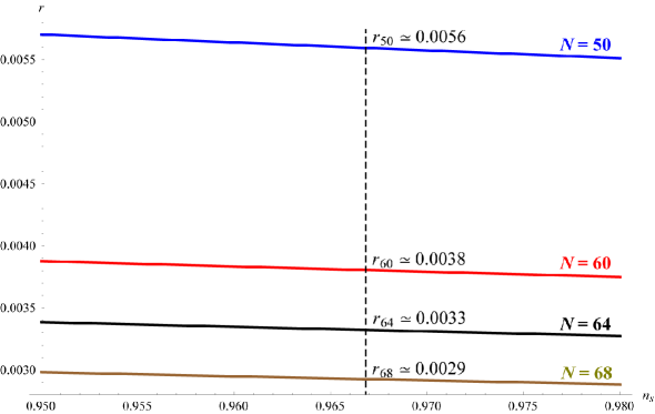
The relation (2.20) is drawn for some interesting values of N𝑁N in Fig.1. The values of rπ‘Ÿr, are well below the limit of BKP, 2015 (r<0.12π‘Ÿ0.12r<0.12).

Refer to caption
FigureΒ 1: The rβˆ’nsπ‘Ÿsubscript𝑛𝑠r-n_{s} relation in R2superscript𝑅2R^{2}-inflation for N=50,60,64𝑁506064N=50,60,64, and 68. All values of rNsubscriptπ‘Ÿπ‘{r_{N}} at ns≃0.968similar-to-or-equalssubscript𝑛𝑠0.968{n_{s}}\simeq 0.968, are well below upper limit of r(<0.12)annotatedπ‘Ÿabsent0.12r(<0.12) by BKP, 2015.

3 The electromagnetic spectra generated in R2superscript𝑅2R^{2}-inflation

One can write the electromagnetic equation, for AΞΌsubscriptπ΄πœ‡{A_{\mu}}from the Lagrangian, (1.1), as,

βˆ‚ΞΌ[βˆ’g​gμ​ν​gα​β​f2​(Ο•,t)​Fν​β]=0,subscriptπœ‡delimited-[]𝑔superscriptπ‘”πœ‡πœˆsuperscript𝑔𝛼𝛽superscript𝑓2italic-ϕ𝑑subscriptπΉπœˆπ›½0{\partial_{\mu}}\left[{\sqrt{-g}{g^{\mu\nu}}{g^{\alpha\beta}}{f^{2}}\left({\phi,t}\right){F_{\nu\beta}}}\right]=0, (3.1)

where, g𝑔g is the determinant of the flat FRW space-time metric gμ​νsubscriptπ‘”πœ‡πœˆ{g_{\mu\nu}} defined as,

d​s2=gμ​ν​d​xμ​d​xΞ½=βˆ’d​t2+a2​(t)​d​x2=gμ​ν′​d​xμ​d​xΞ½=βˆ’a2​(Ξ·)​(d​η2+d​x2).𝑑superscript𝑠2subscriptπ‘”πœ‡πœˆπ‘‘superscriptπ‘₯πœ‡π‘‘superscriptπ‘₯πœˆπ‘‘superscript𝑑2superscriptπ‘Ž2𝑑𝑑superscriptπ‘₯2subscriptsuperscriptπ‘”β€²πœ‡πœˆπ‘‘superscriptπ‘₯πœ‡π‘‘superscriptπ‘₯𝜈superscriptπ‘Ž2πœ‚π‘‘superscriptπœ‚2𝑑superscriptπ‘₯2d{s^{2}}={g_{\mu\nu}}d{x^{\mu}}\;d{x^{\nu}}=-d{t^{2}}+{a^{2}}\left(t\right)d{x^{2}}={g^{\prime}_{\mu\nu}}d{x^{\mu}}\;d{x^{\nu}}=-{a^{2}}\left(\eta\right)\left({d{\eta^{2}}+d{x^{2}}}\right). (3.2)

Hence, βˆ’g=a3​(t)𝑔superscriptπ‘Ž3𝑑\sqrt{-g}={a^{3}}\left(t\right), βˆ’gβ€²=a4​(Ξ·)superscript𝑔′superscriptπ‘Ž4πœ‚\sqrt{-g^{\prime}}={a^{4}}\left(\eta\right), and gμ​ν​gμ​β=δβνsuperscriptπ‘”πœ‡πœˆsubscriptπ‘”πœ‡π›½superscriptsubscriptπ›Ώπ›½πœˆ{g^{\mu\nu}}{g_{\mu\beta}}=\delta_{\beta}^{\nu}. Adopting the Coulomb (radiation) gauge, βˆ‚iAi​(t,x)=0subscript𝑖superscript𝐴𝑖𝑑π‘₯0{\partial_{i}}{A^{i}}\left({t,x}\right)=0, and the charge-free condition A0​(t,x)=0subscript𝐴0𝑑π‘₯0{A_{0}}\left({t,x}\right)=0, Eq.(3.1) can be written as

AΒ¨i​(t,x)+(H+2​fΛ™f)​AΛ™i​(t,x)βˆ’βˆ‚jβˆ‚jAi​(t,x)=0.subscript¨𝐴𝑖𝑑π‘₯𝐻2˙𝑓𝑓subscript˙𝐴𝑖𝑑π‘₯subscript𝑗superscript𝑗subscript𝐴𝑖𝑑π‘₯0{\ddot{A}_{i}}\left({t,x}\right)+\left({H+\frac{{2\dot{f}}}{f}}\right){\dot{A}_{i}}\left({t,x}\right)-{\rm{\;}}{\partial_{j}}{\partial^{j}}{A_{i}}\left({t,x}\right)=0. (3.3)

In conformal time, the above equation can be written as

Aβ€²β€²i​(Ξ·,x)+2​fβ€²f​Aβ€²i​(Ξ·,x)βˆ’a2​(Ξ·)β€‹βˆ‚jβˆ‚jAi​(Ξ·,x)=0.subscriptsuperscriptAβ€²β€²π‘–πœ‚π‘₯2superscript𝑓′𝑓subscriptsuperscriptAβ€²π‘–πœ‚π‘₯superscriptπ‘Ž2πœ‚subscript𝑗superscript𝑗subscriptAπ‘–πœ‚π‘₯0{{\rm{A^{\prime\prime}}}_{i}}\left({\eta,x}\right)+2\frac{{f^{\prime}}}{f}{{\rm{A^{\prime}}}_{i}}\left({\eta,x}\right)-{a^{2}}\left(\eta\right){\rm{\;}}{\partial_{j}}{\partial^{j}}{{\rm{A}}_{i}}\left({\eta,x}\right)=0. (3.4)

Define the function, AΒ―i​(Ξ·,x)=f​(Ξ·)​Ai​(Ξ·,x)subscriptΒ―Aπ‘–πœ‚π‘₯π‘“πœ‚subscriptAπ‘–πœ‚π‘₯{{\rm{\bar{A}}}_{i}}\left({\eta,x}\right)=f\left(\eta\right){{\rm{A}}_{i}}\left({\eta,x}\right), and plug it into (3.4),

Aβ€²β€²iΒ―+fβ€²β€²f​AΒ―iβˆ’a2β€‹βˆ‚jβˆ‚jAΒ―i​(Ξ·,x)=0.Β―subscriptsuperscriptA′′𝑖superscript𝑓′′𝑓subscriptΒ―A𝑖superscriptπ‘Ž2subscript𝑗superscript𝑗subscriptΒ―Aπ‘–πœ‚π‘₯0\overline{{{{\rm{A^{\prime\prime}}}}_{i}}}+\frac{{f^{\prime\prime}}}{f}{{\rm{\bar{A}}}_{i}}-\;{a^{2}}{\rm{\;}}{\partial_{j}}{\partial^{j}}{{\rm{\bar{A}}}_{i}}\left({\eta,x}\right)=0. (3.5)

On the other hand, the quantization of AΒ―isubscriptΒ―A𝑖{{\rm{\bar{A}}}_{i}} can be written in terms of creation and annihilation operators, b†λsubscriptsuperscriptπ‘β€ πœ†{b^{\dagger}}_{\lambda} and bλ​(k)subscriptπ‘πœ†π‘˜{b_{\lambda}}\left(k\right), as,

AΒ―i​(Ξ·,x)=∫d3​k(2​π)3/2β€‹βˆ‘Ξ»=12Ο΅i​λ​(k)​[bλ​(k)β€‹π’œβ€‹(Ξ·,k)​ei​k.x+b†λ​(k)β€‹π’œβˆ—β€‹(Ξ·,k)​eβˆ’i​k.x],subscriptΒ―Aπ‘–πœ‚π‘₯superscript𝑑3π‘˜superscript2πœ‹32superscriptsubscriptπœ†12subscriptitalic-Ο΅π‘–πœ†π‘˜delimited-[]subscriptπ‘πœ†π‘˜π’œπœ‚π‘˜superscript𝑒formulae-sequenceπ‘–π‘˜π‘₯subscriptsuperscriptπ‘β€ πœ†π‘˜superscriptπ’œπœ‚π‘˜superscript𝑒formulae-sequenceπ‘–π‘˜π‘₯{{\rm{\bar{A}}}_{i}}\left({\eta,x}\right)=\int{\frac{{{d^{3}}k}}{{{{\left({2\pi}\right)}^{3/2}}}}\mathop{\sum}\limits_{\lambda=1}^{2}{\epsilon_{i\lambda}}\left(k\right)[{b_{\lambda}}\left(k\right){\cal A}\left({\eta,k}\right){e^{ik.x}}+{b^{\dagger}}_{\lambda}\left(k\right){{\cal A}^{*}}\left({\eta,k}\right){e^{-ik.x}}]}, (3.6)

where, Ο΅i​λsubscriptitalic-Ο΅π‘–πœ†{\epsilon_{i\lambda}} is the transverse polarization vector, and k=2β€‹Ο€Ξ»π‘˜2πœ‹πœ†k=\frac{{2\pi}}{\lambda}, is the commoving wave number. Substituting (3.6) into (3.5),

π’œβ€²β€²β€‹(Ξ·,k)+(k2βˆ’fβ€²β€²f)β€‹π’œβ€‹(Ξ·,k)=0,superscriptπ’œβ€²β€²πœ‚π‘˜superscriptπ‘˜2superscriptπ‘“β€²β€²π‘“π’œπœ‚π‘˜0{\cal A}^{\prime\prime}\left({\eta,k}\right)+\left({{k^{2}}-\frac{{f^{\prime\prime}}}{f}}\right){\cal A}\left({\eta,k}\right)=0, (3.7)

where we have used, βˆ‚j=gj​kβ€‹βˆ‚k=(Ξ΄j​ka2)β€‹βˆ‚ksuperscript𝑗superscriptπ‘”π‘—π‘˜subscriptπ‘˜superscriptπ›Ώπ‘—π‘˜superscriptπ‘Ž2subscriptπ‘˜{\partial^{j}}={g^{jk}}{\partial_{k}}=\left({\frac{{{\delta^{jk}}}}{{{a^{2}}}}}\right){\partial_{k}}. Similarly, the stress energy tensor, Tμ​νsubscriptπ‘‡πœ‡πœˆ{T_{\mu\nu}}, can be written in terms of the action, S𝑆S, as,

Tμ​ν=βˆ’2βˆ’g​δ​Sδ​gμ​ν=(βˆ‚ΞΌΟ•)​(βˆ‚Ξ½Ο•)βˆ’f2​(Ο•,t)​gα​β​Fμ​α​FΞ²β€‹Ξ½βˆ’14​gμ​ν​gα​β​gγ​δ​f2​(Ο•,t)​Fβ​δ​Fα​γ.subscriptπ‘‡πœ‡πœˆ2𝑔𝛿𝑆𝛿superscriptπ‘”πœ‡πœˆsubscriptπœ‡italic-Ο•subscript𝜈italic-Ο•superscript𝑓2italic-ϕ𝑑superscript𝑔𝛼𝛽subscriptπΉπœ‡π›ΌsubscriptπΉπ›½πœˆ14subscriptπ‘”πœ‡πœˆsuperscript𝑔𝛼𝛽superscript𝑔𝛾𝛿superscript𝑓2italic-ϕ𝑑subscript𝐹𝛽𝛿subscript𝐹𝛼𝛾{T_{\mu\nu}}=-\frac{2}{{\sqrt{-g}}}\frac{{\delta S}}{{\delta{g^{\mu\nu}}}}=\left({{\partial_{\mu}}\phi}\right)\left({{\partial_{\nu}}\phi}\right)-{f^{2}}\left({\phi,{\rm{}}t}\right){g^{\alpha\beta}}{F_{\mu\alpha}}{F_{\beta\nu}}-\frac{1}{4}{g_{\mu\nu}}{g^{\alpha\beta}}{g^{\gamma\delta}}{f^{2}}\left({\phi,{\rm{}}t}\right){F_{\beta\delta}}{F_{\alpha\gamma}}. (3.8)

For the magnetic field, we ignore the kinetic part (first term) because it does not contribute to the electromagnetic field. Then magnetic part of Tμ​νsubscriptπ‘‡πœ‡πœˆ{T_{\mu\nu}},

T00B=14​a2​gi​j​gk​l​f2​(Ο•,t)​(βˆ‚jAlβˆ’βˆ‚lAj)​(βˆ‚iAkβˆ’βˆ‚kAi)=f2​(Ο•,t)2​a2​Bμ​BΞΌ.superscriptsubscript𝑇00𝐡14superscriptπ‘Ž2superscript𝑔𝑖𝑗superscriptπ‘”π‘˜π‘™superscript𝑓2italic-ϕ𝑑subscript𝑗subscript𝐴𝑙subscript𝑙subscript𝐴𝑗subscript𝑖subscriptπ΄π‘˜subscriptπ‘˜subscript𝐴𝑖superscript𝑓2italic-ϕ𝑑2superscriptπ‘Ž2subscriptπ΅πœ‡superscriptπ΅πœ‡T_{00}^{B}=\frac{1}{4}{a^{2}}{g^{ij}}{g^{kl}}{f^{2}}\left({\phi,{\rm{}}t}\right)({\partial_{j}}{A_{l}}-{\partial_{l}}{A_{j}})({\partial_{i}}{A_{k}}-{\partial_{k}}{A_{i}})=\frac{{{f^{2}}\left({\phi,{\rm{}}t}\right)}}{2}{a^{2}}{B_{\mu}}{B^{\mu}}. (3.9)

The energy density of the magnetic field, ρBsubscript𝜌𝐡{\rho_{B}} is found by taking the average of the component of the stress energy tensor. Finally, the spectrum of the magnetic field is given [24] by

d​ρBd​ln​k=12​π2​(ka)4​k​|π’œβ€‹(Ξ·,k)|2.𝑑subscriptπœŒπ΅π‘‘lnπ‘˜12superscriptπœ‹2superscriptπ‘˜π‘Ž4π‘˜superscriptπ’œπœ‚π‘˜2\frac{{d{\rho_{B}}}}{{d{\rm{ln}}k}}=\frac{1}{{2{\pi^{2}}}}{\left({\frac{k}{a}}\right)^{4}}k{\left|{{\cal A}\left({\eta,k}\right)}\right|^{2}}. (3.10)

Similarly, the spectrum of the electric field is given by

d​ρEd​ln​k=f22​π2​k3a4​|[π’œβ€‹(Ξ·,k)f]β€²|2.𝑑subscriptπœŒπΈπ‘‘lnπ‘˜superscript𝑓22superscriptπœ‹2superscriptπ‘˜3superscriptπ‘Ž4superscriptsuperscriptdelimited-[]π’œπœ‚π‘˜π‘“β€²2\frac{d{\rho_{E}}}{d{\rm{ln}}k}=\frac{f^{2}}{2\pi^{2}}\frac{{{k^{3}}}}{{{a^{4}}}}{\left|{{\left[\frac{{\cal A}\left({\eta,{\rm{}}k}\right)}{f}\right]}^{\prime}}\right|^{2}}. (3.11)

Therefore, to calculate the electromagnetic spectra, one has to find π’œβ€‹(Ξ·,k)π’œπœ‚π‘˜{\cal A}\left({\eta,{\rm{}}k}\right), which can be achieved by solving (3.7). But first, we need to specify the coupling function, f​(Ο•)𝑓italic-Ο•f\left(\phi\right). Assuming that the relation between the coupling function and scale factor is of the power law form [8], f​(Ξ·)∝aΞ±proportional-toπ‘“πœ‚superscriptπ‘Žπ›Όf\left(\eta\right){\rm{\;}}\propto{\rm{\;}}{a^{\alpha}}, where, α𝛼\alpha is free index to be determined later from the shape of the spectrum of PMF. Then, by combining (2.1) and (2.2) in the slow roll limit,

f​(Ο•)∝e​x​p​[βˆ’Ξ±3​MPl2β€‹βˆ«Ο•VVϕ​d​ϕ].proportional-to𝑓italic-ϕ𝑒π‘₯𝑝delimited-[]𝛼3superscriptsubscript𝑀Pl2superscriptitalic-ϕ𝑉subscript𝑉italic-ϕ𝑑italic-Ο•f\left(\phi\right){\rm{\;}}\propto exp\left[{-\frac{\alpha}{{3\;{M_{{\rm{Pl}}}}^{2}}}\mathop{\smallint}\limits^{\phi}\frac{V}{{{V_{\phi}}}}d\phi}\right]. (3.12)

Substituting (2.19) into (1.2) and (3.12) yields the coupling function as a function of N𝑁N,

f​(N)=D​[(4​N3)Ξ±4​eβˆ’N​α3],𝑓𝑁𝐷delimited-[]superscript4𝑁3𝛼4superscripte𝑁𝛼3f\left(N\right){\rm{\;}}=D\left[{{{\left({\frac{{4N}}{3}}\right)}^{\frac{\alpha}{4}}}{{\rm{e}}^{-\frac{{N\alpha}}{3}}}}\right], (3.13)

where, D𝐷D is a coupling constant. Substituting (3.13) into (3.7) gives,

π’œβ€²β€²β€‹(Ξ·,k)+(k2βˆ’Y​(Ξ·))β€‹π’œβ€‹(Ξ·,k)=0,superscriptπ’œβ€²β€²πœ‚π‘˜superscriptπ‘˜2π‘Œπœ‚π’œπœ‚π‘˜0{\cal A}^{\prime\prime}\left({\eta,k}\right)+\left({{k^{2}}-Y\left(\eta\right)}\right){\cal A}\left({\eta,k}\right)=0, (3.14)

here the function Y​(Ξ·)=fβ€²β€²fπ‘Œπœ‚superscript𝑓′′𝑓Y\left(\eta\right)=\frac{{f^{\prime\prime}}}{f}. Hence, we need to write the derivative in terms of e-folds number, N𝑁N. In the next two sections, the electromagnetic spectra are calculated for both de Sitter and power law expansion.

3.1 Inflationary electromagnetic spectra in de Sitter expansion

Shortly after the onset of inflation the value of H𝐻H becomes very high and is approximately constant, but later on, it decreases as the value of the field changes. For the zeroth approximation and after the first few e-foldings, we can consider H as a constant ratio. That is basically the de Sitter expansion, which is exactly exponential expansion as described by (2.12). In fact, de Sitter model does not have graceful exit from inflation [46]. But it can be assumed as a valid approximation on part of the inflation. Assuming, a​(Ξ·i)=constπ‘Žsubscriptπœ‚π‘–consta({\eta_{i}})={\rm{const}}, and substituting of (2.13) into (2.18) and differentiating both sides, yields that, βˆ‚Ξ·β€‹Ξ·f​(Ξ·)=Ξ·βˆ’2β€‹βˆ‚N​Nf​(N)subscriptπœ‚πœ‚π‘“πœ‚superscriptπœ‚2subscript𝑁𝑁𝑓𝑁{\partial_{\eta\eta}}f(\eta)={\eta^{-2}}{\partial_{NN}}f(N). Therefore, the function Y​(Ξ·)π‘Œπœ‚Y\left(\eta\right) can be written as,

Yd​S​(Ξ·)=α​[(3βˆ’4​N)2β€‹Ξ±βˆ’36]144​N2​η2.subscriptπ‘Œπ‘‘π‘†πœ‚π›Όdelimited-[]superscript34𝑁2𝛼36144superscript𝑁2superscriptπœ‚2{Y_{dS}}\left(\eta\right)=\frac{{\alpha\left[{{{\left({3-4N}\right)}^{2}}\alpha-36}\right]}}{{144{N^{2}}{\eta^{2}}}}. (3.15)

Also, as the variation in N𝑁N is very small comparison with the variation in Ξ·πœ‚\eta, we will assume that N𝑁N is quasi-constant and we will not write it as a function of conformal time explicitly in Eq.(36). Therefore, substituting of (3.15) into (3.14), yields,

π’œβ€‹(Ξ·,k)=(k​η)1/2​[C1​(k)​Jχ​(k​η)+C2​(k)​Jβˆ’Ο‡β€‹(k​η)],π’œπœ‚π‘˜superscriptπ‘˜πœ‚12delimited-[]subscript𝐢1π‘˜subscriptπ½πœ’π‘˜πœ‚subscript𝐢2π‘˜subscriptπ½πœ’π‘˜πœ‚{\cal A}\left({\eta,k}\right)={\left({k\eta}\right)^{1/2}}\left[{{C_{1}}\left(k\right)\;{J_{\chi}}\left({k\eta}\right)+{C_{2}}\left(k\right)\;{J_{-\chi}}\left({k\eta}\right)}\right], (3.16)

where, Jχ​(k​η)subscriptπ½πœ’π‘˜πœ‚{J_{\chi}}\left({k\eta}\right), is the Bessel function of the first kind, and the argument of the function,

Ο‡d​S​(Ξ±,N)=36​N2βˆ’36​α+(3βˆ’4​N)2​α212​N.subscriptπœ’π‘‘π‘†π›Όπ‘36superscript𝑁236𝛼superscript34𝑁2superscript𝛼212𝑁{\chi_{dS}}(\alpha,N)=\frac{{\sqrt{36{N^{2}}-36\alpha+{{\left({3-4N}\right)}^{2}}{\alpha^{2}}}}}{{12N}}. (3.17)

The relevant PMF is obtained in the long wavelength regime, kβ‰ͺ1much-less-thanπ‘˜1k\ll 1 (outside Hubble radius). In this limit, Eq.(3.16) can be written as [24],

π’œkβ‰ͺ1​(Ξ·,k)=(k)βˆ’1/2​[D1​(Ο‡)​(k​η)Ο‡+12+D2​(Ο‡)​(k​η)12βˆ’Ο‡].subscriptπ’œmuch-less-thanπ‘˜1πœ‚π‘˜superscriptπ‘˜12delimited-[]subscript𝐷1πœ’superscriptπ‘˜πœ‚πœ’12subscript𝐷2πœ’superscriptπ‘˜πœ‚12πœ’{{\cal A}_{k\ll 1}}\left({\eta,k}\right)={\left(k\right)^{-1/2}}\left[{{D_{1}}\left(\chi\right)\;{{\left({k\eta}\right)}^{\chi+\frac{1}{2}}}+{D_{2}}\left(\chi\right){{\left({k\eta}\right)}^{\frac{1}{2}-\chi}}}\right]. (3.18)

The constants, D1​(Ο‡)subscript𝐷1πœ’\;{D_{1}}\left(\chi\right) and D2​(Ο‡)subscript𝐷2πœ’{D_{2}}\left(\chi\right), can be fixed by using the normalization of π’œβ€‹(Ξ·,k)π’œπœ‚π‘˜{\cal A}\left({\eta,{\rm{}}k}\right) and the other limit,

π’œk≫1​(Ξ·,k)β†’eβˆ’k​η​/​2​kβ†’subscriptπ’œmuch-greater-thanπ‘˜1πœ‚π‘˜superscriptπ‘’π‘˜πœ‚/2π‘˜{{\cal A}_{k\gg 1}}\left({\eta,{\rm{}}k}\right)\to{{{e^{-k\eta}}}\mathord{\left/{\vphantom{{{e^{-k\eta}}}{\sqrt{2k}}}}\right.\kern-1.2pt}{\sqrt{2k}}}

. Thus, they can be written as

D1​(Ο‡)=Ο€2χ​eβˆ’i​π​(Ο‡+12)/2Γ​(Ο‡+1)​cos⁑(π​(Ο‡+12)),D2​(Ο‡)=Ο€21βˆ’Ο‡β€‹eβˆ’i​π​(Ο‡+32)/2Γ​(1βˆ’Ο‡)​cos⁑(π​(Ο‡+12)).formulae-sequencesubscript𝐷1πœ’πœ‹superscript2πœ’superscriptπ‘’π‘–πœ‹πœ’122Ξ“πœ’1πœ‹πœ’12subscript𝐷2πœ’πœ‹superscript21πœ’superscriptπ‘’π‘–πœ‹πœ’322Ξ“1πœ’πœ‹πœ’12{D_{1}}\left(\chi\right)=\frac{{\sqrt{\pi}}}{{{2^{\chi}}}}\;\frac{{{e^{-i\pi(\chi+\frac{1}{2})/2}}}}{{{\rm{\Gamma}}\left({\chi+1}\right)\cos\left({\pi(\chi+\frac{1}{2})}\right)}},{\rm{}}{D_{2}}\left(\chi\right)=\frac{{\sqrt{\pi}}}{{{2^{1-\chi}}}}\;\frac{{{e^{-i\pi\left({\chi+\frac{3}{2}}\right)/2}}}}{{{\rm{\Gamma}}\left({1-\chi}\right)\cos\left({\pi(\chi+\frac{1}{2})}\right)}}. (3.19)

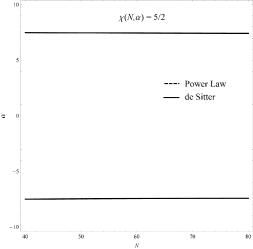
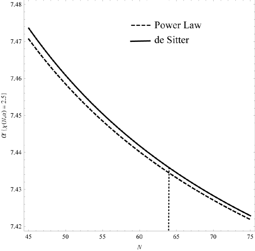
By substituting (3.18) into (3.10)-(3.11), we get the spectra of the magnetic and electric fields. If the PMF is scale invariant, then the magnetic spectrum should be constant, which could be achieved at Ο‡=5/2πœ’52\chi=5/2. This value can only be obtained around, Ξ±β‰ˆ{βˆ’7.44, 7.44}𝛼7.447.44\alpha\approx\{-7.44,\;{\rm{}}7.44\}, see Fig.2.

Refer to caption
FigureΒ 2: The Ξ±βˆ’N𝛼𝑁\alpha-N relation, at χ​(N,Ξ±)=5/2πœ’π‘π›Ό52\chi(N,\alpha)=5/2, the case at which we can generate the scale invariant PMF.

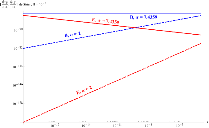
Although these values of α𝛼\alpha are too high, which may exceed dynamo limit [24], we adopt the positive value, Ξ±β‰ˆ7.44𝛼7.44\alpha\approx 7.44. In the last section, we will discuss this point. So, let us assume it is valid at this point and use it to investigate the electromagnetic spectra generated by f2​F​Fsuperscript𝑓2𝐹𝐹{f^{2}}FF for long wavelength approximation (kβ‰ͺ1much-less-thanπ‘˜1k\ll 1). From (3.10)-(3.11), one can plot the electromagnetic spectra for different values of H𝐻H and α𝛼\alpha, see Fig.3, for H=10βˆ’5​MPl𝐻superscript105subscript𝑀PlH={10^{-5}}{M_{{\rm{Pl}}}}, which is around the Planck, 2015 upper limit of pivot Hubble parameter, (Hβˆ—<3.6Γ—10βˆ’5​MPlsubscript𝐻3.6superscript105subscript𝑀Pl{H_{*}}<3.6\times{10^{-5}}{M_{{\rm{Pl}}}}) [37]. The pivot moment is the time when the commoving scale (kβˆ—=aβˆ—β€‹Hβˆ—β‰ƒ0.05​M​p​cβˆ’1subscriptπ‘˜subscriptπ‘Žsubscript𝐻similar-to-or-equals0.05𝑀𝑝superscript𝑐1{k_{*}}={a_{*}}{\rm{}}{H_{*}}\simeq 0.05Mp{c^{-1}}) exits the Hubble radius. In this case, the scale invariant PMF can be generated and the backreaction problem may be avoided at α≃7.4359similar-to-or-equals𝛼7.4359\alpha\simeq 7.4359. However, for Ξ±=2𝛼2\alpha=2, the backreaction problem can be avoided easily, but the scale invariant PMF is not generated, see Fig.3.
Refer to caption
FigureΒ 3: The EM spectra for Ξ±=[2,7.4359]𝛼27.4359\alpha=\left[2,7.4359\right], N=64𝑁64N=64, Ξ·=βˆ’10βˆ’2πœ‚superscript102\eta=-{10^{-2}} and the expansion rate , H=10βˆ’5​MPl𝐻superscript105subscript𝑀PlH={10^{-5}}{M_{{\rm{Pl}}}}. For Ξ±=2𝛼2\alpha=2, the scale invariant PMF cannot be achieved although the backreaction problem is easily to be avoided. However, for χ​(N,Ξ±)=5/2πœ’π‘π›Ό52\chi(N,\alpha)=5/2 (Ξ±=7.4359𝛼7.4359\alpha=7.4359), the scale invariant PMF can be generated and the magnetic field energy is less than the electric field which can avoid the backreaction problem.

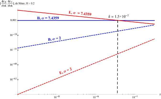
On the other hand, in the large expansion rate case, H=0.2​MPl𝐻0.2subscript𝑀PlH=0.2{M_{{\rm{Pl}}}}, the scale invariant PMF can be generated at α≃7.4359similar-to-or-equals𝛼7.4359\alpha\simeq 7.4359 but the problem of backreaction may not be avoided in the low, kβ‰ͺ1much-less-thanπ‘˜1k\ll 1, see Fig.4. In fact, this value of H𝐻H is way above the constraint upper limit [37], but we use it to decide the scale at which the electric field exceeds magnetic field (k∼1.5Γ—10βˆ’5similar-toπ‘˜1.5superscript105k\sim 1.5\times{10^{-5}}). Hence, we can use this value of the wavenumber as an upper limit in this case. Again, for Ξ±=2𝛼2\alpha=2, the backreaction problem can be avoided easily, but the scale invariant PMF is not maintained throughout the inflationary era.
Refer to caption
FigureΒ 4: The EM spectra for Ξ±=[2,7.4359]𝛼27.4359\alpha=\left[2,7.4359\right], N=64𝑁64N=64, Ξ·=βˆ’10βˆ’2πœ‚superscript102\eta=-{10^{-2}} and the expansion rate, H=0.2​MPl𝐻0.2subscript𝑀PlH=0.2{M_{{\rm{Pl}}}}. For Ξ±=2𝛼2\alpha=2, the scale invariant PMF cannot be achieved although the backreaction problem is easily to be avoided. However, for χ​(N,Ξ±)=5/2πœ’π‘π›Ό52\chi(N,\alpha)=5/2 (α≃7.4359similar-to-or-equals𝛼7.4359\alpha\simeq 7.4359), the scale invariant PMF can be generated but the magnetic field energy is less than the electric field for low wavenumber. The PMF exceeds the electric fields at, k∼1.5Γ—10βˆ’5similar-toπ‘˜1.5superscript105k\sim 1.5\times{10^{-5}}.

The value of the index, α𝛼\alpha, at which the scale invariant PMF can be generated, varies as the value of N𝑁N changes. There is a slit different between this relation in de Sitter and power law expansion, see Fig.5. These values are around, α∼7.44similar-to𝛼7.44\alpha\sim 7.44, for an interesting values of e-folds, (50<N<7050𝑁7050<N<70). The validity of α∼7.44similar-to𝛼7.44\alpha\sim 7.44 will be discussed in the section. 6, but from now onward, we adopt this value at N=64𝑁64N=64 to study the scale invariant PMF. In general, the whole results of de Sitter are very close to the power law results but both of them will be presented for a completeness.
Refer to caption
FigureΒ 5: The relation between α𝛼\alpha and N𝑁N at which χ​(N,Ξ±)=5/2πœ’π‘π›Ό52\chi(N,\alpha)=5/2, for both de Sitter and power law expansion. For the interesting range of N​(50<N<70)𝑁50𝑁70N{\rm{(50<}}N{\rm{<70)}}, the value of α𝛼\alpha is around, α∼7.44.similar-to𝛼7.44\alpha\sim{7.44.}.

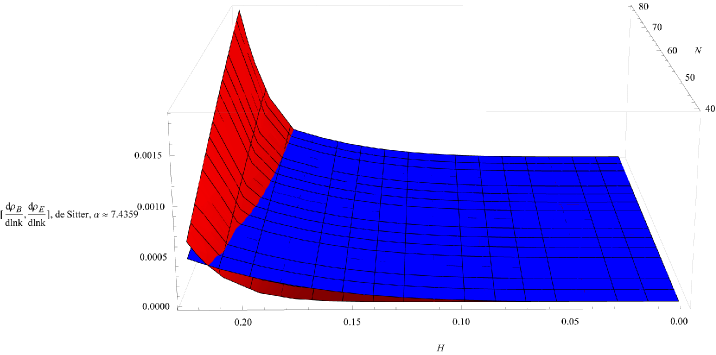
First, let us draw the relation between electromagnetic spectra, Hubble parameter, H𝐻H, and e-folding number, N𝑁N, see Fig.6. It is clear, that, for the values of H≀0.2​MPl𝐻0.2subscript𝑀PlH\leq 0.2{M_{{\rm{Pl}}}}, the backreaction problem may be avoided for all interesting values of N𝑁N. Therefore, one can consider H∼0.2​MPlsimilar-to𝐻0.2subscript𝑀PlH\sim 0.2{M_{{\rm{Pl}}}}, as an upper limit of expansion rate below which, the backreaction problem can be avoided. The current investigation will be bounded in 10βˆ’5​MPl<H<0.2​MPlsuperscript105subscript𝑀Pl𝐻0.2subscript𝑀Pl{10^{-5}}{M_{{\rm{Pl}}}}<H<0.2{M_{{\rm{Pl}}}}.

Refer to caption
FigureΒ 6: The relation between the EM spectra, Hubble parameter H𝐻H, and e-folds number, N𝑁N for de Sitter expansion. Around H∼0.2​MPlsimilar-to𝐻0.2subscript𝑀PlH\sim 0.2{M_{{\rm{Pl}}}}, electric field can exceed the magnetic field in all interesting range of N​(50<N<70)𝑁50𝑁70N{\rm{(50<}}N{\rm{<70)}}. Hence, one can consider H∼0.2​MPlsimilar-to𝐻0.2subscript𝑀PlH\sim 0.2{M_{{\rm{Pl}}}}, as an upper limit under which the backreaction problem can be avoided.

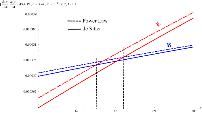
Similarly, drawing the relation between the electromagnetic spectra and e-folding number around the upper limit, H∼0.2​MPlsimilar-to𝐻0.2subscript𝑀PlH\sim 0.2{M_{{\rm{Pl}}}}, shows that below the value, N∼68similar-to𝑁68N\sim 68, the backreaction problem can be avoided, see Fig.7. Therefore, this value of N∼68similar-to𝑁68N\sim 68, can be considered as an upper limit below which, a scale invariant PMF does suffer from the backreaction problem.
Refer to caption
FigureΒ 7: The relation between the EM spectra and e-folds number, N𝑁N for both de Sitter and power law expansion around the value H∼0.2​MPlsimilar-to𝐻0.2subscript𝑀PlH\sim 0.2{M_{{\rm{Pl}}}}. The electric field can exceed the magnetic field around N∼68similar-to𝑁68N\sim 68. Hence, one can consider it as an upper limit of e-folds number before the end of inflation under which the backreaction problem can be avoided.

3.2 Inflationary electromagnetic spectra in power law expansion

For more optimal slow roll analysis that has a smooth exit from inflation, one can use the power law expansion at which the Hubble parameter is not constant but a function of field, H​(Ο•)𝐻italic-Ο•H(\phi). If the field falls below a certain value, it starts to oscillate and then converts into particles in the reheating era, right after inflation. The scale factor follows the power law, (2.10). In the slow roll limit, we can approximate . Hence, substituting (2.4) into (2.10) yields,

a​(Ξ·)=lβ€‹Ξ·βˆ’1βˆ’43​(βˆ’1+4​N3)2,π‘Žπœ‚π‘™superscriptπœ‚143superscript14𝑁32a(\eta)=l{\rm{}}{\eta^{-1-\frac{4}{{3{{\left({-1+\frac{{4N}}{3}}\right)}^{2}}}}}}, (3.20)

where, l𝑙l is the integration constant. For relatively high (Nβ‰₯50𝑁50N\geq 50), the absolute value of the exponent in (3.20) is ≲1.0003less-than-or-similar-toabsent1.0003\lesssim 1.0003, so we can approximate l≃Hβˆ’1similar-to-or-equals𝑙superscript𝐻1l\simeq{H^{-1}}. Therefore, one cannot expect significant differences between the two cases. Nevertheless, we will investigate this case to have more precise results.

Again, as we did in the last section, we will assume that N𝑁N is quasi-constant and we will not write it as a function of Ξ·πœ‚\eta explicitly. Hence in the power law expansion, we substitute (2.10) into (2.18) and differentiating both sides, yields that,

YP​L​(Ξ·)=(3βˆ’4​N)2​(63βˆ’4​N​(63+4​N​(βˆ’9+4​N)))2​α​(βˆ’36+(3βˆ’4​N)2​α)144​N2​(21+8​N​(βˆ’3+2​N))4​η2,subscriptπ‘Œπ‘ƒπΏπœ‚superscript34𝑁2superscript634𝑁634𝑁94𝑁2𝛼36superscript34𝑁2𝛼144superscript𝑁2superscript218𝑁32𝑁4superscriptπœ‚2{Y_{PL}}\left(\eta\right)=\frac{{{{\left({3-4N}\right)}^{2}}{{\left({63-4N\left({63+4N\left({-9+4N}\right)}\right)}\right)}^{2}}\alpha\left({-36+{{\left({3-4N}\right)}^{2}}\alpha}\right)}}{{144{N^{2}}{{\left({21+8N\left({-3+2N}\right)}\right)}^{4}}{\eta^{2}}}}, (3.21)
Ο‡P​L​(Ξ±,N)=(36​N2​(21+8​N​(βˆ’3+2​N))4βˆ’36​(3βˆ’4​N)2​(63βˆ’4​N​(63+4​N​(βˆ’9+4​N)))2​α+(3βˆ’4​N)4​(63βˆ’4​N​(63+4​N​(βˆ’9+4​N)))2​α2))12​N​(21+8​N​(βˆ’3+2​N))2\begin{split}{\chi_{PL}}(\alpha,N)=\frac{{\sqrt{\left(\begin{array}[]{l}36{N^{2}}{\left({21+8N\left({-3+2N}\right)}\right)^{4}}-36{\left({3-4N}\right)^{2}}{\left({63-4N\left({63+4N\left({-9+4N}\right)}\right)}\right)^{2}}\alpha\\ +{\left({3-4N}\right)^{4}}{\left({63-4N\left({63+4N\left({-9+4N}\right)}\right)}\right)^{2}}{\alpha^{2}}\end{array}\right))}}}{{12N{{\left({21+8N\left({-3+2N}\right)}\right)}^{2}}}}\end{split} (3.22)

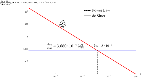
Plugging (3.21) into (3.14) yields the same solution as (3.16). In this case, Ο‡P​L​(Ξ±,N)=5/2subscriptπœ’π‘ƒπΏπ›Όπ‘52{\chi_{PL}}(\alpha,N)=5/2, at α≃{βˆ’7.4339,7.4345}similar-to-or-equals𝛼7.43397.4345\alpha\simeq\{-7.4339,{\rm{}}7.4345\}, see Fig.2 for all interesting values of N. Therefore, the scale invariant PMF can be obtained in the long wavelength regime, kβ‰ͺ1much-less-thanπ‘˜1k\ll 1 (outside Hubble radius). Also, the electromagnetic spectra can be obtained in the same way as done in last section. The results is very close to the those obtained by de Sitter case, see Fig.8-9.
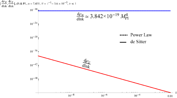
Refer to caption
FigureΒ 8: The EM spectra for Ξ±=7.4345𝛼7.4345\alpha={\rm{7}}{\rm{.4345}}, N=64𝑁64N=64, Ξ·=βˆ’10βˆ’2πœ‚superscript102\eta=-{10^{-2}} and the expansion rate, Hβ‰ˆlβˆ’1=0.2​MPl𝐻superscript𝑙10.2subscript𝑀PlH\approx{l^{-1}}=0.2{M_{{\rm{Pl}}}}. The PMF exceeds the electric fields at k∼1.5Γ—10βˆ’5similar-toπ‘˜1.5superscript105k\sim 1.5\times{10^{-5}}.
Refer to caption
FigureΒ 9: The EM spectra for Ξ±=7.4345𝛼7.4345\alpha={\rm{7}}{\rm{.4345}}, N=64𝑁64N=64, Ξ·=βˆ’10βˆ’2πœ‚superscript102\eta=-{10^{-2}} and the expansion rate at the onset of inflation, Hβ‰ˆlβˆ’1=3.6Γ—10βˆ’5​MPl𝐻superscript𝑙13.6superscript105subscript𝑀PlH\approx{l^{-1}}=3.6\times{10^{-5}}{M_{{\rm{Pl}}}}. The relation, d​ρBd​ln⁑k≫d​ρEd​ln⁑kmuch-greater-than𝑑subscriptπœŒπ΅π‘‘π‘˜π‘‘subscriptπœŒπΈπ‘‘π‘˜\frac{{d{\rho_{B}}}}{{d\ln k}}\gg\frac{{d{\rho_{E}}}}{{d\ln k}} stays valid, throughout inflation at low values of, kβ‰ͺ1much-less-thanπ‘˜1k\ll 1.

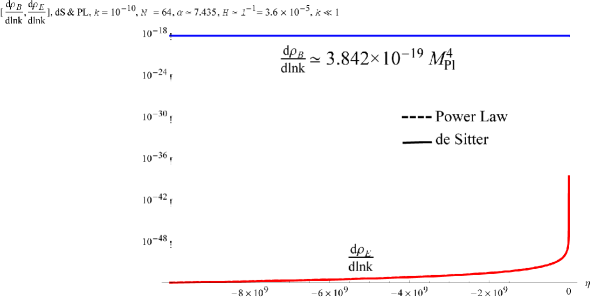
It is clear from Fig.9 that, d​ρBd​ln⁑k≫d​ρEd​ln⁑kmuch-greater-than𝑑subscriptπœŒπ΅π‘‘π‘˜π‘‘subscriptπœŒπΈπ‘‘π‘˜\frac{{d{\rho_{B}}}}{{d\ln k}}\gg\frac{{d{\rho_{E}}}}{{d\ln k}} at H≃Hβˆ—=3.6Γ—10βˆ’5​MPlsimilar-to-or-equals𝐻subscript𝐻3.6superscript105subscript𝑀PlH\simeq{H_{*}}=3.6\times{10^{-5}}{M_{{\rm{Pl}}}}. In fact that value of the Hubble parameter is the upper value during inflation or at the time of pivot scale, at which the space time exits the Hubble radius [37]. Therefore, the problem of the backreaction caused by the divergence of the electric field at kβ‰ͺ1much-less-thanπ‘˜1k\ll 1, is avoided. In order to make sure, the above relation stays valid throughout the inflationary era, we can plot the EM spectra versus the conformal time, at Ξ·β‰ͺβˆ’1much-less-thanπœ‚1\eta\ll-1, see Fig.10.

Refer to caption
FigureΒ 10: The EM spectra for Ξ±=7.4345𝛼7.4345\alpha={\rm{7}}{\rm{.4345}}, N=64𝑁64N=64, k=10βˆ’10π‘˜superscript1010k={10^{-10}} and the upper limit of Hubble parameter during inflation, Hβ‰ˆlβˆ’1=3.6Γ—10βˆ’5𝐻superscript𝑙13.6superscript105H\approx{l^{-1}}=3.6\times{10^{-5}}. The relation, d​ρBd​ln⁑k≫d​ρEd​ln⁑kmuch-greater-than𝑑subscriptπœŒπ΅π‘‘π‘˜π‘‘subscriptπœŒπΈπ‘‘π‘˜\frac{{d{\rho_{B}}}}{{d\ln k}}\gg\frac{{d{\rho_{E}}}}{{d\ln k}} stays valid, throughout the period, Ξ·β‰ͺβˆ’1much-less-thanπœ‚1\eta\ll-1 .

So far, we make sure that the electric field has negligible contribution during the inflation. However, to test the contribution of the magnetic field in the inflationary energy, one has to consider the constraints of post-inflation eras. That point will be discussed in the next section.

4 Constraining reheating parameters by PMF

It is widely believed, that there was a phase of pre-heating or reheating at the end of inflation and before the radiation dominated era [47]-[49]. In this phase, as the temperature of inflation falls to certain value, Trehsubscript𝑇reh{T_{{\rm{reh}}}}, inflaton starts oscillates around some value and decays into standard matter, that populates the Universe later. As the temperature continues to fall, the Big Bang Nucleosynthesis (BBN) starts taking place at TB​B​N∼1​M​e​Vsimilar-tosubscript𝑇𝐡𝐡𝑁1MeV{T_{BBN}}\sim 1{\rm{MeV}}. These produced particles are perturbatively decayed into radiation in the radiation era.

Initially, this process was thought it only occurs in a complicated inflationary model that has more than one field [50]-[52]. However, later on it was shown that it could be occur even in a single field model but at sub-Hubble scale of perturbations [53]-[55]. In order to constrain this phase, one has to define the reheating parameters based on both the inflationary model and the observations, like the Cosmic Microwaves Background (CMB) [56], the Large Scale Structure (LSS) [57], the BBN [58], and magnetogenesis [59].

There are two main difficulties in investigating this era. First, no direct cosmological observations can constrains the reheating parameters. Second, the physics of this period is highly uncertain. Therefore, indirect constraints of the reheating parameters are usually calculated from other cosmological observations. Also, several models have been proposed to explain this era. In this section, the effect of the scale invariant PMF on the parameters of reheating is investigated. That is basically similar to Ref [59] but by considering R2superscript𝑅2{R^{2}}-inflationary model. We adopt the new upper limits of present PMF which was constrained by Planck, 2015 [9] and the instantaneous transition to the reheating and the epochs come after. For this reason, we start by discussing the reheating parameters. Next, Next, we discuss how to constrain them by R2superscript𝑅2{R^{2}}-inflation and the present upper limit of PMF.

4.1 Reheating analysis

The reheating era can be specified mainly by three parameters, the reheating parameter, Rradsubscript𝑅rad{R_{{\rm{rad}}}}, the reheating temperature, Trehsubscript𝑇reh{T_{{\rm{reh}}}}, and the equation of state parameter, wrehsubscript𝑀reh{w_{{\rm{reh}}}} [43],[60]-[61]. The first one is defined as,

Rrad≑aendareh​(ρendρreh)1/4,subscript𝑅radsubscriptπ‘Žendsubscriptπ‘Žrehsuperscriptsubscript𝜌endsubscript𝜌reh14{R_{{\rm{rad}}}}\equiv\frac{{{a_{{\rm{end}}}}}}{{{a_{{\rm{reh}}}}}}{\left({\frac{{{\rho_{{\rm{end}}}}}}{{{\rho_{{\rm{reh}}}}}}}\right)^{1/4}}, (4.1)

where, ρ𝜌\rho is the energy density, and β€œend”and β€œreh”stand respectively to the end of inflation and the end of reheating era. From the conservation of energy during the reheating era, ρ=ρϕ+ργ𝜌subscript𝜌italic-Ο•subscriptπœŒπ›Ύ\rho={\rho_{\phi}}+{\rho_{\gamma}} and P=PΟ•+ργ/3𝑃subscript𝑃italic-Ο•subscriptπœŒπ›Ύ3P={P_{\phi}}+{\rho_{\gamma}}/3, where ρϕsubscript𝜌italic-Ο•{\rho_{\phi}} is the energy density of the scalar field of inflation and ργsubscriptπœŒπ›Ύ{\rho_{\gamma}} is the energy density of the radiation. Assuming these are the main constituent of the reheating era, one can write,

ρreh=ρend​exp⁑{βˆ’3β€‹βˆ«NendNreh[1+w​(a)]a​𝑑a}=ρend​exp⁑[βˆ’3​Δ​N​(1+wΒ―reh)],subscript𝜌rehsubscript𝜌end3superscriptsubscriptsubscript𝑁endsubscript𝑁rehdelimited-[]1π‘€π‘Žπ‘Ždifferential-dπ‘Žsubscript𝜌end3Δ𝑁1subscript¯𝑀reh{\rho_{{\rm{reh}}}}={\rho_{{\rm{end}}}}\exp\left\{{-3\int_{{N_{{\rm{end}}}}}^{{N_{{\rm{reh}}}}}{\frac{{\left[{1+w(a)}\right]}}{a}da}}\right\}={\rho_{{\rm{end}}}}\exp[-3\Delta N(1+{\bar{w}_{{\rm{reh}}}})], (4.2)

where, wΒ―rehsubscript¯𝑀reh{\bar{w}_{{\rm{reh}}}} is mean value of the equation of state parameter (P/ρ=w​(a)π‘ƒπœŒπ‘€π‘ŽP/\rho=w(a)) defined by,

wΒ―reh≑1Nrehβˆ’Nendβ€‹βˆ«NendNrehw​(a)a​𝑑a.subscript¯𝑀reh1subscript𝑁rehsubscript𝑁endsuperscriptsubscriptsubscript𝑁endsubscript𝑁rehπ‘€π‘Žπ‘Ždifferential-dπ‘Ž{\bar{w}_{{\rm{reh}}}}\equiv\frac{1}{{{N_{{\rm{reh}}}}-{N_{{\rm{end}}}}}}\int_{{N_{{\rm{end}}}}}^{{N_{{\rm{reh}}}}}{\frac{{w(a)}}{a}da}. (4.3)

Taking the logarithm of (4.1) and making use of (4.2)yields,

ln⁑Rrad=(Nrehβˆ’Nend)4​(βˆ’1+3​wΒ―reh)=1βˆ’3​wΒ―reh12​(1+wΒ―reh)​ln⁑(ρrehρend),subscript𝑅radsubscript𝑁rehsubscript𝑁end413subscript¯𝑀reh13subscript¯𝑀reh121subscript¯𝑀rehsubscript𝜌rehsubscript𝜌end\ln{R_{{\rm{rad}}}}=\frac{{\left({{N_{{\rm{reh}}}}-{N_{{\rm{end}}}}}\right)}}{4}\left({-1+3{{\bar{w}}_{{\rm{reh}}}}}\right)=\frac{{1-3{{\bar{w}}_{{\rm{reh}}}}}}{{12(1+{{\bar{w}}_{{\rm{reh}}}})}}\ln\left({\frac{{{\rho_{{\rm{reh}}}}}}{{{\rho_{{\rm{end}}}}}}}\right), (4.4)

In terms of the pivot quantities [30],

ln⁑Rrad=Nβˆ—+ln⁑(k/a0ργ1/4)+14​ln⁑(3​VendΟ΅1​Vβ£βˆ—β€‹Vβˆ—β€‹3βˆ’Ο΅1​Vβ£βˆ—3βˆ’Ο΅1​V​end)βˆ’14​ln⁑(Hβˆ—2MPl2​ϡ1​Vβ£βˆ—),subscript𝑅radsubscriptπ‘π‘˜subscriptπ‘Ž0superscriptsubscriptπœŒπ›Ύ14143subscript𝑉endsubscriptitalic-Ο΅1𝑉subscript𝑉3subscriptitalic-Ο΅1𝑉3subscriptitalic-Ο΅1𝑉end14superscriptsubscript𝐻2superscriptsubscript𝑀Pl2subscriptitalic-Ο΅1𝑉\ln{R_{{\rm{rad}}}}={N_{*}}+\ln\left({\frac{{k/{a_{0}}}}{{\rho_{\gamma}^{1/4}}}}\right)+\frac{1}{4}\ln\left({\frac{{3{V_{{\rm{end}}}}}}{{{\epsilon_{1V*}}{V_{*}}}}\frac{{3-{\epsilon_{1V*}}}}{{3-{\epsilon_{1V{\rm{end}}}}}}}\right)-\frac{1}{4}\ln\left({\frac{{H_{*}^{2}}}{{M_{{\rm{Pl}}}^{2}{\epsilon_{1V*}}}}}\right), (4.5)

On the other hand, the relation between the reheating temperature and energy density can be written as,

ρreh=Ο€230​greh​Treh4,subscript𝜌rehsuperscriptπœ‹230subscript𝑔rehsuperscriptsubscript𝑇reh4{\rho_{{\rm{reh}}}}=\frac{{{\pi^{2}}}}{{30}}{g_{{\rm{reh}}}}T_{{\rm{reh}}}^{4}, (4.6)

where, grehsubscript𝑔reh{g_{{\rm{reh}}}} is the number of relativistic degree of freedom at the end of reheating. One also can relate the reheating temperature to today temperature of CMB, T0subscript𝑇0{T_{\rm{0}}}, [62] as

Treh=T0​(a0areh)​(4311​greh)1/3=T0​(a0aeq)​eNeq​(4311​greh)1/3.subscript𝑇rehsubscript𝑇0subscriptπ‘Ž0subscriptπ‘Žrehsuperscript4311subscript𝑔reh13subscript𝑇0subscriptπ‘Ž0subscriptπ‘Žeqsuperscript𝑒subscript𝑁eqsuperscript4311subscript𝑔reh13{T_{{\rm{reh}}}}={T_{0}}\left({\frac{{{a_{0}}}}{{{a_{{\rm{reh}}}}}}}\right){\left({\frac{{43}}{{11{g_{{\rm{reh}}}}}}}\right)^{1/3}}={T_{0}}\left({\frac{{{a_{0}}}}{{{a_{{\rm{eq}}}}}}}\right){e^{{N_{{\rm{eq}}}}}}{\left({\frac{{43}}{{11{g_{{\rm{reh}}}}}}}\right)^{1/3}}. (4.7)

where, aeq/areh=eNeqsubscriptπ‘Žeqsubscriptπ‘Žrehsuperscript𝑒subscript𝑁eq{a_{{\rm{eq}}}}/{a_{{\rm{reh}}}}={e^{{N_{{\rm{eq}}}}}}, during radiation era, and β€œeq”stands for the period of equality between radiation and matter dominant phases.

In terms of the pivot scale, k=ak​Hkπ‘˜subscriptπ‘Žπ‘˜subscriptπ»π‘˜k={a_{k}}{H_{k}}, at which the commoving scale crosses the Hubble radius (horizon size) during the inflation, one can write down the relation between the scale factors and Hubble parameters [43] for different epochs of the Universe as

ka0​H0=ak​Hka0​H0=akaend​aendareh​arehaeq​aeqa0​HkH0.π‘˜subscriptπ‘Ž0subscript𝐻0subscriptπ‘Žπ‘˜subscriptπ»π‘˜subscriptπ‘Ž0subscript𝐻0subscriptπ‘Žπ‘˜subscriptπ‘Žendsubscriptπ‘Žendsubscriptπ‘Žrehsubscriptπ‘Žrehsubscriptπ‘Žeqsubscriptπ‘Žeqsubscriptπ‘Ž0subscriptπ»π‘˜subscript𝐻0\frac{k}{{{a_{0}}{H_{0}}}}=\frac{{{a_{k}}{H_{k}}}}{{{a_{0}}{H_{0}}}}=\frac{{{a_{k}}}}{{{a_{{\rm{end}}}}}}\frac{{{a_{{\rm{end}}}}}}{{{a_{{\rm{reh}}}}}}\frac{{{a_{{\rm{reh}}}}}}{{{a_{{\rm{eq}}}}}}\frac{{{a_{{\rm{eq}}}}}}{{{a_{0}}}}\frac{{{H_{k}}}}{{{H_{0}}}}. (4.8)

From (4.8), one can write the ration,

a0aeq=a0​Hkk​eβˆ’Nk​eβˆ’Nreh​eβˆ’Neq.subscriptπ‘Ž0subscriptπ‘Žeqsubscriptπ‘Ž0subscriptπ»π‘˜π‘˜superscript𝑒subscriptπ‘π‘˜superscript𝑒subscript𝑁rehsuperscript𝑒subscript𝑁eq\frac{{{a_{0}}}}{{{a_{{\rm{eq}}}}}}=\frac{{{a_{\rm{0}}}{H_{k}}}}{k}{e^{-{N_{k}}}}{e^{-{N_{{\rm{reh}}}}}}{e^{-{N_{{\rm{eq}}}}}}. (4.9)

In (4.7) and (4.9), we assume a form of exponential expansion takes place during reheating and radiation epoch too. Substituting of (4.9) into (4.7) gives,

Treh=(T0​a0k)​(4311​greh)1/3​Hk​eβˆ’Nk​eβˆ’Nreh.subscript𝑇rehsubscript𝑇0subscriptπ‘Ž0π‘˜superscript4311subscript𝑔reh13subscriptπ»π‘˜superscript𝑒subscriptπ‘π‘˜superscript𝑒subscript𝑁reh{T_{{\rm{reh}}}}=\left({\frac{{{T_{0}}{a_{0}}}}{k}}\right){\left({\frac{{43}}{{11{g_{{\rm{reh}}}}}}}\right)^{1/3}}{H_{k}}{e^{-{N_{k}}}}{e^{-{N_{{\rm{reh}}}}}}. (4.10)

If the equation of state is assumed to be constant during reheating then, ρ∝aβˆ’3​(1+w)proportional-to𝜌superscriptπ‘Ž31𝑀\rho\propto{a^{-3(1+w)}}. Also, the relation between the energy density and the potential [63] can be written as,

ρ=(1+13/Ο΅1​Vβˆ’1)​V​(Ο•).𝜌113subscriptitalic-Ο΅1𝑉1𝑉italic-Ο•\rho=\left({1+\frac{1}{{3/{\epsilon_{1V}}-1}}}\right)V\left(\phi\right). (4.11)

Making use of these relations and substituting of (4.10) into (4.6) and taking natural logarithm yields the equations of reheating e-folds numbers and temperature,

Nreh=41βˆ’3​wreh​[βˆ’Nkβˆ’ln⁑(ka0​T0)βˆ’14​ln⁑(30greh​π2)βˆ’13​ln⁑(11​greh43)βˆ’14​ln⁑(Vend)βˆ’14​ln⁑(1+13/Ο΅1​Vβˆ’1)+12​ln⁑(Ο€2​r​As2)],subscript𝑁reh413subscript𝑀rehdelimited-[]subscriptπ‘π‘˜π‘˜subscriptπ‘Ž0subscript𝑇01430subscript𝑔rehsuperscriptπœ‹21311subscript𝑔reh4314subscript𝑉end14113subscriptitalic-Ο΅1𝑉112superscriptπœ‹2π‘Ÿsubscript𝐴𝑠2\begin{split}{N_{{\rm{reh}}}}=\frac{4}{{1-3{w_{{\rm{reh}}}}}}\left[\begin{array}[]{l}-{N_{k}}-\ln\left({\frac{k}{{{a_{0}}{T_{0}}}}}\right)-\frac{1}{4}\ln\left({\frac{{30}}{{{g_{{\rm{reh}}}}{\pi^{2}}}}}\right)-\frac{1}{3}\ln\left({\frac{{11{g_{{\rm{reh}}}}}}{{43}}}\right)\\ -\frac{1}{4}\ln({V_{{\rm{end}}}})-\frac{1}{4}\ln\left({1+\frac{1}{{3/{\epsilon_{1V}}-1}}}\right)+\frac{1}{2}\ln\left({\frac{{{\pi^{2}}r{A_{s}}}}{2}}\right)\end{array}\right],\end{split} (4.12)
Treh=[(T0​a0k)​(4311​greh)1/3​Hk​eβˆ’Nk​[(1+13/Ο΅1​Vβˆ’1)​VendΟ€2​greh]βˆ’13​(1+wreh)]3​(1+wreh)3​wrehβˆ’1,subscript𝑇rehsuperscriptdelimited-[]subscript𝑇0subscriptπ‘Ž0π‘˜superscript4311subscript𝑔reh13subscriptπ»π‘˜superscript𝑒subscriptπ‘π‘˜superscriptdelimited-[]113subscriptitalic-Ο΅1𝑉1subscript𝑉endsuperscriptπœ‹2subscript𝑔reh131subscript𝑀reh31subscript𝑀reh3subscript𝑀reh1{T_{{\rm{reh}}}}={\left[{\left({\frac{{{T_{0}}{a_{0}}}}{k}}\right){{\left({\frac{{43}}{{11{g_{{\rm{reh}}}}}}}\right)}^{1/3}}{H_{k}}{e^{-{N_{k}}}}{{\left[{\left({1+\frac{1}{{3/{\epsilon_{1V}}-1}}}\right)\frac{{{V_{{\rm{end}}}}}}{{{\pi^{2}}{g_{{\rm{reh}}}}}}}\right]}^{-\frac{1}{{3(1+{w_{{\rm{reh}}}})}}}}}\right]^{\frac{{3(1+{w_{{\rm{reh}}}})}}{{3{w_{{\rm{reh}}}}-1}}}}, (4.13)

where, Vendsubscript𝑉end{V_{{\rm{end}}}} is the potential at the end of inflation and Assubscript𝐴𝑠{A_{s}} is the scalar power spectrum magnitude, obtained by (2.14). Hence, from (1.2) and the condition, Ο΅n​Vβ‰ˆ1subscriptitalic-ϡ𝑛𝑉1{\epsilon_{nV}}\approx 1, at the end of inflation, one can decide Vendsubscript𝑉end{V_{{\rm{end}}}}. In fact, the field Ο•endsubscriptitalic-Ο•end{\phi_{{\rm{end}}}} has three different values, based on which slow roll parameter is equal to unity. They are respectively, Ο•end≃0.94​MPl,1.83​MPl,1.51​MPlsimilar-to-or-equalssubscriptitalic-Ο•end0.94subscript𝑀Pl1.83subscript𝑀Pl1.51subscript𝑀Pl{\phi_{{\rm{end}}}}\simeq{\rm{0}}{\rm{.94}}{M_{{\rm{Pl}}}},{\rm{1}}{\rm{.83}}{M_{{\rm{Pl}}}},{\rm{1}}{\rm{.51}}{M_{{\rm{Pl}}}} for Ο΅1​V,Ο΅2​Vsubscriptitalic-Ο΅1𝑉subscriptitalic-Ο΅2𝑉{\epsilon_{1V}},{\rm{}}{\epsilon_{2V}} and Ο΅3​Vsubscriptitalic-Ο΅3𝑉{\epsilon_{3V}}. Therefore, we will pick the first value to avoid violating the slow roll condition.

By adopting Planck, 2015 results [37], [62]-[63], we have ka0=0.05​Mpcβˆ’1π‘˜subscriptπ‘Ž00.05superscriptMpc1\frac{k}{{{a_{0}}}}=0.05{\rm{Mp}}{{\rm{c}}^{-1}}, ns=0.9682Β±0.0062subscript𝑛𝑠plus-or-minus0.96820.0062{n_{s}}={\rm{0}}{\rm{.9682}}\pm 0.0062, As=2.196Γ—10βˆ’9subscript𝐴𝑠2.196superscript109{A_{s}}={\rm{2}}{\rm{.196}}\times{\rm{1}}{{\rm{0}}^{-9}}, and Hk<3.6Γ—10βˆ’5​MPlsubscriptπ»π‘˜3.6superscript105subscript𝑀Pl{H_{k}}<3.6\times{10^{-5}}{M_{{\rm{Pl}}}}, also by using grehβ‰ˆ100subscript𝑔reh100{g_{{\rm{reh}}}}\approx 100, Eqs.(4.12)-(4.13) become

Nreh=41βˆ’3​wreh​[61.1βˆ’Nkβˆ’ln⁑(Vend1/4Hk)],subscript𝑁reh413subscript𝑀rehdelimited-[]61.1subscriptπ‘π‘˜superscriptsubscript𝑉end14subscriptπ»π‘˜{N_{{\rm{reh}}}}=\frac{4}{{1-3{w_{{\rm{reh}}}}}}\left[{61.1-{N_{k}}-\ln\left({\frac{{V_{{\rm{end}}}^{1/4}}}{{{H_{k}}}}}\right)}\right], (4.14)
Treh=exp⁑[βˆ’34​(1+wreh)​Nreh]​[(310​π2)​(1+13/Ο΅1​Vβˆ’1)​Vend]1/4.subscript𝑇reh341subscript𝑀rehsubscript𝑁rehsuperscriptdelimited-[]310superscriptπœ‹2113subscriptitalic-Ο΅1𝑉1subscript𝑉end14{T_{{\rm{reh}}}}=\exp\left[{-\frac{3}{4}(1+{w_{{\rm{reh}}}}){N_{{\rm{reh}}}}}\right]{\left[{\left({\frac{3}{{10{\pi^{2}}}}}\right)\left({1+\frac{1}{{3/{\epsilon_{1V}}-1}}}\right){V_{{\rm{end}}}}}\right]^{1/4}}. (4.15)

The equation of state parameter at reheating era, wrehsubscript𝑀reh{w_{{\rm{reh}}}}, for general inflationary potential is usually taken in the interval, βˆ’1/3<wreh<113subscript𝑀reh1-1/3<{w_{{\rm{reh}}}}<1 [13]. But for Starobinsky inflation (R2superscript𝑅2{R^{2}}-inflation), the interval that fits well with Planck, 2015 results is 0<wreh<1/30subscript𝑀reh130<{w_{{\rm{reh}}}}<1/3 [62].

4.2 Constraining reheating parameters by the present PMF in R2superscript𝑅2{R^{2}}-inflation

The next step is to relate the reheating parameters to the present PMF which is constrained by the results of Planck, 2015 [9]. As the conformal invariance of electromagnetic field is restored after inflation, the present super Hubble magnetic field B0subscript𝐡0{B_{0}} is redshifted since the end of inflation [59] as,

B0=Bend(1+zend)2,subscript𝐡0subscript𝐡endsuperscript1subscript𝑧end2{B_{0}}=\frac{{{B_{{\rm{end}}}}}}{{{{(1+{z_{{\rm{end}}}})}^{2}}}}, (4.16)

where, Bendsubscript𝐡end{B_{{\rm{end}}}} is the magnetic field at the end of inflation and zendsubscript𝑧end{z_{{\rm{end}}}} is the redshift at the end of inflation. Hence, at the end of inflation we can write,

1+zend=a0aend=a0aeq​aeqareh​arehaend=1Rrad​(ρendργ)1/4,1subscript𝑧endsubscriptπ‘Ž0subscriptπ‘Žendsubscriptπ‘Ž0subscriptπ‘Žeqsubscriptπ‘Žeqsubscriptπ‘Žrehsubscriptπ‘Žrehsubscriptπ‘Žend1subscript𝑅radsuperscriptsubscript𝜌endsubscriptπœŒπ›Ύ141+{z_{{\rm{end}}}}=\frac{{{a_{0}}}}{{{a_{{\rm{end}}}}}}=\frac{{{a_{0}}}}{{{a_{{\rm{eq}}}}}}\frac{{{a_{{\rm{eq}}}}}}{{{a_{{\rm{reh}}}}}}\frac{{{a_{{\rm{reh}}}}}}{{{a_{{\rm{end}}}}}}=\frac{1}{{{R_{{\rm{rad}}}}}}{\left({\frac{{{\rho_{{\rm{end}}}}}}{{{\rho_{\gamma}}}}}\right)^{1/4}}, (4.17)

where,ργ∼(5.7Γ—10βˆ’125​MP​l4)similar-tosubscriptπœŒπ›Ύ5.7superscript10125superscriptsubscript𝑀𝑃𝑙4{\rho_{\gamma}}\sim(5.7\times{10^{-125}}M_{Pl}^{4}) is energy density of radiation today.

We substitute (4.17) into (4.16) and make sure there is no backreaction problem at the end of inflation, ρBend<ρendsubscript𝜌subscript𝐡endsubscript𝜌end{\rho_{{B_{{\rm{end}}}}}}<{\rho_{{\rm{end}}}}. Since, ρB=B2/2subscript𝜌𝐡superscript𝐡22{\rho_{B}}={B^{2}}/2, then combining (4.16) and (4.17) yields the constraint in reheating parameters from the present PMF [59],

Rrad≫B01/2(2​ργ)1/4.much-greater-thansubscript𝑅radsuperscriptsubscript𝐡012superscript2subscriptπœŒπ›Ύ14{R_{{\rm{rad}}}}\gg\frac{{B_{0}^{1/2}}}{{{{(2{\rho_{\gamma}})}^{1/4}}}}. (4.18)

The upper limit of present PMF calculated by Planck, 2015 is ∼10βˆ’9​Gsimilar-toabsentsuperscript109G\sim 10^{-9}\rm{G}. Therefore, the lower limit of reheating parameter is, Rrad>1.761Γ—10βˆ’2subscript𝑅rad1.761superscript102R_{\rm{rad}}>1.761\times 10^{-2}. But this limit is independent of the inflationary model. Hence, for a more accurate limit of Rradsubscript𝑅radR_{\rm{rad}} associated with R2superscript𝑅2R^{2}- inflation, one can use the result of [49] and adopting the Planck, 2015 results, at which the middle value, Nβˆ—β‰ƒ58.5similar-to-or-equalssubscriptπ‘βˆ—58.5{N_{\ast}}\simeq 58.5, if wrehsubscript𝑀rehw_{\rm{reh}} is not constant [37]. It implies that, Rrad>6.888subscript𝑅rad6.888R_{\rm{rad}}>6.888, which is three orders of magnitude more than the previous one. Therefore, the reheating in this case is more constraint by the inflationary model bound.

In order to constrain the reheating energy scale, one can substitute (4.18) into (4.4) to obtain,

ρreh>ρend​[B0(2​ργ)1/2]6​(1+wΒ―reh)1βˆ’3​wΒ―reh.subscript𝜌rehsubscript𝜌endsuperscriptdelimited-[]subscript𝐡0superscript2subscriptπœŒπ›Ύ1261subscript¯𝑀reh13subscript¯𝑀reh{\rho_{{\rm{reh}}}}>{\rho_{{\rm{end}}}}{\left[{\frac{{{B_{0}}}}{{{{(2{\rho_{\gamma}})}^{1/2}}}}}\right]^{\frac{{6(1+{{\bar{w}}_{{\rm{reh}}}})}}{{1-3{{\bar{w}}_{{\rm{reh}}}}}}}}. (4.19)

Therefore, one has to find ρendsubscript𝜌end\rho_{\rm{end}} for the model of inflation. Also, the lower limit of reheating energy density should be greater than BBN energy, ρreh>ρnucsubscript𝜌rehsubscript𝜌nuc\rho_{\rm{reh}}>\rho_{\rm{nuc}}, where ρnucsubscript𝜌nuc\rho_{\rm{nuc}} is in the order of (∼10​M​e​Vsimilar-toabsent10MeV\sim 10{\rm{MeV}}).

We can use the upper bound of the energy density of inflation derived from WMAP7, (ρend)CMB<2.789Γ—10βˆ’10​MPl4subscriptsubscript𝜌endCMB2.789superscript1010superscriptsubscript𝑀Pl4{\left({{\rho_{{\rm{end}}}}}\right)_{{\rm{CMB}}}}<2.789\times{10^{-10}}M_{{\rm{Pl}}}^{4} [56] and the lower limit of Rrad(>6.888)annotatedsubscript𝑅radabsent6.888{R_{{\rm{rad}}}}(>6.888) and substitute them into (4.17), one can find the upper bound of, 1+zend<6.828Γ—10271subscript𝑧end6.828superscript10271+{z_{{\rm{end}}}}<6.828\times{10^{27}}. If we substitute the redshift into 4.16, we can find the upper limit of magnetic field at the end of inflation, Bend<4.662Γ—1046​G​(2.3541Γ—10βˆ’5​MPl2)subscript𝐡end4.662superscript1046G2.3541superscript105superscriptsubscript𝑀Pl2{B_{{\rm{end}}}}<4.662\times{10^{46}}{\rm{G}}{\rm{(2}}.3541\times{10^{-5}}M_{{\rm{Pl}}}^{2}), where we have used, 1​Gβ‰ˆ3.3Γ—10βˆ’57​MPl21G3.3superscript1057superscriptsubscript𝑀Pl21{\rm{G}}\approx{\rm{3}}{\rm{.3}}\times{\rm{1}}{{\rm{0}}^{-57}}M_{{\rm{Pl}}}^{2}. Hence, the energy density of the magnetic field is (ρBend)CMB<1.184Γ—10βˆ’20​MPl4subscriptsubscript𝜌subscript𝐡endCMB1.184superscript1020superscriptsubscript𝑀Pl4{\left({{\rho_{{B_{{\rm{end}}}}}}}\right)_{{\rm{CMB}}}}<1.184\times{10^{-20}}M_{{\rm{Pl}}}^{4}. It is ten orders of magnitude more than the upper limit of ρendsubscript𝜌end{\rho_{{\rm{end}}}} found from CMB [56]. Therefore, the backreaction problem can be avoided easily.

On the other hand, we can use Eq.(4.11) to find the energy density at the end of inflation (Ο΅1​Vβ‰ˆ1,ρend=32​Vend)formulae-sequencesubscriptitalic-Ο΅1𝑉1subscript𝜌end32subscript𝑉end(\epsilon_{1V}\approx 1,\rho_{\rm{end}}=\frac{3}{2}V_{\rm{end}}). By adopting the value of Ξ›(∼4.0Γ—10βˆ’5​MPl)annotatedΞ›similar-toabsent4.0superscript105subscript𝑀Pl\Lambda(\sim 4.0\times 10^{-5}M_{\rm{Pl}}), calculated from the amplitude of the CMB anisotropies [30], we find (ρend)R2βˆ’inflation≃1.1Γ—10βˆ’18​MPl4similar-to-or-equalssubscriptsubscript𝜌endsuperscriptR2inflation1.1superscript1018superscriptsubscript𝑀Pl4\left(\rho_{\rm{end}}\right)_{{\rm{R}}^{2}-\rm{inflation}}\simeq 1.1\times 10^{-18}M_{\rm{Pl}}^{4}. Similarly, substituting of this value with the limit, Rrad(>6.888)annotatedsubscript𝑅radabsent6.888R_{\rm{rad}}(>6.888) into (4.16)-(4.17) implies that, 1+zend<5.414Γ—10251subscript𝑧end5.414superscript10251+z_{\rm{end}}<5.414\times{10^{25}} and (ρBend)R2βˆ’inflation<4.6788Γ—10βˆ’29​MPl4subscriptsubscript𝜌subscript𝐡endsuperscriptR2inflation4.6788superscript1029superscriptsubscript𝑀Pl4\left(\rho_{B_{\rm{end}}}\right)_{{{\rm{R}}^{2}}-\rm{inflation}}<4.6788\times 10^{-29}M_{\rm{Pl}}^{4}, which is free more from backreaction problem. Therefore, (ρBend)R2βˆ’inflationsubscriptsubscript𝜌subscript𝐡endsuperscriptR2inflation\left(\rho_{B_{\rm{end}}}\right)_{{\rm{R}}^{2}-\rm{inflation}} calculated by inflationary model and the present limits of PMF found by Planck, 2015 puts more constraints on the ρBendsubscript𝜌subscript𝐡end\rho_{B_{\rm{end}}} than the constraints found by (ρBend)CMBsubscriptsubscript𝜌subscript𝐡endCMB\left(\rho_{B_{{\rm{end}}}}\right)_{\rm{CMB}} with present limits of PMF.

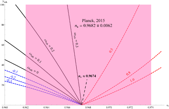
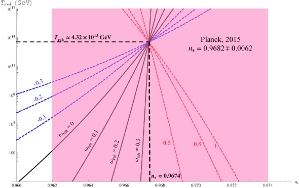
Similarly, one can plot both Nrehsubscript𝑁reh{N_{{\rm{reh}}}} and Trehsubscript𝑇reh{T_{{\rm{reh}}}} as a function of nssubscript𝑛s{n_{\rm{s}}} by using Eq.(4.15), see Fig.11-12. As we can see from Fig.12, all curves of possible wrehsubscript𝑀reh{w_{{\rm{reh}}}} intersect at Trehβ‰ˆ4.32Γ—1013​GeVsubscript𝑇reh4.32superscript1013GeV{T_{{\rm{reh}}}}\approx 4.32\times{10^{13}}{\rm{GeV}} and nsβ‰ˆ0.9674subscript𝑛s0.9674{n_{\rm{s}}}\approx 0.9674, the value of spectral index fits well with the range of Planck, 2015 for R2superscript𝑅2{R^{2}}-inflation. This temperature is much more than the range of reheating temperature obtained from CMB in the context of LFI, see Eq.(4.11) of Ref.[56]. As we use the upper limit of Hβˆ—subscript𝐻{H_{*}} in Eq.(4.14), we can consider the above value as the upper limit of Trehsubscript𝑇reh{T_{{\rm{reh}}}}.

Refer to caption
FigureΒ 11: The plot of reheating e-folds, Nrehsubscript𝑁reh{N_{{\rm{reh}}}}, versus spectral index, nssubscript𝑛s{n_{\rm{s}}}, at the end of R2superscript𝑅2{R^{2}}-inflation, for some values in βˆ’0.3<wreh<10.3subscript𝑀reh1-0.3<{w_{{\rm{reh}}}}<1. They all intersect at nsβ‰ˆ0.9674subscript𝑛s0.9674{n_{\rm{s}}}\approx 0.9674, which lies well in the Planck, 2015 range, ns=0.9682Β±0.0062subscript𝑛𝑠plus-or-minus0.96820.0062{n_{s}}={\rm{0}}{\rm{.9682}}\pm 0.0062
Refer to caption
FigureΒ 12: The plot of reheating temperature, Trehsubscript𝑇reh{T_{{\rm{reh}}}}, versus spectral index, nssubscript𝑛s{n_{\rm{s}}}, at the end of R2superscript𝑅2{R^{2}}-inflation, for some values in βˆ’0.3<wreh<10.3subscript𝑀reh1-0.3<{w_{{\rm{reh}}}}<1. They all intersect into Treh∼4.32Γ—1013​GeVsimilar-tosubscript𝑇reh4.32superscript1013GeV{T_{{\rm{reh}}}}\sim 4.32\times{10^{13}}{\rm{GeV}} at nsβ‰ˆ0.9674subscript𝑛s0.9674{n_{\rm{s}}}\approx 0.9674. The value of the temperature is below (ρend)1/4superscriptsubscript𝜌end14{({\rho_{{\rm{end}}}})^{1/4}} and the spectral index lie in the Planck, 2015 range, ns=0.9682Β±0.0062subscript𝑛𝑠plus-or-minus0.96820.0062{n_{s}}={\rm{0}}{\rm{.9682}}\pm 0.0062.

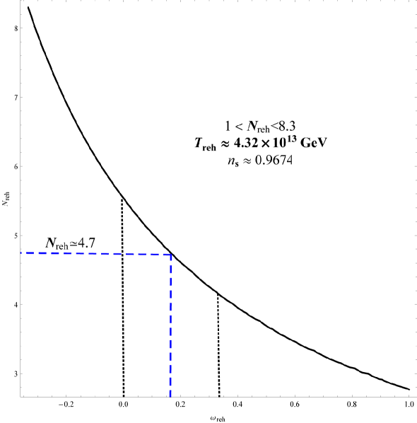
Thus, adopting the this temperature for all wrehsubscript𝑀reh{w_{{\rm{reh}}}} models of reheating, enables us to constrain the Nrehsubscript𝑁reh{N_{{\rm{reh}}}} on the range 1<Nreh<8.31subscript𝑁reh8.31<{N_{{\rm{reh}}}}<8.3, for all possible values of ,wrehsubscript𝑀reh{w_{{\rm{reh}}}} see Fig.13. The average value of Nrehsubscript𝑁reh{N_{{\rm{reh}}}} is relatively low, Nreh≃4.7similar-to-or-equalssubscript𝑁reh4.7{N_{{\rm{reh}}}}\simeq 4.7. Also, from, (4.6) one can find, ρrehβ‰ˆ3.259Γ—10βˆ’18​MPl4subscript𝜌reh3.259superscript1018superscriptsubscript𝑀Pl4{\rho_{{\rm{reh}}}}\approx 3.259\times{10^{-18}}M_{{\rm{Pl}}}^{4}, which is in the same order of magnitude of the upper limit of (ρend)R2βˆ’inflationsubscriptsubscript𝜌endsuperscriptR2inflation{\left({{\rho_{{\rm{end}}}}}\right)_{{{\rm{R}}^{2}}-{\rm{inflation}}}} and two orders of magnitude less than the upper limit of (ρBend)CMBsubscriptsubscript𝜌subscript𝐡endCMB{\left({{\rho_{{B_{{\rm{end}}}}}}}\right)_{{\rm{CMB}}}}. Interestingly enough this value of ρreh1/4​(1.035Γ—1014​GeV)superscriptsubscript𝜌reh141.035superscript1014GeV\rho_{{\rm{reh}}}^{1/4}(1.035\times{10^{14}}{\rm{GeV}}) is one order of magnitude less than the range of ρendsubscript𝜌end{\rho_{{\rm{end}}}}, obtained from CMB for the large field inflation [56], see Eq.(4.1) of the same reference. Therefore, the instantaneous reheating at which, ρendβ‰ˆΟrehsubscript𝜌endsubscript𝜌reh{\rho_{{\rm{end}}}}\approx{\rho_{{\rm{reh}}}}, can be manifested by this result.

Refer to caption
FigureΒ 13: The number of e-folds, Nrehsubscript𝑁reh{N_{{\rm{reh}}}}, during reheating, for all possible values of the equation of state parameter, βˆ’1/3<wreh<113subscript𝑀reh1-1/3<{w_{{\rm{reh}}}}<1, at nsβ‰ˆ0.9637subscript𝑛s0.9637{n_{\rm{s}}}\approx 0.9637. The range of e-folds is, 1<Nreh<8.31subscript𝑁reh8.31<{N_{{\rm{reh}}}}<8.3. In R2superscript𝑅2{R^{2}}-inflation, the values of state parameter lies onto 0<wreh<1/30subscript𝑀reh130<{w_{{\rm{reh}}}}<1/3, hence the middle value is Nreh≃4.7similar-to-or-equalssubscript𝑁reh4.7{N_{{\rm{reh}}}}\simeq 4.7.

At the end of this section, we constrain the upper limit of reheating energy density, ρrehsubscript𝜌reh{\rho_{{\rm{reh}}}}, based on the lower limits of both Nrehsubscript𝑁reh{N_{{\rm{reh}}}} and reheating parameter, Rradsubscript𝑅rad{R_{{\rm{rad}}}}. The last one was obtained from the present upper limit of PMF by Planck, 2015. Hence, Eq.(4.1) can be written as,

Rrad=eβˆ’Nreh​(ρendρreh)1/4,subscript𝑅radsuperscriptesubscript𝑁rehsuperscriptsubscript𝜌endsubscript𝜌reh14{R_{{\rm{rad}}}}={{\rm{e}}^{-{N_{{\rm{reh}}}}}}{\left({\frac{{{\rho_{{\rm{end}}}}}}{{{\rho_{{\rm{reh}}}}}}}\right)^{1/4}}, (4.20)

If we use (ρend)CMBsubscriptsubscript𝜌endCMB{\left({{\rho_{{\rm{end}}}}}\right)_{{\rm{CMB}}}}, the upper limit, (ρreh)CMB<8.480Γ—10βˆ’22​MPl4subscriptsubscript𝜌rehCMB8.480superscript1022superscriptsubscript𝑀Pl4{\left({{\rho_{{\rm{reh}}}}}\right)_{{\rm{CMB}}}}<8.480\times{10^{-22}}M_{{\rm{Pl}}}^{4}, which is much more than the lower limit derived from WMAP7 for both large and small field inflation [56]. However, if (ρend)R2βˆ’inflationsubscriptsubscript𝜌endsuperscriptR2inflation{\left({{\rho_{{\rm{end}}}}}\right)_{{{\rm{R}}^{2}}-{\rm{inflation}}}} is used, the upper limit is (ρreh)R2βˆ’inflation<3.344Γ—10βˆ’30​MPl4subscriptsubscript𝜌rehsuperscriptR2inflation3.344superscript1030superscriptsubscript𝑀Pl4{\left({{\rho_{{\rm{reh}}}}}\right)_{{{\rm{R}}^{2}}-{\rm{inflation}}}}<3.344\times{10^{-30}}M_{{\rm{Pl}}}^{4}. It is still much more than the lower limit derived from WMAP7 for both large and small field inflation.

5 Constraining the present PMF from the magnetogensis

In this section, we will constrain the value of present PMF, based on both the predicted scale invariant magnetic field generated in inflationary era by f2​F​Fsuperscript𝑓2𝐹𝐹{f^{2}}FFmodel in R2superscript𝑅2{R^{2}}-inflation, which is discussed in section.3, and by using the constraint values of reheating parameters, which are calculated in section.4. In order to do that, we need to impose some necessary assumptions. First as shown in [24], the magnetic field energy density, ρBsubscript𝜌B{\rho_{\rm{B}}}, scales as 1/a41superscriptπ‘Ž41/{a^{4}} independently of the dominant constituent in the reheating era and the eras come after. That is basically the implication of Eq.(4.16). Second, and to insure that, this model does not suffer from the backreaction problem, we generalize the validity of Eq.(102) in [24] to the end of inflation.

d​ρEd​ln⁑k|end+d​ρBd​ln⁑k|end<ρend,evaluated-at𝑑subscriptπœŒπΈπ‘‘π‘˜endevaluated-at𝑑subscriptπœŒπ΅π‘‘π‘˜endsubscript𝜌end{\left.{\frac{{d{\rho_{E}}}}{{d\ln k}}}\right|_{{\rm{end}}}}+{\left.{\frac{{d{\rho_{B}}}}{{d\ln k}}}\right|_{{\rm{end}}}}<{\rho_{{\rm{end}}}}, (5.1)

where, the EM spectra in (5.1) are calculated by (3.10)-(3.11). The third assumption is that, the reheating is not going to affect the magnitude and the shape of EM spectra.

As a result of the above assumptions, one can neglect the electric field in Fig.9 without specifying the constraints of electric conductivity of the reheating (Οƒc≫Hmuch-greater-thansubscriptπœŽπ‘π»{\sigma_{c}}\gg H) which may lead to zero electric field and constant magnetic field. Also, because of relatively small value of Nrehsubscript𝑁reh{N_{{\rm{reh}}}}, we can assume that, d​ρBd​ln⁑k|end≃d​ρBd​ln⁑k|rehsimilar-to-or-equalsevaluated-at𝑑subscriptπœŒπ΅π‘‘π‘˜endevaluated-at𝑑subscriptπœŒπ΅π‘‘π‘˜reh{\left.{\frac{{d{\rho_{B}}}}{{d\ln k}}}\right|_{{\rm{end}}}}\simeq{\left.{\frac{{d{\rho_{B}}}}{{d\ln k}}}\right|_{{\rm{reh}}}}. Since, we use Planck units in computation (MPl=1)subscript𝑀Pl1({M_{{\rm{Pl}}}}=1), then the scale of the spectra is in (MPl4)superscriptsubscript𝑀Pl4(M_{{\rm{Pl}}}^{4}). By using the upper limit of Hubble parameter during inflation, H=3.6Γ—10βˆ’5​MPl𝐻3.6superscript105subscript𝑀PlH=3.6\times{10^{-5}}{M_{{\rm{Pl}}}}, the magnitude of magnetic spectra obtained from Fig.9-10 is d​ρBd​ln⁑k|end≃3.842Γ—10βˆ’19​MPl4similar-to-or-equalsevaluated-at𝑑subscriptπœŒπ΅π‘‘π‘˜end3.842superscript1019superscriptsubscript𝑀Pl4{\left.{\frac{{d{\rho_{B}}}}{{d\ln k}}}\right|_{{\rm{end}}}}\simeq 3.842\times{10^{-19}}M_{{\rm{Pl}}}^{4}. This value is well below both the upper limit of (ρend)CMBsubscriptsubscript𝜌endCMB{\left({{\rho_{{\rm{end}}}}}\right)_{{\rm{CMB}}}} and (ρend)R2βˆ’inflationsubscriptsubscript𝜌endsuperscriptR2inflation{\left({{\rho_{{\rm{end}}}}}\right)_{{{\rm{R}}^{2}}-{\rm{inflation}}}}. However, it is one order of magnitude more than (ρBend)CMBsubscriptsubscript𝜌subscript𝐡endCMB{\left({{\rho_{{B_{{\rm{end}}}}}}}\right)_{{\rm{CMB}}}} and much more than (ρBend)R2βˆ’inflationsubscriptsubscript𝜌subscript𝐡endsuperscriptR2inflation{\left({{\rho_{{B_{{\rm{end}}}}}}}\right)_{{{\rm{R}}^{2}}-{\rm{inflation}}}}. Also, d​ρBd​ln⁑k|end≫(ρreh)R2βˆ’inflation,(ρreh)CMBmuch-greater-thanevaluated-at𝑑subscriptπœŒπ΅π‘‘π‘˜endsubscriptsubscript𝜌rehsuperscriptR2inflationsubscriptsubscript𝜌rehCMB{\left.{\frac{{d{\rho_{B}}}}{{d\ln k}}}\right|_{{\rm{end}}}}\gg{\left({{\rho_{{\rm{reh}}}}}\right)_{{{\rm{R}}^{2}}-{\rm{inflation}}}},{\left({{\rho_{{\rm{reh}}}}}\right)_{{\rm{CMB}}}}. The last result shows that the inflationary magnetogensis may play significant role during the reheating era.

By taking the magnitude of the magnetic spectra as equivalent to ρBendsubscript𝜌subscript𝐡end{\rho_{{B_{{\rm{end}}}}}}, then the upper bound of magnetic field at the end of inflation, Bend<3.76Γ—1047​Gsubscript𝐡end3.76superscript1047G{B_{{\rm{end}}}}<3.76\times{10^{47}}{\rm{G}}. Therefore, if we use the upper bound of redshift derived from (ρend)CMBsubscriptsubscript𝜌endCMB{\left({{\rho_{{\rm{end}}}}}\right)_{{\rm{CMB}}}}, 1+zend<6.828Γ—10271subscript𝑧end6.828superscript10271+{z_{{\rm{end}}}}<6.828\times{10^{27}}, the upper limit of the present PMF is, B0<8.058Γ—10βˆ’9​Gsubscript𝐡08.058superscript109G{B_{0}}<8.058\times{10^{-9}}{\rm{G}}. It is in the same order of magnitude of the upper bound of PMF obtained by Planck, 2015. However, if we use the upper bound of redshift derived from (ρend)R2βˆ’inflationsubscriptsubscript𝜌endsuperscriptR2inflation{\left({{\rho_{{\rm{end}}}}}\right)_{{{\rm{R}}^{2}}-{\rm{inflation}}}}, 1+zend<5.414Γ—10251subscript𝑧end5.414superscript10251+{z_{{\rm{end}}}}<5.414\times{10^{25}}, the upper limit of the present PMF will be B0<1.282Γ—10βˆ’4​Gsubscript𝐡01.282superscript104G{B_{0}}<1.282\times{10^{-4}}{\rm{G}}. That is even higher than the galactic or interplanetary magnetic field which is of the order of 10βˆ’6​Gsuperscript106G{10^{-6}}{\rm{G}}. Therefore, the second limit is too weak.

6 Summary

In this paper we have shown that the scale invariant PMF can be generated by the simple model f2​F​Fsuperscript𝑓2𝐹𝐹{f^{2}}FF, Eq.(1.1), in R2superscript𝑅2{R^{2}}-inflationary model, which is mostly favored by the latest result of Planck, 2015 [37]. Unlike, in non-standard inflationary models like NI [39], LFI [40], and some standard models of inflation [24] at which f2​F​Fsuperscript𝑓2𝐹𝐹{f^{2}}FF model suffers from the backreaction problem, we can avoid this problem in R2superscript𝑅2{R^{2}}-inflation. It is easily to avoid this problem as long as, the rate of inflationary expansion, H𝐻H, is in the order of or less than the upper bound reported by Planck (≀3.6Γ—10βˆ’5​MPlabsent3.6superscript105subscript𝑀Pl\leq 3.6\times{10^{-5}}{M_{{\rm{Pl}}}}) [37]. In principle, the electric spectrum starts exceeds the magnetic spectrum at relatively high, H(>0.2​MPl)annotated𝐻absent0.2subscript𝑀PlH(>0.2{\rm{}}{M_{{\rm{Pl}}}}). The corresponding e-folds number is, N∼68similar-to𝑁68N\sim 68. Thus, we can consider these two values as upper bounds to the model. We do this investigation for both simple exponential (de Sitter) and power law expansion. At sufficiently high e-folds number, N𝑁N, there is no significant differences in their results.

The second main result is constraining the reheating parameters from the upper limits of PMF reported by Planck, 2015 [9]. In the context of R2superscript𝑅2{R^{2}}-inflation, we calculate the lower limits of the reheating parameter, Rrad>6.888subscript𝑅rad6.888{R_{{\rm{rad}}}}>6.888. Also, we find the other reheating parameters based on the upper limit of energy density at the end of inflation calculated from CBM data, (ρend)CMB<2.789Γ—10βˆ’10​MPl4subscriptsubscript𝜌endCMB2.789superscript1010superscriptsubscript𝑀Pl4{\left({{\rho_{{\rm{end}}}}}\right)_{{\rm{CMB}}}}<2.789\times{10^{-10}}M_{{\rm{Pl}}}^{4}, and from the inflationary model, (ρend)R2βˆ’inflation≃1.1Γ—10βˆ’18​MPl4similar-to-or-equalssubscriptsubscript𝜌endsuperscriptR2inflation1.1superscript1018superscriptsubscript𝑀Pl4{\left({{\rho_{{\rm{end}}}}}\right)_{{{\rm{R}}^{2}}-{\rm{inflation}}}}\simeq{\rm{1}}{\rm{.1}}\times{\rm{1}}{{\rm{0}}^{-18}}M_{{\rm{Pl}}}^{4}. As a result, we find that the magnetic field energy density at the end of inflation as (ρBend)CMB<1.184Γ—10βˆ’20​MPl4subscriptsubscript𝜌subscript𝐡endCMB1.184superscript1020superscriptsubscript𝑀Pl4{\left({{\rho_{{B_{{\rm{end}}}}}}}\right)_{{\rm{CMB}}}}<1.184\times{10^{-20}}M_{{\rm{Pl}}}^{4} and (ρBend)R2βˆ’inflation<4.6788Γ—10βˆ’29​MPl4subscriptsubscript𝜌subscript𝐡endsuperscriptR2inflation4.6788superscript1029superscriptsubscript𝑀Pl4{\left({{\rho_{{B_{{\rm{end}}}}}}}\right)_{{{\rm{R}}^{2}}-{\rm{inflation}}}}<4.6788\times{10^{-29}}M_{{\rm{Pl}}}^{4}. Similarly, we find the upper limit at the end of reheating, (ρreh)CMB<8.480Γ—10βˆ’22​MPl4subscriptsubscript𝜌rehCMB8.480superscript1022superscriptsubscript𝑀Pl4{\left({{\rho_{{\rm{reh}}}}}\right)_{{\rm{CMB}}}}<8.480\times{10^{-22}}M_{{\rm{Pl}}}^{4} and (ρreh)R2βˆ’inflation<3.344Γ—10βˆ’30​MPl4subscriptsubscript𝜌rehsuperscriptR2inflation3.344superscript1030superscriptsubscript𝑀Pl4{\left({{\rho_{{\rm{reh}}}}}\right)_{{{\rm{R}}^{2}}-{\rm{inflation}}}}<3.344\times{10^{-30}}M_{{\rm{Pl}}}^{4}. All of foregoing results are more than the lower limit derived from WMAP7 for both large and small field inflation [56]. These results show the significance of PMF during reheating era.

On the other hand, we constrain the reheating parameters by using the Planck inflationary constraints, 2015 [37] in the context of R2superscript𝑅2{R^{2}}-inflation. The upper limit of reheating temperature and energy density for all possible values of ,wrehsubscript𝑀reh{w_{{\rm{reh}}}} are respectively constrained as, Treh<4.32Γ—1013​GeVsubscript𝑇reh4.32superscript1013GeV{T_{{\rm{reh}}}}<4.32\times{10^{13}}{\rm{GeV}} and ρreh<3.259Γ—10βˆ’18​MPl4subscript𝜌reh3.259superscript1018superscriptsubscript𝑀Pl4{\rho_{{\rm{reh}}}}<3.259\times{10^{-18}}M_{{\rm{Pl}}}^{4} at nsβ‰ˆ0.9674subscript𝑛s0.9674{n_{\rm{s}}}\approx 0.9674. This value of spectral index is well consistent with Planck, 2015 results. Adopting Trehsubscript𝑇reh{T_{{\rm{reh}}}} for all wrehsubscript𝑀reh{w_{{\rm{reh}}}} models of reheating, enables us to constrain the Nrehsubscript𝑁reh{N_{{\rm{reh}}}} on the range 1<Nreh<8.31subscript𝑁reh8.31<{N_{{\rm{reh}}}}<8.3, for all possible values of ,wrehsubscript𝑀reh{w_{{\rm{reh}}}}.

At the end, we constrain B0subscript𝐡0{B_{0}}, from the scale invariant PMF, generated by f2​F​Fsuperscript𝑓2𝐹𝐹{f^{2}}FF in R2superscript𝑅2{R^{2}}-inflation in section. 3. From the PMF spectra, Fig.9-2.8, we find that the upper limit of magnetic field in the end of inflation is Bend<3.76Γ—1047​Gsubscript𝐡end3.76superscript1047G{B_{{\rm{end}}}}<3.76\times{10^{47}}{\rm{G}}. Therefore, if we use the upper bound of redshift derived from (ρend)CMBsubscriptsubscript𝜌endCMB{\left({{\rho_{{\rm{end}}}}}\right)_{{\rm{CMB}}}}, then B0<8.058Γ—10βˆ’9​Gsubscript𝐡08.058superscript109G{B_{0}}<8.058\times{10^{-9}}{\rm{G}}. It is in the same order of PMF obtained by Planck, 2015. However, if we use the upper bound of redshift derived from (ρend)R2βˆ’inflationsubscriptsubscript𝜌endsuperscriptR2inflation{\left({{\rho_{{\rm{end}}}}}\right)_{{{\rm{R}}^{2}}-{\rm{inflation}}}}, then B0<1.282Γ—10βˆ’4​Gsubscript𝐡01.282superscript104G{B_{0}}<1.282\times{10^{-4}}{\rm{G}}. That is even higher than the interplanetary or galactic magnetic field which is of the order of 10βˆ’6​Gsuperscript106G{10^{-6}}{\rm{G}}. Therefore, the second limit is too weak.

In order to achieve the scale invariant PMF by this model, the free index of the coupling function has a relatively high values, Ξ±β‰ˆ{βˆ’7.44, 7.44}𝛼7.447.44\alpha\approx\{-7.44,\;{\rm{}}7.44\}. However, at Ξ±=2𝛼2\alpha=2, which is the typical value, we cannot generate scale invariant magnetic field although we can avoid the backreaction problem. The main problem with this model is the value, |Ξ±|β‰ˆ7.44𝛼7.44\left|\alpha\right|\approx 7.44, which is out of the dynamo constraints imposed by CMB, BBN, and Faraday rotation, RM, see Eq.(94) of [24], see Fig.3 of the same reference. In fact those limits are derived mainly for exponential and large field inflation models. Therefore, this subject needs more investigation on the context of R2superscript𝑅2{R^{2}}-inflation.

If the above problem, the relatively high value of α𝛼\alpha, is not resolved and R2superscript𝑅2{R^{2}}-inflation shows more consistency with cosmological observations, the results of this research would go against the simple inflation model f2​F​Fsuperscript𝑓2𝐹𝐹{f^{2}}FF, as way of generating PMF. These difficulties add constraints to this model, in addition to those found by other researches, such as new stringent upper limits on the PMF, derived from analyzing the expected imprint of PMF on the CMB power spectra [66], bi-spectra [67], tri-spectra [68], anisotropies and B-modes [69], and the curvature perturbation and scale of inflation [69]-[70]. However, if there is a way to justify the relatively high α𝛼\alpha and the approximation of quasi-constant N𝑁N, we assume to derive Eq.3.16, then f2​F​Fsuperscript𝑓2𝐹𝐹{f^{2}}FF model may be viable in the context of R2superscript𝑅2{R^{2}}-inflation. Nevertheless, the agreement between the result of this model and the upper limit of present PMF found by Planck, 2015 cast some credits to this model.

One way to extend this research, is to consider calculating 3-point statistics such as ⟨B​B​B⟩delimited-⟨⟩𝐡𝐡𝐡\left<BBB\right>, ⟨B​Bβ€‹Ο•βŸ©delimited-⟨⟩𝐡𝐡italic-Ο•\left<BB\phi\right> or ⟨B​Bβ€‹ΞΆβŸ©delimited-⟨⟩𝐡𝐡𝜁\left<BB\zeta\right> [71]-[73]. That may enable us to investigate the footprint of the PMF on CMB. It might be addressed in a future research.

Acknowledgments

I would like to thank Rafael Lopez-Mobilia, Bharat Ratra and Robert R. Caldwell for useful discussions.

References

  • [1] A. H. Guth, The Infationary Universe: A Possible Solution to the Horizon and Flatness Problems, Phys. Rev. D23 (1981) 347.
  • [2] A. Neronov, and I. Vovk, Evidence for strong extragalactic magnetic fields from Fermi observations of TeV blazars, Science 328 (2010) 73.
  • [3] T. Fujita, and S. Mukohyama, Universal upper limit on inflation energy scale from cosmic magnetic field [arXiv:1205.5031v3].
  • [4] F. Tavecchio et al, The intergalactic magnetic field constrained by Fermi/LAT observations of the TeV blazar 1ES 0229+200 [arXiv:1004.1329v2].
  • [5] K. Ichiki, K. Takahashi, and N. Sugiyama, Constraint on the primordial vector mode and its magnetic field generation from seven-year Wilkinson Microwave Anisotropy Probe Observations [arXiv:1112.4705v1].
  • [6] P. A. R. Ade et al, Planck intermediate results. XXXIII. Signature of the magnetic field geometry of interstellar filaments in dust polarization maps [arXiv:1411.2271v1].
  • [7] W. Esseya, S. Andob, and A. Kusenko, Determination of intergalactic magnetic fields from gamma ray data, Astroparticle Physics 35 (2011) 135 [arXiv:1012.5313].
  • [8] T. Kahniashvili et al, Primordial magnetic field limits from cosmological data, Phys. Rev. D82 (2010) 083005 [arXiv:1012.5313].
  • [9] P. A. R. Ade et al, Planck 2015 results. XIX. Constraints on primordial magnetic fields [arXiv:1502.01594v1].
  • [10] K. Subramanian, and J. Barrow, Magnetohydrodynamics in the Early Universe and the Damping of Non-linear Alfven Waves, Phys. Rev. D58 (1998) 135 [arXiv:astro-ph/9712083v1].
  • [11] K. Jedamzik, V. KataliniΒ΄c and A. Olinto, Damping of Cosmic Magnetic Fields, Phys. Rev. D57 (1998) 3264 [arXiv:astro-ph/9606080v2].
  • [12] D. Moss and D. Sokoloff, Stringent magnetic field limits from early universe dynamos cosmology with torsion [arXiv:1307.0142v1].
  • [13] D. Grasso and H. Rubinstein, Magnetic Fields in the Early Universe, Phys. Rept. 348 (2001) 163 [arXiv:astro-ph/0009061v2].
  • [14] L. Widrow, Origin of Galactic and Extragalactic Magnetic Fields, Rev. Mod. Phys. 74 (2002) 775 [arXiv:astro-ph/0207240v1].
  • [15] J. Barrow, R. Maartens, and C. Tsagas, Cosmology with inhomogeneous magnetic fields, Phys. Rept. 449 (2007) 131 [arXiv:astro-ph/0611537v4].
  • [16] A. Kandus, K. Kunze, and C. Tsagas, Primordial magnetogenesis, Phys. Rept. 348 (2001) 163 [arXiv:1007.3891v2].
  • [17] D. Ryu et al, Magnetic Fields in the Large-Scale Structure of the Universe, Space. Sci. Rev. 166 (2012) 1 [arXiv:1109.4055v1].
  • [18] L. Widrow et al, The First Magnetic Fields, Space. Sci. Rev. 166 (2012) 37 [arXiv:1109.4052v1].
  • [19] D.Yamazaki et al, The Search for a Primordial Magnetic Field, Phys. Rept. 517 (2012) 141 [arXiv:astro-ph/0009061v2].
  • [20] R. Durrer and A. Neronov, Cosmological Magnetic Fields: Their Generation, Evolution and Observation [arXiv:1303.7121v2].
  • [21] M. S. Turner and L. M. Widrow, Inflation-produced, large-scale magnetic fields, Phys. Rev. D37 (1988) 2743.
  • [22] B. Ratra, Inflation Generated Cosmological Magnetic Field,(1991), GRP-287/CALT-68-1751.
  • [23] B. Ratra, Cosmological seed magnetic field from inflation, Astrophys. J. 391 (1992) L1.
  • [24] J. Martin and J. Yokoyama, Generation of large scale magnetic fields in single-field inflation, JCAP 0801 (2008) 025 [arXiv:0711.4307v1].
  • [25] K. Subramanian, Magnetic fields in the early universe, Astron.Nachr. 331 (2012) 110 [arXiv:0911.4771v2].
  • [26] B. Himmetoglu, Vector Fields During Cosmic Inflation: Stability Analysis and Phenomenological Signatures, University of Minnesota Digital Conservancy (2010) [http://purl.umn.edu/93920].
  • [27] V. Demozzi, V. Mukhanov, and H. Rubinstein, Magnetic fields from inflation, JCAP 0908 (2009) 025 [arXiv:0907.1030v1].
  • [28] R. J. Z. Ferreira, R. K. Jain, and M. S. Sloth, Inflationary Magnetogenesis without the Strong Coupling Problem, JCAP 10 (2013) 004 [arXiv:1305.7151v3].
  • [29] A. Linde, Chaotic inflating universe, Phys. Lett. B129 (1983) 177.
  • [30] J. Martin, C. Ringeval, and V. Vennin, Encyclopdia Infationaris, Phys. Dark Univ.5 (2014) 75 [arXiv:1303.3787v3].
  • [31] F. Lucchin and S. Matarrese, Magnetic fields in the early universe, Phys. Rev. D32 (1985) 1316.
  • [32] E. Komatsu et al, Seven-Year Wilkinson Microwave Anisotropy Probe (WMAP) Observations: Cosmological Interpretation, Astrophys. J. Suppl. 192 (2011) 18 [arXiv:1001.4538v3].
  • [33] G. Hinshaw et al, Nine-Year Wilkinson Microwave Anisotropy Probe (WMAP) Observations: Cosmological Parameter Results, Astrophys. J. Suppl 208 (2013) 19 [arXiv:1212.5226v3].
  • [34] P. A. R. Ade et al, Planck 2013 results. XXII. Constraints on inflation, Astron. Astrophys 571 (2014) A22 [arXiv:1303.5082v2].
  • [35] A. Linde, Inflationary Cosmology after Planck 2013 [arXiv:1402.0526v2].
  • [36] P. A. R. Ade et al, A Joint Analysis of BICEP2/Keck Array and Planck Data 2015, Phys. Rev. Lett. 114 (2015) 101301 [arXiv:1502.00612v1].
  • [37] P. A. R. Ade et al, Planck 2015. XX. Constraints on inflation [arXiv:1502.02114v1].
  • [38] P. A. R. Ade et al, Detection Of B-mode Polarization at Degree Angular Scales, Phys. Rev. Lett. 112 (2014) 241101 [arXiv:1403.3985].
  • [39] A. AlMuhammad, R. Lopez-Mobilia, The Early Universe f2​F​Fsuperscript𝑓2𝐹𝐹{f^{2}}FF Model of Primordial Magnetic Field at Natural Inflation. (submitted to publication)
  • [40] A. AlMuhammad, R. Lopez-Mobilia, The Early Universe f2​F​Fsuperscript𝑓2𝐹𝐹{f^{2}}FF Model of Primordial Magnetic Field at Large Field Inflation. (submitted to publication)
  • [41] A. A. Starobinsky, A New Type of Isotropic Cosmological Models Without Singularity, Phys. Lett. B91 (1980) 99.
  • [42] F. Bezrukov and M. Shaposhnikov, Detection Of B-mode Polarization at Degree Angular Scales, Phys. Lett. B659 (2008) 703 [arXiv:0710.3755v2].
  • [43] A. R. Liddle and D. H. Lyth, Cosmological Inflation and Large-Scale Structure, Cambridge University Press (2000).
  • [44] A. R. Liddle, P. Parsons and J. D. Barrow, Formalising the Slow-Roll Approximation in Inflation, Phys. Rev. D50 (1994) 7222 [arXiv:astro-ph/9408015v1].
  • [45] J. Martin, and D. Schwarz, The precision of slow-roll predictions for the CMBR anisotropies, Phys. Rev. D62 (2000) 103520 [arXiv:astro-ph/9911225v2].
  • [46] V. Mukhanov, Physical Foundation of Cosmology, Cambridge University Press (2005).
  • [47] M. S. Turner, Coherent scalar field oscillations in an expanding universe, Phys. Rev. D28 (1983) 1243.
  • [48] L. Kofman, A. D. Linde and A. A. Starobinsky, Towards the Theory of Reheating After Inflation, Phys. Rev. D56 (1997) 3258 [arXiv:hep-ph/9704452].
  • [49] B. A. Bassett, S. Tsujikawa and D. Wands, Inflation Dynamics and Reheating, Rev. Mod. Phys. 78 (2006) 537 [arXiv:astro-ph/0507632].
  • [50] F. Finelli and R. H. Brandenberger, Parametric Amplification of Gravitational Fluctuations During Reheating, Phys. Rev. Lett. 82 (1999) 1362 [arXiv:hep-ph/9809490v2].
  • [51] B. A. Bassett, D. I. Kaiser and R. Maartens, General Relativistic effects in preheating, Phys. Lett. B455 (1999) 84 [arXiv:hep-ph/9808404].
  • [52] F. Finelli and R. H. Brandenberger, Parametric Amplification of Metric Fluctuations During Reheating in Two Field Models, Phys. Rev. D62 (2000) 083502 [arXiv:hep-ph/0003172].
  • [53] K. Jedamzik, M. Lemoine and J. Martin, Collapse of Small-Scale Density Perturbations during Preheating in Single Field Inflation, JCAP 1009 (2010) 034 [arXiv:1002.3039v1].
  • [54] K. Jedamzik, M. Lemoine and J. Martin, Generation of gravitational waves during early structure formation between cosmic inflation and reheating, JCAP 1004 (2010) 021 [arXiv:1002.3278].
  • [55] R. Easther, R. Flauger and J. B. Gilmore, Delayed Reheating and the Breakdown of Coherent Oscillations [arXiv:1003.3011].
  • [56] J. Martin and C. Ringeval, First CMB Constraints on the Inflationary Reheating Temperature, Phys. Rev. D82 (2010) 023511 [arXiv:1004.5525v2].
  • [57] M. Bastero-Gil, V. Di Clemente and S. F. King, Large Scale Structure from the Higgs fields of the Supersymmetric Standard Model, Phys. Rev. D67 (2003) 103516 [arXiv:hep-ph/0211011].
  • [58] Mazumdar and J. Rocher, Particle physics models of inflation and curvaton scenarios, Phys. Rept. 497 (2011) 85 [arXiv:1001.0993].
  • [59] V. Demozzi and C. Ringeval, Reheating constraints in inflationary magnetogenesis, JCAP 1205 (2012) 009 [arXiv:1202.3022v2].
  • [60] A. R. Liddle and S. M. Leach, How long before the end of inflation were observable perturbations produced?, Phys. Rev. D68 (2003) 103503 [arXiv:astro-ph/0305263].
  • [61] J. Martin and C. Ringeval, Inflation after WMAP3: Confronting the Slow-Roll and Exact Power Spectra with CMB Data, JCAP 0608 (2006) 009 [arXiv:astro-ph/0605367v2].
  • [62] J. L. Cook et al, Reheating predictions in single field inflation, JCAP 1009 (2010) 034 [arXiv:1502.04673v1].
  • [63] J. B. Munoz and M. Kamionkowski, Equation-of-State Parameter for Reheating, Phys. Rev. D 91 (2015) 043521 [arXiv:1412.0656v2].
  • [64] J. Martin and C. Ringeval, Inflation after WMAP3: Confronting the Slow-Roll and Exact Power Spectra with CMB Data, JCAP 08 (2006)009 [astro-ph/0605367].
  • [65] C. Ringeval, T. Suyama and J. Yokoyama, Magneto-reheating constraints from curvature perturbations, Phys. Rept. 497 (2011) 85 [arXiv:1302.6013v1].
  • [66] P. A. R. Ade et al, Planck 2013 results. XXII. Constraints on inflation, Astron. Astrophys. 571 (2014) A22 [arXiv:1303.5082v2].
  • [67] P. Trivedi, K. Subramanian and T. R. Seshadri, Primordial Magnetic Field Limits from Cosmic Microwave Background Bispectrum of Magnetic Passive Scalar Modes, Phys. Rev. D82 (2010) 123006 [arXiv:1009.2724v1].
  • [68] P. Trivedi, K. Subramanian and T. R. Seshadri, Primordial Magnetic Field Limits from CMB Trispectrum - Scalar Modes and Planck Constraints, Phys. Rev D89 (2014) 043523 [arXiv:1312.5308v1].
  • [69] R. Z. Ferreira, R. K. Jain and M. S. Sloth, Inflationary Magnetogenesis without the Strong Coupling Problem II: Constraints from CMB anisotropies and B-modes, JCAP 1406 (2014) 053 [arXiv:1403.5516v2].
  • [70] T. Fujitaa and Sh. Yokoyama, Critical constraint on inflationary magnetogenesis [arXiv:1402.0596].
  • [71] R. R. Caldwell, L. Motta and M. Kamionkowski, Correlation of inflation-produced magnetic fields with scalar fluctuations, Phys. Rev D84 (2011) 123525 [arXiv:1109.4415].
  • [72] L. Motta and R. R. Caldwell, Non-Gaussian features of primordial magnetic fields in power-law inflation, Phys. Rev D85 (2012) 103532 [arXiv:1203.1033].
  • [73] T Fujita et al, Consistent generation of magnetic fields in axion inflation models [arXiv:1503.05802].