Statistics of Measuring Neutron Star Radii: Assessing A Frequentist and A Bayesian Approach

Abstract

Measuring neutron star radii with spectroscopic and timing techniques relies on the combination of multiple observables to break the degeneracies between the mass and radius introduced by general relativistic effects. Here, we explore a previously used frequentist and a newly proposed Bayesian framework to obtain the most likely value and the uncertainty in such a measurement. We find that, for the expected range of masses and radii and for realistic measurement errors, the frequentist approach suffers from biases that are larger than the accuracy in the radius measurement required to distinguish between the different equations of state. In contrast, in the Bayesian framework, the inferred uncertainties are larger, but the most likely values do not suffer from such biases. We also investigate ways of quantifying the degree of consistency between different spectroscopic measurements from a single source. We show that a careful assessment of the systematic uncertainties in the measurements eliminates the need for introducing ad hoc biases, which lead to artificially large inferred radii.

1. INTRODUCTION

There has been significant recent interest in measuring the radii of neutron stars. The radii have been shown to be direct probes of the ultradense matter equation of state, which, in turn is connected to numerous astrophysical phenomena, such as the dynamics and outcomes of stellar explosions and the signals from the coalescense of compact objects.

Because of strong general relativistic effects, all observables from the vicinity of a neutron star depend on different combinations of its mass and radius. (For fast spinning neutron stars, higher order moments such as the spin and quadrupole also play a role). As a result, measuring radii require at least two distinct observables to break the degeneracy with mass.

During the last decade, measurements of neutron star radii have primarily relied on utilizing two spectroscopic observables from neutron stars that show thermonuclear bursts: the apparent angular size and the Eddington flux (Özel 2006). This technique has been applied to a number of neutron stars (see., e.g., Özel et al. 2009; Güver et al. 2010a, b) and led to radius measurements that significantly constrained the ultradense matter equation of state (Özel et al. 2010). Similar spectroscopic techniques have also been explored that rely instead on the apparent angular size and the Eddington temperature (Suleimanov et al. 2012) or the apparent angular size and the evolution of the spectral temperature (e.g., Kusmierek et al. 2011). Measurements in the near future with NICER (Gendreau et al. 2012) and LOFT (Feroci et al. 2012) will utilize different properties of the pulse profiles observed from the surfaces of spinning neutron stars. In this case, the harmonic content of the pulse profiles and their energy dependence provide the necessary observables that help break the degeneracy between the neutron-star radius and mass (Psaltis et al. 2014).

In all of these approaches, the measurement of two observables leads, in principle, to a solution for the two unknowns of interest, namely the neutron-star radius and mass. In practice, however, the situation is more complicated because of the nonlinear dependence of the observables on the neutron-star parameters. Depending on their particular values, a set of measurements may lead to two, one, or no solutions for the mass and radius. Because of these nonlinearities, the inferences from such measurements likely depend on the particular statistical estimators used in combining these constraints.

In this paper, we assess, using mock data, the previously used frequentist method for measuring neutron star radii based on two spectroscopic observables. We show that the radii inferred with this frequentist approach are often biased and, in some cases, the true solution is formally excluded. The level of bias increases significantly as the measurement errors increase. We then devise a approach within a Bayesian framework that is substantially less affected by these nonlinearities, even in the case of large uncertainties. We also discuss the conditions under which the lack of solutions for a large fraction of the parameter space can be used to infer the presence of systematic uncertainties in the measurements.

2. THE PREVIOUS APPROACH TO DETERMINING RADII

We will focus hereafter on the measurement of the neutron star radii and masses based on the combination of the apparent angular size and the Eddington flux observed during thermonuclear bursts. Even though we use this as our primary example, the results are general and can be translated to the other combinations of observables discussed in the introduction.

We follow the formalism in Özel et al. (2009) and assume that the apparent angular size $A$ and the Eddington flux $F_{\rm td}$ have been measured during the cooling tails and the touchdown moments of thermonuclear bursts, respectively. In the Schwarzschild approximation, which is appropriate for slowly spinning neutron stars, these quantities are related to the neutron star mass $M$ and radius $R$ according to

$$A=\frac{R^{2}}{D^{2}f_{c}^{4}}\left(1-\frac{2GM}{Rc^{2}}\right)^{-1}$$ (1)

and

$$F_{\rm td}=\frac{GMc}{k_{\rm es}D^{2}}\left(1-\frac{2GM}{Rc^{2}}\right)^{1/2},$$ (2)

where $G$ is the gravitational constant, $c$ is the speed of light, $D$ is the distance to the neutron star, $f_{c}$ is the color correction factor due to the stellar atmosphere, $k_{\rm es}=0.2\;(1+X)$ cm² g^-1 is the electron scattering opacity, and $X$ is the hydrogen mass fraction. Note that for moderately spinning stars, there are additional corrections that depend on the spin and the quadrupole moment of the neutron star (see Bauböck et al. 2015). In addition, the Eddington flux is subject to temperature-dependent corrections due to the energy-dependent terms in the Klein-Nishina cross section, as discussed in Paczynski (1983). For simplicity, we ignore these corrections in the present statistical treatment; see, however, Özel et al. (2015) for their effects on the inferred radii and masses.

In principle, these two equations can be solved for the neutron star mass and radius given the observables. Because of the nonlinear nature of these equations, there can be zero, one, or two solutions. The number of solutions depends on the value of the quantity (see, e.g., Steiner et al. 2010)

$$\alpha=\frac{F_{\rm td}k_{\rm es}D}{c^{3}f_{c}^{2}A^{1/2}}$$ (3)

such that, when $\alpha>1/8$, there are no solutions, when $\alpha=1/8$, there is one (double) solution, and when $\alpha<1/8$, there are two distinct solutions. The critical value occurs when $R=4GM/c^{2}$ independent of all the other parameters.

When this method is applied in practice, the uncertainties inherent in the measurements of $A$ and $F_{\rm td}$ need to be converted into uncertainties in $R$ and $M$. In this frequentist approach, this is achieved by sampling the likelihoods over the observables, calculating the mass and radius for each pair of observables, and using this to populate a posterior likelihood over radius and mass. In Özel et al. (2009), this was carried out analytically using the Jacobian transformations of the posterior likelihoods. Steiner et al. (2010) repeated the same frequentist analysis using Monte Carlo techniques to sample the likelihoods over the observables. Both methods of calculation give identical results under the same set of assumptions.

In this formalism, the posterior likelihood over mass and radius is given by

$$P(M,R)dMdR=\frac{1}{2}\int P(D)\;dD\int P(f_{c})\;df_{c}\int P(X)\;dX$$

$$\times P[F_{\rm td}(M,R,D)]P[A(M,R,D)]\;J\left(\frac{F_{\rm td},A}{M,R}\right)dMdR.$$ (4)

Here, $P(D)$, $P(F_{\rm td})$, and $P(A)$ are the likelihoods over the distance, touchdown flux, and the apparent angular size measurements, respectively. $P(X)$ and $P(f_{c})$ are the priors over the hydrogen mass fraction and the color correction factor. Finally,

$$J\left(\frac{F_{\rm td},A}{M,R}\right)=\frac{2cGR\left|1-\frac{4GM}{Rc^{2}}\right|}{D^{4}f_{c}^{4}k_{\rm{es}}\left(1-\frac{2GM}{Rc^{2}}\right)^{3/2}}$$ (5)

is the Jacobian of the transformation. The factor $1/2$ appears in this equation because nearly all pairs of observables correspond to two distinct pairs of $M$ and $R$. The region of the parameter space for which the observables correspond to one repeating solution for $M$ and $R$ has zero volume and will, therefore, not contribute to the final likelihood.

It is evident from equations (4) and (5) that $P(M,R)$ is identically equal to zero when $R=4GM/c^{2}$, independent of the measurements. This occurs because for masses and radii that satisfy this condition, the two constraints imposed by the observables (eqs. 1 and 2) are parallel at the point of contact and the system is degenerate. As a result, if the mass and radius of the neutron star lie along the $R=4GM/c^{2}$ line, which is very likely for the expected range of neutron star masses and radii, the posterior likelihood will exclude the true solution and, hence, will introduce a bias in this case.

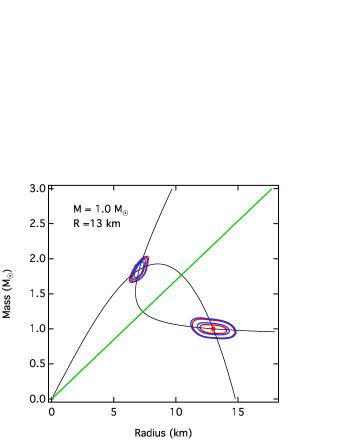
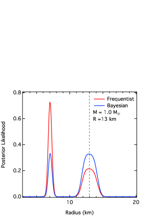
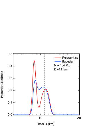
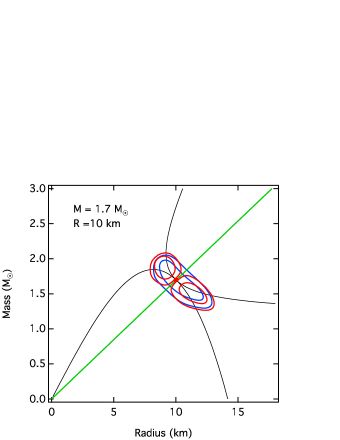
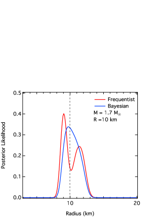
To explore the severity of this bias for a range of neutron star masses and radii, we perform the frequentist inference described above for three different pairs of mock measurements that correspond to stars with different $R/M$ ratios. In all cases, we calculate the apparent angular size and the Eddington flux for the assumed mass and radius of the neutron star by fixing the hydrogen mass fraction to $X=0$, the distance to 4 kpc, and the color correction factor to 1.35. We then assign a 5% Gaussian error in $A$ and $F_{\rm td}$. To infer $R$ and $M$ from these mock measurements, we assume a perfect prior knowledge of the hydrogen mass fraction and distance but take a boxcar prior in the color correction factor between 1.3 and 1.4. The left panels of Figure 1 show the 68% and 95% confidence contours of the posterior likelihood over the inferred mass and radius while the right panels show the posterior likelihood over radius when $P(R,M)$ is marginalized over mass. In the left panels, the black lines correspond to contours of constant $A$ and $F_{\rm td}$ at their central values and for $f_{c}=1.35$, such that one of the intersection of these two lines correspond to the assumed radius. The green line is the critical curve $R=4GM/c^{2}$.

The examples depicted in Figure 1 show that when the assumed value of $R/M$ is significantly away from the critical curve, the posterior likelihood of this frequentist approach is centered on the true solution, with little evidence for bias. However, as the assumed ratio approaches the critical curve, which also corresponds to more realistic values of masses and radii, the inferred radii can be substantially biased toward higher or lower values, by as much as 1.5 km. This is an unacceptably large bias given that $\lesssim 1$ km precision is required in the radius measurements in order to place meaningful constraints on the equation of state (see, e.g., Özel & Psaltis 2009). Moreover, in this idealized example, we assumed that the distance is known with extremely high accuracy, which is unrealistic for the neutron star sources used for the radius measurements. In Section 4, we will explore the effect of realistic distance uncertainties on the radius measurement bias and show that it gets even worse in this frequentist approach. For the measurements performed to date using this approach, this implies that the inferred radii are likely to have been overestimated by $\sim 1-1.5$ km.

Figure 1.— (Left) Contours of 68% and 95% posterior likelihoods over mass and radius using (red) the frequentist and (blue) Bayesian approaches discussed in the text, for three neutron stars with different assumed masses and radii. The true masses and radii are denoted by red filled circles. The black curves correspond to lines of constant apparent angular size, $A$, and Eddington flux, $F_{\rm td}$. The green line corresponds to the critical curve $R=4GM/c^{2}$. (Right) The same posterior likelihoods marginalized over mass. As the true mass and radius of a neutron star approaches the critical curve, the frequentist approach significantly biases the inferred radii. In all cases, the distance of the neutron star was fixed to 4 kpc, the color correction factor to $f_{c}=1.35$, and the hydrogen mass fraction to $X=0$.

3. A NEW BAYESIAN APPROACH TO DETERMINING RADII

The posterior likelihoods over the neutron star mass and radius can be inferred from the same observables $P(A)$ and $P(F_{\rm td})$ in a different way using Bayes’ theorem, according to which

$$P(M,R|{\rm data})=CP(\rm{data}|M,R)P_{\rm pri}(M)P_{\rm pri}(R),$$ (6)

where $P_{\rm pri}(M)$ and $P_{\rm pri}(R)$ are the priors over the mass and radius and $C$ is an appropriate normalization constant. Given that $A$ and $F_{\rm td}$ are ideally uncorrelated measurements, we can write

$$P(\rm{data}|M,R) =\int P(D)\;dD\int P(f_{c})\;df_{c}\int P(X)\;dX$$ (7)

$$\times P[F_{\rm td}(M,R,D)]P[A(M,R,D)].$$

Assuming a flat prior over the radius and mass, it is clear from equations (4) and (7) that the difference between the Bayesian and frequentist inferences discussed here is the presence of the Jacobian in the latter. Consequently, the biases introduced in the frequentist approach by the zero points of the Jacobian are not present here. The underlying reason is that in a Bayesian framework, one does not ask what is the mass and radius pair that corresponds to each set of observables, but rather, for a given mass and radius, what is the chance of obtaining the corresponding set of observables.

In the left panels of Figure 1, we overplot the 68% and 95% confidence contours of the posterior likelihood calculated according to equation 7 and show the marginalized likelihood over the radius in the right panels. When the $R/M$ ratio is significantly away from the critical curve, the Bayesian approach gives unbiased results as in the frequentist approach. There is still a difference between the two approaches, however, which becomes evident in the marginalized likelihoods: the Bayesian approach gives equal maximum likelihood between the two equivalent solutions, whereas the frequentist yields equal integrated likelihoods in the two islands. Given that the two solutions are mathematically equivalent (albeit the smaller radius is sometimes physically unacceptable), the difference in the integrated posterior likelihoods between the two islands should not be used to discriminate between the two solutions.

The biggest difference in the two frameworks occurs when the $R/M$ ratio of neutron stars approach or lie on the critical curve. In these cases, the 68% confidence contour of the Bayesian posterior likelihood encompasses both solutions and, both in the full $P(M,R)$ and in the marginalized $P(R)$ likelihoods, the method results in larger uncertainties in the inference of the radii than in the frequentist approach. However, it does not suffer from the biases of the frequentist approach, which are exacerbated when the neutron stars lie on the critical curve (see the bottom panels of Fig. 1).

4. BIASES IN THE INFERRED EQUATION OF STATE FROM MULTIPLE RADIUS MEASUREMENTS

In the previous sections, we addressed the biases in the inferred radius of a single star using two approaches, a previously developed frequentist and a newly proposed Bayesian formalism, under the assumption of small uncertainties in the two measured quantities $A$ and $F_{\rm td}$. In reality, multiple radius measurements, with different sources of uncertainty, are necessary to place significant constraints on the dense matter equation of state. In this section, we compare the performances of these two approaches under frequentist considerations. In particular, we explore the uncertainties and biases in the inferred properties of the equation of state using mock data sets for multiple objects.

Earlier work has shown that all equations of state that smoothly connect to the low density equation of state of matter can be represented by a small number of parameters, which can be inferred by the measurement of several neutron star radii at different masses (Lindblom 1992; Read et al. 2009; Özel & Psaltis 2009; Gandolfi et al. 2014). In the relevant range of observed neutron-star masses (see, e.g., Özel et al. 2012), most equations of state predict nearly constant radii. For simplicity in the present study, we make use of this fact to reduce the complexity of the equation of state and represent them by a single parameter, which we take to be the constant radius.

Figure 2.— The radius inferred for an equation of state (chosen here to predict constant radius neutron stars over the mass range of interest) using mock spectroscopic observations of five neutron stars, plotted against the assumed radius that it predicts, for a large ensemble of realizations of the mock data, in the (upper) frequentist and (lower) Bayesian approaches discussed in the text. All simulated neutron stars were placed at a distance of 4 kpc and their masses were drawn from a Gaussian distribution that has been inferred observationally for the decendendents of X-ray bursters. The spectroscopic measurements were assumed to have 10% Gaussian errors, while the distance and hydrogen mass fraction was assumed to be accurately known a priori. The frequentist approach leads to substantial biases in the infered radii, while the Bayesian approach does not suffer from biases.

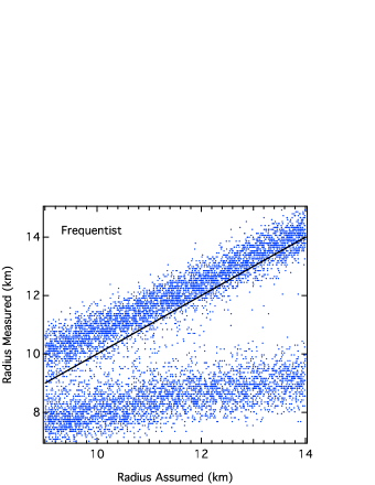
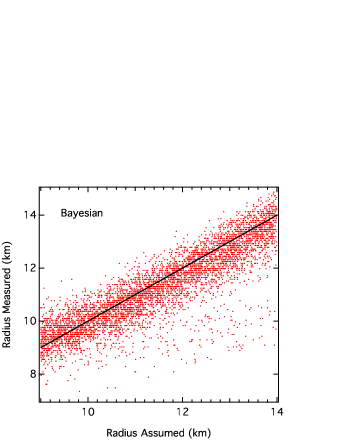
For each assumed neutron star equation of state, and, hence, assumed radius, we draw five neutron star masses from a Gaussian distribution with a mean of $1.46~{}M_{\odot}$ and a dispersion of $0.21~{}M_{\odot}$; this is the distribution of masses that is observationally inferred for the descendants of X-ray bursters (Özel et al. 2012). For each of these neutron stars, we calculate the Eddington flux and the apparent angular size assuming a distance of 4 kpc, color correction factor of 1.35, and a hydrogen mass fraction $X=0$. We assign a 10% Gaussian uncertainty in each of these values, which is typical for X-ray bursters (see Güver et al. 2012 a,b) and draw randomly a set of mock measurements from these distributions. We then apply the frequentist and Bayesian frameworks discussed above to each of these measurements, assuming that the distance and the hydrogen mass fraction are known a priori, but allow the color correction factor to be in the range 1.3-1.4. We marginalize the five resulting posterior likelihoods over mass and then multiply them so that we obtain the posterior likelihood over the inferred radius for that equation of state. We repeat this procedure for 10,000 equations of state with assumed radii between 9 and 14 km and different realizations of the neutron star masses drawn from the same distribution.

Figure 3.— The histogram of the difference between the inferred and assumed radii for two different values of the assumed radius, for the simulated data shown in Figure 2. The bias toward larger radii in the frequentist approach is $\sim 0.75$ km for 12 km neutron stars and $\sim 1$ km for 10 km stars. The proposed Bayesian inference is more accurate but less precise.

In Figure 2, we plot the inferred vs. the assumed radius for each set of mock data for the frequentist and the Bayesian inferences. As expected from the discussion in Section 2, the previously used frequentist inference yields two well separated tracks of solutions, whereas the proposed Bayesian approach has a single band. (Note that the few outliers correspond to the unlikely situations where all five drawn masses are comparable and place the neutron stars away from the critical curve). More importantly, even if the band of small radii is rejected on physical grounds, the remaining band in the frequentist approach yields measured radii that are biased toward larger values. In contrast, the radii inferred in the Bayesian formalism are centered on the assumed values, with little, if any, hints of bias.

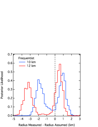
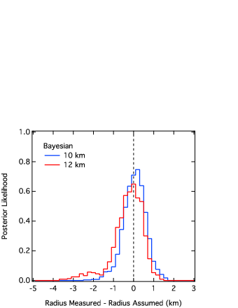
To quantify the degree of bias in these measurements, we plot in Figure 3 the histogram of the difference between the inferred and assumed radii for two different values of the assumed radius. The bias in the frequentist approach (again focusing on the larger of the two solutions) is $+0.75$ km for a 12 km neutron star and $+1$ km for a 10 km neutron star. The histogram in the Bayesian approach, on the other hand, is centered on the true value for both assumed radii, even though it is wider than either of the frequentist peaks. In other words, the frequentist approach generates the more precise but less accurate solution.

The last aspect of the measurements that may bias the inferred radii is how well the distance to the source is known, as reflected in the width of the prior over the distance $P(D)$ that is considered in the calculation. This is of particular concern in the frequentist approach because the Jacobian of the transformation scales as $D^{4}$ and, therefore, places large weight on the smaller distances. We repeated the above simulation of mock observations with two differences. First, we reduced the assumed uncertainties in the measurements of $A$ and $F_{\rm td}$ to 5% in order to focus on the effect of the broader range of distances. Second, even though we placed all simulated neutron stars at 4 kpc, we assumed a flat prior in the distance in the range 3-5 kpc when inferring the radii from the mock measurements.

Figure 4.— Same as Figure 2 but for assumed 5% uncertainties in the spectroscopic measurements and a flat prior in distances in the range 3-5 kpc. In this case, the frequentist approach shows a significant bias toward lower radii, while the Bayesian approach is only marginally affected.

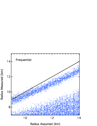
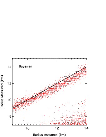
In Figure 4, we plot the inferred vs. the assumed radius for each set of mock data when the range of distances in the priors dominate the uncertainties of the measurement. As in the previous set of mock data, there are two bands of acceptable solutions. However, we will not consider the bands that correspond to small radii any further, as these can typically be rejected on physical grounds. In the frequentist inference, the large range of distance priors biases the inferred radii toward values that are smaller by as much as 1 km than the assumed radii. The reason for this bias is the strong dependence of the Jacobian on distance, which favors the smaller distances and hence the smaller radii. In contrast, the Bayesian inference suffers from a much smaller bias toward smaller radii, even in this case.

5. THE POSTERIOR PROBABILITIES OF THE CONSISTENT MASS-RADIUS SOLUTIONS

In the previous sections, we investigated the biases and uncertainties in the spectroscopically inferred masses and radii of neutron stars within a frequentist and a Bayesian framework. We showed that the fact that real solutions for mass and radius can be obtained for sets of observables that satify $\alpha\leq 1/8$ (see eq. 3) introduces significant biases in this frequentist approach, especially when the true $M,R$ of the neutron star lies near this critical value.

Figure 5.— (Left) The expected distribution over the parameter $\alpha$ calculated for the observed distribution of neutron masses and for several values of the neutron star radius that are within the physically reasonable range. The possible values of $\alpha$ span an extremely narrow range and the likelihood peaks sharply toward the critical value $\alpha=1/8$ for $10-12$ km neutron stars.

We now turn our attention to a second concern arising from the presence of this limit on $\alpha$. In principle, the situation where a set of observables with negligible uncertainties yield $\alpha>1/8$ would imply the inconsistency of the observables and priors with one another. In practice, however, the two observables $F_{\rm td}$ and $A$ have uncertainties and, more importantly, the priors over distance $D$ and the hydrogen mass fraction $X$ are flat over a large range of values. As a result, the range of inferred $\alpha$ values span a wide range, with only a fraction of them falling below the $1/8$ limit. This fraction was used by Steiner et al. (2010) to argue for the inconsistency of observables from some sources; the same argument was later repeated by Miller (2013). We will now use mock data to explore this issue quantitatively and will show the shortcomings of this argument.

We first calculate the expected distribution of $\alpha$ values for realistic neutron star masses and radii. Using equations (1), (2), and (3), we can write $\alpha$ only in terms of $M$ and $R$ as

$$\alpha=\frac{GM}{Rc^{2}}\left(1-\frac{2GM}{Rc^{2}}\right).$$ (8)

If we assume that all neutron stars have the same radius $R_{0}$ in the mass range of interest and masses drawn from the observed distribution of their descendants (i.e., fast pulsars, see §2), then we can write the expected distribution over $\alpha$ as

$$P(\alpha)=P(M)\left|\frac{dM}{d\alpha}\right|.$$ (9)

Equation (8) has two solutions

$$M_{\pm}=\frac{Rc^{2}}{GM}\left(1\pm\sqrt{1-8\alpha}\right)$$ (10)

and, therefore, for $\alpha\leq 1/8$,

$$P(\alpha)=\frac{c^{2}R_{0}}{G\sqrt{1-8\alpha}}\frac{1}{\sqrt{2\pi\sigma^{2}_{M}}}\left[{\rm e}^{-\frac{(M_{-}-M_{0})^{2}}{2\sigma^{2}_{M}}}+{\rm e}^{-\frac{(M_{+}-M_{0})^{2}}{2\sigma^{2}_{M}}}\right]$$ (11)

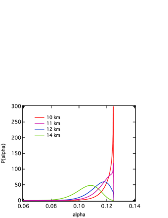
Here, $M_{0}=1.46~{}M_{\odot}$ and $\sigma_{M}=0.21~{}M_{\odot}$ (Özel et al. 2012). We plot in Figure 5 the distribution over $\alpha$ for several physically reasonable neutron star radii.

For radii in the 10-11 km range, the expected distribution over $\alpha$ is very narrowly peaked, with an integrable pole at the limiting value of $\alpha=1/8$. As a result, for such equations of state, obtaining $\alpha$ values from observations that are close to the critical value is, in fact, expected, and cannot be taken as an indication for the inconsistency of the observables, as suggested by Steiner et al. (2010). More importantly, because the two observables $F_{\rm td}$ and $A$ have non-negligible uncertainties and the priors over $D$ and $X$ are typically flat over a wide range of values, the observationally inferred distribution of $\alpha$ will be substantially broader and will very often peak at values $\alpha>1/8$. It then follows that a very large section of the observationally inferred distribution over $\alpha$ will be rejected as leading to unphysical solutions even for favorable uncertainties, without implying an inconsistency among the observables and the priors.

In order to demonstrate this point, we simulate mock data for a $1.7~{}M_{\odot}$, 10 km neutron star placed at a distance of 5 kpc, with a hydrogen mass fraction $X=0$ during Eddington-limited bursts and an atmospheric color correction factor $f_{c}=1.35$. We assign Gaussian 2% uncertainties in the apparent angular size $A$ and in the Eddington flux $F_{\rm td}$; these are comparable to the formal uncertainties reported by Güver et al. (2010a) for 4U 1608$-$52. We then draw Monte Carlo pairs from these two distributions as our mock data for these two quantities. We also take a mock measured distance that is flat between $D_{\rm min}$ and $D_{\max}$ such that the true distance lies between these two values. We also assume, as is sometimes the case, that there is no measurement of the hydrogen mass fraction and we treat is as a flat prior between $X=0$ and $X=0.7$.

The fraction of “accepted” solutions that correspond to $\alpha\leq 1/8$ can be written as an integral over the entire parameter space, limited by the condition

$$\alpha\leq\frac{1}{8}\Rightarrow F_{\rm td}\leq F_{\rm td}^{\rm c}=\frac{c^{3}f_{c}^{2}A^{1/2}}{8k_{\rm 0}(1+X)D}\;.$$ (12)

such that

$$\xi = \frac{1}{2\pi\sigma_{F}\sigma_{A}(D_{\rm max}-D_{\rm min})(X_{\rm max}-X_{\rm min})}$$ (13)

$$\quad\times\int_{D_{\rm min}}^{D_{\rm max}}dD\int_{X_{\rm min}}^{X_{\rm max}}dX\int_{0}^{\infty}dA\int_{0}^{F_{\rm td}^{c}}dF_{\rm td}$$

$$\quad\times\exp\left[-\frac{(A-A_{\rm obs})^{2}}{2\sigma^{2}_{A}}-\frac{(F_{\rm td}-F_{\rm td,obs})^{2}}{2\sigma^{2}_{F}}\right].$$

Here, $A_{\rm obs}$ and $F_{\rm obs}$ are the mock observed data for each realization and we set the observed uncertainties $\sigma_{A}$ and $\sigma_{F}$ equal to the assumed ones; i.e., the measurements do not over- or underestimate the true uncertainties. In the top panel of Figure 6, we show the fraction $\xi$ of acceptable solutions as a function of the upper limit that can be placed on the source distance; for these simulations, we set $D_{\rm min}=4.9$ kpc. Even in the unrealistic case where the distance is extremely well constrained, i.e., $D_{\rm max}-D_{\rm min}\leq 0.2$ kpc, the fraction of accepted solutions is equal to at most a few percent. As the upper bound on the distance increases, the fraction drops to 0.1% or less. Such values are comparable to the ones obtained by Steiner et al. (2010) for 1608$-$52, on which these simulations were based, and show that fractions of this order clearly do not imply any level of inconsistency.

Figure 6.— The fraction of consistent solutions in the frequentist approach as a function of the maximum allowed distance in the distance prior. (Top) The mock data are generated for a $1.7~{}M_{\odot}$, 10 km neutron star assumed to be at 5 kpc and with hydrogen mass fraction $X=0$. They are drawn from Gaussian distributions with 2% uncertainty in in $F_{\rm td}$ and $A$, centered at the true values for the assumed parameters. In the calculation of the fraction of consistent solutions, the priors in the distance and the hydrogen mass fraction are assumed to be flat, spanning the range from 4.9 kpc to $D_{\rm max}$ and 0.0 to 0.7, respectively. The fraction of consistent solutions (see the text for definition) is typically $\sim 1\%$ is known accurately a priori and is dramatically reduced to $\lesssim 0.1\%$ as the upper bound on the source distance increases. (Bottom) Same as above but with true uncertainties in the observables taken to be five times larger than the assumed uncertainties. Underestimating the uncertainties by a factor of 5 reduces the fraction of consistent solutions to as low as $10^{-8}$.

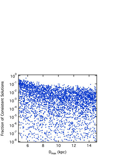
In the bottom panel of Figure 6, we show the results of a similar simulation in which the observational uncertainties are underestimated by a factor of 5; i.e., the dispersions of the distributions used to draw the mock data are 10%, while $\sigma_{A}$ and $\sigma_{F}$ are still set to 2%. We are exploring this situation because the subsequent comprehensive analysis of all the X-ray data from sources that show a large number of thermonuclear bursts indicates a $\simeq 10\%$ spread in the inferred values of $A$ and $F_{\rm td}$ for each source, which is larger than the formal uncertainties of the individual measurements (Güver et al. 2012a, b). In this case, the fraction drops substantially. Steiner et al. (2010) used the similarly low values inferred for 4U 1820$-$30 when only the statistical uncertainties in the data were considered to justify an ad hoc and unphysical reinterpretation of the Eddington limit. This increased the fraction of consistent solutions by artifically moving neutron stars to larger radii and thus, away from the critical value of $\alpha=1/8$. Instead, a correct assessment of the systematic uncertainties in the spectroscopic measurements, as was done in the later studies, provides a much simpler explanation of the inferred small fraction of accepted solutions, without the need for ad hoc reinterpretations of the data.

6. Conclusions

Measuring neutron star radii with spectroscopic and timing techniques requires at least two observed quantities to break the degeneracies between the mass and radius introduced by general relativistic effects. The system of equations that connect the observables to mass and radius often have critical points and regions of no solutions. In this paper, we explored the biases in the inferred radii introduced by this mathematical property of the problem.

We assessed a previously used frequentist method for inferring neutron star radii, devised a new one within a Bayesian framework, and compared their performances under frequentist considerations. We showed that the former suffers from significant biases in the range of masses and radii predicted by the modern equations of state and when realistic uncertainties are taken into account in the measurement of the distance to the source. In contrast, in the latter framework, the inferred uncertainties are larger but the most likely values do not suffer from such biases, making it the preferred framework for measuring neutron star radii using current and future data.

Finally, we explored ways of quantifying the degree of consistency between different spectroscopic measurements from a single source. We demonstrated that the fraction of the parameter space over the observables that gives rise to real solutions in mass and radius is not a good measure of the consistency, as was previously claimed. Fractions of accepted solutions of order 0.1% are common due to the intrinsic uncertainties in the distance and hydrogen mass fraction. In addition, significantly smaller values of the accepted fraction can be accounted for by the recently determined systematic uncertainties in the spectroscopic measurements. In a companion paper, we will apply the statistical framework discussed here to all the currently available spectroscopic measurements of the neutron star radii and constrain the dense matter equation of state.

References

- (1) Bauböck, M., Özel, F., Psaltis, D., & Morsink, S. M. 2015, ApJ, 799, 22
- (2) Feroci, M., Stella, L., van der Klis, M., et al. 2012, Experimental Astronomy, 34, 415
- (3) Gandolfi, S., Carlson, J., Reddy, S., Steiner, A. W., & Wiringa, R. B. 2014, European Physical Journal A, 50, 10
- (4) Gendreau, K. C., Arzoumanian, Z., & Okajima, T. 2012, Proc. SPIE, 8443, 844313
- (5) Güver, T., Özel, F., Cabrera-Lavers, A., & Wroblewski, P. 2010a, ApJ, 712, 964
- (6) Güver, T., Özel, F., & Psaltis, D. 2012a, ApJ, 747, 77
- (7) Güver, T., Psaltis, D., Özel, F. 2012b, ApJ, 747, 76
- (8) Güver, T., Wroblewski, P., Camarota, L., Özel, F. 2010b, ApJ, 719, 1807
- (9) Kuśmierek, K., Madej, J., & Kuulkers, E. 2011, MNRAS, 415, 3344
- (10) Lindblom, L. 1992, ApJ, 398, 569
- (11) Miller, M. C. 2013, arXiv:1312.0029
- (12) Özel, F. 2006, Nature, 441, 1115
- (13) Özel, F., Baym, G., Güver, T. 2010, Phys. Rev. D, 82, 101301
- (14) Özel, F., Güver, T., & Psaltis, D. 2009, ApJ, 693, 1775
- (15) Özel, F., & Psaltis, D. 2009, Phys. Rev. D, 80, 103003
- (16) Özel, F., Psaltis, D., Güver, T., Baym, G., Guillot, S., Heinke, C. 2015, ApJ, submitted, arXiv:1505.05155
- (17) Özel, F., Psaltis, D., Narayan, R., & Santos Villarreal, A. 2012, ApJ, 757, 55
- (18) Paczynski, B. 1983, ApJ, 267, 315
- (19) Psaltis, D., Özel, F., & Chakrabarty, D. 2014, ApJ, 787, 136
- (20) Read, J. S., Lackey, B. D., Owen, B. J., & Friedman, J. L. 2009, Phys. Rev. D, 79, 124032
- (21) Steiner, A. W., Lattimer, J. M., & Brown, E. F. 2010, ApJ, 722, 33
- (22) Suleimanov, V., Poutanen, J., & Werner, K. 2012, A&A, 545, AA120