$B\rightarrow Dl\nu$ form factors at nonzero recoil and extraction of $|V_{cb}|$

Abstract

We present a lattice QCD calculation of the $B\rightarrow Dl\nu$ semileptonic decay form factors $f_{+}(q^{2})$ and $f_{0}(q^{2})$ for the entire physical $q^{2}$ range. Non-relativistic QCD (NRQCD) bottom quarks and Highly Improved Staggered Quark (HISQ) charm and light quarks are employed together with $N_{f}=2+1$ MILC gauge configurations. A joint fit to our lattice and BABAR experimental data allows an extraction of the CKM matrix element $|V_{cb}|$. We also determine the phenomenologically interesting ratio $R(D)={\cal B}(B\rightarrow D\tau\nu_{\tau})/{\cal B}(B\rightarrow Dl\nu_{l})$ ($l=e,\mu$). We find $|V_{cb}|_{excl.}^{B\rightarrow D}=0.0402(17)(13)$, where the first error consists of the lattice simulation errors and the experimental statistical error and the second error is the experimental systematic error. For the branching fraction ratio we find $R(D)=0.300(8)$.

I Introduction

Studies of the heavy-to-heavy semileptonic decays, $B\rightarrow Dl\nu$ and $B_{s}\rightarrow D_{s}l\nu$, lead to a wealth of interesting and important physics. These decays can be used, for example, to extract the Cabibbo-Kobayashi-Maskawa matrix element $|V_{cb}|$, providing an independent check on previous determinations coming from $B\rightarrow D^{*}l\nu$ decays. There is currently a $\sim\,$3$\;\sigma$ tension between the exclusive $|V_{cb}|$ based on $B\rightarrow D^{*}l\nu$ decays at zero recoil and inclusive $|V_{cb}|$ determinations pdg . A recent update DstarMILC by the Fermilab Lattice and MILC collaborations finds $|V_{cb}|^{B\rightarrow D^{*}}_{excl.}=0.03904(49)_{expt.}(53)_{QCD}(19)_{QED}$, whereas the most accurate analysis of inclusive semileptonic decays incvcb gives $|V_{cb}|_{incl.}=0.04221(78)$. The current uncertainty in $|V_{cb}|$ leads to the dominant error in several important Standard Model predictions for rare decays, such as $B_{s}\rightarrow\mu^{+}\mu^{-}$, $K\rightarrow\pi\nu\overline{\nu}$, as well as for the CP violation parameter $\epsilon_{K}$. Reducing this uncertainty will have an impact on precision Flavor Physics.

In order to get more insight into the tension between inclusive and exclusive $|V_{cb}|$ it is crucial to determine $|V_{cb}|_{excl.}$ using channels other than $B\rightarrow D^{*}l\nu$ and also by considering the entire physical $q^{2}$ range, rather than just the zero recoil point. There has been considerable progress on this front. A very recent paper by the Fermilab Lattice and MILC collaborations, using heavy clover bottom and charm quarks, finds $|V_{cb}|_{excl.}^{B\rightarrow D}=(39.6\pm 1.7_{QCD+exp.}\pm 0.2_{QED})\times 10^{-3}$ from $B\rightarrow Dl\nu$ lattice form factors and BABAR data DMILC . And in the present article we give new results on $B\rightarrow Dl\nu$ form factors based on the non-relativistic QCD (NRQCD) action for bottom and the Highly Improved Staggered Quark (HISQ) action for charm quarks. We also combine our lattice form factor results with BABAR data to extract

$$|V_{cb}|_{excl.}^{B\rightarrow D}=0.0402(17)(13),$$ (1)

where the first error comes from the lattice simulation errors and the statistical error from experiment, and the second error is the systematic error from experiment.

Interesting physics may also reside in the ratio $R(D)={\cal B}(B\rightarrow D\tau\nu_{\tau})/{\cal B}(B\rightarrow Dl\nu_{l})$ ($l=\mu$ or $e$). BABAR has reported babar1 an excess in this ratio over Standard Model expectations. The $\tau$ lepton is considerably heavier than the electron or the muon, which means that the branching fraction into $\tau,\nu_{\tau}$ is sensitive to both the vector form factor $f_{+}(q^{2})$ and the scalar form factor $f_{0}(q^{2})$, while the latter does not contribute for decays into $\mu,\nu_{\mu}$ or $e,\nu_{e}$. This could allow scalar contributions from new physics to enter just in the numerator of $R(D)$ and thereby explain the apparent excess. In order to confirm or reject the $R(D)$ anomaly as a true new physics effect, it is important to scrutinize the current Standard Model prediction for $R(D)$. Ref. RdMILC gave the first unquenched lattice result for $R(D)$. Using the new form factors presented in this article we find,

$$R(D)=0.300(8),$$ (2)

the most accurate Standard Model prediction to date.

The rest of this article is organized as follows. Sec. II gives details of the lattice setup for this project, introduces the relevant bottom-charm currents and defines the vector and scalar form factors $f_{+}(q^{2})$ and $f_{0}(q^{2})$. Sec. III introduces the two- and three-point correlators that we simulate and describes our correlator fits and extraction of form factors. In Sec. IV we explain how our results for lattice form factors are extrapolated to the physical, i.e. chiral/continuum, limit. In Sec. V we discuss our form factor results in the physical limit and their errors coming from different sources. We also extract the “slope parameter” $\rho^{2}$ for $f_{+}(q^{2})$. In Sec. VI we combine our Standard Model theory results with experimental measurements of the $B\rightarrow Dl\nu$ branching fraction to extract a new value for $|V_{cb}|$. Sec. VII is devoted to the ratio $R(D)$. We conclude and summarize in Sec. VIII. In Appendix A we provide the relevant information needed to reconstruct our form factors, including correlations. Appendix B discusses further details and checks on the chiral/continuum/kinematic extrapolations. And in Appendix C we list the priors and prior widths used in these extrapolations.

II Lattice Setup and NRQCD/Heavy-HISQ Currents

Table I lists the three coarse ($a\approx 0.12$fm) and two fine ($a\approx 0.09$fm) MILC $N_{f}=2+1$ ensembles latMILC used in this study, together with some further simulation details. These MILC configurations employ the asqtad action to incorporate up, down and strange sea quarks. Compared to our recent $B\rightarrow Kl^{+}l^{-}$ btok1 ; btok2 and $B_{s}\rightarrow Kl\nu$ bstok projects we have increased statistics by about a factor of two or more. For the valence bottom quarks we use the NRQCD action described, for instance, in nrqcd . The valence light and charm quarks are represented by the HISQ action HISQ . In Table II we show the values for valence quark masses. The NRQCD bottom quark mass $aM_{b}$ was tuned in Ref. fb to reproduce the spin averaged $\Upsilon$ mass, whereas the HISQ bare mass $am_{c}$ was tuned to the $\eta_{c}$ mass (suitably modified to accommodate the lack of annihilation and electromagnetic contributions in our simulations) in dtok . The valence HISQ light quark mass $am_{l}$ was chosen to be close to the light asqtad quark mass in the sea.

Table 1: Simulation details on three “coarse” and two “fine” $N_{f}=2+1$ MILC ensembles.

Set	$r_{1}/a$	$m_{l}/m_{s}$ (sea)	$N_{conf}$	$N_{tsrc}$	$L^{3}\times N_{t}$
C1	2.647	0.005/0.050	2096	4	$24^{3}\times 64$
C2	2.618	0.010/0.050	2256	2	$20^{3}\times 64$
C3	2.644	0.020/0.050	1200	2	$20^{3}\times 64$
F1	3.699	0.0062/0.031	1896	4	$28^{3}\times 96$
F2	3.712	0.0124/0.031	1200	4	$28^{3}\times 96$

Table 2: Valence quark masses $aM_{b}$ for NRQCD bottom quarks and $am_{l}$ and $am_{c}$ for HISQ light and charm quarks. The last column gives $Z_{2}^{(0)}(am_{c})$, the tree-level wave function renormalization constant for massive (charm) HISQ quarks matching .

Set	$aM_{b}$	$am_{l}$	$am_{c}$	$Z_{2}^{(0)}(am_{c})$
C1	2.650	0.0070	0.6207	1.00495618
C2	2.688	0.0123	0.6300	1.00524023
C3	2.650	0.0246	0.6235	1.00504054
F1	1.832	0.00674	0.4130	1.00103879
F2	1.826	0.01350	0.4120	1.00102902

To study the process $B\rightarrow D\,l\nu$, one needs to evaluate the matrix element of the bottom-charm charged electroweak current between the $B$ and the $D$ states, $\langle D|(V-A)^{\mu}|B\rangle$. Only the vector current $V^{\mu}$ contributes to the pseudoscalar-to-pseudoscalar amplitude and the matrix element can be written in terms of two form factors $f_{+}(q^{2})$ and $f_{0}(q^{2})$. These depend only on the square of the momentum transfered between the $B$ and the $D$ mesons, $q^{\mu}=p_{B}^{\mu}-p_{D}^{\mu}$,

$$\langle D(p_{D})|V^{\mu}|B(p_{B})\rangle = f_{+}(q^{2})\,\left[p_{B}^{\mu}+p_{D}^{\mu}-\frac{M_{B}^{2}-M_{D}^{2}}{q^{2}}\,q^{\mu}\right]$$ (3)

$$+ f_{0}(q^{2})\;\frac{M_{B}^{2}-M_{D}^{2}}{q^{2}}\;q^{\mu}.$$

Intermediate stages of the analysis are simplified by working with the form factors $f_{\parallel}$ and $f_{\perp}$, defined by

$$\langle D(p_{D})|V^{\mu}|B(p_{B})\rangle=\sqrt{2M_{B}}\,[v^{\mu}f_{\parallel}\,+\,p^{\mu}_{\perp}f_{\perp}],$$ (4)

with

$$v^{\mu}=\frac{p_{B}^{\mu}}{M_{B}},\qquad p_{\perp}^{\mu}=p_{D}^{\mu}-(p_{D}\cdot v)\,v^{\mu}.$$ (5)

In the $B$ rest frame (in this article we only consider $B$ mesons decaying at rest) the temporal and spatial parts of (4) become,

$$\langle D|V^{0}|B\rangle = \sqrt{2M_{B}}\,f_{\parallel},$$ (6)

$$\langle D|V^{k}|B\rangle = \sqrt{2M_{B}}\,p^{k}_{D}\,f_{\perp}.$$ (7)

Hence, one sees that one can separately determine $f_{\parallel}$ or $f_{\perp}$ simply by looking at either the temporal or spatial component of $V^{\mu}$. The conventional form factors $f_{+}(q^{2})$ and $f_{0}(q^{2})$ can then be obtained from

$$f_{+}=\frac{1}{\sqrt{2M_{B}}}\,f_{\parallel}+\frac{1}{\sqrt{2M_{B}}}\,(M_{B}-E_{D})\,f_{\perp},$$ (8)

$$f_{0}=\frac{\sqrt{2M_{B}}}{(M_{B}^{2}-M_{D}^{2})}\,[(M_{B}-E_{D})f_{\parallel}+(E_{D}^{2}-M_{D}^{2})f_{\perp}],$$ (9)

where $E_{D}$ is the daughter $D$ meson energy in the $B$ rest frame. We generate data for four different $D$ meson momenta, $\frac{2\pi}{aL}(0,0,0)$, $\frac{2\pi}{aL}(1,0,0)$, $\frac{2\pi}{aL}(1,1,0)$, and $\frac{2\pi}{aL}(1,1,1)$.

Our goal is to evaluate the hadronic matrix elements $\langle D|V^{0}|B\rangle$ and $\langle D|V^{k}|B\rangle$ via lattice simulations. There are three steps in the calculation. First, one must relate the continuum electroweak currents, $V^{0}$ and $V^{k}$, to lattice operators written in terms of the bottom and charm quark fields in our lattice actions. In the second step the matrix elements of these lattice current operators must be evaluated numerically and the relevant amplitudes, i.e. the matrix elements between the ground state $B$ meson and the ground state $D$ meson with appropriate momenta, must be extracted. This will give us, via Eqs. (6) and (7), the form factors $f_{\parallel}$ and $f_{\perp}$ as functions of the light quark mass and the $D$ momentum. Finally, in step 3 these numerical results must be extrapolated to the physical, chiral/continuum, limit. In the next two sections we describe steps 2 and 3 in turn. Here we consider step 1 and conclude the section with a brief overview of the bottom-charm currents used in our simulations and of how these effective theory currents are matched to those in continuum QCD.

Given our NRQCD action for bottom quarks and HISQ action for charm, we have, through next-to-leading order (NLO) in $1/M$ and lowest order in $\alpha_{s}$, the two currents

$$J^{(0)}_{\mu} = \bar{\psi}_{c}\,\gamma_{\mu}\,\Psi_{b},$$ (10)

$$J^{(1)}_{\mu} = \frac{-1}{2M_{b}}\bar{\psi}_{c}\,\gamma_{\mu}\,\mbox{\boldmath$\gamma\!\cdot\!\nabla$}\,\Psi_{b}.$$ (11)

Here $\psi_{c}$ is the HISQ charm quark field (in its four component “naive fermion” form) and $\Psi_{b}$ the heavy quark field with the upper two components given by the two-component NRQCD fields and the lower two components set equal to zero. We have matched these effective theory currents to $V_{\mu}$ in full QCD at one-loop order through ${\cal O}(\alpha_{s},\frac{\Lambda_{QCD}}{M},\frac{\alpha_{s}}{aM})$. Details of the matching of NRQCD/HISQ currents are given in Ref. matching . The matching is similar to that employed in recent heavy-to-light semileptonic decays (i.e. $B\rightarrow Kl^{+}l^{-}$ and $B_{s}\rightarrow Kl\nu$). However, there is a difference between matching of NRQCD/massless-HISQ and NRQCD/massive-HISQ currents. Massive HISQ fermions have a nontrivial wave function renormalization $Z_{2}^{(0)}$ even at tree-level. To ensure that matching coefficients scale as $\{1+{\cal O}(\alpha_{s})+....\}$, we factor out this tree-level rescaling at the outset. This means the currents in (10) and (11) get multiplied by $\left(Z_{2}^{(0)}\right)^{-1/2}$. After this rescaling, which one sees from Table II is a very small effect, one has

$$\langle V_{\mu}\rangle_{QCD}=(1+\alpha_{s}\,\rho_{\mu})\,\langle J^{(0)}_{\mu}\rangle+\,\langle J^{(1),sub}_{\mu}\rangle,$$ (12)

with

$$J_{\mu}^{(1),sub}=J_{\mu}^{(1)}-\alpha_{s}\,\zeta_{\mu}J_{\mu}^{(0)}.$$ (13)

Here $\rho_{\mu}$ and $\zeta_{\mu}$ are the one-loop matching coefficients tabulated for $\mu=0$ and $\mu=k$ in matching for several $aM_{b}$ and $am_{c}$ values.

III Correlators and Fitting Strategies

In order to extract $\langle D|J_{\mu}|B\rangle$ (here we use “$J_{\mu}$” to denote either the full expression for the current on the rhs of (12) or just the lowest order term $J^{(0)}_{\mu}$), we need to calculate the $B$ and $D$ meson two-point correlators and the $J_{\mu}$ three-point correlator. We use smeared heavy-light bilinears with Coulomb gauge fixed lattices to represent the $B$ meson. For instance, we create a meson at time $t_{0}$ via

$$\Phi^{\alpha\dagger}_{B}(\vec{x},t_{0})\equiv a^{3}\sum_{\vec{x}^{\prime}}\overline{\Psi}_{b}(\vec{x}^{\prime},t_{0})\phi^{\alpha}(\vec{x}^{\prime}-\vec{x})\gamma_{5}\psi_{l}(\vec{x},t_{0}).$$ (14)

For the smearing functions, $\phi^{\alpha}(\vec{x}^{\prime}-\vec{x})$, we use a $\delta$-function local smearing ($\alpha=1$) or Gaussian smearings $\propto e^{-|\vec{x}^{\prime}-\vec{x}|^{2}/(2r_{0}^{2})}$, normalized to one ($\alpha=2$). We then calculate a $2\times 2$ matrix of zero momentum $B$ meson correlators with all combinations of source and sink smearings,

$$C_{B}^{\beta,\alpha}(t,t_{0})=\frac{1}{L^{3}}\sum_{\vec{x},\vec{y}}\langle\Phi_{B}^{\beta}(\vec{y},t)\,\Phi^{\alpha\dagger}_{B}(\vec{x},t_{0})\rangle.$$ (15)

We use Gaussian widths in lattice units of size $r_{0}/a=5$ on coarse ensembles and $r_{0}/a=7$ on the fine ensembles. For the $D$ meson built from HISQ charm and light quarks we use an interpolating operator,

$$\Phi^{\dagger}_{D}(\vec{x},t_{0})=a^{3}\bar{\psi}_{c}(\vec{x},t_{0})\gamma_{5}\psi_{l}(\vec{x},t_{0}),$$ (16)

and construct two-point correlation function with momentum $\vec{p}$,

$$C_{D}(t,t_{0};\vec{p})=\frac{1}{L^{3}}{\cal N}_{taste}\sum_{\vec{x},\vec{y}}e^{i\vec{p}\cdot(\vec{x}-\vec{y})}\langle\Phi_{D}(\vec{y},t)\Phi_{D}^{\dagger}(\vec{x},t_{0})\rangle.$$ (17)

The normalisation factor ${\cal N}_{taste}=1/16$ for four-component naive HISQ quarks, and ${\cal N}_{taste}=1/4$ when employing the one-component version of HISQ. As explained in Ref. heavy_light there are no “taste” related rescaling factors when a nondoubled NRQCD heavy quark propagator is part of the loop, such as in $C_{B}^{\beta,\alpha}(t,t_{0})$ above or in the three-point correlator given below.

The three-point correlator of $J_{\mu}$ can be written as

$$C^{\alpha}_{J}(t,t_{0},T;\vec{p}) = \frac{1}{L^{3}}\sum_{\vec{x},\vec{y},\vec{z}}e^{i\vec{p}\cdot(\vec{z}-\vec{x})}$$

$$\times\langle\Phi_{D}(\vec{x},t_{0}+T)\,J_{\mu}(\vec{z},t)\,\Phi^{\alpha\dagger}_{B}(\vec{y},t_{0})\rangle.$$

The setup for the three-point correlator in (III) is shown in Fig. 1. The $B$ meson is created at time slice $t_{0}$. A current insertion at timeslice $t$, $t_{0}\leq t\leq t_{0}+T$, converts the $b$-quark into a $c$-quark. The resulting $D$ meson is annihilated at timeslice $t_{0}+T$. We have accumulated simulation data for four values of $T$: 12, 13, 14, and 15 on coarse and 21, 22, 23, and 24 on fine lattices. The source time $t_{0}$ is picked randomly for each gauge configuration in order to reduce autocorrelations. Using translational invariance, all data are shifted to $t_{0}=0$ before taking averages and/or doing fits. The spatial sums at the source, $\sum_{\vec{x}}$, in Eqs. (15), (17) and (III) are implemented using $U(1)$ random wall sources $\xi(x^{\prime})$ and $\xi(x)$ (see Ref. dtok for discussions of random wall sources in 2- and three-point correlators).

We fit $C_{B}^{\beta,\alpha}(t)$ to the form

$$C^{\beta,\alpha}_{B}(t) = \sum_{k=0}^{N_{B}-1}b^{\beta}_{k}\,b_{k}^{\alpha*}\,e^{-E^{B,sim}_{k}\cdot t}$$ (19)

$$+\sum_{k=0}^{N_{B}^{\prime}-1}b^{\prime\beta}_{k}\,b_{k}^{\prime\alpha*}\,(-1)^{t}\,e^{-E^{\prime B,sim}_{k}\cdot t}$$

and $C_{D}(t;\vec{p})$ to

$$C_{D}(t,\vec{p}) = \sum_{k=0}^{N_{D}-1}|d_{k}|^{2}(e^{-E^{D}_{k}\cdot t}+e^{-E^{D}_{k}\cdot(N_{t}-t)})$$

$$+ \sum_{k=0}^{N_{D}^{\prime}-1}|d^{\prime}_{k}|^{2}(-1)^{t}(e^{-E^{\prime D}_{k}\cdot t}+e^{-E_{k}^{\prime D}\cdot(N_{t}-t)}).$$

The energy $E^{B,sim}_{k}$ differs from the full energy, $E^{B}_{k}$, because the NRQCD action has the $b$-quark rest mass removed. For the ground state, the two are related by

$$E^{B}_{0}\equiv M_{B}=\frac{1}{2}\left(\overline{M}_{b\overline{b}}^{exp.}-E_{b\overline{b}}^{sim}\right)+E^{B,sim}_{0},$$ (21)

where $\overline{M}_{b\overline{b}}^{exp.}$ is the spin averaged $\Upsilon$ mass used to tune the $b$-quark mass and suitably adjusted as explained in Sec. II. The values of $E^{sim}_{b\overline{b}}$ can be found in Table I of bstok .

By comparing (15) with (19) and (17) with (III), and taking the correct relativistic normalisations for the energy eigenstates $|E^{B}_{k}\rangle$ and $|E^{D}_{k}\rangle$ into account, the following relations emerge,

$$b_{k}^{\alpha*}=\frac{\langle E_{k}^{B}|\Phi_{B}^{\alpha\dagger}|0\rangle}{\sqrt{2a^{3}E_{k}^{B}}},$$ (22)

and

$$d_{k}=\frac{\langle 0|\Phi_{D}|E^{D}_{k}\rangle}{\sqrt{2a^{3}E_{k}^{D}}}.$$ (23)

Figure 1: Setup for three-point correlators

For the three-point correlator $C^{\alpha}_{J}(t,T;\vec{p})$ we use the following fit ansatz

$$C^{\alpha}_{J}(t,T;\vec{p})=\sum_{j=0}^{N_{B}-1}\sum_{k=0}^{N_{D}-1}A^{\alpha}_{jk}e^{-E_{j}^{D}\cdot t}e^{-E_{k}^{B,sim}\cdot(T-t)}$$

$$\quad+\sum_{j=0}^{N_{D}-1}\sum_{k=0}^{N_{B}^{\prime}-1}B^{\alpha}_{jk}e^{-E_{j}^{D}\cdot t}e^{-E_{k}^{\prime B,sim}\cdot(T-t)}(-1)^{(T-t)}$$

$$\quad+\sum_{j=0}^{N_{D}^{\prime}-1}\sum_{k=0}^{N_{B}-1}C^{\alpha}_{jk}e^{-E_{j}^{\prime D}\cdot t}e^{-E_{k}^{B,sim}\cdot(T-t)}(-1)^{t}$$

$$\quad+\sum_{j=0}^{N_{B}^{\prime}-1}\sum_{k=0}^{N_{D}^{\prime}-1}D^{\alpha}_{jk}e^{-E_{j}^{\prime D}\cdot t}e^{-E_{k}^{\prime B,sim}\cdot(T-t)}(-1)^{T}.$$ (24)

The amplitudes $A^{\alpha}_{jk}$ etc. depend on the current $J_{\mu}$ and on the $D$ meson momentum $\vec{p}$. Again by comparing (III) and (III) and using (22) and (23), one finds

$$A^{\alpha}_{jk}=d_{j}\,\frac{\langle E^{D}_{j}|J_{\mu}|E^{B}_{k}\rangle}{\sqrt{2a^{3}E^{D}_{j}}\sqrt{2a^{3}E^{B}_{k}}}\,b^{\alpha*}_{k}.$$ (25)

For $j=k=0$, $A^{\alpha}_{00}$ in (25) gives us the sought after hadronic matrix elements $\langle D|J_{\mu}|B\rangle$,

$$\langle D|J_{\mu}|B\rangle=\frac{A^{\alpha}_{00}}{d_{0}\,b_{0}^{\alpha*}}\,\sqrt{2a^{3}E^{D}_{0}}\,\sqrt{2a^{3}M_{B}}.$$ (26)

Figure 2: $aE_{D}$ versus $N_{exp}$ for several momenta and for ensemble F1.

Figure 3: $aE_{0}^{B,sim}$ versus $N_{exp}$ for ensemble F1.

Figure 4: Dispersion relations on ensembles C1 and F1. The shaded region is bounded by $1\;\pm\;c\,\alpha_{s}\,(ap)^{2}$ with $c=0.1$.

Figure 5: $A_{00}$ for $J_{0}(\vec{p}=(0,0,0))$ versus $N_{D,B}$ and $N^{\prime}_{D,B}$ for F1. The two plots on the right are at fixed $N_{D,B}=4$ or $N^{\prime}_{D,B}=4$.

Figure 6: $A_{00}$ for $J_{0}(\vec{p}=(0,0,0))$ versus different $T$ combinations for F1. We take the result with $T=(21,22,23,24)$.

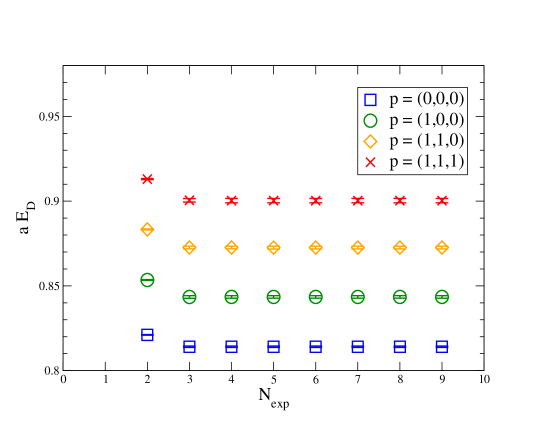
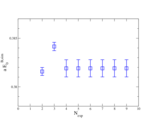
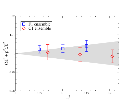
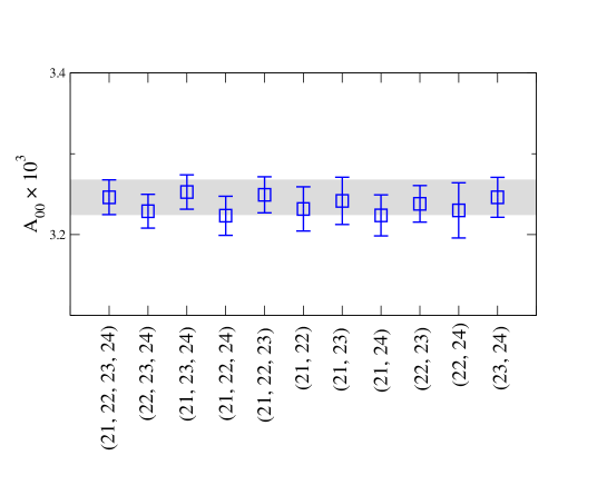
Our fitting strategies based on Bayesian methods have been developed and refined in a number of calculations fit1 ; fit2 . We follow closely the approach used in our recent $B_{s}\rightarrow Kl\nu$ studies bstok . Figs. 2 and 3 show fit results for the groundstate $D$ meson energies $aE_{D}$ and for $aE_{0}^{B,sim}$, respectively, versus the number of exponentials in the fit $N_{exp}$ (we set $N_{exp}=N_{D,B}=N^{\prime}_{D,B}$). Fits stabilize after $N_{exp}=4$. In Fig. 4 we check the ratio $(M^{2}+p^{2})/E^{2}$ for the $D$ meson on one coarse (C1) and one fine (F1) ensemble. The shaded area is bounded by $1\;\pm\;c\>\alpha_{s}(ap)^{2}$, where the free parameter $c$ has been set to $0.1$. One sees that the relativistic dispersion relation holds within errors to better than 0.5%.

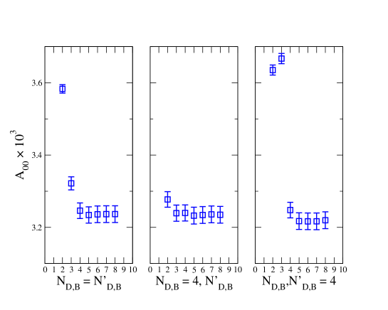
For fixed $D$ momentum, the combination on the rhs of Eq. (24) is obtained from a simultaneous fit to a $2\times 2$ matrix of $B$-correlators, one $D$ correlator and numerous three-point correlators. The number of three-point correlators in the fits varies from six to sixteen as we use either three or four values of $T$, two smearings $\alpha$, and either one current at zero momentum ($J_{0}$) or two currents at non-zero momenta ($J_{0}$ and $J_{i}$). We call this type of fit an “individual fit”. Fig. 5 shows results for $A^{\alpha}_{00}$ for $J_{0}(\vec{p}=(0,0,0))$ versus the number of exponentials. And Fig. 6 shows how results depend on choices for different $T$ combinations. Individual fits give stable and consistent results under such variations.

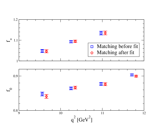
We fit data after the current matching described in Sec. II. Specifically, we obtain simulation data for $J_{\mu}^{(0)}$ and $J_{\mu}^{(1)}$ of Eqs. (8) and (9), reconstruct the full expression on the RHS of Eq (10), and fit the resulting data. Alternatively, we can perform separate fits to $J_{\mu}^{(0)}$ and $J_{\mu}^{(1)}$ and then combine the results according to Eq. (10). We have compared the two approaches and find good agreement, as shown in Fig. 7.

Figure 7: Comparison between form factor fit results when current matching corrections are undertaken before or after the fits (for ensemble F1).

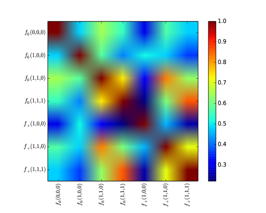
In order to get correlations of form factors at different $q^{2}$’s, one needs to do a simultaneous fit with all different $D$ momenta. Each individual fit alone involves 10 to 20 correlators (depending on the combination of $T$ values) and a simultaneous fit requires a four times larger set of correlators. We find that the simultaneous fits lead to unreliable results, indicating that they are too complicated given the accuracy of our data. Our fitting routines, however, allow for an alternate way to keep track of correlations between form factors at different $q^{2}$’s. One can do a sequence of individual fits, one after the other, all within a single script and always employing the full covariance matrix for all the data (all $D$ meson momenta). We call such fits “master fits”. These master fits are easier than straight simultaneous fits, but still highly non-trivial and time consuming. It was possible to get good master fits consistent with individual fit results; however, these were less stable with respect to changes in $N_{exp}$ and $T$ combinations. Hence for our final fit results we use central values and errors from individual fits, and use the good master fits just to extract the necessary correlations. Fig. 8 shows an example of correlations obtained from a master fit to all the data from ensemble F1. Table III summarizes form factor results for each ensemble and $D$ momentum, and Table IV shows the fit results of $B$ and $D$ meson ground state energies.

Figure 8: Correlations between different momenta from the master fit for ensemble F1.

Table 3: Fit results for $f_{0}(\vec{p})$ and $f_{+}(\vec{p})$.

Set	$f_{0}(0,0,0)$	$f_{0}(1,0,0)$	$f_{0}(1,1,0)$	$f_{0}(1,1,1)$
C1	0.8810(56)	0.8743(43)	0.8608(38)	0.8534(42)
C2	0.8809(31)	0.8716(54)	0.8617(44)	0.8503(50)
C3	0.8872(23)	0.8685(32)	0.8592(29)	0.8473(38)
F1	0.9034(31)	0.8771(42)	0.8643(41)	0.8479(56)
F2	0.9051(23)	0.8895(36)	0.8702(29)	0.8504(34)

Set	$f_{+}(1,0,0)$	$f_{+}(1,1,0)$	$f_{+}(1,1,1)$
C1	1.135(12)	1.1125(57)	1.0837(61)
C2	1.110(12)	1.0809(70)	1.0479(64)
C3	1.1282(71)	1.0937(40)	1.0569(50)
F1	1.1344(91)	1.0931(59)	1.0480(74)
F2	1.1461(72)	1.0963(39)	1.0577(45)

Table 4: Fit results for $aE_{D}$ with each momentum and $aE_{0}^{B,sim}$.

Set	$aE_{D}(0,0,0)$	$aE_{D}(1,0,0)$	$aE_{D}(1,1,0)$	$aE_{D}(1,1,1)$
C1	1.1388(15)	1.1681(19)	1.1979(17)	1.2267(16)
C2	1.1577(14)	1.1959(29)	1.2365(28)	1.2758(34)
C3	1.16355(69)	1.2046(11)	1.2442(12)	1.2824(18)
F1	0.81409(42)	0.84349(77)	0.87262(83)	0.9003(13)
F2	0.81999(37)	0.85051(69)	0.87905(66)	0.90682(86)

Set	$aE_{0}^{B,sim}$
C1	0.4964(13)
C2	0.5089(14)
C3	0.51376(95)
F1	0.38190(89)
F2	0.38726(73)

IV Chiral, Continuum and Kinematic Extrapolation

In this section we describe how we extrapolate the form factors of Table III to the continuum and chiral limits, and how one can get information on the form factors for the entire physical kinematic range. In the continuum physical theory, form factors are functions of a single kinematic variable which can be taken to be $q^{2}$, $E_{D}$, $(w-1)\equiv(q^{2}_{max}-q^{2})/(2M_{B}M_{D})$ or the z-variable defined in terms of $q^{2}$ as,

$$z(q^{2})=\frac{\sqrt{t_{+}-q^{2}}-\sqrt{t_{+}-t_{0}}}{\sqrt{t_{+}-q^{2}}+\sqrt{t_{+}-t_{0}}}.$$ (27)

Here $t_{+}=(M_{B}+M_{D})^{2}$ and $t_{0}$ is a free parameter which we set to $t_{0}=q^{2}_{max}=(M_{B}-M_{D})^{2}\sim 11.66$ GeV². A popular expansion in terms of $z$ is the Bourrely-Caprini-Lellouch (BCL) parametrization bcl , which is given as

$$f_{+}(q^{2})=\frac{1}{P_{+}}\sum_{k=0}^{K-1}a_{k}^{(+)}[z(q^{2})^{k}-(-1)^{k-K}\frac{k}{K}z(q^{2})^{K}]$$ (28)

and,

$$f_{0}(q^{2})=\frac{1}{P_{0}}\sum_{k=0}^{K-1}a_{k}^{(0)}z(q^{2})^{k}.$$ (29)

Here $P_{+,0}$ are the Blaschke factors that take into account the effects of expected poles above the physical region but below the two body threshold $t_{+}$, i.e. in the region $(M_{B}-M_{D})^{2}<q^{2}<(M_{B}+M_{D})^{2}$,

$$P_{+,0}(q^{2})=\left(1-\frac{q^{2}}{M_{+,0}^{2}}\right).$$ (30)

For $f_{+}$ we take the $B_{c}^{*}$ vector meson mass which has been calculated in Ref. bcstar , $M_{+}=M_{B_{c}^{*}}=6.330(9)$GeV. For the scalar form factor $f_{0}$, there is little information theoretically or experimentally on a $0^{+}$ bottom-charm meson. We take $M_{0}$ to be slightly heavier than $M_{+}$ with large errors. We find that our fit results are very insensitive to our choice of $M_{0}$. Even omitting the Blaschke factor completely for $f_{0}(q^{2})$ leads to results consistent with keeping it in (see test number 16 below). The poles in the $B\rightarrow Dl\nu$ form factors are located far above the physical $q^{2}$ region, for example $q^{2}_{max}=(M_{B}-M_{D})^{2}\sim 11.6\;\text{GeV}^{2}$ while $M_{B_{c}^{*}}^{2}\sim 40\;\text{GeV}^{2}$. This implies that the form factors have very small curvatures, and in fact it is very difficult to quantify the curvature for $f_{0}$ from our lattice data.

Once the contributions from simple poles have been isolated, the power series in (28) and (29) correspond to smooth functions of $z$. One reason for prefering a power series in $z$, as opposed to one in $q^{2}$ or $E_{D}$, or even $(w-1)$ is that $|z|$ remains very small throughout the physical kinematic region. For $B\rightarrow D$ semileptonic decays and our choice for $t_{0}$, one has $0.0\leq z<0.064$. This means that one can go to arbitrary high powers in $z^{k}$ if necessary (in practice, with our current simulation data, going up to $z^{3}$ will suffice).

The form factors of Table III are not yet in the physical limit. Nevertheless, for fixed lattice spacing and pion mass, one can again write form factors in terms of a Blaschke factor mutliplying a power series in $z$. The advantages of the z-expansion relative to an expansion in, for instance, powers of $E_{D}$ still hold away from the physical limit. What is different, however, is that expansion coefficients must now depend on the lattice spacing “$a$” and on “$m_{\pi}$” (or the light quark mass),

$$a_{k}^{(0,+)}\rightarrow\tilde{a}_{k}^{(0,+)}\times D_{k}^{(0,+)}(m_{l},m_{l}^{sea},a),$$ (31)

with

$$a_{k}^{(0,+)}=\tilde{a}_{k}^{(0,+)}\times D_{k}^{(0,+)}(m_{l}(phys.),m_{l}^{sea}(phys.),a=0).$$ (32)

This is the modified z-expansion first introduced in Ref.  dtok ; dtopi for $D$ meson semileptonic decays, and which has subsequently also been employed successfully in $B$ and $B_{s}$ meson heavy-to-light decays btok1 ; btok2 ; bstok . The $D_{k}$ in (31) contains all lattice artifacts and chiral logs. Specifically, we have,

$$D_{k} = 1+c_{1}^{k}x_{\pi}+c_{2}^{k}(\frac{1}{2}\delta x_{\pi}+\delta x_{K})+c_{3}^{k}x_{\pi}{\rm log}(x_{\pi})$$ (33)

$$+ d_{1}^{k}(am_{c})^{2}+d_{2}^{k}(am_{c})^{4}$$

$$+ e_{1}^{k}(aE_{D}/\pi)^{2}+e_{2}^{k}(aE_{D}/\pi)^{4},$$

where

$$x_{\pi,K,\eta} = \frac{M_{\pi,K,\eta}^{2}}{(4\pi f_{\pi})^{2}},$$ (34)

$$\delta x_{\pi,K} = \frac{(M_{\pi,K}^{asqtad})^{2}-(M_{\pi,K}^{HISQ})^{2}}{(4\pi f_{\pi})^{2}}.$$ (35)

The $c^{k}_{j}$, with $j=1,2,3$, and $d^{k}_{i}$ and $e^{k}_{i}$, with $i=1,2$, are fit parameters (we have omitted the $f_{+,0}$ label for simplicity) in addition to the $\tilde{a}_{k}^{0,+}$. In Appendix B we discuss what happens when the simple chiral log term in (33) is replaced by expressions from Hard Pion Chiral Perturbation Theory (HPChPT) hpchpt (see also test number 10 below). We list the priors and prior widths used in the chiral/continuum/kinematic extrapolation in Appendix C.

We find it useful to make one more modification of the z-parametrization of lattice form factors. In order to accommodate the uncertainty coming from the truncation of the current matchings at ${\cal O}(\alpha_{s},\Lambda_{QCD}/M,\alpha_{s}/(aM))$, we introduce new fit parameters, $m_{\|}$ and $m_{\bot}$, with central value zero and width $\delta m_{\|,\bot}$,

$$f_{\|},f_{\bot}\rightarrow(1+m_{\|})f_{\|},(1+m_{\bot})f_{\bot}.$$ (36)

The prior widths $\delta m_{\|}$ and $\delta m_{\bot}$ correspond to our best estimates for higher order matching errors for $V_{0}$ and $V_{k}$ respectively. With the modification of (36), our extrapolation results coming from the modified z-expansion fit will then include the matching truncation errors automatically. To get an estimate of higher order matching uncertainties and fix $\delta m_{\|,\bot}$, we have looked at the size of the known first order matching corrections. In other words we have gone through the correlator fits of the previous section once using the fully corrected expression on the rhs of (12) and then a second time using just the lowest order $\langle J^{(0)}_{\mu}\rangle$. We find that the first order matching contributions have only a $\sim 2$% effect on fine and a $\sim 4$% effect on coarse lattices, significantly smaller than a naive $1\times{\cal O}(\alpha)\approx 25-30$% estimate. In this work we take the higher order uncertainties to be the same as the average of the full first order corrections on fine and coarse lattices, that is we set the prior central values and widths of the fit parameters $m_{\|,\bot}$ to be $0.0\pm 0.03$. We have checked that using $0.0\pm 0.02$ or $0.0\pm 0.04$ everywhere, or $0.0\pm 0.02$ for fine and $0.0\pm 0.04$ for coarse lattices has minimal effect (see tests number 13, 14, and 15 below). After the modified z-expansion fits and extrapolation to the physical limit, these matching uncertainties for $f_{\|}$ and $f_{\bot}$ will translate into matching errors for $f_{+}$ and $f_{0}$ with correlations between the two form factors taken into account.

Figure 9: The standard fit results with the continuum extrapolated bands. The short horizontal bars on the upper plot show the fit results at non-zero lattice spacings.

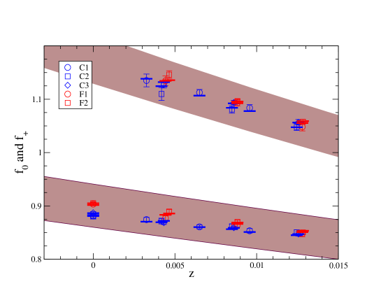
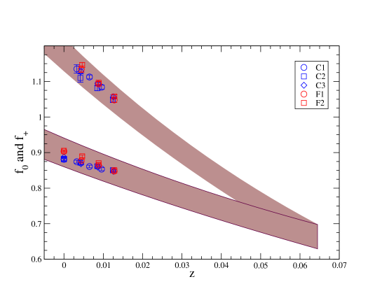
In Fig. 9 we show our fit results for $f_{+}$ and $f_{0}$ plotted versus $z$. We plot both the simulation data and the extrapolated physical band. These are results of what we call our “standard extrapolation” which uses the fit ansatz discussed above and a z-expansion that includes terms through ${\cal O}(z^{3})$. We have carried out further tests of the standard extrapolation by modifying the fit ansatz in the following ways:

1. stop at ${\cal O}(z^{2})$ in the z-expansion;

2. stop at ${\cal O}(z^{4})$ in the z-expansion;

3. add light quark mass dependence to $d_{1}^{k}$ (see Eq. (30) of bstok );

4. add bottom quark mass dependence to $d_{1}^{k}$ (see Eq. (30) of bstok );

5. omit $(am_{c})^{4}$ term;

6. add $(am_{c})^{6}$ term;

7. omit $(aE_{D}/\pi)^{4}$ term;

8. add $(aE_{D}/\pi)^{6}$ term;

9. omit $x{\rm log}(x)$ term;

10. use chiral logs from HPChPT (see Appendix B);

11. add $x_{\pi}^{2}$ term;

12. omit all $x_{i}$ and $x{\rm log}(x)$ terms;

13. use 2% uncertainty for higher order matching contributions;

14. use 4% uncertainty for higher order matching contributions;

15. use 2% uncertainty on fine and 4% uncertainty on coarse lattices for higher order matching contributions;

16. remove Blaschke factor from $f_{0}$ and $f_{+}$.

Figure 10: Test results for $f_{+}(0)$ and $f_{+}(q^{2}_{max})$ under modifications of the “standard extrapolation” fit ansatz. The shaded horizontal bands are the standard extrapolation results. The x-axis labels the modifications 1 - 16 listed in the text.

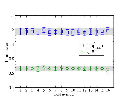
In Fig. 10 we show how results for $f_{+}(q^{2}=0)=f_{0}(0)$ and $f_{+}(q^{2}_{max})$ are affected by these modifications. One sees that our extrapolations are very stable.

V Form Factor Results

Figure 11: Continuum and chiral extrapolated $f_{0}$ (lower band) and $f_{+}$ (upper band).

Figure 12: Relative error components of $f_{0}$ (lower plot) and $f_{+}$ (upper plot) for physical $q^{2}$ region.

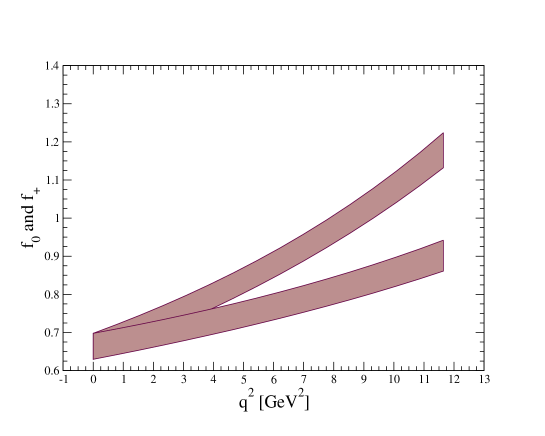
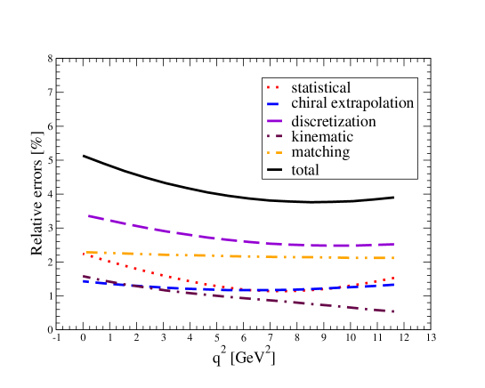
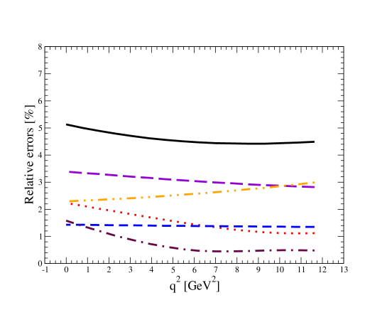
Our final results for the form factors in the physical limit versus $q^{2}$ are shown in Fig. 11. Error plots for $f_{+}(q^{2})$ and $f_{0}(q^{2})$ are given in Fig. 12. We isolate the errors coming from different sources and also give the total error as a function of $q^{2}$. The individual errors in Fig. 12 correspond to the following:

• statistical
  The statistical error includes the three and two-point correlator fit errors and the scale errors ($r_{1}$ and $r_{1}/a$). These are lattice simulation errors, and we have lattice data in the large $q^{2}$ region, from about $9.5~{}\text{GeV}^{2}$ to $12~{}\text{GeV}^{2}$. Fig. 12 shows the propagation of such errors to the continuum limit and after extrapolation to the full $q^{2}$ range.

• chiral extrapolation
  These are the valence and sea quark mass extrapolation errors including effects of chiral logs. They come from the fit parameters $c^{k}_{1}$, $c^{k}_{2}$ and $c^{k}_{3}$ in Eq. (33).

• discretization
  Discretization errors come from the $(am_{c})^{n}$ and $(aE_{D})^{n}$ terms and they constitute the dominant errors in our calculation.

• kinematic
  These come from the z-expansion coefficients $\tilde{a}^{(0,+)}_{k}$ and the pole locations. As one would expect, the error increases as $q^{2}$ decreases.

• matching
  Matching errors come from the $m_{\perp,\parallel}$ fit parameters as explained in the previous section.

Physical meson mass input errors (0.01%) and finite size errors (0.1%) are not included in the plots, since they are too small to have any effect.

The slope of $f_{+}(q^{2})$ as one comes down from the zero recoil point at $q^{2}=q^{2}_{max}$ is a quantity that is often quoted when comparing different measurements of this form factor. In terms of the variable $w=(M_{B}^{2}+M_{D}^{2}-q^{2})/(2M_{B}M_{D})$ the slope parameter $\rho^{2}$ is given by

$${\cal G}(w)={\cal G}(1)\;\left\{1-\rho^{2}(w-1)+{\cal O}((w-1)^{2})\right\},$$ (37)

where,

$${\cal G}(w=w(q^{2}))=\frac{2\sqrt{\kappa}}{1+\kappa}f_{+}(q^{2})$$ (38)

for

$$\kappa=\frac{M_{D}}{M_{B}}.$$ (39)

A popular way to extract $\rho^{2}$ is to use the Caprini-Lellouch-Neubert (CLN) parametrization cln ,

$${\cal G}(w) = {\cal G}(1)\;\left\{1-8\rho^{2}z+(51\rho^{2}-10)z^{2}\right.$$ (40)

$$\left.\qquad\qquad\quad-(252\rho^{2}-84)z^{3}\right\},$$

with,

$$z=\frac{\sqrt{w+1}-\sqrt{2}}{\sqrt{w+1}+\sqrt{2}}.$$ (41)

This “$z$” is the same as the z-variable introduced in the previous section, Eq. (27), with the same $t_{0}=q^{2}_{max}$. Using Eq. (40), we extract

$$\rho^{2}=1.119(71),\qquad\qquad{\cal G}(1)=1.035(40).$$ (42)

Another useful reference point is the value of $f_{+}(0)=f_{0}(0)$. We find,

$$f_{+}(0)=0.664(34).$$ (43)

In Appendix A we provide the z-expansion coefficients including errors and correlations for the form factors of Fig. 11.

VI Extraction of $|V_{cb}|$

The differential branching fraction for $B\rightarrow Dl\nu$ decays is given by,

$$\frac{d\Gamma}{dq^{2}}=\eta_{EW}\frac{G_{F}^{2}|V_{cb}|^{2}}{24\pi^{3}M_{B}^{2}}(1-\frac{m_{l}^{2}}{q^{2}})^{2}|\vec{p}|$$

$$\times \left[(1+\frac{m_{l}^{2}}{2q^{2}})M_{B}^{2}|\vec{p}|^{2}f_{+}^{2}(q^{2})+\frac{3m_{l}^{2}}{8q^{2}}(M_{B}^{2}-M_{D}^{2})^{2}f_{0}^{2}(q^{2})\right],$$

where $m_{l}$ is the mass of the lepton, and $\eta_{EW}$ is the electro-weak correction. The main goal of the present work is to combine experimental measurement of this differential branching fraction with form factors of the previous section to extract $|V_{cb}|$. The partial branching fraction (the left hand side of Eq. VI) has been measured by BABAR babar2010 . On the right hand side, we have form factors from this lattice calculation, and all other factors are known except the target quantity $|V_{cb}|$.

In order to include the higher order electro-weak effects, we apply the Sirlin factor sirlin , $\eta_{s}=1.00662$. Furthermore, there are final state electro-magnetic interactions for the neutral channel, $\bar{B}^{0}\rightarrow D^{+}l\nu$, which we estimate to be a less than 0.5% effect using the signal yield ratio of the charged and neutral decay channels. Combining the two effects, we get $\eta_{EW}=1.011(5)$.

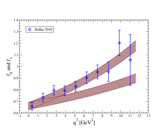
We perform another modified z-expansion fit explained in Sec. IV together with the BABAR experiment data with $|V_{cb}|$ as a fit parameter. We have a good fit with $\chi^{2}/dof=0.88$, and this is shown in Fig. 13. We get $|V_{cb}|$ from this fit,

$$|V_{cb}|=0.0402(17)(13),$$ (45)

where the first error is from the fit including all lattice errors and experimental statistical errors, and the second error is the experimental systematic error. We quote the experimental systematic errors as 3.3% of our fit result based on BABAR’s estimate of their systematic errors in babar2010 . This is equivalent to imposing 3.3% systematic errors on each experimental measurement bin with 100% correlations.

Figure 13: Form factors using both lattice and BABAR  babar2010 inputs, together with the experimental data points.

A detailed error budget is shown in Table V. The dominant errors are experimental systematic, lattice discretization, and operator matching errors. Thus, improvements in both experiments and lattice calculations are required to obtain better precision on $|V_{cb}|$ from our method.

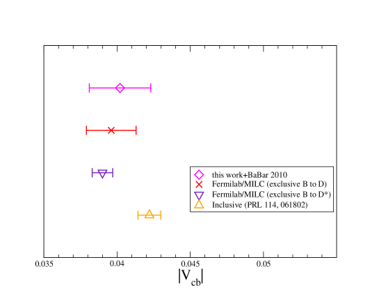
$|V_{cb}|$ has been reported from multiple lattice and non-lattice calculations. We compare the different determinations in Fig. 14. Our result agrees with other exclusive calculations, particularly with the most accurate result from $B\rightarrow D^{*}l\nu$, but it is also compatible within errors with the inclusive determination. Since the discretization error is one of the dominant errors in our calculation, lattice errors can be reduced in the future by working on more ensembles with finer lattice spacings.

Table 5: Error budget table for $|V_{cb}|$. The first three rows are from experiments, and the rest are from lattice simulations.

Type	Partial errors [%]
experimental statistics	1.55
experimental systematic	3.3
meson masses	0.01
lattice statistics	1.22
chiral extrapolation	1.14
discretization	2.59
kinematic	0.96
matching	2.11
electro-weak	0.48
finite size effect	0.1
total	5.34

Figure 14: $|V_{cb}|$ comparisons between inclusive and exclusive determinations.

VII The R(D) Ratio

The experimental data used in the previous section to extract $|V_{cb}|$ were for semileptonic decays with light leptons in the final state. BABAR has also studied decays involving the much heavier $\tau$ lepton, $B\rightarrow D\tau\nu_{\tau}$, and measured the ratio,

$$R(D)=\frac{{\cal B}(B\rightarrow D\tau\nu_{\tau})}{{\cal B}(B\rightarrow Dl\nu)},$$ (46)

where $l$ is either an electron or a muon. They find

$$R(D)|_{exp.}=0.440(58)(42),$$ (47)

where the first error is the statistical and the second is the systematic error rdbabar .

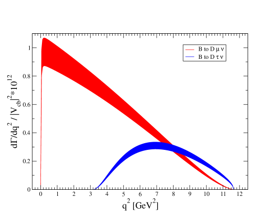
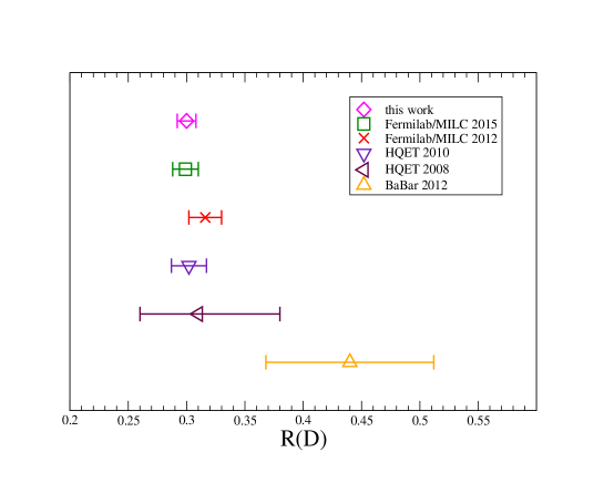
Here we present a Standard Model prediction for $R(D)$ based on our new form factors. Fig. 15 compares differential branching fractions of Eq. (VI) for $B\rightarrow D\tau\nu_{\tau}$ and for $B\rightarrow Dl\nu$. Although only $f_{+}(q^{2})$ contributes to the $l\nu$ case, both $f_{+}(q^{2})$ and $f_{0}(q^{2})$ are involved in the $\tau\nu_{\tau}$ branching fraction. Integrating over $q^{2}$ we obtain,

$$R(D)|_{SM}=0.300(8).$$ (48)

Table VI shows a detailed error budget for $R(D)$. Fig. 16 gives a comparison plot for different determinations of $R(D)$. All Standard Model based calculations are in good agreement with each other. The difference between our result and experiment is at the $2\sigma$ level. We note that we do not use any experimental results to extract $R(D)$. Our result gives the most accurate pure Standard Model prediction to date for $R(D)$.

Table 6: Error budget table for $R(D)$.

Type	Partial errors [%]
lattice statistics	1.24
chiral extrapolation	0.28
discretization	1.08
kinematic	1.61
matching	1.03
finite size effect	0.1
total	2.54

Figure 15: The differential branching fractions for $B\rightarrow Dl\nu$ and $B\rightarrow D\tau\nu$

Figure 16: Comparisons between different determinations of $R(D)$. The references for the other determinations are BABAR 2012 rdbabar , HQET 2008 rdhqet2 , HQET 2010 rdhqet , Fermilab/MILC 2012 RdMILC , and Fermilab/MILC 2015 DMILC .

VIII Summary and Future Prospects

In this paper we have presented a new lattice QCD calculation of the $B\rightarrow Dl\nu$ semileptonic decay form factors $f_{+}(q^{2})$ and $f_{0}(q^{2})$. These were combined with experimental measurements of differential branching fractions to extract a value for $|V_{cb}|_{excl.}$. Our result, given in Eq. (1) (and repeated in (45)) is consistent with other recent lattice determinations using different lattice actions, and provides a cross check of earlier calculations. We summarize these results in Fig. 14.

The dominant error in our calculation is the discretization error, followed by higher order current matching uncertainties. The former error can be reduced by adding simulation data from further ensembles with finer lattice spacings. We are also exploring ways to improve our matching errors by combining simulations with NRQCD bottom-quarks with those employing heavier than charm HISQ quarks. This approach to nonperturbative matchings of NRQCD/HISQ currents is described briefly in the Appendix to Ref. bstok . There we presented ratios of $B_{s}\rightarrow Kl\nu$ and $B_{s}\rightarrow\eta_{s}l\nu$ form factors and explained how such ratios combined with a purely HISQ calculation in the future of $B_{s}\rightarrow\eta_{s}l\nu$ form factors would lead to a nonperturbative determination of the NRQCD/HISQ bottom-up current Z-factors. Similarly, nonperturbative Z-factors for bottom-charm currents used in the present calculation could be obtained by calculating $B_{s}\rightarrow D_{s}l\nu$ forms factors once with NRQCD bottom-quarks and then again with heavy-HISQ bottom-quarks and then taking ratios. We have already completed, and are in the process of writing up, calculations of $B_{s}\rightarrow D_{s}l\nu$ form factors with NRQCD bottom-quarks. Simulations with heavy-HISQ bottom-quarks are also underway. Hence we expect to be able to significantly reduce theory errors in $|V_{cb}|$ determinations from $B\rightarrow Dl\nu$ decays in the near future. In the meantime we hope that experimental measurements will also improve considerably. Only then will one be able to shed light on the exclusive versus inclusive tensions for $|V_{cb}|$ via studies of $B\rightarrow Dl\nu$ decays.

In this article we also determined the ratio $R(D)$. Our result is given in Eq. (2) (and again in (48)). We summarize comparisons between Standard Model predictions and experiment in Fig. 16. It will be interesting to see whether the current $\sim$2$\sigma$ tension will develop into a true discrepancy between experiment and the Standard Model or disappear.

Acknowledgements:
H. N. is supported in part by the U.S. Department of Energy (DOE) under Grant No. DE-FC02-12ER41879 and by the U.S. National Science Foundation (NSF) under Grant No. PHY10-034278; C. M. B. and J. S. by U.S. DOE under Grant No. DE-SC0011726 and C. M. by U.S. NSF under Grant No. PHY10-034278. Numerical simulations were carried out on facilities of the USQCD collaboration funded by the Office of Science of the DOE and at the Ohio Supercomputer Center. We thank the MILC collaboration for use of their gauge configurations.

Appendix A Reconstructing Form Factors

We provide our z-expansion coefficients with correlations, so that readers can reconstruct our form factors for their analysis. The form factors are expressed by the BCL parameterization as

$$f_{+}(q^{2})=\frac{1}{P_{+}}\sum_{k=0}^{2}a_{k}^{(+)}[z(q^{2})^{k}-(-1)^{k-K}\frac{k}{K}z(q^{2})^{K}],$$ (49)

and

$$f_{0}(q^{2})=\frac{1}{P_{0}}\sum_{k=0}^{2}a_{k}^{(0)}z(q^{2})^{k},$$ (50)

where

$$z(q^{2}) = \frac{\sqrt{t_{+}-q^{2}}-\sqrt{t_{+}-t_{0}}}{\sqrt{t_{+}-q^{2}}+\sqrt{t_{+}-t_{0}}},$$ (51)

$$t_{+} = (M_{B}+M_{D})^{2},$$ (52)

$$t_{0} = q^{2}_{max}=(M_{B}-M_{D})^{2},$$ (53)

$$P_{+,0}(q^{2}) = \left(1-\frac{q^{2}}{M_{+,0}^{2}}\right).$$ (54)

For the locations of the poles, one can use $M_{+}=6.330(9)$ GeV for $f_{+}$, and $M_{0}=6.420(9)$ GeV for $f_{0}$ to reproduce our form factors exactly. The coefficients, $a_{k}^{(+,0)}$, and the correlations are presented in Table VII.

Table 7: z-expansion coefficients and its covariance.

coefficient	value
$a_{0}^{(0)}$	0.647(29)
$a_{1}^{(0)}$	0.27(30)
$a_{2}^{(0)}$	-0.09(2.94)
$a_{0}^{(+)}$	0.836(33)
$a_{1}^{(+)}$	-2.66(52)
$a_{2}^{(+)}$	-0.07(2.96)

	$a_{0}^{(0)}$	$a_{1}^{(0)}$	$a_{2}^{(0)}$	$a_{0}^{(+)}$	$a_{1}^{(+)}$	$a_{2}^{(+)}$
$a_{0}^{(0)}$	8.442e-4	-1.141e-3	-5.072e-3	4.799e-4	3.801e-3	5.518e-3
$a_{1}^{(0)}$		9.255e-2	-1.087e-1	5.390e-4	5.835e-2	1.852e-2
$a_{2}^{(0)}$			8.652	6.813e-3	2.504e-1	2.402e-1
$a_{0}^{(+)}$				1.062e-3	-7.548e-3	-7.354e-3
$a_{1}^{(+)}$					2.747e-01	-3.561e-1
$a_{2}^{(+)}$						8.740

Appendix B Chiral/Continuum Extrapolations using Input from HPChPT

In the standard extrapolation of Sec. IV we used a generic $c^{k}_{3}x_{\pi}{\rm log}(x_{\pi})$ term to parametrize chiral logarithmic contributions and allowed $c^{k}_{3}$ to float. An alternate way to introduce chiral logarithms into our chiral/continuum extrapolations is to use expressions fixed by hard pion chiral perturbation theory (HPChPT) hpchpt ,

$$[\text{logs}]_{f_{+}} = -\,\frac{\kappa+1}{\sqrt{\kappa}}\frac{g^{2}}{(4\pi f_{\pi})^{2}}(r(w)-1)$$ (55)

$$\times\;\left(\frac{3}{2}\bar{A}(x_{\pi})+\bar{A}(x_{K})+\frac{1}{6}\bar{A}(x_{\eta})\right),$$

$$[\text{logs}]_{f_{0}} = -\frac{\sqrt{\kappa}}{1+\kappa}\frac{g^{2}}{(4\pi f_{\pi})^{2}}(w+1)\,(r(w)-1)$$ (56)

$$\times\;\left(\frac{3}{2}\bar{A}(x_{\pi})+\bar{A}(x_{K})+\frac{1}{6}\bar{A}(x_{\eta})\right),$$

where

$$\bar{A}(x) = x\,{\rm log}(x),$$ (57)

$$w = \frac{M_{B}^{2}+M_{D}^{2}-q^{2}}{2M_{B}M_{D}},$$ (58)

$$r(w) = \frac{1}{\sqrt{w^{2}-1}}{\rm log}(w+\sqrt{w^{2}-1}),$$ (59)

$$\kappa = M_{D}/M_{B}.$$ (60)

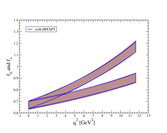
We find very consistent results for the extrapolated physical form factors using either generic $c^{k}_{3}$ terms or (55) & (56). This is already evident in Fig. 10 test number 10 for $f_{+}(0)$ and $f_{+}(q^{2}_{max})$. In Fig. 17 we compare the two approaches over the entire $q^{2}$ range.

Figure 17: Comparison between using a generic $x_{\pi}{\rm log}(x_{\pi})$ term (filled blocks) and chiral logarithms from HPChPT (open blocks).

Appendix C Priors and Prior Widths for the Chiral/Continuum/Kinematic Extrapolation

In earlier works dtok ; dtopi , we split the priors for the modified z-expansion method into two groups: Group I and Group II. The Group I parameters are typical fit parameters, such as quark mass dependence or z-expansion parameters. In this work, the Group I parameters consist of

$$c_{1}^{k},c_{2}^{k},c_{3}^{k},d_{1}^{k},d_{2}^{k},e_{1}^{k},e_{2}^{k},a_{k},$$ (61)

where $k=0,1,$ and $2$, and there are two sets of parameters for each $f_{0}$ and $f_{+}$ form factors. These parameters are defined in Eq. (28), (29), and (33), and the priors and fit results are shown in Table VIII.

We choose priors as following. For the valence quark mass terms, $c_{1}^{k}$, we use $0.0(1.0)$, since the mass terms are normalized by the scale, $4\pi f_{\pi}$. However, it is well-known that the sea quark mass effects are smaller than those of the valence quark effects, so we take $0.0(3)$ for the sea quark mass terms, $c_{2}^{k}$. HPChPT suggests a prior for the generic chiral log term, $x_{\pi}log(x_{\pi})$, as $0.0(1)$. This prior essentially covers variations of the terms on entire kinematic range. For more conservative error estimations, we take $0.0(2)$ as our prior for the generic chiral log term. We note that the prior settings with $0.0(1)$ and $0.0(2)$ give almost identical results. In the HISQ action, leading heavy quark discretization errors are ${\cal O}(\alpha_{s}v^{2}/c^{2}am_{c}^{2})$ and ${\cal O}(v^{2}/c^{2}am_{c}^{4})$. We conservatively do not take the $v^{2}/c^{2}$ terms in our power counting, so that we take $0.0(3)$ for $d_{1}^{k}$ and $e_{1}^{k}$ priors, and $0.0(1.0)$ for $d_{2}^{k}$ and $e_{2}^{k}$ priors. For the priors for z-expansion coefficients, $a_{k}^{(+,0)}$, we searched for broad enough priors that gave stable fit results, and we take $0.0(3.0)$ in this work.

Table 8: Priors and fit results of the Group I parameters for the modified z-expansion fit.

Group I	prior [$f_{0}$]	fit result [$f_{0}$]	prior [$f_{+}$]	fit result [$f_{+}$]
$c_{1}^{0}$	0.0 (1.0)	-0.09 (18)	0.0 (1.0)	0.34 (20)
$c_{1}^{1}$	0.0 (1.0)	-0.13 (99)	0.0 (1.0)	-0.67 (87)
$c_{1}^{2}$	0.0 (1.0)	0.0 (1.0)	0.0 (1.0)	0.0 (1.0)
$c_{2}^{0}$	0.00 (30)	0.03 (28)	0.00 (30)	-0.10 (28)
$c_{2}^{1}$	0.00 (30)	0.00 (30)	0.00 (30)	-0.01 (30)
$c_{2}^{2}$	0.00 (30)	0.00 (30)	0.00 (30)	0.00 (30)
$c_{3}^{0}$	0.00 (20)	-0.10 (15)	0.00 (20)	0.22 (16)
$c_{3}^{1}$	0.00 (20)	0.006 (200)	0.00 (20)	0.03 (20)
$c_{3}^{2}$	0.00 (20)	-0.00 (20)	0.00 (20)	0.00 (20)
$d_{1}^{0}$	0.00 (30)	-0.16 (24)	0.00 (30)	0.11 (24)
$d_{1}^{1}$	0.00 (30)	0.02 (30)	0.00 (30)	-0.005 (292)
$d_{1}^{2}$	0.00 (30)	-0.00 (30)	0.00 (30)	0.00 (30)
$d_{2}^{0}$	0.0 (1.0)	-0.17 (44)	0.0 (1.0)	-0.29 (40)
$d_{2}^{1}$	0.0 (1.0)	0.2 (1.0)	0.0 (1.0)	0.008 (923)
$d_{2}^{2}$	0.0 (1.0)	-0.0 (1.0)	0.0 (1.0)	0.0 (1.0)
$e_{1}^{0}$	0.00 (30)	0.21 (25)	0.00 (30)	0.06 (25)
$e_{1}^{1}$	0.00 (30)	0.008 (300)	0.00 (30)	-0.005 (298)
$e_{1}^{2}$	0.00 (30)	0.00 (30)	0.00 (30)	0.00 (30)
$e_{2}^{0}$	0.0 (1.0)	1.44 (66)	0.0 (1.0)	0.03 (82)
$e_{2}^{1}$	0.0 (1.0)	0.02 (1.00)	0.0 (1.0)	0.0 (1.0)
$e_{2}^{2}$	0.0 (1.0)	0.0 (1.0)	0.0 (1.0)	0.0 (1.0)
$a_{0}$	0.0 (3.0)	0.644 (30)	0.0 (3.0)	0.842 (35)
$a_{1}$	0.0 (3.0)	0.27 (31)	0.0 (3.0)	-2.69 (54)
$a_{2}$	0.0 (3.0)	-0.09 (2.94)	0.0 (3.0)	-0.07 (2.96)

The Group II parameters are

$$\left(\frac{r_{1}}{a}\right)^{i},aM_{B}^{i},aE_{D}^{i}(\vec{p}),aM_{\pi}^{i},(aM_{K}^{asqtad})^{i},(aM_{\pi}^{asqtad})^{i},$$

$$M_{0},M_{+},r_{1},M_{\pi}^{phys},M_{K}^{phys},M_{B}^{phys},M_{D}^{phys},$$ (62)

where $i$ is the index for the five ensembles ($i=1,2,3,4,$ and $5$). The Group II parameters are either from experiments, from other lattice simulations, or from the correlator fits, and used for input parameters. The prior settings and fit results for the Group II are shown in Table IX and X.

Table 9: Priors and fit results of the Group II parameters for the modified z-expansion fit. Parameters with five rows are lattice quantities for the five ensembles, C1, C2, C3, F1, and F2.

Group II	prior	fit result
$r_{1}/a$	2.6470 (30)	2.6473 (30)
	2.6180 (30)	2.6174 (30)
	2.6440 (30)	2.6442 (30)
	3.6990 (30)	3.6991 (30)
	3.7120 (40)	3.7120 (39)
$aM_{B}$	3.18915 (65)	3.18905 (65)
	3.23184 (88)	3.23197 (87)
	3.21191 (77)	3.21177 (77)
	2.28109 (52)	2.28092 (50)
	2.28101 (44)	2.28105 (44)
$aE_{D}$	1.1389 (10)	1.13894 (82)
$\vec{p}=(0,0,0)$	1.15993 (82)	1.16011 (80)
	1.16339 (54)	1.16333 (54)
	0.81452 (35)	0.81444 (35)
	0.81993 (27)	0.81997 (27)
$aE_{D}$	1.1688 (11)	1.16827 (88)
$\vec{p}=(1,0,0)$	1.19901 (99)	1.19918 (94)
	1.20395 (77)	1.20445 (69)
	0.84360 (58)	0.84374 (52)
	0.85071 (40)	0.85055 (39)
$aE_{D}$	1.19884 (84)	1.19847 (80)
$\vec{p}=(1,1,0)$	1.24003 (87)	1.23982 (83)
	1.24485 (78)	1.24477 (71)
	0.87300 (62)	0.87299 (57)
	0.87885 (36)	0.87890 (35)
$aE_{D}$	1.22775 (96)	1.22746 (94)
$\vec{p}=(1,1,1)$	1.27839 (93)	1.27825 (91)
	1.28321 (94)	1.28319 (89)
	0.90004 (78)	0.90027 (70)
	0.90627 (49)	0.90630 (46)

Table 10: (Continued) Priors and fit results of the Group II parameters for the modified z-expansion fit. Parameters with five rows are lattice quantities for the five ensembles, C1, C2, C3, F1, and F2.

Group II	prior	fit result
$aM_{\pi}$	0.15990 (20)	0.15990 (20)
	0.21110 (20)	0.21110 (20)
	0.29310 (20)	0.29310 (20)
	0.13460 (10)	0.13460 (10)
	0.18730 (10)	0.18730 (10)
$aM_{K}^{asqtad}$	0.36530 (29)	0.36530 (29)
	0.38331 (24)	0.38331 (24)
	0.40984 (21)	0.40984 (21)
	0.25318 (19)	0.25318 (19)
	0.27217 (21)	0.27217 (21)
$aM_{\pi}^{asqtad}$	0.15971 (20)	0.15971 (20)
	0.22447 (17)	0.22447 (17)
	0.31125 (16)	0.31125 (16)
	0.14789 (18)	0.14789 (18)
	0.20635 (18)	0.20635 (18)
$M_{0}$	6.53 (1.00)	6.42(43)
$M_{+}$	6.3300 (90)	6.3300(90)
$r_{1}$	0.3133 (23)	0.3132 (23)
$M_{\pi}^{phys}$	0.1373 (23)	0.1373 (23)
$M_{K}^{phys}$	0.4957 (20)	0.4957 (20)
$M_{B}^{phys}$	5.27942 (17)	5.27942 (17)
$M_{D}^{phys}$	1.86690 (40)	1.86690 (40)

References

- (1) K. Olive et al. (Particle Data Group), Chin. Phys. C38, 090001 (2014).
- (2) J. Bailey et al. (Fermilab/MILC), Phys. Rev. D 89 (2014) 114504.
- (3) A. Alberti, P. Gambino, K.J. Healey, and S. Nandi, Phys. Rev. Lett. 114 (2015) 061802, [arXiv:1411.6560 [hep-ph]].
- (4) J. Bailey et al. (Fermilab/MILC), arXiv:1503.07237.
- (5) J. P. Lees et al. (BABAR), Phys. Rev. D 88 (2013) 072012.
- (6) J. Bailey et al. (Fermilab/MILC), Phys. Rev. Lett. 109 (2012) 071802.
- (7) A. Bazavov et al. (MILC), Rev. Mod. Phys. 82 (2010) 1349.
- (8) C. Bouchard, G. P. Lepage, C. Monahan, H. Na, and J. Shigemitsu (HPQCD), Phys. Rev. Lett. 111 (2013) 162002.
- (9) C. Bouchard, G. P. Lepage, C. Monahan, H. Na, and J. Shigemitsu (HPQCD), Phys. Rev. D 88 (2013) 054509.
- (10) C. Bouchard, G. P. Lepage, C. Monahan, H. Na, and J. Shigemitsu (HPQCD), Phys. Rev. D 90 (2014) 054506.
- (11) G. P. Lepage, L. Magnea, C. Nakhleh, U. Magnea, and K. Hornbostel (HPQCD), Phys. Rev. D 46 (1992) 4052.
- (12) E. Follana, Q. Mason, C. Davies, K. Hornbostel, G. P. Lepage, J. Shigemitsu, H. Trottier, and K. Wong (HPQCD), Phys. Rev. D 75 (2007) 054502.
- (13) H. Na, C. Monahan, C. T. H. Davies, R. Horgan, G. P. Lepage, and J. Shigemitsu (HPQCD), Phys. Rev. D 86 (2012) 034506.
- (14) H. Na, C. T. H. Davies, E. Follana, G. P. Lepage, and J. Shigemitsu (HPQCD), Phys. Rev. D 82 (2010) 114506.
- (15) C. Monahan, J. Shigemitsu, and R. Horgan (HPQCD), Phys. Rev. D 87 (2013) 034017.
- (16) M. Wingate, J. Shigemitsu, C. T. H. Davies, G. P. Lepage, and Howard D. Trottier (HPQCD), Phys. Rev. D 67 (2003) 054505.
- (17) G. P. Lepage, B. Clark, C T. H. Davies, K. Hornbostel, P. B. Mackenzie, C. Morningstar, H. Trottier (HPQCD), Nucl. Phys. Proc. Suppl. 106 (2002) 12.
- (18) K. Hornbostel, G. P. Lepage, C. T. H. Davies, R. J. Dowdall, H. Na, and J. Shigemitsu (HPQCD), Phys. Rev. D 85 (2012) 031504.
- (19) C. Bourrely, L. Lellouch, and I. Caprini, Phys. Rev. D 79 (2009) 013008.
- (20) E. B. Gregory, C. T. H. Davies, E. Follana, E. Gamiz, I. D. Kendall, G. P. Lepage, H. Na, J. Shigemitsu, and K. Y. Wong (HPQCD), Phys. Rev. Lett. 104 (2010) 022001.
- (21) H. Na, C. T. H. Davies, E. Follana, J. Koponen, G. P. Lepage, and J. Shigemitsu (HPQCD), Phys. Rev. D 84 (2011) 114505.
- (22) J. Bijnens and I. Jemos, Nucl. Phys. B 846 (2011) 145.
- (23) I. Caprini, L. Lellouch, M. Neubert, Nucl. Phys. B530 (1998) 153.
- (24) B. Aubert et al. [BABAR Collaboration], Phys. Rev. Lett. 104, 011802 (2010) [arXiv:0904.4063 [hep-ex]].
- (25) D. Atwood and W. J. Marciano, Phys. Rev. D 41 (1990) 1736.
- (26) J. P. Lees et al. [BABAR Collaboration], Phys. Rev. Lett. 109 (2012) 101802 [arXiv:1205.5442 [hep-ex]].
- (27) U. Nierste, S. Trine and S. Westhoff, Phys. Rev. D 78 (2008) 015006. [arXiv:0801.4938 [hep-ph]].
- (28) M. Tanaka and R. Watanabe, Phys. Rev. D 82 (2010) 034027.