Mind the duality gap: safer rules for the Lasso

Abstract

Screening rules allow to early discard irrelevant variables from the optimization in Lasso problems, or its derivatives, making solvers faster. In this paper, we propose new versions of the so-called safe rules for the Lasso. Based on duality gap considerations, our new rules create safe test regions whose diameters converge to zero, provided that one relies on a converging solver. This property helps screening out more variables, for a wider range of regularization parameter values. In addition to faster convergence, we prove that we correctly identify the active sets (supports) of the solutions in finite time. While our proposed strategy can cope with any solver, its performance is demonstrated using a coordinate descent algorithm particularly adapted to machine learning use cases. Significant computing time reductions are obtained with respect to previous safe rules.

1 Introduction

Since the mid 1990’s, high dimensional statistics has attracted considerable attention, especially in the context of linear regression with more explanatory variables than observations: the so-called $p>n$ case. In such a context, the least squares with $\ell_{1}$ regularization, referred to as the Lasso (Tibshirani, 1996) in statistics, or Basis Pursuit (Chen et al., 1998) in signal processing, has been one of the most popular tools. It enjoys theoretical guarantees (Bickel et al., 2009), as well as practical benefits: it provides sparse solutions and fast convex solvers are available. This has made the Lasso a popular method in modern data-science toolkits. Among successful fields where it has been applied, one can mention dictionary learning (Mairal, 2010), bio-statistics (Haury et al., 2012) and medical imaging (Lustig et al., 2007; Gramfort et al., 2012) to name a few.

Many algorithms exist to approximate Lasso solutions, but it is still a burning issue to accelerate solvers in high dimensions. Indeed, although some other variable selection and prediction methods exist (Fan & Lv, 2008), the best performing methods usually rely on the Lasso. For stability selection methods (Meinshausen & Bühlmann, 2010; Bach, 2008; Varoquaux et al., 2012), hundreds of Lasso problems need to be solved. For non-convex approaches such as SCAD (Fan & Li, 2001) or MCP (Zhang, 2010), solving the Lasso is often a required preliminary step (Zou, 2006; Zhang & Zhang, 2012; Candès et al., 2008).

Among possible algorithmic candidates for solving the Lasso, one can mention homotopy methods (Osborne et al., 2000), LARS (Efron et al., 2004), and approximate homotopy (Mairal & Yu, 2012), that provide solutions for the full Lasso path, i.e., for all possible choices of tuning parameter $\lambda$. More recently, particularly for $p>n$, coordinate descent approaches (Friedman et al., 2007) have proved to be among the best methods to tackle large scale problems.

Following the seminal work by El Ghaoui et al. (2012), screening techniques have emerged as a way to exploit the known sparsity of the solution by discarding features prior to starting a Lasso solver. Such techniques are coined safe rules when they screen out coefficients guaranteed to be zero in the targeted optimal solution. Zeroing those coefficients allows to focus more precisely on the non-zero ones (likely to represent signal) and helps reducing the computational burden. We refer to (Xiang et al., 2014) for a concise introduction on safe rules. Other alternatives have tried to screen the Lasso relaxing the “safety”. Potentially, some variables are wrongly disregarded and post-processing is needed to recover them. This is for instance the strategy adopted for the strong rules (Tibshirani et al., 2012).

The original basic safe rules operate as follows: one chooses a fixed tuning parameter $\lambda$, and before launching any solver, tests whether a coordinate can be zeroed or not (equivalently if the corresponding variable can be disregarded or not). We will refer to such safe rules as static safe rules. Note that the test is performed according to a safe region, i.e., a region containing a dual optimal solution of the Lasso problem. In the static case, the screening is performed only once, prior any optimization iteration. Two directions have emerged to improve on static strategies.

• The first direction is oriented towards the resolution of the Lasso for a large number of tuning parameters. Indeed, practitioners commonly compute the Lasso over a grid of parameters and select the best one in a data-driven manner, e.g., by cross-validation. As two consecutive $\lambda^{\prime}s$ in the grid lead to similar solutions, knowing the first solution may help improve screening for the second one. We call sequential safe rules such strategies, also referred to as recursive safe rules in (El Ghaoui et al., 2012). This road has been pursued in (Wang et al., 2013; Xu & Ramadge, 2013; Xiang et al., 2014), and can be thought of as a “warm start” of the screening (in addition to the warm start of the solution itself). When performing sequential safe rules, one should keep in mind that generally, only an approximation of the previous dual solution is computed. Though, the safety of the rule is guaranteed only if one uses the exact solution. Neglecting this issue, leads to “unsafe” rules: relevant variables might be wrongly disregarded.

• The second direction aims at improving the screening by interlacing it throughout the optimization algorithm itself: although screening might be useless at the beginning of the algorithm, it might become (more) efficient as the algorithm proceeds towards the optimal solution. We call these strategies dynamic safe rules following (Bonnefoy et al., 2014a, b).

Based on convex optimization arguments, we leverage duality gap computations to propose a simple strategy unifying both sequential and dynamic safe rules. We coined GAP SAFE rules such safe rules.

The main contributions of this paper are 1) the introduction of new safe rules which demonstrate a clear practical improvement compared to prior strategies 2) the definition of a theoretical framework for comparing safe rules by looking at the convergence of their associated safe regions.

In Section 2, we present the framework and the basic concepts which guarantee the soundness of static and dynamic screening rules. Then, in Section 3, we introduce the new concept of converging safe rules. Such rules identify in finite time the active variables of the optimal solution (or equivalently the inactive variables), and the tests become more and more precise as the optimization algorithm proceeds. We also show that our new GAP SAFE rules, built on dual gap computations, are converging safe rules since their associated safe regions have a diameter converging to zero. We also explain how our GAP SAFE tests are sequential by nature. Application of our GAP SAFE rules with a coordinate descent solver for the Lasso problem is proposed in Section 4. Using standard data-sets, we report the time improvement compared to prior safe rules.

1.1 Model and notation

We denote by $[d]$ the set $\{1,\ldots,d\}$ for any integer $d\in\mathbb{N}$. Our observation vector is $y\in\mathbb{R}^{n}$ and the design matrix $X=[x_{1},\cdots,x_{p}]\in\mathbb{R}^{n\times p}$ has $p$ explanatory variables (or features) column-wise. We aim at approximating $y$ as a linear combination of few variables $x_{j}$’s, hence expressing $y$ as $X\beta$ where $\beta\in\mathbb{R}^{p}$ is a sparse vector. The standard Euclidean norm is written $\|\cdot\|$, the $\ell_{1}$ norm $\|\cdot\|_{1}$, the $\ell_{\infty}$ norm $\|\cdot\|_{\infty}$, and the matrix transposition of a matrix $Q$ is denoted by ${Q}^{\top}$. We denote $(t)_{+}=\max(0,t)$.

For such a task, the Lasso is often considered (see Bühlmann & van de Geer (2011) for an introduction). For a tuning parameter $\lambda>0$, controlling the trade-off between data fidelity and sparsity of the solutions, a Lasso estimator $\hat{\beta}^{({\lambda})}$ is any solution of the primal optimization problem

$$\hat{\beta}^{({\lambda})}\in\mathop{\mathrm{arg\,min}}_{\beta\in\mathbb{R}^{p}}\underbrace{\frac{1}{2}\left\lVert X\beta-y\right\rVert_{2}^{2}+\lambda\left\lVert\beta\right\rVert_{1}}_{=P_{\lambda}(\beta)}\enspace.$$ (1)

Denoting $\Delta_{X}=\big{\{}\theta\in\mathbb{R}^{n}\;:\;\left\lvert x_{j}^{\top}\theta\right\rvert\leq 1,\forall j\in[p]\big{\}}$ the dual feasible set, a dual formulation of the Lasso reads (see for instance Kim et al. (2007) or Xiang et al. (2014)):

$$\hat{\theta}^{({\lambda})}=\mathop{\mathrm{arg\,max}}_{\theta\in\Delta_{X}\subset\mathbb{R}^{n}}\underbrace{\frac{1}{2}\left\lVert y\right\rVert^{2}_{2}-\frac{\lambda^{2}}{2}\left\lVert\theta-\frac{y}{\lambda}\right\rVert^{2}_{2}}_{=D_{\lambda}(\theta)}.$$ (2)

We can reinterpret Eq. (2) as $\hat{\theta}^{({\lambda})}=\Pi_{\Delta_{X}}(y/\lambda)$, where $\Pi_{\mathcal{C}}$ refers to the projection onto a closed convex set $\mathcal{C}$. In particular, this ensures that the dual solution $\hat{\theta}^{({\lambda})}$ is always unique, contrarily to the primal $\hat{\beta}^{({\lambda})}$.

Rule	Center	Radius	Ingredients
Static Safe (El Ghaoui et al., 2012)	$y/\lambda$	$\widecheck{R}_{\lambda}(\frac{y}{\lambda_{\max}})$	$\lambda_{\max}=\|X^{\top}y\|_{\infty}\!=\!|x_{j^{\star}}^{\top}y|$
Dynamic ST3 (Xiang et al., 2011)	$y/\lambda-\delta x_{j^{\star}}\!$	$(\widecheck{R}_{\lambda}(\theta_{k})^{2}-\delta^{2})^{\frac{1}{2}}$	$\delta=\left(\frac{\lambda_{\max}}{\lambda}-1\right)/\|x_{j^{\star}}\|^{2}$
Dynamic Safe (Bonnefoy et al., 2014a)	$y/\lambda$	$\widecheck{R}_{\lambda}(\theta_{k})$	$\theta_{k}\in\Delta_{X}$ (e.g., as in (11) )
Sequential (Wang et al., 2013)	$\hat{\theta}^{({\lambda_{t-1}})}$	$\left|\frac{1}{\lambda_{t-1}}-\frac{1}{\lambda_{t}}\right|\|y\|$	exact $\hat{\theta}^{({\lambda_{t-1}})}$ required
GAP SAFE sphere (proposed)	$\theta_{k}$	${r}_{\lambda_{t}}(\beta_{k},\theta_{k})=\frac{1}{\lambda_{t}}\sqrt{2G_{\lambda_{t}}(\beta_{k},\theta_{k})}$	dual gap for $\beta_{k},\theta_{k}$

Table 1: Review of some common safe sphere tests.

1.2 A KKT detour

For the Lasso problem, a primal solution $\hat{\beta}^{({\lambda})}\in\mathbb{R}^{p}$ and the dual solution $\hat{\theta}^{({\lambda})}\in\mathbb{R}^{n}$ are linked through the relation:

$$y=X\hat{\beta}^{({\lambda})}+\lambda\hat{\theta}^{({\lambda})}\enspace.$$ (3)

The Karush-Khun-Tucker (KKT) conditions state:

$$\forall j\in[p],\;x_{j}^{\top}\hat{\theta}^{({\lambda})}\in\begin{cases}\{\operatorname{sign}(\hat{\beta}^{({\lambda})}_{j})\}&\,\text{if}\quad\hat{\beta}^{({\lambda})}_{j}\neq 0,\\ [-1,1]&\,\text{if}\quad\hat{\beta}^{({\lambda})}_{j}=0.\\ \end{cases}$$ (4)

See for instance (Xiang et al., 2014) for more details. The KKT conditions lead to the fact that for $\lambda\geq\lambda_{\max}=\|X^{\top}y\|_{\infty}$, $0\in\mathbb{R}^{p}$ is a primal solution. It can be considered as the mother of all safe screening rules. So from now on, we assume that $\lambda\leq\lambda_{\max}$ for all the considered $\lambda$’s.

2 Safe rules

Safe rules exploit the KKT condition (4). This equation implies that $\hat{\beta}^{({\lambda})}_{j}=0$ as soon as $|x_{j}^{\top}\hat{\theta}^{({\lambda})}|<1$. The main challenge is that the dual optimal solution is unknown. Hence, a safe rule aims at constructing a set $\mathcal{C}\subset\mathbb{R}^{n}$ containing $\hat{\theta}^{({\lambda})}$. We call such a set $\mathcal{C}$ a safe region. Safe regions are all the more helpful that for many $j$’s, $\mu_{\mathcal{C}}(x_{j}):=\sup_{\theta\in\mathcal{C}}|x_{j}^{\top}\theta|<1$, hence for many $j$’s, $\hat{\beta}^{({\lambda})}_{j}=0$.

Practical benefits are obtained if one can construct a region $\mathcal{C}$ for which it is easy to compute its support function, denoted by $\sigma_{\mathcal{C}}$ and defined for any $x\in\mathbb{R}^{n}$ by:

$$\sigma_{\mathcal{C}}(x)=\max_{\theta\in\mathcal{C}}~{}x^{\top}\theta\,.$$ (5)

Cast differently, for any safe region $\mathcal{C}$, any $j\in[p]$, and any primal optimal solution $\hat{\beta}^{({\lambda})}$, the following holds true:

$$\text{If }\mu_{\mathcal{C}}(x_{j})=\max(\sigma_{\mathcal{C}}(x_{j}),\sigma_{\mathcal{C}}(-x_{j}))<1\text{ then }\hat{\beta}^{({\lambda})}_{j}\!=0.$$ (6)

We call safe test or safe rule, a test associated to $\mathcal{C}$ and screening out explanatory variables thanks to Eq. (6).

Remark 1.

Reminding that the support function of a set is the same as the support function of its closed convex hull (Hiriart-Urruty & Lemaréchal, 1993)[Proposition V.2.2.1], we restrict our search to closed convex safe regions.

Based on a safe region $\mathcal{C}$ one can partition the explanatory variables into a safe active set $A^{\lambda}(\mathcal{C})$ and a safe zero set $Z^{\lambda}(\mathcal{C})$ where:

$$A^{(\lambda)}(\mathcal{C})=\{j\in[p]:\mu_{\mathcal{C}}(x_{j})\geq 1\},$$ (7)

$$Z^{(\lambda)}(\mathcal{C})=\{j\in[p]:\mu_{\mathcal{C}}(x_{j})<1\}.$$ (8)

Note that for nested safe regions $\mathcal{C}_{1}\subset\mathcal{C}_{2}$ then $A^{(\lambda)}(\mathcal{C}_{1})\subset A^{(\lambda)}(\mathcal{C}_{2})$. Consequently, a natural goal is to find safe regions as small as possible: narrowing safe regions can only increase the number of screened out variables.

Remark 2.

If $\mathcal{C}=\{\hat{\theta}^{({\lambda})}\}$, the safe active set is the equicorrelation set $A^{(\lambda)}(\mathcal{C})=\mathcal{E}_{\lambda}:=\{j\in[p]:|x_{j}^{\top}\hat{\theta}^{({\lambda})}|=1\}$ (in most cases (Tibshirani, 2013) it is exactly the support of $\hat{\beta}^{({\lambda})}$). Even when the Lasso is not unique, the equicorrelation set contains all the solutions’ supports. The other extreme case is when $\mathcal{C}=\Delta_{X}$, and $A^{(\lambda)}(\mathcal{C})=[p]$. Here, no variable is screened out: $Z^{(\lambda)}(\mathcal{C})=\emptyset$ and the screening is useless.

We now consider common safe regions whose support functions are easy to obtain in closed form. For simplicity we focus only on balls and domes, though more complicated regions could be investigated (Xiang et al., 2014).

2.1 Sphere tests

Following previous work on safe rules, we call sphere tests, tests relying on balls as safe regions. For a sphere test, one chooses a ball containing $\hat{\theta}^{({\lambda})}$ with center $c$ and radius $r$, i.e., $\mathcal{C}=B(c,r)$. Due to their simplicity, safe spheres have been the most commonly investigated safe regions (see for instance Table 1 for a brief review). The corresponding test is defined as follows:

$$\text{If }\mu_{B(c,r)}(x_{j})=|x_{j}^{\top}c|+r\|x_{j}\|<1,\text{ then }\hat{\beta}^{({\lambda})}_{j}=0.$$ (9)

Note that for a fixed center, the smaller the radius, the better the safe screening strategy.

Example 1.

The first introduced sphere test (El Ghaoui et al., 2012) consists in using the center $c=y/\lambda$ and radius $r=|1/\lambda-1/\lambda_{\max}|\|y\|$. Given that $\hat{\theta}^{({\lambda})}=\Pi_{\Delta_{X}}(y/\lambda)$, this is a safe region since $y/\lambda_{\max}\in\Delta_{X}$ and $\|y/\lambda_{\max}-\Pi_{\Delta_{X}}(y/\lambda)\|\leq\|y\||1/\lambda-1/\lambda_{\max}|$. However, one can check that this static safe rule is useless as soon as

$$\frac{\lambda}{\lambda_{\max}}\leq\min_{j\in[p]}\left(\frac{1+|x_{j}^{\top}y|/(\|x_{j}\|\|y\|)}{1+\lambda_{\max}/(\|x_{j}\|\|y\|)}\right).$$ (10)

2.2 Dome tests

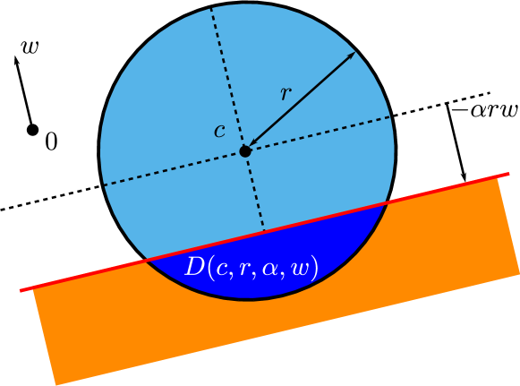
Other popular safe regions are domes, the intersection between a ball and a half-space. This kind of safe region has been considered for instance in (El Ghaoui et al., 2012; Xiang & Ramadge, 2012; Xiang et al., 2014; Bonnefoy et al., 2014b). We denote $D(c,r,\alpha,w)$ the dome with ball center $c$, ball radius $r$, oriented hyperplane with unit normal vector $w$ and parameter $\alpha$ such that $c-\alpha rw$ is the projection of $c$ on the hyperplane (see Figure 1 for an illustration in the interesting case $\alpha>0$).

Remark 3.

The dome is non-trivial whenever $\alpha\in[-1,1]$. When $\alpha=0$, one gets simply a hemisphere.

For the dome test one needs to compute the support function for $\mathcal{C}=D(c,r,\alpha,w)$. Interestingly, as for balls, it can be obtained in a closed form. Due to its length though, the formula is deferred to the Appendix (see also (Xiang et al., 2014)[Lemma 3] for more details).

Figure 1: Representation of the dome $D(c,r,\alpha,w)$ (dark blue). In our case, note that $\alpha$ is positive.

2.3 Dynamic safe rules

For approximating a solution $\hat{\beta}^{({\lambda})}$ of the Lasso primal problem $P_{\lambda}$, iterative algorithms are commonly used. We denote $\beta_{k}\in\mathbb{R}^{p}$ the current estimate after $k$ iterations of any iterative algorithm (see Section 4 for a specific study on coordinate descent). Dynamic safe rules aim at discovering safe regions that become narrower as $k$ increases. To do so, one first needs dual feasible points: $\theta_{k}\in\Delta_{X}$. Following El Ghaoui et al. (2012) (see also (Bonnefoy et al., 2014a)), this can be achieved by a simple transformation of the current residuals $\rho_{k}=y-X\beta_{k}$, defining $\theta_{k}$ as

$$\begin{cases}\theta_{k}\!=\!{\alpha}_{k}\rho_{k},\\ \alpha_{k}\!=\!\min\!\Big{[}\!\max\!\left(\frac{y^{\top}\!\rho_{k}}{\lambda\left\lVert\rho_{k}\right\rVert^{2}},\!\frac{-1}{\left\lVert X^{\top}\rho_{k}\right\rVert_{\infty}}\right)\!\!,\!\frac{1}{\left\lVert X^{\top}\rho_{k}\right\rVert_{\infty}}\Big{]}.\\ \end{cases}$$ (11)

Such dual feasible $\theta_{k}$ is proportional to $\rho_{k}$, and is the closest point (for the norm $\|\cdot\|$) to $y/\lambda$ in $\Delta_{X}$ with such a property, i.e., $\theta_{k}=\Pi_{\Delta_{X}\cap\operatorname{Span}(\rho_{k})}(y/\lambda)$. A reason for choosing this dual point is that the dual optimal solution $\hat{\theta}^{({\lambda})}$ is the projection of $y/\lambda$ on the dual feasible set $\Delta_{X}$, and the optimal $\hat{\theta}^{({\lambda})}$ is proportional to $y-X\hat{\beta}^{({\lambda})}$, cf. Equation (3).

Remark 4.

Note that if $\lim_{k\to+\infty}\beta_{k}=\hat{\beta}^{({\lambda})}$ (convergence of the primal) then with the previous display and (3), we can show that $\lim_{k\to+\infty}\theta_{k}=\hat{\theta}^{({\lambda})}$. Moreover, the convergence of the primal is unaltered by safe rules: screening out unnecessary coefficients of $\beta_{k}$, can only decrease the distance between $\beta_{k}$ and $\hat{\beta}^{({\lambda})}$.

Example 2.

Note that any dual feasible point $\theta\in\Delta_{X}$ immediately provides a ball that contains $\hat{\theta}^{({\lambda})}$ since

$$\left\lVert\hat{\theta}^{({\lambda})}-\frac{y}{\lambda}\right\rVert=\min_{\theta^{\prime}\in\Delta_{X}}\left\lVert\theta^{\prime}-\frac{y}{\lambda}\right\rVert\leq\left\lVert\theta-\frac{y}{\lambda}\right\rVert:=\widecheck{R}_{\lambda}(\theta).$$ (12)

The ball $B\big{(}y/\lambda,\widecheck{R}_{\lambda}(\theta_{k})\big{)}$ corresponds to the simplest safe region introduced in (Bonnefoy et al., 2014a, b) (cf. Figure 2 for more insights). When the algorithm proceeds, one expects that $\theta_{k}$ gets closer to $\hat{\theta}^{({\lambda})}$, so $\|\theta_{k}-y/\lambda\|$ should get closer to $\|\hat{\theta}^{({\lambda})}-y/\lambda\|$. Similarly to Example 1, this dynamic rule becomes useless once $\lambda$ is too small. More precisely, this occurs as soon as

$$\frac{\lambda}{\lambda_{\max}}\leq\min_{j\in[p]}\left(\frac{1+|x_{j}^{\top}y|/(\|x_{j}\|\|y\|)}{\lambda_{\max}\|\hat{\theta}^{({\lambda})}\|/\|y\|\\ +\lambda_{\max}/(\|x_{j}\|\|y\|)}\right).$$ (13)

Noticing that $\|\hat{\theta}^{({\lambda})}\|\leq\|y/\lambda\|$ (since $\Pi_{\Delta_{X}}$ is a contraction and $0\in\Delta_{X}$) and proceeding as for (10), one can show that this dynamic safe rule is inefficient when:

$$\frac{\lambda}{\lambda_{\max}}\leq\min_{j\in[p]}\left(\frac{|x_{j}^{\top}y|}{\lambda_{\max}}\right).$$ (14)

This is a critical threshold, yet the screening might stop even at a larger $\lambda$ thanks to Eq. (13). In practice the bound in Eq. (13) cannot be evaluated a priori due to the term $\|\hat{\theta}^{({\lambda})}\|$). Note also that the bound in Eq. (14) is close to the one in Eq. (10), explaining the similar behavior observed in our experiments (see Figure 3 for instance).

(a) Location of the dual optimal $\hat{\theta}^{({\lambda})}$ in the annulus.

(b) Refined location of the dual optimal $\hat{\theta}^{({\lambda})}$ (dark blue).

(c) Proposed GAP SAFE sphere (orange).

(d) Proposed GAP SAFE dome (orange).

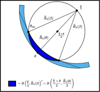
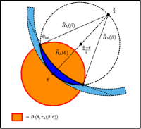
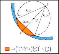
Figure 2: Our new GAP SAFE sphere and dome (in orange). The dual optimal solution $\hat{\theta}^{({\lambda})}$ must lie in the dark blue region; $\beta$ is any point in $\mathbb{R}^{p}$, and $\theta$ is any point in the dual feasible set $\Delta_{X}$. Remark that the GAP SAFE dome is included in the GAP SAFE sphere, and that it is the convex hull of the dark blue region.

3 New contributions on safe rules

3.1 Support discovery in finite time

Let us first introduce the notions of converging safe regions and converging safe tests.

Definition 1.

Let $(\mathcal{C}_{k})_{k\in\mathbb{N}}$ be a sequence of closed convex sets in $\mathbb{R}^{n}$ containing $\hat{\theta}^{({\lambda})}$. It is a converging sequence of safe regions for the Lasso with parameter $\lambda$ if the diameters of the sets converge to zero. The associated safe screening rules are referred to as converging safe tests.

Not only converging safe regions are crucial to speed up computation, but they are also helpful to reach exact active set identification in a finite number of steps. More precisely, we prove that one recovers the equicorrelation set of the Lasso (cf. Remark 2) in finite time with any converging strategy: after a finite number of steps, the equicorrelation set $\mathcal{E}_{\lambda}$ is exactly identified. Such a property is sometimes referred to as finite identification of the support (Liang et al., 2014). This is summarized in the following.

Theorem 1.

Let $(\mathcal{C}_{k})_{k\in\mathbb{N}}$ be a sequence of converging safe regions. The estimated support provided by $\mathcal{C}_{k}$, $A^{(\lambda)}(\mathcal{C}_{k})=\{j\in[p]:\max_{\theta\in\mathcal{C}_{k}}|\theta^{\top}x_{j}|\geq 1\}$, satisfies $\lim_{k\to\infty}A^{(\lambda)}(\mathcal{C}_{k})=\mathcal{E}_{\lambda}$, and there exists $k_{0}\in\mathbb{N}$ such that $\forall k\geq k_{0}$ one gets $A^{(\lambda)}(\mathcal{C}_{k})=\mathcal{E}_{\lambda}$.

Proof.

The main idea of the proof is to use that $\lim_{k\to\infty}\mathcal{C}_{k}=\{\hat{\theta}^{({\lambda})}\}$, $\lim_{k\to\infty}\mu_{\mathcal{C}_{k}}(x)=\mu_{\{\hat{\theta}^{({\lambda})}\}}(x)=|x^{\top}\hat{\theta}^{({\lambda})}|$ and that the set $A^{(\lambda)}(\mathcal{C}_{k})$ is discrete. Details are delayed to the Appendix. ∎

Remark 5.

A more general result is proved for a specific algorithm (Forward-Backward) in Liang et al. (2014). Interestingly, our scheme is independent of the algorithm considered (e.g., Forward-Backward (Beck & Teboulle, 2009), Primal Dual (Chambolle & Pock, 2011), coordinate-descent (Tseng, 2001; Friedman et al., 2007)) and relies only on the convergence of a sequence of safe regions.

3.2 GAP SAFE regions: leveraging the duality gap

In this section, we provide new dynamic safe rules built on converging safe regions.

Theorem 2.

Let us take any $(\beta,\theta)\in\mathbb{R}^{p}\times\Delta_{X}$. Denote $\widehat{R}_{\lambda}(\beta):=\frac{1}{\lambda}\big{(}\left\lVert y\right\rVert^{2}-\left\lVert X\beta-y\right\rVert^{2}-2\lambda\left\lVert\beta\right\rVert_{1}\big{)}_{+}^{1/2},\widecheck{R}_{\lambda}(\theta):=\left\lVert\theta-y/\lambda\right\rVert,\hat{\theta}^{({\lambda})}$ the dual optimal Lasso solution and ${\tilde{r}}_{\lambda}(\beta,\theta):=\sqrt{\widecheck{R}_{\lambda}(\theta)^{2}-\widehat{R}_{\lambda}(\beta)^{2}}$, then

$$\hat{\theta}^{({\lambda})}\in B\Big{(}\theta,{\tilde{r}}_{\lambda}(\beta,\theta)\Big{)}.$$ (15)

Proof.

The construction of the ball $B(\theta,{\tilde{r}}_{\lambda}(\beta,\theta))$ is based on the weak duality theorem (cf. (Rockafellar & Wets, 1998) for a reminder on weak and strong duality). Fix $\theta\in\Delta_{X}$ and $\beta\in\mathbb{R}^{p}$, then it holds that

$$\frac{1}{2}\left\lVert y\right\rVert^{2}-\frac{\lambda^{2}}{2}\left\lVert\theta-\frac{y}{\lambda}\right\rVert^{2}\leq\frac{1}{2}\left\lVert X\beta-y\right\rVert^{2}+\lambda\left\lVert\beta\right\rVert_{1}.$$

Hence,

$$\left\lVert\theta-\frac{y}{\lambda}\right\rVert\geq\!\frac{\sqrt{\left(\left\lVert y\right\rVert^{2}-\left\lVert X\beta-y\right\rVert^{2}-2\lambda\left\lVert\beta\right\rVert_{1}\right)_{+}}}{\lambda}.$$ (16)

In particular, this provides $\|\hat{\theta}^{({\lambda})}-y/\lambda\|\geq\widehat{R}_{\lambda}(\beta)$. Combining (12) and (16), asserts that $\hat{\theta}^{({\lambda})}$ belongs to the annulus $A(y/\lambda,\widecheck{R}_{\lambda}(\theta),\widehat{R}_{\lambda}(\beta)):=\{z\in\mathbb{R}^{n}:\widehat{R}_{\lambda}(\beta)\leq\|z-y/\lambda\|\leq\widecheck{R}_{\lambda}(\theta)\}$ (the light blue zone in Figure 2).

Remind that the dual feasible set $\Delta_{X}$ is convex, hence $\Delta_{X}\cap B(y/\lambda,\widecheck{R}_{\lambda}(\theta))$ is also convex. Thanks to (16), $\Delta_{X}\cap B(y/\lambda,\widecheck{R}_{\lambda}(\theta))=\Delta_{X}\cap A(y/\lambda,\widecheck{R}_{\lambda}(\theta),\widehat{R}_{\lambda}(\beta))$, and then $\Delta_{X}\cap A(y/\lambda,\widecheck{R}_{\lambda}(\theta),\widehat{R}_{\lambda}(\beta))$ is convex too. Hence, $\hat{\theta}^{({\lambda})}$ is inside the annulus $A(y/\lambda,\widecheck{R}_{\lambda}(\theta),\widehat{R}_{\lambda}(\beta))$ and so is $[\theta,\hat{\theta}^{({\lambda})}]\subseteq A(y/\lambda,\widecheck{R}_{\lambda}(\theta),\widehat{R}_{\lambda}(\beta))$ by convexity (see Figure 2,(a) and Figure 2,(b)). Moreover, $\hat{\theta}^{({\lambda})}$ is the point of $[\theta,\hat{\theta}^{({\lambda})}]$ which is closest to $y/\lambda$. The farthest where $\hat{\theta}^{({\lambda})}$ can be according to this information would be if $[\theta,\hat{\theta}^{({\lambda})}]$ were tangent to the inner ball $B(y/\lambda,\widehat{R}_{\lambda}(\beta))$ and $\|\hat{\theta}^{({\lambda})}-y/\lambda\|=\widehat{R}_{\lambda}(\beta)$. Let us denote $\theta_{\rm{int}}$ such a point. The tangency property reads $\left\lVert\theta_{\rm{int}}-y/\lambda\right\rVert=\widehat{R}_{\lambda}(\beta)$ and $(\theta-\theta_{\rm{int}})^{\top}(y/\lambda-\theta_{\rm{int}})=0$. Hence, with the later and the definition of $\widecheck{R}_{\lambda}(\theta)$, $\left\lVert\theta-y/\lambda\right\rVert^{2}=\left\lVert\theta-\theta_{\rm{int}}\right\rVert^{2}+\left\lVert\theta_{\rm{int}}-y/\lambda\right\rVert^{2}$and $\left\lVert\theta-\theta_{\rm{int}}\right\rVert^{2}=\widecheck{R}_{\lambda}(\theta)^{2}-\widehat{R}_{\lambda}(\beta)^{2}$.

Since by construction $\hat{\theta}^{({\lambda})}$ cannot be further away from $\theta$ than $\theta_{\rm{int}}$ (again, insights can be gleaned from Figure 2), we conclude that $\hat{\theta}^{({\lambda})}\in B\big{(}\theta,(\widecheck{R}_{\lambda}(\theta)^{2}-\widehat{R}_{\lambda}(\beta)^{2})^{1/2}\big{)}$. ∎

Remark 6.

Choosing $\beta=0$ and $\theta=y/\lambda_{\max}$, then one recovers the static safe rule given in Example 1.

With the definition of the primal (resp. dual) objective for $P_{\lambda}(\beta)$, (resp. $D_{\lambda}(\theta)$), the duality gap reads as $G_{\lambda}(\beta,\theta)=P_{\lambda}(\beta)-D_{\lambda}\left(\theta\right)$. Remind that if $G_{\lambda}(\beta,\theta)\leq\epsilon$, then one has $P_{\lambda}(\beta)-P_{\lambda}(\hat{\beta}^{({\lambda})})\leq\epsilon$, which is a standard stopping criterion for Lasso solvers. The next proposition establishes a connection between the radius ${r}_{\lambda}(\beta,\theta)$ and the duality gap $G_{\lambda}(\beta,\theta)$.

Proposition 1.

For any $(\beta,\theta)\in\mathbb{R}^{p}\times\Delta_{X}$, the following holds

$${\tilde{r}}_{\lambda}(\beta,\theta)^{2}\leq{r}_{\lambda}(\beta,\theta)^{2}:=\frac{2}{\lambda^{2}}G_{\lambda}(\beta,\theta).$$ (17)

Proof.

Use the fact that $\widecheck{R}_{\lambda}(\theta)^{2}=\left\lVert\theta-y/\lambda\right\rVert^{2}$ and $\widehat{R}_{\lambda}(\beta)^{2}\geq(\left\lVert y\right\rVert^{2}-\left\lVert X\beta-y\right\rVert^{2}-2\lambda\left\lVert\beta\right\rVert_{1})/\lambda^{2}$. ∎

If we could choose the “oracle” $\theta=\hat{\theta}^{({\lambda})}$ and $\beta=\hat{\beta}^{({\lambda})}$ in (15) then we would obtain a zero radius. Since those quantities are unknown, we rather pick dynamically the current available estimates given by an optimization algorithm: $\beta=\beta_{k}$ and $\theta=\theta_{k}$ as in Eq. (11). Introducing GAP SAFE spheres and domes as below, Proposition 2 ensures that they are converging safe regions.

GAP SAFE sphere:

$$\mathcal{C}_{k}=B\left(\theta_{k},{r}_{\lambda}(\beta,\theta)\right).$$ (18)

GAP SAFE dome:

$$\mathcal{C}_{k}=D\!\!\left(\frac{\frac{y}{\lambda}+\theta_{k}}{2},\frac{\widecheck{R}_{\lambda}(\theta_{k})}{2},2\left(\!\frac{\widehat{R}_{\lambda}(\beta_{k})}{\widecheck{R}_{\lambda}(\theta_{k})}\right)^{2}\!\!\!-1,\frac{\theta_{k}-\frac{y}{\lambda}}{\|\theta_{k}-\frac{y}{\lambda}\|}\right).$$ (19)

Proposition 2.

For any converging primal sequence $(\beta_{k})_{k\in\mathbb{N}}$, and dual sequence $(\theta_{k})_{k\in\mathbb{N}}$ defined as in Eq. (11), then the GAP SAFE sphere and the GAP SAFE dome are converging safe regions.

Proof.

For the GAP SAFE sphere the result follows from strong duality, Remark 4 and Proposition 1 yield $\lim_{k\to\infty}{r}_{\lambda}(\beta_{k},\theta_{k})=0$, since $\lim_{k\to\infty}\theta_{k}=\hat{\theta}^{({\lambda})}$ and $\lim_{k\to\infty}\beta_{k}=\hat{\beta}^{({\lambda})}$. For the GAP SAFE dome, one can check that it is included in the GAP SAFE sphere, therefore inherits the convergence (see also Figure 2,(c) and (d)). ∎

Remark 7.

The radius ${r}_{\lambda}(\beta_{k},\theta_{k})$ can be compared with the radius considered for the Dynamic Safe rule and Dynamic ST3 (Bonnefoy et al., 2014a) respectively: $\widecheck{R}_{\lambda}(\theta_{k})=\|\theta_{k}-y/\lambda\|^{2}$ and $(\widecheck{R}_{\lambda}(\theta_{k})^{2}-\delta^{2})^{1/2}$, where $\delta=(\lambda_{\max}/\lambda-1)/\left\lVert x_{j^{\star}}\right\rVert$. We have proved that $\lim_{k\to\infty}{r}_{\lambda}(\beta_{k},\theta_{k})=0$, but a weaker property is satisfied by the two other radius: $\lim_{k\to\infty}\widecheck{R}_{\lambda}(\theta_{k})=\widecheck{R}_{\lambda}(\hat{\theta}^{({\lambda})})=\|\widecheck{R}_{\lambda}(\hat{\theta}^{({\lambda})})-y/\lambda\|^{2}$ and $\lim_{k\to\infty}(\widecheck{R}_{\lambda}(\theta_{k})^{2}-\delta^{2})^{1/2}=(\widecheck{R}_{\lambda}(\hat{\theta}^{({\lambda})})^{2}-\delta^{2})^{1/2}>0$.

3.3 GAP SAFE rules : sequential for free

As a byproduct, our dynamic screening tests provide a warm start strategy for the safe regions, making our GAP SAFE rules inherently sequential. The next proposition shows their efficiency when attacking a new tuning parameter, after having solved the Lasso for a previous $\lambda$, even only approximately. Handling approximate solutions is a critical issue to produce safe sequential strategies: without taking into account the approximation error, the screening might disregard relevant variables, especially the one near the safe regions boundaries. Except for $\lambda_{\max}$, it is unrealistic to assume that one can dispose of exact solutions.

Consider $\lambda_{0}=\lambda_{\max}$ and a non-increasing sequence of $T-1$ tuning parameters $(\lambda_{t})_{t\in[T-1]}$ in $(0,\lambda_{\max})$. In practice, we choose the common grid (Bühlmann & van de Geer, 2011)[2.12.1]): $\lambda_{t}=\lambda_{0}10^{-\delta t/(T-1)}$ (for instance in Figure 3, we considered $\delta=3$). The next result controls how the duality gap, or equivalently, the diameter of our GAP SAFE regions, evolves from $\lambda_{t-1}$ to $\lambda_{t}$.

Proposition 3.

Suppose that $t\geq 1$ and $(\beta,\theta)\in\mathbb{R}^{p}\times\Delta_{X}$. Reminding ${r}_{\lambda_{t}}^{2}(\beta,\theta)=2G_{\lambda_{t}}(\beta,\theta)/\lambda_{t}^{2}$, the following holds

$${r}_{\lambda_{t}}^{2}(\beta,\theta) =\left(\frac{\lambda_{t-1}}{\lambda_{t}}\right){r}_{\lambda_{t-1}}^{2}(\beta,\theta)$$ (20)

$$+(1-\frac{\lambda_{t}}{\lambda_{t-1}})\left\lVert\frac{X\beta-y}{\lambda_{t}}\right\rVert^{2}-(\frac{\lambda_{t-1}}{\lambda_{t}}-1)\left\lVert\theta\right\rVert^{2}.$$

Proof.

Details are given in the Appendix. ∎

This proposition motivates to screen sequentially as follows: having $(\beta,\theta)\in\mathbb{R}^{p}\times\Delta_{X}$ such that $G_{\lambda_{t-1}}(\beta,\theta)\leq\epsilon$, then, we can screen using the GAP SAFE sphere with center $\theta$ and radius ${r}_{\lambda}(\beta,\theta)$. The adaptation to the GAP SAFE dome is straightforward and consists in replacing $\theta_{k},\beta_{k},\lambda$ by $\theta,\beta,\lambda_{t}$ in the GAP SAFE dome definition.

Remark 8.

The basic sphere test of (Wang et al., 2013) requires the exact dual solution $\theta=\hat{\theta}^{({\lambda_{t-1}})}$ for center, and has radius $|1/\lambda_{t}-1/\lambda_{t-1}|\left\lVert y\right\rVert$, which is strictly larger than ours. Indeed, if one has access to dual and primal optimal solutions at $\lambda_{t-1}$, i.e., $(\theta,\beta)=(\hat{\theta}^{({\lambda_{t-1}})},\hat{\beta}^{({\lambda_{t-1}})})$, then ${r}_{\lambda_{t-1}}^{2}(\beta,\theta)=0$, $\theta=(y-X\beta)/\lambda_{t-1}$ and

$${r}_{\lambda_{t}}^{2}(\beta,\theta) =\left(\frac{\lambda_{t-1}^{2}}{\lambda_{t}^{2}}(1-\frac{\lambda_{t}}{\lambda_{t-1}})-(\frac{\lambda_{t-1}}{\lambda_{t}}-1)\right)\left\lVert\theta\right\rVert^{2},$$

$$\leq\left(\frac{1}{\lambda_{t}}-\frac{1}{\lambda_{t-1}}\right)^{2}\left\lVert y\right\rVert^{2},$$

since $\|\theta\|\leq\|y\|/\lambda_{t-1}$ for $\theta=\hat{\theta}^{({\lambda_{t-1}})}$.

Note that contrarily to former sequential rules (Wang et al., 2013), our introduced GAP SAFE rules still work when one has only access to approximations of $\hat{\theta}^{({\lambda_{t-1}})}$.

4 Experiments

4.1 Coordinate Descent

Screening procedures can be used with any optimization algorithm. We chose coordinate descent because it is well suited for machine learning tasks, especially with sparse and/or unstructured design matrix $X$. Coordinate descent requires to extract efficiently columns of $X$ which is typically not easy in signal processing applications where $X$ is commonly an implicit operator (e.g. Fourier or wavelets).

Algorithm 1 Coordinate descent with GAP SAFE rules

0:  $X,y,\epsilon,K,f,(\lambda_{t})_{t\in[T-1]}$

  Initialization:

   $\lambda_{0}=\lambda_{\max}$

   $\beta^{\lambda_{0}}=0$

  for $t\in[T-1]$ do

     $\beta\leftarrow\beta^{\lambda_{t-1}}$ (previous $\epsilon$-solution)

     for $k\in[K]$ do

        if $k\mod f=1$ then

           Compute $\theta$ and $\mathcal{C}$ thanks to (11) and (18) or (19)

           Get $A^{\lambda_{t}}(\mathcal{C})=\{j\in[p]:\mu_{\mathcal{C}}(x_{j})\geq 1\}$ as in (7)

           if $G_{\lambda_{t}}(\beta,\theta)\leq\epsilon$ then

              $\beta^{\lambda_{t}}\leftarrow\beta$

              break

        for $j\in A^{\lambda_{t}}(\mathcal{C})$ do

           $\beta_{j}\leftarrow\mathrm{ST}\big{(}\frac{\lambda_{t}}{\left\lVert x_{j}\right\rVert^{2}},\beta_{j}-\frac{x_{j}^{\top}(X\beta-y)}{\left\lVert x_{j}\right\rVert^{2}}\big{)}$

           # $\mathrm{ST}(u,x)=\operatorname{sign}(x)\left(|x|-u\right)_{+}$ (soft-threshold)

  $(\beta^{\lambda_{t}})_{t\in[T-1]}$

We implemented the screening rules of Table 1 based on the coordinate descent in Scikit-learn (Pedregosa et al., 2011). This code is written in Python and Cython to generate low level C code, offering high performance. A low level language is necessary for this algorithm to scale. Two implementations were written to work efficiently with both dense data stored as Fortran ordered arrays and sparse data stored in the compressed sparse column (CSC) format. Our pseudo-code is presented in Algorithm 1. In practice, we perform the dynamic screening tests every $f=10$ passes through the entire (active) variables. Iterations are stopped when the duality gap is smaller than the target accuracy.

The naive computation of $\theta_{k}$ in (11) involves the computation of $\left\lVert X^{\top}\rho_{k}\right\rVert_{\infty}$ ($\rho_{k}$ being the current residual), which costs $\mathcal{O}(np)$ operations. This can be avoided as one knows when using a safe rule that the index achieving the maximum for this norm is in $A^{\lambda_{t}}(\mathcal{C})$. Indeed, by construction $\mathop{\mathrm{arg\,max}}_{j\in A^{\lambda_{t}}(\mathcal{C})}|x_{j}^{\top}\theta_{k}|=\mathop{\mathrm{arg\,max}}_{j\in[p]}|x_{j}^{\top}\theta_{k}|=\mathop{\mathrm{arg\,max}}_{j\in[p]}|x_{j}^{\top}\rho_{k}|$. In practice the evaluation of the dual gap is therefore not a $\mathcal{O}(np)$ but $\mathcal{O}(nq)$ where $q$ is the size of $A^{\lambda_{t}}(\mathcal{C})$. In other words, using screening also speeds up the evaluation of the stopping criterion.

We did not compare our method against the strong rules of Tibshirani et al. (2012) because they are not safe and therefore need complex post-processing with parameters to tune. Also we did not compare against the sequential rule of Wang et al. (2013) (e.g., EDDP) because it requires the exact dual optimal solution of the previous Lasso problem, which is not available in practice and can prevent the solver from actually converging: this is a phenomenon we always observed on our experiments.

4.2 Number of screened variables

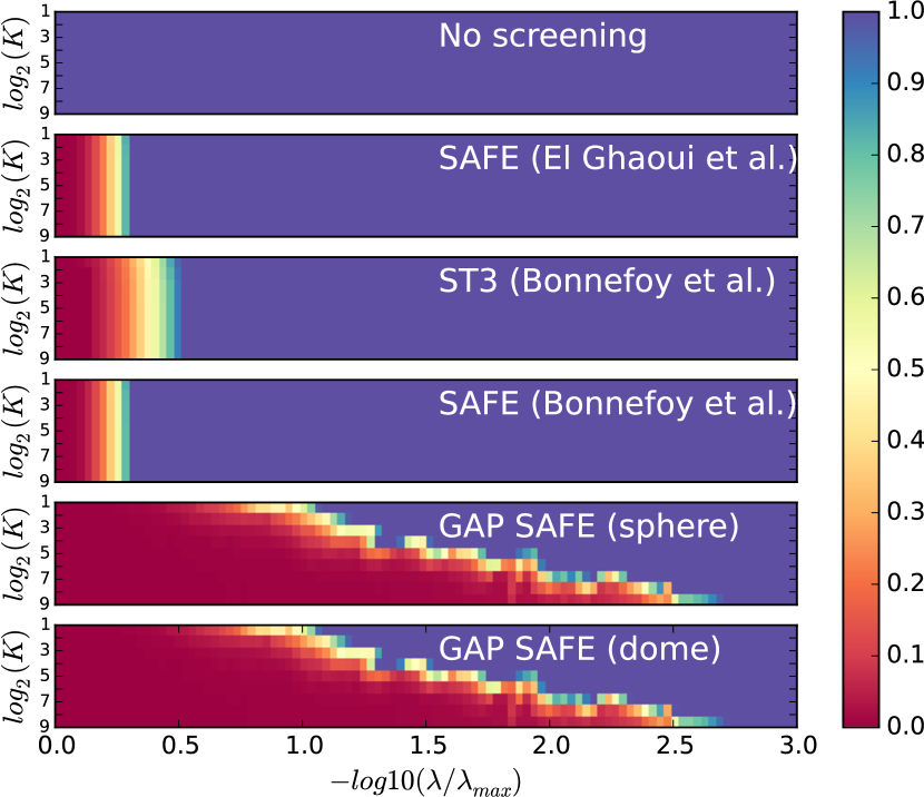
Figure 3: Proportion of active variables as a function of $\lambda$ and the number of iterations $K$ on the Leukemia dataset. Better strategies have longer range of $\lambda$ with (red) small active sets.

Figure 3 presents the proportion of variables screened by several safe rules on the standard Leukemia dataset. The screening proportion is presented as a function of the number of iterations $K$. As the SAFE screening rule of El Ghaoui et al. (2012) is sequential but not dynamic, for a given $\lambda$ the proportion of screened variables does not depend on $K$. The rules of Bonnefoy et al. (2014a) are more efficient on this dataset but they do not benefit much from the dynamic framework. Our proposed GAP SAFE tests screen much more variables, especially when the tuning parameter $\lambda$ gets small, which is particularly relevant in practice. Moreover, even for very small $\lambda$’s (notice the logarithmic scale) where no variable is screened at the beginning of the optimization procedure, the GAP SAFE rules manage to screen more variables, especially when $K$ increases. Finally, the figure demonstrates that the GAP SAFE dome test only brings marginal improvement over the sphere.

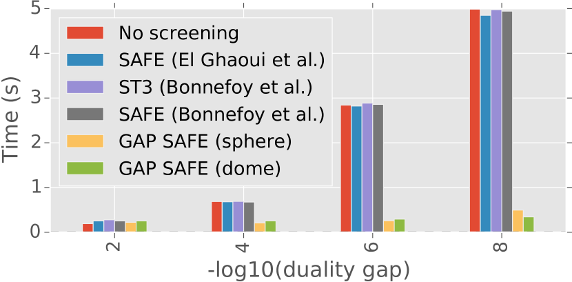
Figure 4: Time to reach convergence using various screening rules on the Leukemia dataset (dense data: $n=72,p=7129$).

4.3 Gains in the computation of Lasso paths

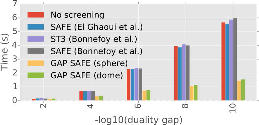
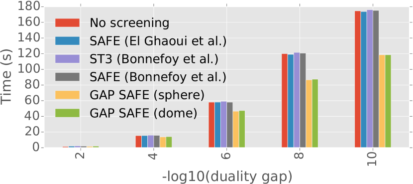
The main interest of variable screening is to reduce computation costs. Indeed, the time to compute the screening itself should not be larger than the gains it provides. Hence, we compared the time needed to compute Lasso paths to prescribed accuracy for different safe rules. Figures 4, 5 and 6 illustrate results on three datasets. Figure 4 presents results on the dense, small scale, Leukemia dataset. Figure 5 presents results on a medium scale sparse dataset obtained with bag of words features extracted from the 20newsgroup dataset (comp.graphics vs. talk.religion.misc with TF-IDF removing English stop words and words occurring only once or more than 95% of the time). Text feature extraction was done using Scikit-Learn. Figure 6 focuses on the large scale sparse RCV1 (Reuters Corpus Volume 1) dataset, cf. (Schmidt et al., 2013).

In all cases, Lasso paths are computed as required to estimate optimal regularization parameters in practice (when using cross-validation one path is computed for each fold). For each Lasso path, solutions are obtained for $T=100$ values of $\lambda$’s, as detailed in Section 3.3. Remark that the grid used is the default one in both Scikit-Learn and the glmnet R package. With our proposed GAP SAFE screening we obtain on all datasets substantial gains in computational time. We can already get an up to 3x speedup when we require a duality gap smaller than $10^{-4}$. The interest of the screening is even clearer for higher accuracies: GAP SAFE sphere is 11x faster than its competitors on the Leukemia dataset, at accuracy $10^{-8}$. One can observe that with the parameter grid used here, the larger is $p$ compared to $n$, the higher is the gain in computation time.

In our experiments, the other safe screening rules did not show much speed-up. As one can see on Figure 3, those screening rules keep all the active variables for a wide range of $\lambda$’s. The algorithm is thus faster for large $\lambda$’s but slower afterwards, since we still compute the screening tests. Even if one can avoid some of these useless computations thanks to formulas like (14) or (10), the corresponding speed-up would not be significant.

Figure 5: Time to reach convergence using various screening rules on bag of words from the 20newsgroup dataset (sparse data: with $n=961,p=10094$).

Figure 6: Computation time to reach convergence using different screening strategies on the RCV1 (Reuters Corpus Volume 1) dataset (sparse data with $n=20242$ and $p=47236$).

5 Conclusion

We have presented new results on safe rules for accelerating algorithms solving the Lasso problem (see Appendix for extension to the Elastic Net). First, we have introduced the framework of converging safe rules, a key concept independent of the implementation chosen. Our second contribution was to leverage duality gap computations to create two safer rules satisfying the aforementioned convergence properties. Finally, we demonstrated the important practical benefits of those new rules by applying them to standard dense and sparse datasets using a coordinate descent solver. Future works will extend our framework to generalized linear model and group-Lasso.

Appendix A Supplementary materials

We provided in this Appendix some more details on the theoretical results given in the main part.

A.1 Dome test

Let us consider the case where the safe region $\mathcal{C}$ is the dome $\mathcal{D}(c,r,\alpha,w)$, with parameters: center $c$, radius $r$, relative distance ratio $\alpha$ and unit normal vector $w$.

The computation of the dome test formula proceeds as follows:

$$\sigma_{\mathcal{C}}(x_{j})=\begin{cases}c^{\top}x_{j}+r\|x_{j}\|&\text{ if }w^{\top}x_{j}<-\alpha\|x_{j}\|,\\ c^{\top}x_{j}-r\alpha w^{\top}x_{j}+r\sqrt{(\|x_{j}\|^{2}-|w^{\top}x_{j}|^{2})(1-\alpha^{2})}&\text{ otherwise. }\end{cases}$$ (21)

and so

$$\sigma_{\mathcal{C}}(-x_{j})=\begin{cases}-c^{\top}x_{j}+r\|x_{j}\|&\text{ if }-w^{\top}x_{j}<-\alpha\|x_{j}\|,\\ -c^{\top}x_{j}+r\alpha w^{\top}x_{j}+r\sqrt{(\|x_{j}\|^{2}-|w^{\top}x_{j}|^{2})(1-\alpha^{2})}&\text{ otherwise. }\end{cases}$$ (22)

With the previous display we can now compute $\mu_{\mathcal{C}}(x_{j}):=\max(\sigma_{\mathcal{C}}(x_{j}),\sigma_{\mathcal{C}}(-x_{j}))$. Thanks to the Eq. (6), we express our dome test as:

$$\text{ If }\,M_{\min}<c^{\top}x_{j}<M_{\max},\,\text{ then }\,\hat{\beta}^{({\lambda})}_{j}=0.$$ (23)

Using the former notation:

$$M_{\max}=\begin{cases}1-r\|x_{j}\|&\text{ if }w^{\top}x_{j}<-\alpha\|x_{j}\|,\\ 1+r\alpha w^{\top}x_{j}-r\sqrt{(\|x_{j}\|^{2}-|w^{\top}x_{j}|^{2})(1-\alpha^{2})}&\text{ otherwise. }\end{cases}$$ (24)

$$M_{\min}=\begin{cases}-1+r\|x_{j}\|&\text{ if }-w^{\top}x_{j}<-\alpha\|x_{j}\|,\\ -1+r\alpha w^{\top}x_{j}+r\sqrt{(\|x_{j}\|^{2}-|w^{\top}x_{j}|^{2})(1-\alpha^{2})}&\text{ otherwise. }\end{cases}$$ (25)

Let us introduce the following dome parameters, for any $\theta\in\Delta_{X}$:

• Center: $c=(y/\lambda+\theta)/2$.

• Radius: $r=\widecheck{R}_{\lambda}(\theta)/2$.

• Ratio: $\alpha=-1+2\widehat{R}_{\lambda}(\theta)^{2}/\widecheck{R}_{\lambda}(\theta)^{2}$.

• Normal vector: $w=(y/\lambda-\theta)/\widecheck{R}_{\lambda}(\theta)$.

Reminding that the support function of a set is the same as the support function of its closed convex hull (Hiriart-Urruty & Lemaréchal, 1993)[Proposition V.2.2.1] means that we only need to optimize over the dome introduced. Therefore, one cannot improve our previous result by optimizing the problem on the intersection of the ball of radius $\widecheck{R}_{\lambda}(\theta)$ and the complement of the ball of radius $\widehat{R}_{\lambda}(\beta)$ (i.e., the blue region in Figure 2).

A.2 Proof of Theorem 1

Proof.

Define $\max_{j\notin\mathcal{E}_{\lambda}}|x_{j}^{\top}\hat{\theta}^{({\lambda})}|=t<1$. Fix $\epsilon>0$ such that $\epsilon<(1-t)/(\max_{j\notin\mathcal{E}_{\lambda}}\|x_{j}\|)$. As $\mathcal{C}_{k}$ is a converging sequence containing $\hat{\theta}^{({\lambda})}$, its diameter is converging to zero, and there exists $k_{0}\in\mathbb{N}$ such that $\forall k\geq k_{0},\forall\theta\in\mathcal{C}_{k},\|\theta-\hat{\theta}^{({\lambda})}\|\leq\epsilon$. Hence, for any $j\notin\mathcal{E}_{\lambda}$ and any $\theta\in\mathcal{C}_{k}$, $|x_{j}^{\top}(\theta-\hat{\theta}^{({\lambda})})|\leq(\max_{j\notin\mathcal{E}_{\lambda}}\|x_{j}\|)\|\theta-\hat{\theta}^{({\lambda})}\|\leq(\max_{j\notin\mathcal{E}_{\lambda}}\|x_{j}\|)\epsilon$. Using the triangle inequality, one gets

$$|x_{j}^{\top}\theta|\leq (\max_{j\notin\mathcal{E}_{\lambda}}\|x_{j}\|)\epsilon+\max_{j\notin\mathcal{E}_{\lambda}}|x_{j}^{\top}\hat{\theta}^{({\lambda})}|$$

$$\leq (\max_{j\notin\mathcal{E}_{\lambda}}\|x_{j}\|)\epsilon+t<1,$$

provided that $\epsilon<(1-t)/(\max_{j\notin\mathcal{E}_{\lambda}}\|x_{j}\|)$. Thus, for any $k\geq k_{0},\mathcal{E}_{\lambda}^{c}\subset Z^{(\lambda)}(\mathcal{C}_{k})=A^{(\lambda)}(\mathcal{C}_{k})^{c}$ and $A^{(\lambda)}(\mathcal{C}_{k})\subset\mathcal{E}_{\lambda}$.

For the reverse inclusion take $j\in\mathcal{E}_{\lambda}$, i.e., $|x_{j}^{\top}\hat{\theta}^{({\lambda})}|=1$. Since for all $k\in\mathbb{N},\hat{\theta}^{({\lambda})}\in\mathcal{C}_{k}$, then $j\in A^{(\lambda)}(\mathcal{C}_{k})=\{j\in[p]:\max_{\theta\in\mathcal{C}_{k}}|x_{j}^{\top}\theta|\geq 1\}$ and the result holds.

∎

A.3 Proof of Proposition 3

We detail here the proof of Proposition 3.

Proof.

We first use the fact that

$$G_{\lambda_{t-1}}(\beta,\theta)=\frac{1}{2}\left\lVert X\beta-y\right\rVert^{2}_{2}+\lambda_{t-1}\left\lVert\beta\right\rVert_{1}-\frac{1}{2}\left\lVert y\right\rVert_{2}^{2}+\frac{\lambda_{t-1}^{2}}{2}\left\lVert\theta-\frac{y}{\lambda_{t-1}}\right\rVert^{2}_{2},$$

to obtain

$$\left\lVert\beta\right\rVert_{1}=\frac{1}{\lambda_{t-1}}\Big{(}\frac{1}{2}\left\lVert y\right\rVert_{2}^{2}-\left\lVert X\beta-y\right\rVert^{2}_{2}-\frac{\lambda_{t-1}^{2}}{2}\left\lVert\theta-\frac{y}{\lambda_{t-1}}\right\rVert^{2}_{2}+G_{\lambda_{t-1}}(\beta,\theta)\Big{)}.$$

Then,

$$G_{\lambda_{t}}(\beta, \theta)=\frac{1}{2}\left\lVert X\beta-y\right\rVert^{2}_{2}+\frac{\lambda_{t}}{\lambda_{t-1}}\Big{(}\frac{1}{2}\left\lVert y\right\rVert_{2}^{2}-\frac{1}{2}\left\lVert X\beta-y\right\rVert^{2}_{2}-\frac{\lambda_{t-1}^{2}}{2}\left\lVert\theta-\frac{y}{\lambda_{t-1}}\right\rVert^{2}_{2}+G_{\lambda_{t-1}}(\beta,\theta)\Big{)}$$

$$\qquad\qquad-\frac{1}{2}\left\lVert y\right\rVert^{2}_{2}+\frac{\lambda_{t}^{2}}{2}\left\lVert\theta-\frac{y}{\lambda_{t}}\right\rVert^{2}_{2}$$

$$= \frac{1}{2}(\frac{\lambda_{t}}{\lambda_{t-1}}-1)\left\lVert y\right\rVert_{2}^{2}+\frac{1}{2}(1-\frac{\lambda_{t}}{\lambda_{t-1}})\left\lVert X\beta-y\right\rVert^{2}_{2}+\frac{\lambda_{t}}{\lambda_{t-1}}G_{\lambda_{t-1}}(\beta,\theta)+\frac{1}{2}\big{(}\left\lVert\lambda_{t}\theta-y\right\rVert^{2}_{2}-\frac{\lambda_{t}}{\lambda_{t-1}}\left\lVert\lambda_{t-1}\theta-y\right\rVert^{2}_{2}\big{)}$$

$$= \frac{1}{2}(\frac{\lambda_{t}}{\lambda_{t-1}}-1)\left\lVert y\right\rVert_{2}^{2}+\frac{1}{2}(1-\frac{\lambda_{t}}{\lambda_{t-1}})\left\lVert X\beta-y\right\rVert^{2}_{2}+\frac{\lambda_{t}}{\lambda_{t-1}}G_{\lambda_{t-1}}(\beta,\theta)$$

$$\qquad\qquad+\frac{1}{2}\Big{(}\left\lVert\lambda_{t}\theta-y\right\rVert^{2}_{2}-\frac{\lambda_{t}}{\lambda_{t-1}}\big{(}\left\lVert\lambda_{t}\theta-y\right\rVert^{2}_{2}+\left\lVert(\lambda_{t-1}-\lambda_{t})\theta\right\rVert_{2}^{2}+2(\lambda_{t}\theta-y)^{\top}(\lambda_{t-1}-\lambda_{t})\theta\big{)}\Big{)}.$$

We deal with the dot product as

$$2\lambda_{t}(\lambda_{t-1}-\lambda_{t})(\theta-\frac{y}{\lambda_{t}})^{\top}\theta=\lambda_{t}(\lambda_{t-1}-\lambda_{t})\big{(}\left\lVert\theta\right\rVert^{2}_{2}+\left\lVert\theta-\frac{y}{\lambda_{t}}\right\rVert^{2}_{2}-\left\lVert\frac{y}{\lambda_{t}}\right\rVert^{2}_{2}\big{)}.$$

Hence,

$$G_{\lambda_{t}}(\beta,\theta)= \frac{1}{2}(\frac{\lambda_{t}}{\lambda_{t-1}}-1+\frac{1}{\lambda_{t-1}}(\lambda_{t-1}-\lambda_{t}))\left\lVert y\right\rVert_{2}^{2}+\frac{1}{2}(1-\frac{\lambda_{t}}{\lambda_{t-1}})\left\lVert X\beta-y\right\rVert^{2}_{2}$$

$$-\frac{\lambda_{t}}{2}(\lambda_{t-1}-\lambda_{t}))\left\lVert\theta\right\rVert^{2}_{2}+\frac{1}{2}(1-\frac{\lambda_{t}}{\lambda_{t-1}}-\frac{1}{\lambda_{t-1}}(\lambda_{t-1}-\lambda_{t}))\left\lVert\lambda_{t}\theta-y\right\rVert^{2}_{2}+\frac{\lambda_{t}}{\lambda_{t-1}}G_{\lambda_{t-1}}(\beta,\theta)$$

$$= \frac{1}{2}\left(1-\frac{\lambda_{t}}{\lambda_{t-1}}\right)\left\lVert X\beta-y\right\rVert^{2}_{2}-\frac{\lambda_{t}}{2}(\lambda_{t-1}-\lambda_{t}))\|\theta\|^{2}+\frac{\lambda_{t}}{\lambda_{t-1}}G_{\lambda_{t-1}}(\beta,\theta).$$

We observe in the end that

$$\frac{2}{\lambda_{t}^{2}}G_{\lambda_{t}}(\beta,\theta)= \left(1-\frac{\lambda_{t}}{\lambda_{t-1}}\right)\left\lVert\frac{X\beta-y}{\lambda_{t}}\right\rVert^{2}_{2}-\left(\frac{\lambda_{t-1}}{\lambda_{t}}-1\right)\left\lVert\theta\right\rVert^{2}_{2}+\frac{2}{\lambda_{t-1}\lambda_{t}}G_{\lambda_{t-1}}(\beta,\theta).$$

∎

A.4 Elastic-Net

The previously proposed tests can be adapted straightforwardly to the Elastic-Net estimator (Zou & Hastie, 2005). We provide here some more details for the interested reader.

$$\min_{\beta\in\mathbb{R}^{p}}\frac{1}{2}\left\lVert X\beta-y\right\rVert_{2}^{2}+\lambda\alpha\left\lVert\beta\right\rVert_{1}+\frac{\lambda}{2}(1-\alpha)\left\lVert\beta\right\rVert_{2}^{2}.$$ (26)

One can reformulate this problem as a Lasso problem

$$\min_{\beta\in\mathbb{R}^{p}}\frac{1}{2}\left\lVert\tilde{X}\beta-\tilde{y}\right\rVert_{2}^{2}+\lambda\alpha\left\lVert\beta\right\rVert_{1},$$ (27)

where $\tilde{X}=\begin{pmatrix}X\\ \sqrt{(1-\alpha)\lambda}I_{p}\end{pmatrix}\in\mathbb{R}^{n+p,p}$ and $\tilde{y}=\begin{pmatrix}y\\ 0\end{pmatrix}\in\mathbb{R}^{n+p}.$ With this modification all the tests introduced for the Lasso can be adapted for the Elastic-Net.

References

• Bach (2008) Bach, F. Bolasso: model consistent Lasso estimation through the bootstrap. In ICML, 2008.
• Beck & Teboulle (2009) Beck, A. and Teboulle, M. A fast iterative shrinkage-thresholding algorithm for linear inverse problems. SIAM J. Imaging Sci., 2(1):183–202, 2009.
• Bickel et al. (2009) Bickel, P. J., Ritov, Y., and Tsybakov, A. B. Simultaneous analysis of Lasso and Dantzig selector. Ann. Statist., 37(4):1705–1732, 2009.
• Bonnefoy et al. (2014a) Bonnefoy, A., Emiya, V., Ralaivola, L., and Gribonval, R. A dynamic screening principle for the lasso. In EUSIPCO, 2014a.
• Bonnefoy et al. (2014b) Bonnefoy, A., Emiya, V., Ralaivola, L., and Gribonval, R. Dynamic Screening: Accelerating First-Order Algorithms for the Lasso and Group-Lasso. ArXiv e-prints, 2014b.
• Bühlmann & van de Geer (2011) Bühlmann, P. and van de Geer, S. Statistics for high-dimensional data. Springer Series in Statistics. Springer, Heidelberg, 2011. Methods, theory and applications.
• Candès et al. (2008) Candès, E. J., Wakin, M. B., and Boyd, S. P. Enhancing sparsity by reweighted l1subscript𝑙1l_{1} minimization. J. Fourier Anal. Applicat., 14(5-6):877–905, 2008.
• Chambolle & Pock (2011) Chambolle, A. and Pock, T. A first-order primal-dual algorithm for convex problems with applications to imaging. J. Math. Imaging Vis., 40(1):120–145, 2011.
• Chen et al. (1998) Chen, S. S., Donoho, D. L., and Saunders, M. A. Atomic decomposition by basis pursuit. SIAM J. Sci. Comput., 20(1):33–61 (electronic), 1998.
• Efron et al. (2004) Efron, B., Hastie, T., Johnstone, I. M., and Tibshirani, R. Least angle regression. Ann. Statist., 32(2):407–499, 2004. With discussion, and a rejoinder by the authors.
• El Ghaoui et al. (2012) El Ghaoui, L., Viallon, V., and Rabbani, T. Safe feature elimination in sparse supervised learning. J. Pacific Optim., 8(4):667–698, 2012.
• Fan & Li (2001) Fan, J. and Li, R. Variable selection via nonconcave penalized likelihood and its oracle properties. J. Amer. Statist. Assoc., 96(456):1348–1360, 2001.
• Fan & Lv (2008) Fan, J. and Lv, J. Sure independence screening for ultrahigh dimensional feature space. J. Roy. Statist. Soc. Ser. B, 70(5):849–911, 2008.
• Friedman et al. (2007) Friedman, J., Hastie, T., Höfling, H., and Tibshirani, R. Pathwise coordinate optimization. Ann. Appl. Stat., 1(2):302–332, 2007.
• Gramfort et al. (2012) Gramfort, A., Kowalski, M., and Hämäläinen, M. Mixed-norm estimates for the M/EEG inverse problem using accelerated gradient methods. Phys. Med. Biol., 57(7):1937–1961, 2012.
• Haury et al. (2012) Haury, A.-C., Mordelet, F., Vera-Licona, P., and Vert, J.-P. TIGRESS: Trustful Inference of Gene REgulation using Stability Selection. BMC systems biology, 6(1):145, 2012.
• Hiriart-Urruty & Lemaréchal (1993) Hiriart-Urruty, J.-B. and Lemaréchal, C. Convex analysis and minimization algorithms. I, volume 305. Springer-Verlag, Berlin, 1993.
• Kim et al. (2007) Kim, S.-J., Koh, K., Lustig, M., Boyd, S., and Gorinevsky, D. An interior-point method for large-scale l1subscript𝑙1l_{1}-regularized least squares. IEEE J. Sel. Topics Signal Process., 1(4):606–617, 2007.
• Liang et al. (2014) Liang, J., Fadili, J., and Peyré, G. Local linear convergence of forward–backward under partial smoothness. In NIPS, pp.  1970–1978, 2014.
• Lustig et al. (2007) Lustig, M., Donoho, D. L., and Pauly, J. M. Sparse MRI: The application of compressed sensing for rapid MR imaging. Magnetic Resonance in Medicine, 58(6):1182–1195, 2007.
• Mairal (2010) Mairal, J. Sparse coding for machine learning, image processing and computer vision. PhD thesis, École normale supérieure de Cachan, 2010.
• Mairal & Yu (2012) Mairal, J. and Yu, B. Complexity analysis of the lasso regularization path. In ICML, 2012.
• Meinshausen & Bühlmann (2010) Meinshausen, N. and Bühlmann, P. Stability selection. J. Roy. Statist. Soc. Ser. B, 72(4):417–473, 2010.
• Osborne et al. (2000) Osborne, M. R., Presnell, B., and Turlach, B. A. A new approach to variable selection in least squares problems. IMA J. Numer. Anal., 20(3):389–403, 2000.
• Pedregosa et al. (2011) Pedregosa, F., Varoquaux, G., Gramfort, A., Michel, V., Thirion, B., Grisel, O., Blondel, M., Prettenhofer, P., Weiss, R., Dubourg, V., Vanderplas, J., Passos, A., Cournapeau, D., Brucher, M., Perrot, M., and Duchesnay, E. Scikit-learn: Machine learning in Python. J. Mach. Learn. Res., 12:2825–2830, 2011.
• Rockafellar & Wets (1998) Rockafellar, R. T. and Wets, R. J.-B. Variational analysis, volume 317 of Grundlehren der Mathematischen Wissenschaften [Fundamental Principles of Mathematical Sciences]. Springer-Verlag, Berlin, 1998.
• Schmidt et al. (2013) Schmidt, M., Le Roux, N., and Bach, F. Minimizing finite sums with the stochastic average gradient. arXiv preprint arXiv:1309.2388, 2013.
• Tibshirani (1996) Tibshirani, R. Regression shrinkage and selection via the lasso. J. Roy. Statist. Soc. Ser. B, 58(1):267–288, 1996.
• Tibshirani et al. (2012) Tibshirani, R., Bien, J., Friedman, J., Hastie, T., Simon, N., Taylor, J., and Tibshirani, R. J. Strong rules for discarding predictors in lasso-type problems. J. Roy. Statist. Soc. Ser. B, 74(2):245–266, 2012.
• Tibshirani (2013) Tibshirani, R. J. The lasso problem and uniqueness. Electron. J. Stat., 7:1456–1490, 2013.
• Tseng (2001) Tseng, P. Convergence of a block coordinate descent method for nondifferentiable minimization. J. Optim. Theory Appl., 109(3):475–494, 2001.
• Varoquaux et al. (2012) Varoquaux, G., Gramfort, A., and Thirion, B. Small-sample brain mapping: sparse recovery on spatially correlated designs with randomization and clustering. In ICML, 2012.
• Wang et al. (2013) Wang, J., Zhou, J., Wonka, P., and Ye, J. Lasso screening rules via dual polytope projection. In NIPS, pp.  1070–1078, 2013.
• Xiang & Ramadge (2012) Xiang, Z. J. and Ramadge, P. J. Fast lasso screening tests based on correlations. In ICASSP, pp.  2137–2140, 2012.
• Xiang et al. (2011) Xiang, Z. J., Xu, H., and Ramadge, P. J. Learning sparse representations of high dimensional data on large scale dictionaries. In NIPS, pp.  900–908, 2011.
• Xiang et al. (2014) Xiang, Z. J., Wang, Y., and Ramadge, P. J. Screening tests for lasso problems. arXiv preprint arXiv:1405.4897, 2014.
• Xu & Ramadge (2013) Xu, P. and Ramadge, P. J. Three structural results on the lasso problem. In ICASSP, pp.  3392–3396, 2013.
• Zhang (2010) Zhang, C.-H. Nearly unbiased variable selection under minimax concave penalty. Ann. Statist., 38(2):894–942, 2010.
• Zhang & Zhang (2012) Zhang, C.-H. and Zhang, T. A general theory of concave regularization for high-dimensional sparse estimation problems. Statistical Science, 27(4):576–593, 2012.
• Zou (2006) Zou, H. The adaptive lasso and its oracle properties. J. Am. Statist. Assoc., 101(476):1418–1429, 2006.
• Zou & Hastie (2005) Zou, H. and Hastie, T. Regularization and variable selection via the elastic net. J. Roy. Statist. Soc. Ser. B, 67(2):301–320, 2005.