AUTOMATED IDENTIFICATION OF 2,612 LATE-K AND M DWARFS IN THE LAMOST COMMISSIONING DATA USING CLASSIFICATION TEMPLATE FITS

Abstract

We develop a template-fit method to automatically identify and classify late-type K and M dwarfs in spectra from the Large Sky Area Multi-Object Fiber Spectroscopic Telescope (LAMOST). A search of the commissioning data, acquired in 2009-2010, yields the identification of 2,612 late-K and M dwarfs. The template fit method also provides spectral classification to half a subtype, classifies the stars along the dwarf-subdwarf (dM/sdM/esdM/usdM) metallicity sequence, and provides improved metallicity/gravity information on a finer scale. The automated search and classification is performed using a set of cool star templates assembled from the Sloan Digital Sky Survey spectroscopic database. We show that the stars can be efficiently classified despite shortcomings in the LAMOST commissioning data which include bright sky lines in the red. In particular we find that the absolute and relative strengths of the critical TiO and CaH molecular bands around 7000Åare cleanly measured, which provides accurate spectral typing from late-K to mid-M, and makes it possible to estimate metallicity classes in a way that is more efficient and reliable than with the use of spectral indices or spectral-index based parameters such as $\zeta_{TiO/CaH}$. Most of the cool dwarfs observed by LAMOST are found to be metal-rich dwarfs (dM). However, we identify 52 metal-poor M subdwarfs (sdM), 5 very metal-poor extreme subdwarfs (esdM) and 1 probable ultra metal-poor subdwarf (usdM). We use a calibration of spectral type to absolute magnitude and estimate spectroscopic distances for all the stars; we also recover proper motions from the SUPERBLINK and PPMXL catalogs. Our analysis of the estimated transverse motions suggests a mean velocity and standard deviation for the UVW components of velocity to be: ¡U¿=-9.8 km/s, $\sigma_{U}$=35.6 km/s; ¡V¿=-22.8 km/s,$\sigma_{V}$=30.6 km/s; ¡W¿=-7.9 km/s, $\sigma_{W}$=28.4 km/s. The resulting values are general agreement with previous reported results, which yields confidence in our spectral classification and spectroscopic distance estimates, and illustrates the potential for using LAMOST spectra of K and M dwarfs for investigating the chemo-kinematics of the local Galactic disk and halo.

1. Introduction

M dwarfs are the dominant class of stars in the Galaxy, and comprise $\approx$70% of all hydrogen-burning objects (Reid et al., 2002; Covey et al., 2008; Bochanski et al., 2010). Metal-rich M dwarfs and their metal-poor counterparts, the M subdwarfs, hold great potential for mapping out the baryonic mass and uncovering the dynamical structure of the Galactic disk and halo. Their spectral energy distribution is also very sensitive to metallicity variations, which can potentially be used to map out the chemical evolution of the Galaxy (Bochanski et al., 2013). However, because M dwarfs are relatively dim stars, with absolute visual magnitudes 8$<$M${}_{V}<$15 (Lépine, 2005), and because current large-scale spectroscopic surveys are efficient only for stars with magnitudes $V<20$, the effective distance range over which M dwarfs can be studied in very large numbers only extends to $\sim 1-2$ Kpc.

Large multi-object spectroscopic surveys such as the Sloan Extension for Galactic Understanding and Evolution (SEGUE, Yanny et al., 2009) have made considerable progress in uncovering the large-scale structure of the Galaxy. This was achieved by targeting specific tracers of distant stellar populations such as main-sequence turn-off stars (Newberg et al., 2002). Chemical abundance and kinematic surveys were also performed by targeting main sequence stars of intermediate mass such as F and G stars (Lee et al., 2011). A spectroscopic catalog of M dwarfs identified in the Sloan Digital Sky Survey (SDSS, York et al., 2000), and comprising more than 70,000 stars, was presented by West et al. (2011), which showed that the metallicity of early type M dwarfs decreases as a function of vertical distance from Galactic plane.

As in SDSS/SEGUE, M dwarfs also make excellent targets for large multi-object spectroscopic surveys such as LAMOST (Cui et al., 2012). This is because M dwarfs are very abundant in every direction on the sky, and especially at low Galactic latitudes where extra-galactic and Galactic halo surveys have low target densities. They can thus provide abundant targets for dedicated stellar surveys, and can also be used as filler targets for other programs.

Since large numbers of M dwarf spectra are therefore expected to be produced in the LAMOST survey, it is important to develop automated and reliable tools to identify them and provide basic physical properties such as temperature and metallicity. We are currently developing a spectroscopic analysis pipeline to classify M dwarfs and the more metal-poor M subdwarfs. Our goal is to provide fine-scale spectral subtypes and molecular band ratios in order to place the stars on a temperature-metallicity grid. This paper outlines the basic method we have adopted, which is based on the use of high signal-to-noise classification templates assembled from previous spectroscopic surveys. To test the analysis pipeline, we have searched for M dwarfs/subdwarfs in the LAMOST commissioning data, using M dwarf/subdwarf templates assembled from the SDSS spectroscopic survey. We present here a catalog of 2,612 M dwarfs and M subdwarfs identified using our automated, template-fit method, and perform simple distance and kinematics analysis which highlights the potential of LAMOST for the study of low-mass stars and Galactic dynamics.

2. The LAMOST commissioning data

The Large sky Area Multi-Object fiber Spectroscopic Telescope (LAMOST), also named the Guo Shou Jing Telescope, is a quasi-meridian reflecting Schmidt telescope which provides a field of view of up to 20 square degrees, over which up to 4,000 optical fibers can be automatically positioned, feeding light to 16 multi-object spectrographs. Because of the large aperture optics design, the telescope can produce 4,000 spectra in a single exposure, and is designed to reach a limiting magnitude of about r=19 in 90 minutes exposures, for spectra with a resolution R=1800 (Zhao et al., 2012). With an average expected rate of 6 exposures per night, LAMOST will generate millions of spectra from stars and galaxies every year, making it a powerful survey telescope.

A commissioning survey was implemented to test the capabilities of the LAMOST telescope and verify its ability to target and observe 4000 stars at a time. To test the operation in survey mode, 6 fields have been selected at moderately low Galactic latitudes, which provide an abundance of bright targets. The fields are distributed near the Galactic anti-center, with 119^∘ $\lesssim gl\lesssim$ 226^∘ and -25^∘ $\lesssim gb\lesssim$ +37^∘. Each of the field was observed 4-16 times in the course of the commissioning survey, each time targeting a different set of 4,000 stars in each field.

In this testing phase, however, only about 3500 of the 4000 fibers were available for science targets. Some fibers were offline or could not be moved at the time for a number of reasons, while other fibers were trained on patches of background sky to measure local sky brightness, and evaluate the contamination from sky lines from both natural and artificial sources. The 3500 fibers available for science targets were used on different objects in every exposure, as much as possible, although a few stars ended up being observed twice.

In the end, a total of 165,219 spectra from science targets were collected from the 48 field exposures. However, only a small fraction of the spectra were found to have sufficient signal-to-noise ratio to identify them as stars. Other spectra were dominated by sky lines. This was found to be due to inefficiencies in the initial LAMOST fiber positioning algorithm, which resulted in significant

Because of various instrumental and calibration problems, the absolute wavelength calibration in the commissioning data cannot be determined to better than a few angstrom for any star. This issue has been improved in the pilot survey and regular survey, e.g., Zhao et al. 2012; Cui et al. 2012, and the typical error of the radial velocity is about 5 km s ^-1 (Luo et al. in prep) .

Despite a few shortcomings in the test observations, the LAMOST commissioning spectra still produced useful carry out some scientific research, such as the discovery of 17 new planetary nebulae in the edge of the M31(Yuan et al., 2010), 14 new quasars near M31 (Huo et al., 2010), 8 new quasars in the extragalactic field (Wu et al., 2010a, b), and 9 candidate metal-poor stars with [Fe/H] $\leq$ -1.0 (Li et al., 2010). This suggest that the LAMOST commissioning data maybe has a sufficient quality for us to perform the M dwarfs/subdwarfs identification and classification.

Table 1 summarizes information on the six fields that were observed, including the coordinates of the field centers, the number of times each field was surveyed, and the mean signal-to-noise ratio for the spectra obtained in the field. The mean signal-to-noise ratio is calculated by averaging the photon counts from all the science fibers, which include those where only sky lines were detected (i.e. fibers targeting stars but for which the alignment was incorrect, resulting in only sky being detected). The quoted S/N values therefore underestimate the true potential of LAMOST.

Table 1Summary of the commissioning observation

FIELD	RA(2000)	DEC(2000)	N_obs	S/N
I	91.028979	23.264102	16	14.39
II	124.75370	56.254898	11	9.08
III	18.136639	45.335527	7	11.42
IV	42.884911	35.057388	5	12.77
V	11.162321	40.679614	5	9.09
VI	124.40772	0.477676	4	13.94

3. M dwarf search and classification

3.1. Spectral Templates

Figure 1.— Sequence of synthetic classification templates assembled from SDSS spectra. Each of the four sets above shows a temperature sequence, with M0.0 stars being the warmest and M8.0 stars the coolest in the sequence. The four classes (dwarfs:dM; subdwarfs:sdM; extreme subdwarfs:esdM; and ultrasubdwars:usdM) allegedly represent a metallicity sequence, with the dwarfs (dM) being the most metal rich and the ultrasubdwarfs (usdM) the most metal-poor. Late-type templates are noisier due to the smaller number and higher signal-to-noise of the SDSS spectra that were co-added to generate the templates.

Figure 2.— Subsets of classification templates for stars of similar subtypes but different metallicities. We define twelves different metallicity subclasses, all shown here. These range from dMr to usdMp, from the most metal-rich to the most metal poor. Four of the temperature subtypes (0.0, 2.5, 5.0, 7.5) are selected to illustrate the difference of metallicity classes. The late subtype templates (7.5) are noisier because of the smaller number and lower S/N of the SDSS spectra that were combined to generate them.

Formal spectral classification of M dwarfs is, in principle, based on a direct comparison with classification standards that have been assembled over the years (Mould, 1976; Bessell, 1982; Kirkpatrick et al., 1991, 1995; Bochanski et al., 2007). Formal sets of primary and secondary classification standards for the M subdwarf (i.e. metal-poor) sequences have also been proposed in Lépine, Rich, & Shara (2007). Visual classification is however not practical for large spectroscopic surveys where thousands of spectra are collected every night.

Automated classification methods have been developed over the years based on measures of the strength of TiO, CaH, and VO bands, which dominate the optical spectra of M dwarfs. Spectral indices were introduced by Reid, Hawley, & Gizis (1995) and Lépine, Rich, & Shara (2003, 2007) and relationships between values of theses indices and spectral subtypes have been calibrated, such that subtypes can in principle be estimated from spectral index measurements alone; a process that can be automated. A drawback of the technique is that artifacts in the spectra (sky lines, cosmic rays, calibration errors) can result in significant errors in the spectral subtype estimates. In addition, differences in spectral resolution and spectrophotometric calibration from different telescopes/instruments can result in systematic errors in the measurement of the spectral indices, which require careful recalibrations (Lépine et al., 2013).

To help in the visual verification of automated spectral classification results, a specialized software was developed for the Sloan Digital Sky Survey, called ”The Hammer”(Covey et al., 2007). The Hammer performs spectral classification using a set of spectral indices which assign a tentative subtype. Spectra can then be displayed on a graphical interface and allow a user to identify errors and correct the spectral typing from visual inspection. Using this method, West et al. (2011) visually inspected over 70,000 M dwarfs from the SDSS DR7. The method still requires considerable investment of human resources however, but was applied with some success in a search for late-type stellar spectra in LAMOST datasets (Yi et al., 2014).

As an alternative to these classification methods, we are proposing to develop a procedure for automated classification which provides reliable spectral subtypes without prior measurement of spectral indices, and without the need for visually inspecting every spectrum. Our method rather relies on direct fits to spectral classification templates assembled by combining spectra of M dwarfs and M subdwarfs identified in the Sloan Digital Sky Survey. Our general philosophy is to identify and classify M dwarfs using all the available spectroscopic information within the most relevant wavelength range for these stars, by performing a fit to identify the template which best matches the data.

Our templates were assembled from SDSS spectra of relatively bright (r¡18) late-K and M dwarfs, most drawn from the subset of M dwarfs released in the SDSS DR7, and presented in West et al. (2011). In the catalog presented by West et al. (2011), the M dwarfs were classified using the Hammer code, with subtypes listed to the nearest integer; instead of using these subtypes, we re-classified all the stars based on the spectral index method described in Lépine, Rich, & Shara (2003, 2007), which is based on measurements of the three spectral band indices TiO5, CaH2, and CaH3, which measure the strengths of the TiO and CaH molecular bands near 7000Å. In a first pass, the spectral indices were measured, the stars classified, and spectra were co-added to produce an initial set of dM/sdM/esdM/usdM classification templates. Atomic lines from the Ca II triplet ($\lambda$= 8498, 8542, 8662Å) were measured on the templates to determine any systematic radial velocity shift, and the templates were shifted back to the stellar rest frame. In a second pass, each SDSS spectrum was cross-correlated with its matching template, and the radial velocity shift for each star was measured (generally to a precision of +/- 10 km/s). Spectral indices were then re-measured for each star shifted back in the local rest frame, and each star was re-classified. A new set of classification templates was then generated. This procedure was repeated for a third pass. After the third pass, the final co-adds were selected as formal classification templates; the final number of SDSS spectra used to define each classification template is shown in Table 2.

Table 2Number of SDSS spectra combined to make the classification templates

	d…	sd…	esd…	usd…
…K7.0	1,755	12	11	13
…K7.5	1,870	12	16	14
…M0.0	1,651	17	20	29
…M0.5	785	14	18	10
…M1.0	688	22	20	17
…M1.5	843	17	25	17
…M2.0	601	18	20	11
…M2.5	711	21	16	8
…M3.0	299	41	24	8
…M3.5	813	27	20	8
…M4.0	813	21	6	8
…M4.5	643	6	7	2
…M5.0	643	4	2	5
…M5.5	778	4	3	2
…M6.0	478	2	2	2
…M6.5	26	1	5	1
…M7.0	31	1	2	1
…M7.5	29	2	2	1
…M8.0	20	2	2	$\cdots$
…M8.5	16	2	$\cdots$	$\cdots$

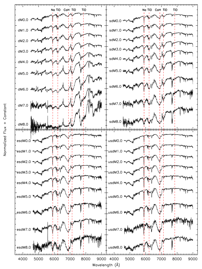
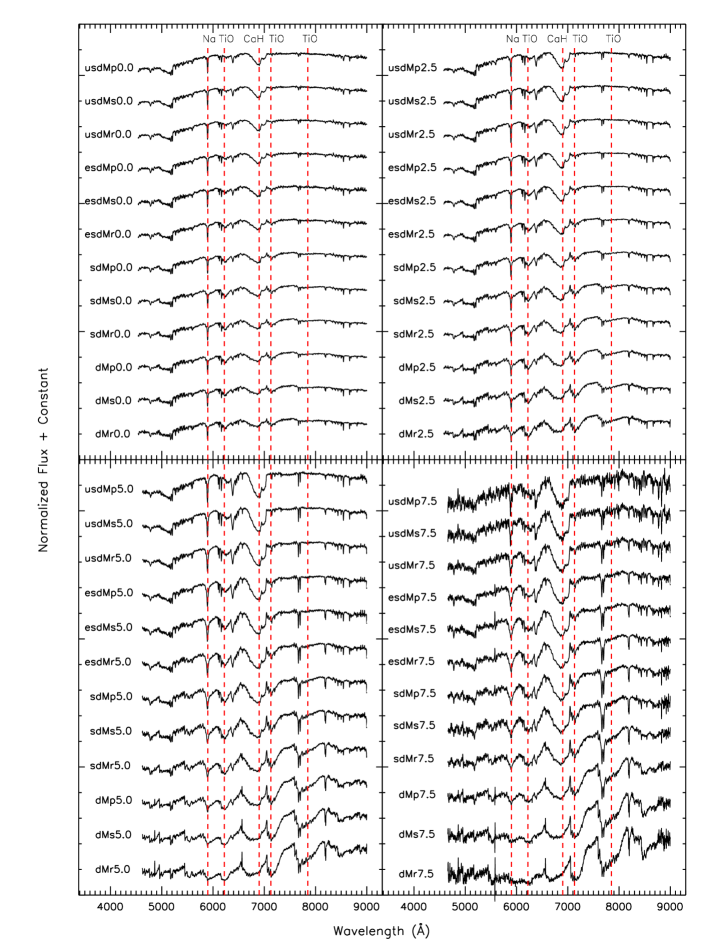
A subset of the final templates is presented in Figures  1 and  2. The resulting templates span the spectral subtypes K7.0-M8.5, and cover every half-subtype in those ranges. These initial templates are arranged in a two-dimensional grid, with one axis measuring the general strength of the molecular bands and the other axis measuring the ratio of the TiO and CaH band strengths. The first axis (spectral subtype) is presumed to be mainly correlated with a star’s effective temperature. The second axis, on the other hand, is presumed to be mainly correlated with a star’s metallicity, although this need not be strictly the case; for instance, the ratio of TiO to CaH can also be a function of surface gravity. In any case, we will assume that our classification system essentially represents a ”temperature-metallicity” grid. With over 18 elements of resolution in ”temperature”, and 4 elements of resolution in ”metallicity”. (We note that the term ”metallicity” is only used here to suggest that the variations in TiO to CaH band strength ratios are most likely due to variations in a star’s chemical composition. It is clear that these specific ratios may not be strictly correlated with the abundance of iron, so our use of the word ”metallicity” here is not meant to suggest that values of [Fe/H] can be inferred from those grids.) The limited resolution along the ”metallicity” axis is due in part to the difficulty in measuring accurate metallicity values in individual stars using the TiO5 and CaH2+CaH3 spectral indices alone, combined with the limited signal-to-noise ratio in the individual stars. Our co-added templates however provide significantly higher signal-to-noise, which make it possible to define a finer ”metallicity” scale.

To increase the number of metallicity grid points from 4 to 12, we used the following procedure. For any one of the four original metallicity classes (i.e., dM), each can be expanded to three subclasses: a relatively more metal-rich subclass (i.e., dMr), a standard subclass (i.e. dMs), and a relatively more metal-poor subclass (i.e., dMp). Assuming that the metallicity grid is a linear system (see more details in Mann et al., 2012), the extra synthetic templates can be created by extrapolating between two neighboring classes. For example, we can synthesize dMp templates by considering them to be one third of the way from the dM standard class to the sdM standard class:

$$[dMp]=\frac{[sdMs]-[dMs]}{3}+[dMs]=\frac{2}{3}[dMs]+\frac{1}{3}[sdMs]$$ (1)

where dMs and sdMs are the original template spectra of the dwarfs and subdwarfs. We can thus interpolate between dMs and sdMs to create dMp and sdMr subclass templates, between sdMs and esdMs to create sdMp and esdMr subclass templates, and between esdMs and usdMs to create esdMp and usdMr subclass templates. To create the dMr and usdMp templates, we can extrapolate them from the original templates assuming a linear progression at the edges. To make the dMr template, we can assume that the dMs template is between dMp and dMr, which means $dMs=([dMp]+[dMr])/2$, and using the Eq. 1, the dMr template can be derived:

$$[dMr]=2[dMs]-[dMp]=\frac{4}{3}[dMs]-\frac{1}{3}[sdMs]$$ (2)

And the usdMp subclass template can be similarly synthesized by the same extrapolation from the other edge.

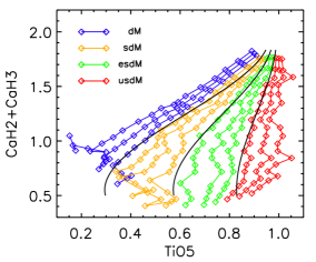
To verify the validity of our synthetic method, the distribution of TiO5 and CaH2+CaH3 spectral indices from all the synthetic templates is shown in Figure 3. Four different colors represent the four original metallicity classes, which are dwarfs (blue), subdwarfs (yellow), extreme subdwarfs (green), and ultra-subdwarfs (red), from left to right on the plot, respectively. For each metallicity class color, the middle line is the spectral index distribution of the corresponding original template sequence, while the leftmost line corresponds to the relatively more ”metal-rich” subclass sequence (r), and the rightmost line corresponds to the relatively more ”metal-pool” subclass sequence (p). The three black lines are the boundaries proposed by Lépine et al. (2013) to separate the four original metallicity classes. This shows that our synthetic templates not only define a finer ”metallicity” grid but also still follow the original classification criteria within each metallicity subclass. However, for later subtypes (dM7.0-dM8.5, sdM7.0-sdM8.5), the relative rarity of SDSS spectra having appropriate ”temperature” and ”metallicity” values results in the templates being dominated by the spectra of just a few stars, which can skew the mean ”metallicity” and ”temperature” of the subsample, due to fluctuations from small number statistics. On the other hand, the low S/N ratio of late-type template spectra also leads to larger errors in the measurement of spectral indices and limits their value as a subtype/metallicity test (Figure 3). Therefore, metallicity class estimates at the latest subtypes based on these templates should be used with caution.

We emphasize here again that we use the terms ”temperature” and ”metallicity” in our classification system as an educated suggestion for what we believe underlies the two dimensional classification grid. These are not meant to suggest that each grid point represents a unique combination of the physical parameters Teff and [Fe/H]. What this means is that this proposed classification system should be used for classification purposes, and not as a means to determine physical parameters for a star. The determination of physical parameters from this classification would first require a validation and calibration of the grid. This is in fact an ongoing area of research in the field of cool stars which has seen some progress in recent year, see e.g.,Rojas-Ayala et al. (2012); Mann et al. (2013, 2014); Newton et al. (2015). It should be understood in the following section that the term ”temperature” is used in the sense of ”spectral subtype”, the first axis in our classification grid, and that the term ”metallicity” is used to described the second axis in our classification system, which really describes molecular band ratios.

Figure 3.— Distribution of the TiO5 and CaH2+CaH3 spectral indices in the classification templates. The four colors represent the four original metallicity classes: dwarfs (blue), subdwarfs (yellow), extreme subdwarfs (green), and ultrasubdwarfs (red). Our templates further subdivide each metallicity class into three subclasses: relatively more metal-rich subclass(Mr), standard subclass(Ms), and relatively more metal-poor subclass(Mp), from left to right on the plot, respectively. Indices for the three subclasses are shown. Segments connect the index values of templates from the different spectral subtypes within each of the metallicity subclasses. The boundaries of the four metallicity subclasses, as proposed by Lépine et al. (2013) are shown as black lines. Although our templates were originally assembled by the Lépine, Rich, & Shara (2007) calibration, which makes a small offset between a few early-type synthetic templates and the boundary lines, the differences were not significant. Overall, our synthetic templates define a finer metallicity grid, while still following the original subclass separation.

Figure 4.— Distribution of estimated mean S/N ratio in the LAMOST spectra for 2,612 M dwarfs/subdwarfs. The sub-panel display the mean S/N distribution in the range $0<$S/N$<10$.

Figure 5.— Quality of the fit for a representative high S/N spectrum in the LAMOST commissioning data, identified to be an M3.5 dwarf by our template-fitting method. Top panel: the full spectrum, which is a composite of the LAMOST blue channel and red channel spectra. Bottom panels: the smoothed LAMOST spectrum (black) overlaid on classification templates selected to demonstrate the quality of the fit (red). Bottom left: Three adjacent templates of the same subtype but different metallicity subclasses. The middle one is the best fitting template; the one above is the relatively more metal-poor template, and the one below is the relatively more metal-rich template, as labeled. The difference between top/bottom templates and the LAMOST spectrum is clear in the 6000Å–6200Å, 6900Å–7100Å(CaH and TiO band) and 7400Å–7600Å(VO band) ranges. Bottom right: Three adjacent templates of the same metallicity subclass but different spectral subtypes. The middle one is the best fitting template, while those above/below represent templates of higher/lower temperatures in the sequence. The most significant difference is in the 6000Å– 6200Årange.

Figure 6.— Quality of the fit for a representative LAMOST spectrum of intermediate S/N. The star happens to be classified as sdMr2.5 by our pipeline. Panels are the same as in Figure 5, except that additional templates extending $\pm$1 metallicity subclasses and $\pm$1.0 spectral subtypes from the best fit are also shown for comparison.

Figure 7.— Quality of the fit for a typical LAMOST spectrum of low S/N. The star happens to be classified as an extreme subdwarf (esdMp0.0) by our pipeline. Because of the serious skylines contamination and the weakness of the molecular bands, it is hard for our template-fit method to classified the spectrum with the same accuracy as the higher S/N spectra shown in Figure 5 and Figure 6. In any case, close examination of neighboring templates (above and below the best fit template shown in the middle) reveals difference that are significant enough near the 7,000Åregion to be confident of a classification accuracy to within $\pm$1.0 spectral subtypes and within $\pm$2 metallicity subclasses.

Figure 8.— Distribution of the spectral index measuring the bandhead of the TiO band redward of 7040Å(TiO5) and the sum of the indices measuring the strength of the CaH bandhead blueward of 7040Å(CaH2+CaH3). Different symbols are used for stars classified in the LAMOST classification pipeline as dwarfs (dM), subdwarfs (sdM), extreme subdwarfs (esdM), and late-K dwarfs. As expected, many of the subdwarfs and extreme subdwarfs fall to the right of the dM dwarfs sequence, due to the TiO/CaH band ratio being metallicity dependent. Some stars classified as M subdwarfs have indices more consistent with dM dwarfs; those stars tend to have lower S/N and could be misclassified, or suffer significant measurement errors on the spectral indices. The three solid black lines delimitate the loci of the four metallicity classes (dM, sdM, esdM, usdM, left to right) originally proposed by Lépine et al. (2013). Two outliers, classified as dM dwarfs but falling outside the normal distribution of dM stars in this diagram (open blue triangle and diamond symbols), are investigated in Figure 9.

Figure 9.— Spectra of the two outlier stars marked in Figure 8. $Top$: spectrum of the outlier identified as an open triangle symbol. The weaker molecular bands of CaH, consistent with the location in the TiO/CaH diagram of Figure 8, indicate that it is most probably an M giant instead of an M dwarf. $Bottom$: spectrum of the outlier represented by an open diamond symbol. Because of the low S/N ratio, the skylines occurring in the CaH molecular bands result in significant errors in the spectral index measurements. The template-fit classification appears to be quite good however.

Figure 10.— Spectral index distribution of dM dwarfs for the three different metallicity subclasses defined in this paper. The different loci of the dMp, dMs, and dMr subclasses clearly show that the metallicity subclasses defined in our spectral fitting method also consistently separate out the stars in the spectral index grid, according the expected trends for metallicity variations.

Figure 11.— Distribution of the flux correction factor $fc$, which measure whether the spectral energy distribution of a LAMOST M dwarf looks redder ($fc<1$) or bluer ($fc>1$) than the adopted SDSS-based classification templates. The distribution suggests that the flux calibration is generally good for most of the LAMOST commissioning spectra, albeit redder than expected on average. To investigate the possibility of interstellar reddening, we divide the stars in two groups based on their spectroscopic distance. The closer stars tend to have relatively fewer outliers but still look marginally redder than expected, on average, which points to differences in the LAMOST and SDSS flux calibrations.

Figure 12.— Distribution of 2MASS J-H and H-K_s colors for the stars identified as late-K and M dwarfs/subdwarfs in the LAMOST commissioning data. $Left$: the 1,080 nearest stars ($d<300pc$); their relative concentration is consistent with unreddened main sequence stars as shows in the infrared color-color diagram of Lépine, & Shara (2005). This suggest that there is no significant interstellar reddening or red giants contamination. $Right$: the 1,497 more distant stars ($d>300pc$). The larger scatter is in part due to stars have fainter magnitudes, and thus larger uncertainty in their infrared colors. The distribution, however, also shows redder colors on average. This systematic offset suggests that some stars may suffer some form of interstellar reddening, which would be consistent with the larger distance range.

Figure 13.— Distribution of absolute magnitudes in J band for nearby M stars with both spectral subtypes and parallax distances. A random values of $\pm$ 0.1 subtype was added, to spread out the data for more clarity. Stars from different metallicity classes (dM, sdM, esdM, usdM) are shown in different panels. The black lines show the adopted relationships for each metallicity subclass.

Figure 14.— Distribution of spectroscopic distances for stars in three spectral subtype ranges (K7-M0, M1-M2, and M3-M5). The early-type dwarfs are dominated in our catalog and are sampled over a larger spectroscopic distances than other late-type dwarfs. This bias is entirely due to magnitude selection effects, which are expected because the early-type M dwarfs are intrinsically brighter than the late-type M dwarfs.

Figure 15.— Distribution of transverse velocities as a function of the spectroscopic distance. Mean velocities are calculated for stars in three distance bins (0-400 pc, 400-800 pc, 800-1200 pc); the red dots and error bars represent the median transverse velocity and the corresponding standard deviation for each bin. The mean transverse is largely consistent with the local kinematics of disk stars. However, it shows a weak growing trend with spectroscopic distance, which can be simply explained by the uncertainty in the spectroscopic distance estimates.

Distribution of UVW components of motion for our spectroscopically classified M dwarfs in LAMOST, based on spectroscopic distances and proper motion measurements using the method described in §5.5. Each M dwarf contributes only two velocity components, which means it is only shown in one of the panels. The (V,W) projection shows the expected asymmetric drift of local disk stars.

3.2. Method for template fitting

We perform our spectral classification by calculating the chi-square value between any one LAMOST spectrum and each of the template spectra. The spectra are first reduced using the LAMOST 2D pipeline (Luo et al. 2004), which includes bias subtraction, flatfield correction, skyline subtraction, wavelength calibration, and flux calibration (Zhao et al. 2012). For best results, we have determined that the spectral fitting should avoid the overlap region between the blue-channel and red-channel spectra, which is between 5700Åand 5900Å(Wu et al. 2011), because of noise and flux calibration issues. The spectral fit should also avoid the wavelength range between 8000Å – 9000Åwhere serious skyline contamination occurs. The spectral wavelength range used for the classification fit is thus limited to 6000Å–8000Å. Bad pixels, flagged by the LAMOST reduction pipeline, are also excluded from the fit. The chi-square for the $j$th template spectrum is defined as:

$$\chi_{j}^{2}=\sum_{i=1}^{N}\left(\frac{L_{i}-T_{ij}}{\sigma_{i}}\right)^{2}$$ (3)

where $L_{i}$ is the LAMOST spectral flux for each of the i=1,N pixels, $T_{ij}$ is the flux of the $j$th template spectrum for every corresponding pixel $i$, and $\sigma_{i}$ is the error for the LAMOST spectral flux at each pixel $i$. N is equal to 1250 because there are 1250 pixels between 6000Åand 8000Å.

In order to correct for radial velocity shifts, and reduce the possible effects of faulty wavelength calibration (See §2 above), we have to makesure that the stars are classified in their local rest frame as much as possible. We therefore shift each LAMOST spectrum towards the blue or red by an integer number of pixels, and recalculate the chi-square value against each template spectrum. For each LAMOST spectrum, we allow for a possible maximum shift of $\pm$8 pixels, which corresponds to maximal radial velocity shifts of approximately $\pm$550 km/s. The factor combination of pixel shifting and $j$th template spectrum which gives the minimum chi-square value is selected as the best fit.

Stars are rejected when their best fit is a match to a non-M dwarf template. For each of the 12 metallicity subclasses, there are two earlier template spectra (called non-M dwarf templates) corresponding to K5.0 and K5.5 dwarf/subdwarf subtypes; these templates have extremely weak molecular features of titanium oxide (TiO), vanadium oxide (VO) and calcium hydride (CaH). For stellar types earlier than K7.0, these molecular bands are indeed so weak as to be generally undiscernible, except in spectra with very high S/N, and the spectra essentially all look relatively flat in the 6000Å– 8000Årange (Reid, Hawley, & Gizis 1995). As a result, any star with a subtype earlier than K7 (including all F and G stars) will have its best match with any one of the K5.0 or K5.5 templates. Any star with a best match to those templates is therefore identified as a non-M dwarf, and rejected.

Since the quantum efficiency for CCDs in LAMOST is increasing over the wavelength range from 6000Åto 8000Å, the measurement errors for each pixel have a systematically decreasing trend over this wavelength range. So when we use the LAMOST spectrum’s chi-square fit to the template, the red part close to 8000Åhas more weight than the blue part closer to 6000Å. On the other hand, most of the prominent molecular absorption features are in this bluer part. This means that some non-M dwarf stars which happen to have similar spectra on the red side around 8000Åmight be classified as M dwarfs, even if there is no good fit on the blue side. This is more common for low S/N spectra, because their blue edge is dominated by the instrumental noise, and their red edge is as featureless as most of the templates, and thus they appear more similar to the early-M dwarf templates than to the late-K ones.

To solve this problem, we use an additional criterion to identify and reject non-M dwarfs with noisy spectra that might otherwise be classified as M dwarfs from the chi-square fit. In addition to the chi-square value, we also calculate the integrated square of the difference between the LAMOST spectrum and the best classification template. If the integrated square difference is greater than 130 pixel units, then the star is considered a non-conclusive classification and is excluded from the final M dwarf list. Specifically, this means that we allow for a maximum difference between a LAMOST spectrum and a classification template of 10% for each pixel on average; for the normalized spectra, the corresponding difference is 0.1 units. Because there are about 1250 pixels used in the fit, the threshold value in the fitting area is about 130 pixel units. Our experience shows that this procedure eliminates the vast majority of noisy, but clearly non-M dwarf stars that may otherwise be identified as M dwarfs from the chi-square fit.

3.3. Additional Spectrophotometric Correction

We find that to obtain the best results with our template fit methods, both the LAMOST spectra and the classification templates also need to be flux-normalized before the fit, i.e. the spectra and templates need to be rectified with respect to a pseudo-continuum level. This ensures that the classification is primarily based on the absolute and relative strength of the molecular bands, and not on the slope of the spectral energy distribution, which can be affected by many factors such as errors in instrumental flux calibration, aperture losses combined with atmospheric differential refraction, or interstellar reddening.

Considering that the molecular bands completely dominate the spectral energy distribution within the fitting area, it is hard to objectively define a continuum for rectification. We therefore use a more simple flux recalibration that plays a similar role and performs a first order correction of the slope.

For each spectrum, we divide the spectral fitting range in two parts, and calculate the integrated flux within each of these two regions. Then the straight line $y=ax+b$ that fits the two median flux points is used to calibrate the flux and the slope of this spectrum. The parameters $a$ and $b$ are given by: $a=(F_{\rm r}-F_{\rm b})/(\lambda_{\rm r}-\lambda_{\rm b})$, $b=F_{\rm b}-a\lambda_{\rm b}$, where $F_{\rm r}$ is the median flux of the red section (7000Å-8000Å), $F_{\rm b}$ is the median flux of the blue section (6000Å-7000Å), and $\lambda_{\rm r}$, $\lambda_{\rm b}$ are the median wavelengths within each of the two regions. The same flux recalibration is performed on all the classification templates, and the chi-square best fit is performed for the normalized spectrum as it is fit on the normalized templates.

To evaluate the magnitude of this flux correction, we first define $R$ as the ratio of the spectral fluxes, $R=F_{\rm r}/F_{\rm b}$, where $F_{\rm r}$, $F_{\rm b}$ are the median fluxes which have been defined before. We then introduce $fc$ as the ratio of the red/blue flux ratio R for the original LAMOST spectrum (i.e. before flux correction) and the red/blue flux ratio R for the classification template which provides the best fit to the data (with the fit performed after flux recalibration). This factor of the flux correction $fc$ is thus defined as:

$$fc=\frac{R_{\rm LAMOST}}{R_{\rm SDSS}}$$ (4)

where $R_{\rm LAMOST}$ is the spectral flux ratio of the LAMOST spectrum and $R_{\rm SDSS}$ is the flux ratio of the classification template. Using this flux correction factor, we can verify whether the LAMOST flux calibration and SDSS flux calibration are similar ($fc=1$), indicating that the LAMOST spectrum has the same measured spectral energy distribution as an SDSS spectrum of the same spectral subtype. A value different from $fc=1$ would indicate that star has a spectral energy distribution that is different than that of a classification standard star of the same spectral type. The value of $fc$ can thus be used, e.g., to diagnose reddening in a star, which would produce a value of $fc<1$.

Again, the final template fit is performed after these additional flux corrections. Stars which are found to match one of the templates are then automatically assigned a metallicity class (dMr, dMs, dMp, sdMr, sdMs, sdMp, esdMr, esdMs, esdMp, usdMr, usdMs, usdMp) and spectral subtype (0.0 to 8.5) from the class and subtype of the template which provided the best fit. We also include stars classified with subtypes K7.0 and K7.5, and of all metallicity subclasses.

4. Application and Verification of the Classification Method

4.1. Search results

We performed spectral classification of all the spectra collected during the LAMOST commissioning phase, using our template-fit method. Of the 83,500 spectra which were passed through the M dwarf classification pipeline, 2,612 were positively identified as M dwarfs/subdwarfs by our classification code, 74,573 spectra (89.3%) were excluded as non-M dwarfs by the template fitting method, and 6,315 spectra (7.6%) were rejected as too noisy for classification, based on our integrated square-difference criterion.

Superficial examination of the spectra from the 2,612 M dwarf candidates shows that all of them display TiO and CaH bands, which confirms that they are all consistent with M dwarf/subdwarf stars. Examination of some of the 80,888 rejected spectra, on the other hand, reveals a variety of other sources, some looking like stars of earlier spectral types such as AFGK stars and white dwarfs, others showing only sky lines, or spectra that are too noisy to be identified. In any case, none of the rejected spectra are found to show clear evidence of TiO or CaH molecular bands, and are thus not M stars.

4.2. Sample spectra

To verify the quality of the template fits and how effectively M dwarfs/subdwarfs are classified with our pipeline, we performed close visual inspection of a number of spectra covering a broad range of spectral subtypes (as determined from our fit) and with a range of integrated square differences to the classification template.

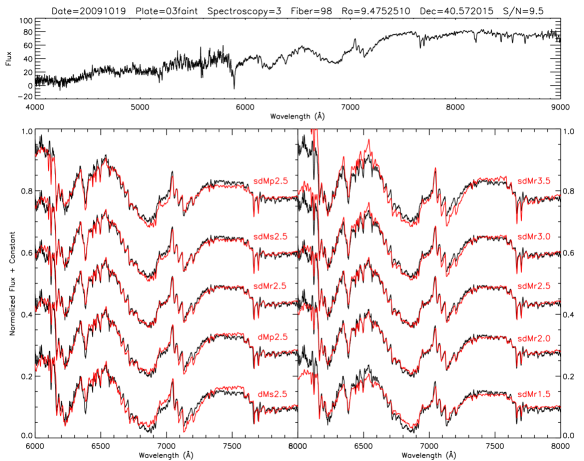
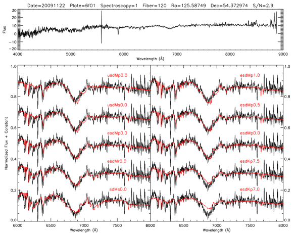
Since the classification accuracy is mainly influenced by the S/N ratio for each spectrum, the S/N distribution for 2,612 M dwarfs/subdwarfs is shown in Figure 4. Based on this histogram, we can divide the M dwarfs/subdwarfs classified in our pipeline into three subsets: the high S/N spectra ($S/N>15$), the intermediate S/N spectra ($5<S/N<15$), and the low S/N spectra ($S/N<5$). To illustrate the fit quality of different S/N subsets, we plot three example spectra and their fitting templates in Figures 5, 6, and 7.

Figure 5 displays the LAMOST high S/N spectrum of a star classified as dM3.5 by our pipeline (black line). The spectrum is compared to the best-fitting template (red line). The best-fitting template (dM3.5) shows a near-perfect fit to the LAMOST spectrum, and in particular is an excellent match to the main molecular absorption bands (TiO, CaH) between 6000Åand 8000Å. To evaluate the quality of the fit, we also compare this LAMOST spectrum with the four adjacent templates in the spectral subtype / metallicity class grid, which are overlaid on the LAMOST spectrum. There are subtle but clear differences between each of these adjacent templates and the LAMOST spectrum, which demonstrate that the class/subtype dM3.5 provides the best possible classification for the star. This suggest that for high-quality data, our classification method is indeed accurate at least to the nearest half-subtype, and to the nearest metallicity subclass.

Figure 6 shows the case of a LAMOST spectrum of intermediate S/N, which happens to be identified as an M subdwarf, with a sdMr2.5 classification. Although the differences between early-type dwarfs in the temperature-metallicity grid are not as clear as for the dMs3.5 star in Figure 5, there are still notable differences which indicate that the fit is not as good for the adjacent templates. With the differences between the LAMOST spectrum and the templates increasing significantly for templates beyond those displayed in Figure 6, we remain confident that the classification also has an accuracy of at least +/-0.5 subtypes, and is accurate to within the nearest metallicity subclass.

Figure 7 shows the low S/N spectrum of a LAMOST star, identified as an extreme subdwarf with a classification esdMp0.0 according to our code. The weakness of the molecular bands and the lower S/N makes it harder for the star to be accurately classified, and there is more uncertainty in the assigned spectral type and metallicity class. In any case, there are significant differences between the star and templates that are two steps away from the assigned subtype/subclass. From this we are confident that the classification is still accurate to within +/- 1.0 subtypes, and to within $\pm$2 metallicity subclasses.

Our pipeline has classified 2,612 M dwarfs/subdwarfs in total. The accuracy for low S/N spectra classification are no better than $\pm$1.0 subtype or $\pm$2 metallicity subclasses as defined in this paper, however these low S/N spectra (S/N ¡5) are a minority and only represent 25.8% of the catalog (675 stars). The remaining 1,937 stars have spectra with sufficient S/N ratio (¿5) to be accurately classified to within $\pm$0.5 subtype or $\pm$1 metallicity subclass.

4.3. Measurement of spectral indices

As an additional verification of our classification method, we have calculated sets of spectral indices commonly used for M dwarf/subdwarf classification. The TiO5, CaH2, and CaH3 spectral indices, as defined in Reid, Hawley, & Gizis (1995), were calculated for all the LAMOST stars identified as M dwarfs/subwarfs by our classification pipeline.

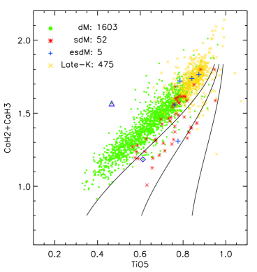
The distribution of TiO5 against CaH2+CaH3 was originally used to formally separate metal-poor M subdwarfs from metal-rich M dwarfs (Gizis, 1997; Lépine, Rich, & Shara, 2003, 2007). We plot this distribution for all the LAMOST M dwarfs/subdwarfs in Figure 8, using different symbols/colors for stars of different metallicity classes. We note that the distribution is in good agreement with Figure 3 of Lépine, Rich, & Shara (2007), and confirms that most of the LAMOST stars are relatively metal-rich M dwarfs and late-K dwarfs. The LAMOST stars classified as subdwarfs generally have higher TiO5 index value for a given range of CaH2+CaH3 values, also in general agreement with the spectral index classification system.

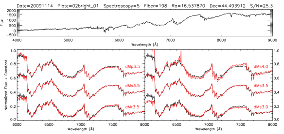
However, there are several outliers, e.g., stars classified as dM by our pipeline but with a [TiO,CaH2+CaH3] index more consistent with an sdM subtype. We carefully examine two of these to understand the discrepancy. The two stars represent two different kinds of offset along the dM sequence. The top panel of Figure 9 displays the spectrum of the star identified as an open triangle symbol in Figure 8. The difference in the molecular absorption bands between the star and any of the dM templates suggests that it is probably an M giant instead of M dwarf; the weaker molecular bands of CaH are consistent with the M giant spectra analyzed by Mann et al. (2012). In this particular example, it is our classification pipeline that is in error, and the TiO/CaH spectral index ratio more correctly identifies the star as M giant. It is hard for our automated classification pipeline to exclude these M giant stars with the template-fit method, because the dwarf templates always provide the best fit to the spectra and the molecular bands are similar. Our best option would be to use M giant templates in addition to the M dwarfs/subdwarfs. Future efforts will be devoted to adding M giant templates to the pipeline.

The second outlier, represented by a diamond symbol in Figure 8, is plotted in the bottom panels of Figure 9. Here the source of the offset is found to be due to instrumental factors. The low S/N ratio and intense skyline contamination in this spectrum cause a large error in the measurement of the spectral indices. In this case, it is the spectral index measurements that are in error, and our template fit method provides a more reliable estimate of the subtype and metallicity class.

More generally, we find that the spectral-fit method provides a better estimate of the spectral subtype because it uses a much broader wavelength range, whereas the TiO5, CaH2, and CaH3 spectral indices are narrowly defined, and thus much more sensitive to instrumental noise or spectral reduction artefacts. We find that large scatter of the sdM stars in Figure 8 is thus largely due to errors in the measurement the spectral indices from low S/N spectra, not in errors in our spectral classification pipeline. We conclude suggests that our classification pipeline is more reliable for measuring the spectral type and the metallicity than if we were using the spectral indices alone.

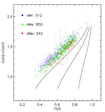
To verify the consistency of our newly introduced metallicity subclasses (r,s,p), we plot the spectral index distribution of dM dwarfs for the three different subclasses in Figure 10. The slightly different locations (layering) of the dMp, dMs, and dMr stars suggest that the metallicity subclasses defined in our spectral fitting method also consistently separate out the stars in the spectral index grid following the expected trends for metallicity variations, with the more metal-rich stars (dMr) having lower TiO5 values for a given CaH2+CaH3, and the more metal-poor stars (dMp) having higher TiO5 values.

Table 3 The absolute magnitude ($M_{J}$) for spectral subtypes (SpTy)

	d…	sd…	esd…	usd…
…K7.0	5.600	6.050	7.400	8.550
…K7.5	5.800	6.425	7.600	8.675
…M0.0	6.000	6.800	7.800	8.800
…M0.5	6.200	7.175	8.000	8.925
…M1.0	6.400	7.550	8.200	9.050
…M1.5	6.600	7.925	8.400	9.175
…M2.0	6.800	8.300	8.600	9.300
…M2.5	7.000	8.675	8.800	9.425
…M3.0	7.450	9.050	9.000	9.550
…M3.5	7.900	9.425	9.200	9.675
…M4.0	8.350	9.800	9.400	9.800
…M4.5	8.800	9.950	9.600	9.925
…M5.0	9.250	10.100	9.800	10.050
…M5.5	9.700	10.250	10.000	10.175
…M6.0	10.150	10.400	10.200	10.300
…M6.5	10.325	10.550	10.400	10.425
…M7.0	10.500	10.700	10.600	10.550
…M7.5	10.675	10.850	10.800	10.675
…M8.0	10.850	11.000	11.000	10.800
…M8.5	11.025	11.150	11.200	10.925
…M9.0	11.200	11.300	11.400	11.050
…M9.5	11.375	11.450	11.600	11.175

4.4. Flux correction

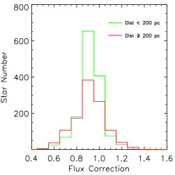
As we defined in Section 3.3, the flux correction, $fc$, is mostly useful to verify the quality of the LAMOST flux calibration. Figure 11 shows the distribution of $fc$ values for all 2,612 stars classified as M dwarfs/subdwarfs. The distribution suggests that the flux calibration is in general agreement with the SDSS calibration for most of the LAMOST commissioning spectra. However, we find a median value of $fc<1$, which suggests that the LAMOST spectra have systematically redder spectral slopes than the SDSS spectra for stars of the same spectral subtypes. We suspect this is due to minor flux calibration differences between the LAMOST and SDSS data reduction pipeline. The tails in the distribution, on the other hand, are mainly due to LAMOST spectra with instrumental issues or data reduction/calibration shortcomings. The left wing (low $fc$ values) comprises stars in which there is an over-subtraction of the sky lines, which makes the stars appear systematically redder. The right wing of the distribution (high $fc$ values) comprises spectra which suffer from a known issue with the blue channel calibration, making the stars appear bluer.

Interstellar reddening might also be affecting the distribution to some extent, although the effect should be small given that most of these M dwarfs are relatively nearby. To examine this possibility, we separately plot in Figure 11 the distribution of $fc$ values for the relatively nearby (d$<$200pc) and the more distant (d$>$200pc) M dwarfs in our list (see below). We find no significant offset between the two distribution, which suggests that interstellar reddening is negligible within our larger catalog, and that most of the $fc$ values correct for instrumental errors in the spectrophotometry.

4.5. Infrared color distribution

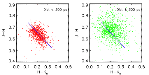
One potentially serious source of contamination in any red dwarf survey are background red giant stars, which also display molecular bands of TiO, CaH, and VO, similar to the M dwarfs. To identify possible red giants in our sample, we examined the 2MASS J-H and H-K_s colors, of all the stars identified as M dwarfs/subdwarfs by our pipeline. M giants occupy a distinct locus in the (J-H, H-K_s) diagram (Bessell & Brett, 1988; Lépine, & Shara, 2005); this is due to the development of water bands in M dwarfs which depresses the flux in the H and K_s bands and make the dwarfs appear bluer. In particular, M dwarfs always show $J-H<0.7$, while giants usually have much redder $J-H$ colors.

The (J-H, H-K_s) distribution of the stars identified as M dwarfs/subdwarfs by the LAMOST pipeline is plotted in Figure 12. Stars are plotted in two separate subsets based on their spectroscopic distance (see §5 below). The nearest stars ($d<200pc$) occupy a relatively concentrated area which is remarkably similar to the unreddened nearby M dwarfs locus in the (J-H, H-K_s) diagram by Lépine, & Shara (2005). The agreement suggest that there is probably no significant interstellar reddening, no significant contamination from red giant stars. The distribution of the more distant stars ($d>200pc$), on the other hand, in the (J-H, H-K_s) diagram shows significantly more scatter, and also displays a systematic average shift to redder infrared magnitudes, with many stars having colors $J-H>0.7$. While this could be indicating the presence of some red giant contaminants, this possibility is not supported by the distribution of spectral indices. After careful examination of all the LAMOST spectra for stars with $J-H>0.7$, we conclude that the vast majority of the stars are indeed M dwarfs and not M giants, with the notable exception of the star shown in Figure 9 and discussed above.

Instead, we suggest that the systematically redder colors may indicate true interstellar reddening at least in some stars. This is supported by the fact that the offset affects mostly the more distant stars in our list. This reddening would have been corrected in our flux renormalization procedure, and go unnoticed. In addition, the increased scatter may be explained by the fainter infrared magnitudes of the more distant M dwarfs. Overall, this indicates that giant star contamination is not a significant problem in our M dwarfs/subdwarfs catalog.

5. Distance and Kinematics analysis

5.1. Spectroscopic distances

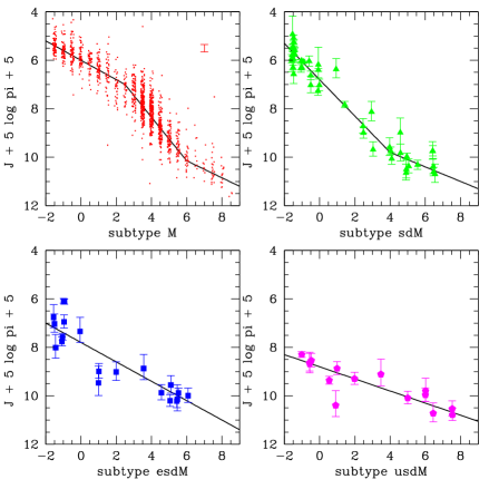
Spectroscopic distances for the stars were estimated based on the absolute infrared magnitude (MJ) to the spectral subtype (SpTy) relationships. These relationships were re-calibrated using a revised census of nearby M dwarfs with both spectral types and parallax distances, which we assembled. We first identified M dwarf and M subdwarf stars with parallax measurements documented in Monet et al. (1992); Harrington et al. (1993); van Altena et al. (1995); Henry et al. (2006); van Leeuwen (2007); Gatewood & Coban (2009); Lépine et al. (2009); Smart et al. (2010); Khrutskaya et al. (2010); Riedel et al. (2011); Jao et al. (2011); Dittmann et al. (2014), with a smaller number of additional stars from Lépine et al.(2015, in preparation). Within this sample, we identified 1459 stars with known spectral subtypes as determined in Reid, Hawley, & Gizis (1995); Lépine, Rich, & Shara (2003, 2007); West et al. (2011); Lépine et al. (2013); with again some additional subtypes determinations from Lépine et al.(2015, in preparation). The final calibration sample includes 1374 dM, 47 sdM, 21 esdM, and 17 usdM. The distribution of absolute J magnitudes as a function of the spectral subtype is shown in Figure 13, with one panel for each of the metallicity classes. For every star, random values of $\pm$ 0.1 subtype was added, to spread out the data for more clarity.

The absolute magnitude to spectral subtype relationship for esdM and usdM stars was determined with a simple fit of a linear function. For sdM stars, we found a simple linear fit to be unsatisfactory due to an apparent inflection point at later subtypes, and instead determined a calibration using two linear segments. For M dwarfs, even the two-segment fit proved unsatisfactory, and a three segment calibration was determined instead. Those relationships are plotted in Figure 13. The corresponding values for the absolute J magnitude as a function of subtype are listed in Table 3. We estimate that this calibration provides values of MJ with an uncertainty of about 0.7 magnitudes, yielding spectroscopic distances with an accuracy of about 40%.

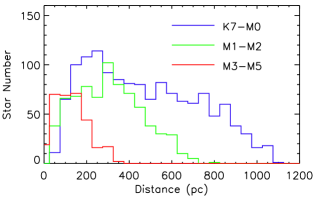
Figure 14 shows the distribution of spectroscopic distances for stars in various ranges of spectral subtypes. Early-type red dwarfs (K7-M2) are clearly detected over a much larger distance range than mid-type objects (M3-M5), which is as one should expect from the magnitude limit of the LAMOST survey. Only in the first distance bin ($d<100pc$) are mid-type M dwarfs significantly more numerous that early-type ones. This suggests that the vast majority of M dwarfs that will be observed and classified in the LAMOST survey will be early-type M dwarfs at least to within about 500pc of the Sun. For mid-type M dwarfs, the survey will only probe the volume within about 100pc of the Sun.

5.2. Proper motions

We obtained proper motions for most of the K/M dwarfs by searching the PPMXL catalog of Roëser et al. (2010) and the latest version of the SUPERBLINK proper motion catalog (Lépine, & Shara, 2005; Lépine & Gaidos, 2011). We used the positions of the stars in the LAMOST input catalog to search for the positions in PPMXL of the LAMOST K/M dwarfs identified in our pipeline, finding matches for 2,458 stars. Then we used the SUPERBLINK catalog to match the rest of the 154 stars, which provided proper motions for an additional 30 stars. Proper motions could not be assigned for the remaining 124 sources. The proper motion range for K/M dwarfs in our catalog is 1 mas yr^-1 $<\mu<$ 416 mas yr^-1, while the median value of the proper motion is 21 mas yr^-1.

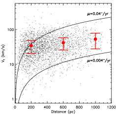
These proper motions can be used to validate our spectroscopic distances, to the extent that the calculated transverse motion should be consistent with the known, local kinematics of the Galactic disk. The distribution of transverse velocities is plotted in Figure 15 as a function of the spectroscopic distance. We find that most of the stars have transverse motions in the 10-100 km s^-1 range, which is indeed largely consistent with the local disk kinematics. The more distant stars (according to our spectroscopic distance measurements) are also found to have significantly smaller proper motions, which is also as expected. We also do not see any significant number of objects with unusually small transverse motions, which is what one would expect if background M giants were contaminating the sample, because misclassified giants would also have significantly underestimated spectroscopic distances.

We measure the mean value of the transverse motion for stars in three bins of spectroscopic distances ($d<400pc$, $400pc<d<800pc$, $800pc<d<1200pc$), along with the dispersion about the mean. These are plotted in Figure 15. All values are consistent with a mean velocity dispersion of $\sim 40$km s^-1, but there is a hint of a monotonic increase of the mean transverse velocity with distance. This can be explained by uncertainties in the spectroscopic distances: stars with underestimated distances will also have underestimated transverse motion, and stars with overestimated distances will also have overestimated transverse motions. Stars in the most distant bin have mean transverse motions about $40\%$ larger than the stars in the central bin (55 km s^-1 compared with 40 km s^-1); this suggests that spectroscopic distances may be over- or under-estimated by about $\pm$40% as well. This caveat should be considered when conducting a kinematical analysis of the M dwarfs detected in LAMOST.

5.3. Distribution of space motions

We could not obtain radial velocities for the K/M dwarfs we identified due to unreliable wavelength calibration of the LAMOST commissioning spectra. With the improvement of instrument and calibration method in regular survey, the radial velocity estimates for K/M dwarfs are expected to be available for upcoming data releases.

While the unavailability of radial velocity measurements limits the amount of kinematical data, it is still possible to carry out basic kinematics analysis from spectroscopic distances and proper motions alone. This can be done using the statistical method described in Lépine et al. (2013), in which it is assumed that the radial velocity $R_{V}=0$ for all K/M dwarfs, but different subsets are extracted to study the velocity distribution in various projections of the local (U,V,W) velocity space. Here we assume U is the component on motion pointing in the direction of the Galactic center, V the component in the direction of Galactic rotation, and W in the direction of the north Galactic pole. The statistical method uses the fact that in some specific directions on the sky, it is possible to calculate 2 of the 3 components of motion using distances and proper motions alone. For example one can measure the components U and V from proper motions and distances if the stars are in close proximity to the north or south Galactic poles (because the radial velocity contributes almost exclusively to the component W). Likewise the components of U and W can be measured from distances and proper motions alone for stars located in close proximity to the Galactic center and anti-center, and the components of V and W can be measured from distances and proper motions alone for stars located in close proximity to the apex and antapex of the Galactic rotation ($l=90,b=0$; and $l=270,b=0$). The approximation however breaks down for stars that are far from any of those six points on the sky, but can be efficiently used in large surveys for specific subsets.

Here we adopt the following approach: for every star in the sample, we determine which of the six canonical points (as described above) is closest to the star in question, and calculate the two components of motion which can be approximated with distance and proper motion alone for stars close to that point on the sky. Effectively this means that a single pair of components of motion (either UV, UW, or VW) is calculated for each star, is every case assuming that the radial velocity is zero. Because the LAMOST commissioning data only covers fields of low galactic latitudes, this means that all stars get either estimates of (U,W) or of (V,W).

These distributions are shown in Figure 3.1. It is interesting that the (V,W) distribution clearly displays the expected local asymmetric drift, with most stars having $V<0$km s^-1. The (U,W) distribution, one the other hand, suggestively shows a non-isotropic structure which could possibly be the signature of local streams, although further analysis would be required, ideally with the inclusion of radial velocity measurements, to confirm whether this trend is real.

While this method does not provide complete (U,V,W) component for any one of the stars, we still have sufficient numbers of stars contributing information to each of the three velocity components. Simply, stars with blanked values in one component of motion are not used to calculate the statistical moments of that component. The mean velocity and standard deviation for the (U,V,W) components are therefore calculated to be:

$$<U>=-9.8\pm 1.4~{}{\rm kms^{-1}},\sigma_{U}=35.6\pm 6.1~{}{\rm kms^{-1}},$$

$$<V>=-22.8\pm 0.7~{}{\rm kms^{-1}},\sigma_{V}=30.6\pm 2.0~{}{\rm kms^{-1}},$$

$$<W>=-7.9\pm 0.5~{}{\rm kms^{-1}},\sigma_{W}=28.4\pm 3.3~{}{\rm kms^{-1}}.$$

Where the uncertainties are estimated by bootstrap method.

Comparing with other reported results, such as Hawley et al. (1996) for the PMSU survey, Fuchs et al. (2009) for the SDSS survey, and Lépine et al. (2013) for the SUPERBLINK survey, our (U,V,W) velocity components are general consistent with those values. The agreement further suggests that our spectroscopic distance estimates do not suffer from systematic error, and are reliable enough to conduct kinematic studies. This opens the prospect of using large numbers of spectroscopically confirmed M dwarfs from LAMOST to perform massive kinematics studies of the nearest 1kpc.

6. Description of the catalog

The complete catalog of 2,612 M dwarfs/subdwarfs is provided in Table 4. Columns 1 and 2 catalog list celestial coordinates at the 2000.0 epoch. Columns 3 to 6 list proper motions along the Right Ascension and Declination, in milliarcseconds per year, along with the measurement errors, when available. A flag indicating the source of the proper motion is included in column 7. Columns 8 to 13 tabulate the infrared J, H, K_s magnitudes of the counterparts in the 2MASS survey; 22 M dwarfs do not have 2MASS magnitude because they are too faint to be observed by 2MASS. Spectral subtypes which determined by our template-fitting classification code are tabulated in column 14. Based on the spectral subtypes, the estimated spectroscopic distances is listed in column 15.

7. Conclusions

We have successfully tested a template-fitting method to automatically identify and classify the late-type K and M dwarfs in spectra from the LAMOST survey. As an alternative to the classification software ’Hammer’, used to analyze Sloan Digital Sky Survey spectra, our procedure can perform more reliable spectral classification without the need for time-consuming, visual inspection. Instead of relying on the spectral indices measurement, we have assembled a set of classification templates by combining spectra of M dwarfs/subdwarfs in the Sloan Digital Sky Survey. The well-defined templates define a temperature and metallicity grid, which reliably classifies the LAMOST stars into subtypes (temperature) and metallicity subclasses by the template-fit method. The method relies on a spectrophotometric renormalization, which makes the fit less dependent of the observed spectral energy distribution of the star, and more dependent on the absolute and relative depths of the TiO, CaH, and other molecular bands.

To improve on the classification of M dwarfs/subdwarfs, we introduce subdivisions in the ”metallicity” class system, going from 4 main classes (dM, sdM, esdM, usdM) to 12 ”metallicity” subclasses, with the induction of three subdivisions for every metallicity class, labeled “r” for “richer”, “p” for “poorer”, and “s” for “standard”. These subdivisions are included are suffixes to the existing metallicity classes, thus providing a metallicity sequence which runs [dMr, dMs, dMp, sdMr, sdMs, sdMp, esdMr, esdMs, esdMp, usdMr, usdMs, usdMp], from the presumably most metal-rich to the more metal-poor star. The term ”metallicity” is used here in a suggestive manner, and should not be understood in the strict sense. The ”metallicity” axis in our classification system is mainly dependent on the TiO to CaH molecular band ratio, which is only assumed to be correlated with the star’s metallicity. Whether these ”metallicity classes” can be used to determine actual [Fe/H] values for each star would first require a proper calibration and validation of the classification grid, which is beyond the scope of this paper. In other words, the proposed classification system should be used simply for classification purposes at this time.

Using the LAMOST commissioning data acquired in 2009-2010, we identified 2,612 M dwarfs/subdwarfs by our classification pipeline, including 1,603 M dwarfs (dM), 52 metal-poor M subdwarfs (sdM), 5 very metal-poor extreme subdwarfs (esdM), and 1 probable ultra metal-pool subdwarf (usdM). Our quality controls and close examination of individual stars indicate that the typical accuracy for our template-fit method spectral classification to $\pm 0.5$ subtypes and to within 1 metallicity subclass (in the 12-subclass system). A complete list of the 2,612 M dwarfs/subdwarfs is provided in a table.

Contamination by background giant stars is shown to be negligible in this subset. The distribution of infrared colors and the relative strength of TiO and CaH molecular bands are inconsistent with significant red giant contamination, although one star is indeed identified (and flagged) as a probable giant.

To demonstrate proof-of-concept for using the LAMOST data for kinematics studies, we estimated the spectroscopic distances and heliocentric (U,V,W) velocity components to perform the kinematic analysis for all M dwarfs/subdwarfs we identified. A spectroscopic distance calibration is provided, which is based on collated parallax data for M dwarfs and M subdwarfs in the literature. Transverse motions are then calculated using proper motion data collected mainly from the PPMXL and SUPERBLINK proper motion catalogs.

This preliminary work therefore demonstrates that future LAMOST survey programs hold the potential to identify and classify very large numbers of M dwarfs in all parts of the sky, and the data collected will be of sufficient quality to obtain metallicity and kinematics information on local M dwarfs to a distance of at least 500 parsecs. The anticipated data hold the promise to considerably expand the statistics of the local M dwarf/subdwarf populations.

Table 4M dwarfs catalog,including astrometry,photometry, spectroscopic distances and estimated subtypes

RAJ2000	DEJ2000	pmRA	pmDE	e$\_$pmRA	e$\_$pmDE	fl	J	e$\_$J	H	e$\_$H	Ks	e$\_$Ks	subtype	Dist
deg	deg	mas/yr	mas/yr	mas/yr	mas/yr		mag	mag	mag	mag	mag	mag		parsec
18.561404	43.167682	7.4	-13.9	3.9	3.9	P	14.23	0.03	13.56	0.03	13.37	0.04	dKp7.5	485$\pm$145
17.613458	43.683223	-0.2	-7.9	4.0	4.0	P	15.67	0.07	15.00	0.08	14.67	0.09	dMs1.5	651$\pm$195
16.418509	43.924841	-3.6	-2.9	4.1	4.1	P	15.79	0.07	15.02	0.06	14.78	0.08	sdMs0.0	626$\pm$188
9.583018	40.944141	14.5	-16.0	3.8	3.8	P	12.16	0.02	11.47	0.03	11.30	0.02	sdMs0.0	117$\pm$ 35
16.169814	43.944604	-3.3	-14.4	5.7	5.7	P	15.96	0.09	15.41	0.09	15.21	0.11	dMs0.0	982$\pm$294
17.184962	43.590305	5.6	-10.8	4.0	4.0	P	15.43	0.05	14.76	0.05	14.50	0.06	dMr0.5	701$\pm$210
8.997519	41.646745	-45.5	-15.5	4.0	4.0	P	12.56	0.02	11.95	0.02	11.73	0.02	dMs1.5	155$\pm$ 46
11.176808	41.781084	-79.4	-16.2	4.0	4.0	P	12.22	0.02	11.66	0.02	11.44	0.03	sdMr1.0	85$\pm$ 25
11.422563	41.869348	-27.0	-23.2	4.0	4.0	P	12.98	0.02	12.36	0.02	12.19	0.02	esdKp7.0	130$\pm$ 39
123.894386	56.428029	1.5	8.8	4.0	4.0	P	12.78	0.02	12.08	0.02	11.97	0.02	dKs7.5	248$\pm$ 74
124.445228	56.492803	12.5	-98.0	4.0	4.0	P	11.88	0.02	11.28	0.02	11.13	0.02	dKr7.0	180$\pm$ 54
18.985212	44.650124	-24.4	-6.9	3.9	3.9	P	13.12	0.02	12.42	0.02	12.21	0.02	dMs0.5	242$\pm$ 72
17.300816	47.198761	-15.9	-6.3	4.0	4.0	P	14.41	0.04	13.76	0.04	13.64	0.04	dKr7.0	579$\pm$173
16.860019	47.571482	-12.8	-7.1	4.0	4.0	P	13.43	0.02	12.74	0.02	12.51	0.02	dKr7.5	335$\pm$100
20.048857	45.172276	21.0	-58.0	8.0	8.0	S	12.72	0.02	12.03	0.03	11.82	0.02	dMs1.0	183$\pm$ 55
18.700087	43.153988	191.0	-198.0	8.0	8.0	S	13.45	0.03	12.95	0.03	12.73	0.03	dMr0.5	281$\pm$ 84
91.337318	23.565868	-2.0	-59.0	8.0	8.0	S	12.45	0.02	11.76	0.02	11.53	0.02	dMr3.5	81$\pm$ 24
17.400468	43.307743	—	—	—	—	T	15.56	0.06	14.90	0.06	14.53	0.07	dKp7.5	895$\pm$268
18.608758	46.855343	—	—	—	—	T	12.94	0.03	12.29	0.02	12.09	0.02	sdMr0.5	142$\pm$ 42
11.541000	41.583000	—	—	—	—	L	—	—	—	—	—	—	dMr0.0	—

References

- Bessell (1982) Bessell, M. S. 1982, Proceedings of the Astronomical Society of Australia, 4, 417
- Bessell & Brett (1988) Bessell, M. S., & Brett, J. M. 1988, PASP, 100, 1134
- Bochanski et al. (2007) Bochanski, J. J., West, A. A., Hawley, S. L., & Covey, K. R. 2007, AJ, 133, 531
- Bochanski et al. (2010) Bochanski, J. J., Hawley, S. L., Covey, K. R., et al. 2010, AJ, 139, 2679
- Bochanski et al. (2011) Bochanski, J. J., Hawley, S. L., & West, A. A. 2011, AJ, 141, 98
- Bochanski et al. (2013) Bochanski, J. J., Savcheva, A., West, A. A., & Hawley, S. L. 2013, AJ, 145, 40
- Cui et al. (2012) Cui, X.-Q., Zhao, Y.-H., Chu, Y.-Q., et al. 2012, Research in Astronomy and Astrophysics, 12, 1197
- Covey et al. (2007) Covey, K. R., Ivezić, Ž., Schlegel, D., et al. 2007, AJ, 134, 2398
- Covey et al. (2008) Covey, K. R., Hawley, S. L., Bochanski, J. J., et al. 2008, AJ, 136, 1778
- Dittmann et al. (2014) Dittmann, J. A., Irwin, J. M., Charbonneau, D., & Berta-Thompson, Z. K. 2014, ApJ, in press
- Fuchs et al. (2009) Fuchs, B., Dettbarn, C., Rix, H.-W., et al. 2009, AJ, 137, 4149
- Gizis (1997) Gizis, J. E. 1997, AJ, 113, 806
- Gatewood & Coban (2009) Gatewood, G., & Coban, L. 2009, AJ, 137, 402
- Gómez et al. (2012) Gómez, F. A., Minchev, I., O’Shea, B. W., et al. 2012, MNRAS, 423, 3727
- Harrington et al. (1993) Harrington, R. S., Dahn, C. C., Kallarakal, V. V., et al. 1993, AJ, 105, 1571
- Hawley et al. (1996) Hawley, S. L., Gizis, J. E., & Reid, I. N. 1996, AJ, 112, 2799
- Henry et al. (2006) Henry, T. J., Jao, W.-C., Subasavage, J. P., et al. 2006, AJ, 132, 2360
- Henry, Kirkpatrick, & Simons (1994) Henry, T. J., Kirkpatrick, J. D., & Simons, D. A. 1994, AJ, 108,1437
- Huo et al. (2010) Huo, Z.-Y., Liu, X.-W., Yuan, H.-B., et al. 2010, Research in Astronomy and Astrophysics, 10, 612
- Jao et al. (2011) Jao, W.-C., Henry, T. J., Subasavage, J. P., et al. 2011, AJ, 141, 117
- Khrutskaya et al. (2010) Khrutskaya, E. V., Izmailov, I. S., & Khovrichev, M. Y. 2010, Astronomy Letters, 36, 576
- Kirkpatrick et al. (1991) Kirkpatrick, J. D., Henry, T. J., & McCarthy, D. W., Jr. 1991, ApJS, 77, 417
- Kirkpatrick et al. (1995) Kirkpatrick, J. D., Henry, T. J., & Simons, D. A. 1995, AJ, 109, 797
- Lépine, Rich, & Shara (2003) Lépine, S., Rich, R. M., & Shara, M. M. 2003, AJ, 125, 1598
- Lépine et al. (2003) Lépine, S., Shara, M. M., & Rich, R. M. 2003, AJ, 126, 921
- Lépine (2005) Lépine, S. 2005, AJ, 130, 1680
- Lépine, & Shara (2005) Lépine, S., & Shara, M. M. 2005, AJ, 129, 1483
- Lépine, Rich, & Shara (2007) Lépine, S., Rich, R. M., & Shara, M. M. 2007, ApJ, 669, 1235
- Lépine & Scholz (2008) Lépine, S. & Scholz, R.-D. 2008, ApJ681, L33
- Lépine et al. (2009) Lépine, S., Thorstensen, J. R., Shara, M. M., & Rich, R. M. 2009, AJ, 137, 4109
- Lépine & Gaidos (2011) Lépine, S., & Gaidos, E. 2011, AJ, 142, 138
- Lépine et al. (2013) Lépine, S., Hilton, E. J., Mann, A. W., et al. 2013, AJ, 145, 102
- Li et al. (2010) Li, H.-N., Zhao, G., Christlieb, N., et al. 2010, Research in Astronomy and Astrophysics, 10, 753
- Luo et al. (2004) Luo, A.-L., Zhang, Y.-X., & Zhao, Y.-H. 2004, Proc. SPIE, 5496, 756
- Lee et al. (2011) Lee, Y. S., Beers, T. C., An, D., et al. 2011, ApJ, 738, 187
- Mann et al. (2012) Mann, A. W., Gaidos, E., Lépine, S., & Hilton, E. J. 2012, ApJ, 753, 90
- Mann et al. (2013) Mann, A. W., Brewer, J. M., Gaidos, E., Lépine, S., & Hilton, E. J. 2013, AJ, 145, 52
- Mann et al. (2014) Mann, A. W., Deacon, N. R., Gaidos, E., et al. 2014, AJ, 147, 160
- Monet et al. (1992) Monet, D. G., Dahn, C. C., Vrba, F. J., et al. 1992, AJ, 103, 638
- Mould (1976) Mould, J. R. 1976, ApJ, 207, 535
- Newberg et al. (2002) Newberg, H. J., Yanny, B., Rockosi, C., et al. 2002, ApJ, 569, 245
- Newberg et al. (2010) Newberg, H. J., Willett, B. A., Yanny, B., & Xu, Y. 2010, ApJ, 711, 32
- Newton et al. (2015) Newton, E. R., Charbonneau, D., Irwin, J., & Mann, A. W. 2015, ApJ, 800, 85
- Reid, Hawley, & Gizis (1995) Reid, I. N., Hawley, S. L., & Gizis, J. E. 1995, AJ, 110, 1838
- Reid et al. (2002) Reid, I. N., Gizis, J. E., & Hawley, S. L. 2002, AJ, 124, 2721
- Riedel et al. (2011) Riedel, A. R., Murphy, S. J., Henry, T. J., et al. 2011, AJ, 142, 104
- Rojas-Ayala et al. (2012) Rojas-Ayala, B., Covey, K. R., Muirhead, P. S., & Lloyd, J. P. 2012, ApJ, 748, 93
- Roëser et al. (2010) Roëser S., Demleitner M., & Schilbach E. 2010, AJ, 139, 2440
- Skrutskie et al. (2006) Skrutskie, M. F., Cutri, R. M., Stiening, R., et al. 2006, AJ, 131, 1163
- Smart et al. (2010) Smart, R. L., Ioannidis, G., Jones, H. R. A., Bucciarelli, B., & Lattanzi, M. G. 2010, A&A, 514, A84
- van Altena et al. (1995) van Altena, W. F., Lee, J. T., & Hoffleit, E. D. 1995, New Haven, CT: Yale University Observatory, —c1995, 4th ed., completely revised and enlarged,
- van Leeuwen (2007) van Leeuwen, F. 2007, A&A, 474, 653
- West et al. (2011) West, A. A., et al. 2011, AJ, 141, 97
- Wu et al. (2010a) Wu, X.-B., Jia, Z.-D., Chen, Z.-Y., et al. 2010, Research in Astronomy and Astrophysics, 10, 745
- Wu et al. (2010b) Wu, X.-B., Chen, Z.-Y., Jia, Z.-D., et al. 2010, Research in Astronomy and Astrophysics, 10, 737
- Wu et al. (2011) Wu, Y., Luo, A.-L., Li, H.-N., et al. 2011, Research in Astronomy and Astrophysics, 11, 924
- Woolf & West (2012) Woolf,V. M., & West, A. A. 2012, MNRAS, 422, 1489
- Yanny et al. (2009) Yanny, B., Rockosi, C., Newberg, H. J., et al. 2009, AJ, 137, 4377
- Yi et al. (2014) Yi, Z., Luo, A., Song, Y., et al. 2014, AJ, 147, 33
- York et al. (2000) York, D. G., Adelman, J., Anderson, J. E., Jr., et al. 2000, AJ, 120, 1579
- Yuan et al. (2010) Yuan, H.-B., Liu, X.-W., Huo, Z.-Y., et al. 2010, Research in Astronomy and Astrophysics, 10, 599
- Zhao et al. (2012) Zhao, G., Zhao, Y.-H., Chu, Y.-Q., Jing, Y.-P., & Deng, L.-C. 2012, Research in Astronomy and Astrophysics, 12, 723