Evaluating the Potential of a Dual Randomized Kaczmarz Solver for Laplacian Linear Systems
Abstract
A new method for solving Laplacian linear systems proposed by Kelner et al. involves the random sampling and update of fundamental cycles in a graph. Kelner et al. proved asymptotic bounds on the complexity of this method but did not report experimental results. We seek to both evaluate the performance of this approach and to explore improvements to it in practice. We compare the performance of this method to other Laplacian solvers on a variety of real world graphs. We consider different ways to improve the performance of this method by exploring different ways of choosing the set of cycles and the sequence of updates, with the goal of providing more flexibility and potential parallelism. We propose a parallel model of the Kelner et al. method, for evaluating potential parallelism in terms of the span of edges updated at each iteration. We provide experimental results comparing the potential parallelism of the fundamental cycle basis and our extended cycle set. Our preliminary experiments show that choosing a non-fundamental set of cycles can save significant work compared to a fundamental cycle basis.
1 Introduction
1.1 Graph Laplacians
The Laplacian matrix of a weighted, undirected graph is defined as , where is the diagonal matrix containing the sum of incident edge weights and is the weighted adjacency matrix. The Laplacian is symmetric and positive semidefinite. The Laplacian is also defined for directed graphs [2]. Because they are not symmetric, most of the solvers discussed in this paper do not apply, and efficient solution techniques remain an open problem. Solving linear systems on the Laplacians of structured graphs, such as two and three dimensional meshes, has long been important in finite element analysis (with applications in electrical and thermal conductivity, and fluid flow modeling [6]) and image processing (with applications in image segmentation, inpainting, regression, and classification [20, 22, 12]). More recently, solving linear systems on the graph Laplacians of large graphs, with irregular degree distributions, has emerged as an important computational task in network analysis (with applications to maximum flow problems [8], graph sparsification [24], and spectral clustering [17]).
Most applied work on Laplacian solvers has been on preconditioned conjugate gradient (PCG) solvers, including support graph preconditioners [13, 4, 5], or on specialized multigrid methods [21, 20]. Several of these methods seem efficient in practice, but none have asymptotic performance guarantees based on the size of the graph.
The theoretical computer science community has developed several methods, which we refer to generally as combinatorial Laplacian solvers. These solvers have good complexity bounds but, in most cases, no reported experimental results. Spielman and Teng [25] first showed how to solve these problems in linear times polylogarithmic work, later improved upon by Koutis, Miller, and Peng [19], but their algorithms do not yet have a practical implementation. An algorithm proposed by Kelner et al. [16] has the potential to solve these linear systems in linear times polylogarithmic work with a simple, implementable algorithm.
1.2 The Dual Randomized Kaczmarz Algorithm
The inspiration for the algorithm proposed by Kelner et al. [16], which we refer to as Dual Randomized Kaczmarz (DRK), is to treat graphs as electrical networks with resistors on the edges. For each edge, the weight is the inverse of the resistance. We can think of vertices as having an electrical potential and a net current at every vertex, and define vectors of these potentials and currents as and respectively. These vectors are related by the linear system . Solving this system is equivalent to finding the set of voltages that satisfies the net “injected” currents. Kelner et al.’s DRK algorithm solves this problem with an optimization algorithm in the dual space, which finds the optimal currents on all of the edges subject to the constraint of zero net voltage around all cycles. They use Kaczmarz projections [15] to adjust currents on one cycle at a time, iterating until convergence.
We will also refer to the Primal Randomized Kaczmarz (PRK) method that applies Kaczmarz projections in the primal space [26]. One sweep of PRK performs a Kaczmarz projection with every row of the matrix. Rows are taken in random order at every sweep.
DRK iterates over a set of fundamental cycles, cycles formed by adding individual edges to a spanning tree . The fundamental cycles are a basis for the space of all cycles in the graph [11]. For each off-tree edge , we define the resistance of the cycle that is formed by adding edge to the spanning tree as the sum of the resistances around the cycle,
which is thought of as approximating the resistance of the off-tree edge . DRK chooses cycles randomly, with probability proportional to .
The performance of the algorithm depends on the sum of these approximation ratios, a property of the spanning tree called the tree condition number
The number of iterations of DRK is proportional to the tree condition number. Kelner et al. use a particular type of spanning tree with low tree condition number, called a low stretch tree. Specifically, they use the one described by Abraham and Neiman [1] with , where refers to the number of vertices and refers to the number of edges of the original graph. The work of one iteration is naively the cycle length, but can be reduced to with a fast data structure, yielding total work.
1.3 Overview
The rest of the paper is organized as follows. In Section 2 we survey the related experimental work. Section 3 is an initial evaluation of the DRK algorithm as compared to PCG and PRK. We present our new ideas for improving the performance of DRK in Section 4. In this section we also consider how to perform cycle updates in parallel. Section 5 is an evaluation of the new ideas proposed in Section 4.
1.4 Related Experimental Work
As the DRK algorithm is a recent and theoretical result, there are few existing implementations or performance results. Hoske et al. implemented the DRK algorithm in C++ and did timing comparisons against unpreconditioned CG on two sets of generated graphs [14]. They concluded that the solve time of DRK does scale nearly linearly. However, several factors make the running time too large in practice, including large tree stretch and cycle updates with unfavorable memory access patterns. They cite experimental results by Papp [23], which suggest that the theoretically low stretch tree algorithms are not significantly better than min-weight spanning trees in practice, at least on relatively small graphs.
Chen and Toledo [7] experimented with an early and somewhat different combinatorial approach to Laplacians called support graph preconditioners. They demonstrated that support graph preconditioners can outperform incomplete Cholesky on certain problems. There has also been some experimental work in implementing the local clustering phase of the Spielman and Teng algorithm [27].
2 Initial Evaluation of DRK
and Comparison to PCG and PRK
2.1 Experimental Design
Our initial study of DRK measures performance in terms of work instead of time, and uses a somewhat more diverse graph test set than Hose et al. [14]. We implemented the algorithm in Python with Cython to see how it compared against PCG (preconditioned with Jacobi diagonal scaling) and PRK. However, we did not implement a low stretch spanning tree. Instead we use a low stretch heuristic that ranks and greedily selects edges by the sum of their incident vertex degrees (a cheap notion of centrality). We have found that this works well on unweighted graphs. We also did not implement the fast data structure Kelner et al. use to update cycles in work.


We do not report wall clock time, since our DRK implementation is not highly optimized. Instead we are interested in measuring the total work. For PCG the work is the number of nonzeros in the matrix for every iteration, plus the work of applying the preconditioner at every iteration (number of vertices for Jacobi). For PRK the work is the number of nonzero entries of the matrix for every sweep, where a sweep is a Kaczmarz projection against all the rows of . As the DRK work will depend on data structures and implementation, we consider four different costs for estimating the work of updating a single cycle, which we refer to as cost metrics. The first metric is the cost of updating every edge in a cycle, which is included because it is the naive implementation we are currently using. The second metric relies upon the data structure described by Kelner et al., which can update the fundamental cycles in work. This may be an overestimate when the cycle length is actually less than . The third metric considers a hypothetical of cycle length update method which we do not know to exist, but is included as a hopeful estimate of a potentially better update data structure. The last metric costs work per cycle, which is included because we surely cannot do better than this.
- Metric 1.
-
cycle length (naive)
- Metric 2.
-
(using fast update data structure)
- Metric 3.
-
(optimistic)
- Metric 4.
-
(lower bound)
We ran experiments on all the mesh-like graphs and irregular graphs shown in Appendix Table 1. Mesh-like graphs come from more traditional applications such as model reduction and structure simulation, and contain a more regular degree distribution. Irregular graphs come from electrical, road, and social networks, and contain a more irregular, sometimes exponential, degree distribution. Most of these graphs are in the University of Florida (UF) sparse matrix collection [10]. We added a few 2D and 3D grids along with a few graphs generated with the BTER generator [18]. We removed weights and in a few cases symmetricized the matrices by adding the transpose. We pruned the graphs to the largest connected component of their 2-core, by successively removing all degree 1 vertices, since DRK operates on the cycle space of the graph. The difference between the original graph and the 2-core is trees that are pendant on the original graph. These can be solved in linear time so we disregard them to see how solvers compare on just the structurally interesting part of the graph.
We solve to a relative residual tolerance of . The Laplacian matrix is singular with a nullspace dimension of one (because the pruned graph is connected). For DRK and PRK this is not a problem, but for PCG we must handle the non-uniqueness of the solution. We choose to do this by removing the last row and column of the matrix. We could also choose to orthogonalize the solution against the nullspace inside the algorithm, but in out experience the performance results are similar.
We also ran a set of PCG vs. DRK experiments where the convergence criteria is the actual error within . We traded off accuracy in the solution to run more experiments and on larger graphs. We do this knowing the solution in advance. One of the interesting results of the DRK algorithm is that, unlike PCG and PRK, convergence does not depend on the condition number of the matrix, but instead just on the tree condition number. Since higher condition number can make small residuals less trustworthy, we wondered whether convergence in the actual error yields different results.
2.2 Experimental Results
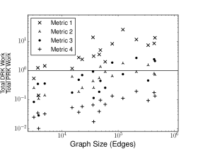
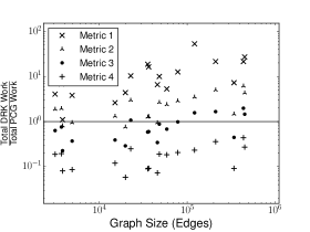
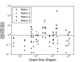
We compare DRK to the other solvers by examining the ratio of DRK work to the work of the other solvers. The ratio of DRK work to PRK work is plotted in Figure 1, separated by graph type. Each vertical set of four points are results for a single graph, and are sorted on the x axis by graph size. The four points represent the ratio of DRK work to PRK work under all four cost metrics. Points above the line indicate DRK performed more work while points below the line indicate DRK performed less work. Similar results for the PCG comparison are shown in Figure 2. Another set of PCG comparisons, converged to the actual error, is shown in Figure 3.
An example of the convergence behavior on the USpowerGrid graph is shown in Figure 4. This plot indicates how both the actual error and relative error behave during the solve for both PCG and DRK. A steeper slope indicates faster convergence. Note this only shows metric 1 work for DRK.
2.3 Experimental Analysis
In the comparison to PRK (shown in Figure 1), DRK is often better with cost metrics 3 and 4. On a few graphs, mostly in the irregular category, DRK outperforms PRK in all cost metrics (all the points are below the line.) In the comparison to PCG (shown in Figure 2), DRK fares slightly better for the irregular graphs, but on both graph sets these results are somewhat less than promising. PCG often does better (most of the points are above the line). Even if we assume unit cost for cycle updates, PCG outperforms DRK. The performance ratios also seem to get worse as graphs get larger.
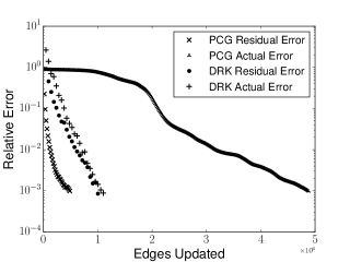
The results concerning the actual error (shown in Figure 3) are very interesting as they are quite different than those with the residual tolerance. For all of the mesh graphs, considering the actual error makes DRK look more promising. The relative performance of cost metrics 3 and 4 are now typically better for DRK than PCG. However, PCG is still consistently better with cost metrics 1 and 2. For some of the irregular graphs, the convergence behavior is similar, but for others things look much better when considering actual error. Informally the number of edges updated by DRK did not change much when switching convergence criteria, but PCG work often increased. The USpowerGrid example (shown in Figure 4) gives a sense of this. The residual error and actual error decrease similarly for DRK, but the actual error curve for PCG decreases much more slowly for the actual error.
3 New Algorithmic Ideas
We consider ways in which DRK could be improved by altering the choice of cycles and their updates. Our goals are both to reduce total work and to identity potential parallelism in DRK. To this end we are interested in measuring the number of parallel steps, the longest number of steps a single thread would have to perform before before convergence, maximized over all threads. Parallel steps are measured in terms of the four cost metrics described in section 2. We will also define the span [9], or critical path length, which is the number of parallel steps with unbounded threads.
3.1 Expanding the Set of Cycles
Sampling fundamental cycles with respect to a tree may require updating several long cycles which will not be edge-disjoint. It would be preferable to update edge-disjoint cycles, as these updates could be done in parallel. The cycle set we use does not need to be a basis, but it does need to span the cycle space. In addition to using a cycle basis from a spanning tree, we will use several small, edge-disjoint cycles. We expect that having threads update these small cycles is preferable to having them stand idle.
3.1.1 2D Grid Example
A simple example of a different cycle basis is the 2D grid graph, shown in Figure 5. In the original DRK, cycles are selected by adding off-tree edges to the spanning tree as in Figure 5(a). As the 2D grid graph is planar, the faces of the grid are the regions bounded by edges, and we refer to the cycles that enclose these regions as facial cycles. We consider using these cycles to perform updates of DRK, as the facial cycles span the cycle space of a planar graph [11]. Half of these cycles can be updated at one iteration and then the other half can be updated during the next iteration, in a checkerboard fashion, as in Figures 5(b)(c). Furthermore, to speed up convergence, smaller cycles can be added together to form larger cycles (in a multilevel fashion) as in Figure 5(d).


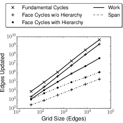
We implemented such a cycle update scheme using the grid facial cycles, and performed experiments to see how the facial cycles affected the total work measured in both the number of cycles updated (metric 4) and edges updated (metric 1). With the facial cycles, the span per iteration is the cost of updating two cycles at each level. We ran experiments with and without the hierarchical combination of the facial cycles against the original set of fundamental cycles. In the case of the fundamental cycles we use H trees [3], which have optimal stretch . Solutions were calculated to a residual tolerance of . The accuracy here is slightly better than the rest of the experiments since these experiments were faster.
The results shown in Figure 6 indicate that the facial cycles improve both the work and span. Using a hierarchical update scheme reduces the total number of edges updated. However as this requires updating larger cycles it has a worse span than simply using the lowest level of cycles.
3.1.2 Extension to General Graphs
We refer to small cycles we add to the basis as local greedy cycles. Pseudocode for finding these cycles is shown in Algorithm 1. We construct this cycle set by attempting to find a small cycle containing each edge using a truncated breadth-first search (BFS). Starting with all edges unmarked, the algorithm selects an unmarked edge and attempts to find a path between its endpoints. This search is truncated by bounding the number of edges searched so that each search is constant work and constructing the entire set is work. If found, this path plus the edge forms a cycle, which is added to the new cycle set, and all edges used are marked. Table 1 shows the number of local greedy cycles found for all the test graphs when the truncated BFS was allowed to search 20 edges. Greedy cycles were found in all the graphs except for tube1, all of whose vertices had such high degree that searching 20 edges was not enough to find a cycle.
Adding additional cycles to the cycle basis means we need new probabilities with which to sample all the cycles. Since in the unweighted case, the stretch of a cycle is just its total length, it seems natural to update cycles proportional to their length.


3.2 Cycle Sampling and Updating in Parallel
In the original DRK algorithm, cycles are chosen one at a time with probability proportional to stretch. We propose a parallel update scheme in which multiple threads each select a cycle, at every iteration, with probability proportional to cycle length. If two threads select cycles that share an edge, one of the threads goes idle for that iteration. In Figure 8, threads 1, 2, and 4 select edge-disjoint cycles. However the third processor selects a cycle which contains edge 3, which is already in use by the cycle on thread 1. Processor 3 sits this iteration out while the other processors update their cycles.

We compute several measures of parallel performance. The first is simply the number of iterations. The second is the total work across all threads at every iteration. Lastly we measure the span, or critical path length. This is the maximum of the work over all threads, summed over all the iterations.
We envision threads working in a shared memory environment on a graph that fits in memory. This might not be realistic in practice as there must be some communication of which edges have already been used which might be too expensive relative to the cost of a cycle update. However we are simply interested in measuring the potential parallelism, thus we ignore any communication cost.
The parallel selection scheme conditions the probabilities with which cycles are selected on edges being available
This scheme creates a bias towards smaller cycles with less conflicting edges as more threads are added, which can increase total work.
4 Experiments and Results
4.1 Experimental Design
We performed experiments on a variety of unweighted graphs from the UF Sparse Matrix Collection (the same set as in Section 2, shown in Table 1). Again we distinguish between mesh-like graphs and irregular graphs. We also use a small test set for weak scaling experiments, consisting of 2D grids and BTER graphs.
We continue to use our Python/Cython implementation of DRK, without a guaranteed low stretch spanning tree or a cycle update data structure. The code does not run in parallel, but we simulate parallelism on multiple threads by selecting and updating edge-disjoint cycles at every iteration as described above.
Our experiments consist of two sets of strong scaling experiments, the spanning tree cycles with and without local greedy cycles, up to 32 threads. We set a relative residual tolerance of . Again we sacrifice accuracy to run more experiments on larger graphs. We consider the same four cycle update cost metrics as in Section 2: cycle length, , , and unit cost update. However in the case of the local greedy cycles, which cannot use the update data structure, we always just charge the number of edges in a cycle. For all the cost models, we measure the total work required for convergence and the number of parallel steps taken to converge. For metric 4 these will be the same. A condensed subset of the scaling results is shown in Table 2.
4.2 Experimental Results
We first examine the effects of using an expanded cycle set in the sequential algorithm. We estimate the usefulness of extra cycles as the length of the largest cycle in the fundamental set normalized by the number of cycles in the fundamental set. This is because we suspect the large cycles to be a barrier to performance, as they are updated the most frequently, and at the highest cost. We plot the performance of the local greedy cycles for the two different graph types, using metrics 1 and 4 in Figure 9). These plots show the ratio between the work of the expanded cycle sets as a function of the estimated usefulness. Points below the line indicate that adding local greedy cycles improved performance.
We examine how the local greedy cycles perform as graph size increases with weak scaling experiments on 2D grid graphs and BTER graphs. The 2D grids used for this experiment are the same as in Figure 6, and the BTER graphs were generated with the parameters: average degree of 20, maximum degree of , global clustering coefficient of 0.15, and maximum clustering coefficient of 0.15. We plot the performance of cost Metric 1 as graph size scales in Figure 10.


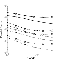
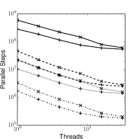
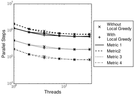
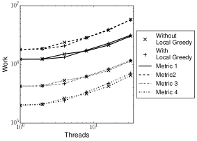
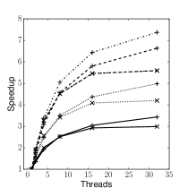
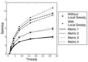

Figure 11 shows examples of our results on three of the graphs. In Figure 11(a) the parallel steps (with the four different metrics) is plotted as a function of the number of threads used for the barth5 graph. The total edges (metric 1) is at the top of the plot, while the unit cost (metric 4) is at the bottom. These results are shown for both fundamental and extended cycle sets. Figure 12 shows the effect of adding threads to the total work.
To measure the parallel performance across multiple graphs we look at the average speedup of the parallel steps across all graphs. Speedup is defined as the sequential work using one thread over the number of parallel steps using a number of multiple threads. The speedup with and without extended cycles is shown in Figure 13. Note that without local greedy cycles metric 2 and metric 4 speedup are the same as the costs differ by . We compare the speedup between the different cycle sets for the different graph types in Figure 14. Results are shown only for metric 1. The speedup of using 8 threads without local greedy is plotted against the speedup of using 8 threads with local greedy.
4.3 Experimental Analysis
In the sequential results shown in Figure 9, there seems to be a threshold of largest cycle length above which local greedy cycles can be useful, but below which there is not much difference. However, there is not a clear scaling with the cycle length ratio, indicating that this is still a crude guess as to where the extended cycle set is useful. Also note that mesh-like graphs tend to have larger girth (max cycle length) than irregular graphs, leading to local greedy cycles working better on meshes. The local greedy cycle improvement is slightly better for metric 1 where we count every edge update. At the other extreme, when updating large cycles is the same cost (unit) as small cycles added by local greedy, the local cycles are less effective. However there is still an improvement in number of cycles updated. We were unable to find some measure of the usefulness of a single local greedy cycle.
The weak scaling experiments shown in Figure 10 show that, with the exception of a BTER outlier, the work scales nicely with graph size. Also results for both cycle sets scale similarly. The extended cycle set benefits the 2D grid graphs while the BTER graphs see little improvement or are worse. This is consistent with Figure 9 since the BTER graphs are irregular and the 2D grids are mesh-like.
The scaling of parallel steps plots show a variety of different behavior on the example graphs. On the mesh-like barth5 graph (shown in Figure 11(a)), the local greedy cycles improve both sequential performance and the scaling of parallel steps performance. At the left of this plot we see the extra cycles improve sequential results. Then as threads are added in parallel, the steeper slope indicates the local greedy cycles improved the scaling of the parallel steps. On the tuma1 graph (shown in Figure 11(b)), the local greedy cycles improve sequential performance, but result in similar or worse scaling. At the left of this plot we see the extra cycles improve results sequentially, but when scaled to 32 threads performance is similar. On the email graph (shown in Figure 11(c)), the local greedy cycles do not improve sequential performance, and scaling is poor with both cycle sets. There is little difference between the different cycle sets in this plot. Furthermore scaling is poor and quickly flattens out by about four threads. For a better understanding of the poor parallel steps scaling on the email graph, we examine the total work scaling (shown in Figure 12), showing how much extra work we have to do when skewing the probability distribution. This extra work quickly increases, limiting the parallel performance.
In the average parallel steps speedup plot (shown in Figure 13), we see similar speedup for both cycle sets. On mesh-like graphs the local greedy cycles do slightly better on all cost metrics beyond 16 threads. However on the irregular graphs, only with cycle cost metric 4 do the local greedy cycles perform better, and under metric 3 they perform worse. (Again note that without local greedy cycles metric 4 and metric 3 speedups are the same.) We hypothesized that giving the solver smaller, extra cycles would improve the parallel performance compared to the fundamental cycles. However this seems to only be true for mesh-like graphs, and even then the improvement is minimal. An interesting thing to note is that the speedup is better with the cost model. This is probably due to overcharging small cycles, which is less problematic when there are more threads to pick potentially larger cycles.
Taking a snapshot of the parallel steps speedup results on eight threads (shown in Figure 14), we see that there are some irregular graphs which do not have much speedup for either cycle set (bottom left of the plot). However there are mesh-like and irregular graphs which enjoy a speedup for both cycle sets (top right of the plot). It is difficult to say on which graphs will different cycles aid with parallelism.
5 Conclusions
We have done an initial comparison of Kelner et al.’s DRK algorithm with PCG and PRK. These preliminary results, measuring algorithm work by number of edges touched or by number of cycles updated, do not at present support the practical utility of DRK. For mesh-like graphs, PCG usually takes less work than DRK, even if DRK is charged only one unit of work per cycle update. This suggests that the fast cycle update data structure proposed by Kelner et al. (or any undiscovered fast update method) will not be enough to make DRK practical. It does seem that DRK is an improvement to PRK on several graphs, mostly irregular graphs. One promising result of these experiments is that DRK converges to small actual error similarly to residual error, while PCG sometimes does not. More PCG iterations are required when solving to a low actual error, while DRK work does not increase very much. More work should be done to understand this behavior.
The experiments in this paper were limited to unweighted graphs for simplicity. Experiments with weighted graphs should be run for more complete results. An open question is whether there is a class of graphs with high condition number, but with practical low stretch trees, where DRK will perform significantly better in practice.
We suggest techniques for improving DRK in practice. We consider using a spanning set, including non-fundamental cycles, to accelerate convergence. Using facial cycles of a two-dimensional grid graph greatly reduces the required number of edge updates compared to the fundamental cycle basis. We attempt to generalize these cycles by finding small local greedy cycles. We found these cycles can accelerate convergence, especially for mesh-like graphs. It is difficult to measure the usefulness of any one cycle in the basis, so it is difficult to determine where and which extra cycles are useful.
We also consider how DRK could be implemented in parallel to take advantage of simultaneous updates of edge disjoint cycles. We describe a model in which threads select cycles, and go idle if a conflicting edge is found. While this can increase total work, it can often reduce the number of parallel steps. However there is a limit to this parallelism. Furthermore, this scaling behavior seems to be similar with or without local greedy cycles.
References
- [1] I. Abraham and O. Neiman. Using petal-decompositions to build a low stretch spanning tree. In Proceedings of the 45th annual ACM Symp. on Theory of Comp., pages 395–406. ACM, 2012.
- [2] R. Agaev and P. Chebotarev. On the spectra of nonsymmetric laplacian matrices. Linear Algebra and its Applications, 399:157–168, 2005.
- [3] N. Alon, R. M. Karp, D. Peleg, and D. West. A graph-theoretic game and its application to the k-server problem. SIAM Journal on Computing, 24(1):78–100, 1995.
- [4] M. Bern, J. Gilbert, B. Hendrickson, N. Nguyen, and S. Toledo. Support-graph preconditioners. SIAM Journal Matrix Anal. Appl., 27(4):930–951, 2006.
- [5] E. G. Boman, D. Chen, B. Hendrickson, and S. Toledo. Maximum-weight-basis preconditioners. Numerical Linear Algebra Appl., 11:695–721, 2004.
- [6] E. G. Boman, B. Hendrickson, and S. Vavasis. Solving elliptic finite element systems in near-linear time with support preconditioners. SIAM Journal on Numerical Anal., 46(6):3264–3284, 2008.
- [7] D. Chen and S. Toledo. Vaidya’s preconditioners: Implementation and experimental study. ETNA. Electronic Transactions on Numerical Analysis [electronic only], 16:30–49, 2003.
- [8] P. Christiano, J. A. Kelner, A. Madry, D. A. Spielman, and S.-H. Teng. Electrical flows, laplacian systems, and faster approximation of maximum flow in undirected graphs. In Proceedings of the 43rd ACM Symp. Theory of Comp. (STOC ’11), pages 273–282. ACM, 2011.
- [9] T. H. Cormen, C. E. Leiserson, R. L. Rivest, and C. Stein. Introduction to Algorithms, pages 779–784. MIT Press and McGraw-Hill, 2009.
- [10] T. A. Davis and Y. Hu. The University of Florida Sparse Matrix Collection. ACM Transactions on Mathematical Software, 38(1):1:1–1:25, Nov. 2011.
- [11] R. Diestel. Graph Theory, volume 173, pages 23–28. Springer, 2012.
- [12] L. Grady. Random walks for image segmentation. IEEE Transactions on Pattern Analysis and Machine Intelligence, 28(11):1768–1783, 2006.
- [13] K. Gremban. Combinatorial Preconditioners for Sparse, Symmetric, Diagonally Dominant Linear Systems. PhD thesis, Carnegie Mellon University, Pittsburgh, October 1996.
- [14] D. Hoske, D. Lukarski, H. Meyerhenke, and M. Wegner. Is nearly-linear the same in theory and practice? A case study with a combinatorial Laplacian solver. Computing Research Repository, abs/1502.07888, 2015.
- [15] S. Kaczmarz. Angenäherte auflösung von systemen linearer gleichungen. Bulletin International de l’Academie Polonaise des Sciences et des Lettres, 35:355–357, 1937.
- [16] J. A. Kelner, L. Orecchia, A. Sidford, and Z. A. Zhu. A simple, combinatorial algorithm for solving SDD systems in nearly-linear time. In Proceedings of the 45th ACM Symp. Theory of Comp. (STOC ’13), pages 911–920, New York, 2013.
- [17] N. L. D. Khoa and S. Chawla. A scalable approach to spectral clustering with sdd solvers. Journal of Intelligent Info. Sys., 44(2):289–308, 2015.
- [18] T. G. Kolda, A. Pinar, T. Plantenga, and C. Seshadhri. A scalable generative graph model with community structure. SIAM Journal on Scientific Comp., 36(5):C424–C452, 2014.
- [19] I. Koutis, G. L. Miller, and R. Peng. Approaching optimality for solving SDD systems. Computing Research Repository, abs/1003.2958, 2010.
- [20] I. Koutis, G. L. Miller, and D. Tolliver. Combinatorial preconditioners and multilevel solvers for problems in computer vision and image processing. Computer Vision and Image Understanding, 115(12):1638 – 1646, 2011.
- [21] O. E. Livne and A. Brandt. Lean algebraic multigrid (LAMG): Fast graph Laplacian linear solver. SIAM Journal on Scientific Comp., 34(4):B499–B522, 2012.
- [22] J. McCann and N. S. Pollard. Real-time gradient-domain painting. ACM Transactions on Graphics, 27(3):93, 2008.
- [23] P. A. Papp. Low-stretch spanning trees. Undergraduate thesis, Eötvös Loránd University, 2014.
- [24] D. A. Spielman and N. Srivastava. Graph sparsification by effective resistances. SIAM Journal on Computing, 40(6):1913–1926, 2011.
- [25] D. A. Spielman and S. Teng. Nearly-linear time algorithms for graph partitioning, graph sparsification, and solving linear systems. In Proceedings of the 36th Annual ACM Symp. on Theory of Comp., STOC ’04, pages 81–90, New York, NY, USA, 2004. ACM.
- [26] T. Strohmer and R. Vershynin. A randomized Kaczmarz algorithm with exponential convergence. Journal of Fourier Analysis and Applications, 15(2):262–278, 2009.
- [27] Z. A. Zhu, S. Lattanzi, and V. S. Mirrokni. A local algorithm for finding well-connected clusters. Computing Research Repository, abs/1304.8132, 2013.
| Graph | Nodes | Edges | 2-core | 2-Core | Greedy | Probability of | Largest |
| (Collection) | Nodes | Edges | Cycles | Selecting Greedy | Cycle Length | ||
| jagmesh3 (HB) | 1.09k | 3.14k | 1.09k | 3.14k | 1.92k | 0.2419 | 77 |
| lshp1270 (HB) | 1.27k | 3.70k | 1.27k | 3.70k | 2.17k | 0.4712 | 95 |
| rail_1357 | 1.36k | 3.81k | 1.36k | 3.81k | 1.85k | 0.2507 | 55 |
| (Oberwolfach) | |||||||
| 50 x 50 grid | 2.50k | 4.90k | 2.50k | 4.90k | 2.40k | 0.5000 | 120 |
| data (DIMACS10) | 2.85k | 15.1k | 2.85k | 15.1k | 7.43k | 0.1760 | 92 |
| 100 x 100 grid | 10.0k | 19.8k | 10.0k | 19.8k | 9.80k | 0.5000 | 230 |
| 20 x 20 x 20 grid | 8.00k | 22.8k | 8.00k | 22.8k | 3.57k | 0.1941 | 122 |
| L-9 (A-G Monien) | 18.0k | 35.6k | 18.0k | 35.6k | 17.6k | 0.4992 | 411 |
| tuma1 | 23.0k | 37.2k | 22.2k | 36.5k | 10.7k | 0.0610 | 420 |
| (GHS_indef) | |||||||
| barth5 (Pothen) | 15.6k | 45.9k | 15.6k | 45.9k | 29.9k | 0.1765 | 375 |
| cti (DIMACS10) | 16.8k | 48.2k | 16.8k | 48.2k | 7.27k | 0.0501 | 172 |
| aft01 (Okunbor) | 8.21k | 58.7k | 8.21k | 58.7k | 26.6k | 0.6680 | 105 |
| 30 x 30 x 30 grid | 27.0k | 78.3k | 27.0k | 78.3k | 8.35k | 0.1399 | 202 |
| wing (DIMACS10) | 62.0k | 122k | 62.0k | 122k | 27.9k | 0.0301 | 605 |
| olesnik0 | 88.3k | 342k | 88.3k | 342k | 220k | 0.1327 | 363 |
| (GHS_indef) | |||||||
| tube1 (TKK) | 21.5k | 438k | 21.5k | 438k | 0 | 0.0000 | 102 |
| fe_tooth (DIMACS10) | 78.1k | 453k | 78.1k | 453k | 217k | 0.3673 | 286 |
| dawson5 (GHS_indef) | 51.5k | 480k | 20.2k | 211k | 19.8k | 0.0941 | 165 |
| Graph | Nodes | Edges | 2-core | 2-core | Greedy | Probability of | Largest |
| (Collection) | Nodes | Edges | Cycles | Selecting Greedy | Cycle Length | ||
| EVA (Pajek) | 8.50k | 6.71k | 314 | 492 | 84 | 0.2346 | 18 |
| bcspwr09 (HB) | 1.72k | 2.40k | 1.25k | 1.92k | 651 | 0.3276 | 54 |
| BTER1 | 981 | 4.85k | 940 | 4.82k | 510 | 0.0465 | 18 |
| , | |||||||
| , | |||||||
| USpowerGrid (Pajek) | 4.94k | 6.59k | 3.35k | 5.01k | 1.68k | 0.2997 | 80 |
| email (Arenas) | 1.13k | 5.45k | 978 | 5.30k | 362 | 0.0433 | 11 |
| uk (DIMACS10) | 4.82k | 6.84k | 4.71k | 6.72k | 1.97k | 0.2488 | 211 |
| as-735 (SNAP) | 7.72k | 13.9k | 4.02k | 10.1k | 3.83k | 0.0822 | 9 |
| ca-GrQc (SNAP) | 4.16 | 13.4k | 3.41k | 12.7k | 4.43k | 0.2315 | 22 |
| BTER2 | 4.86k | 25.1k | 4.54k | 24.8k | 2.69k | 0.0468 | 17 |
| , | |||||||
| , | |||||||
| gemat11 (HB) | 4.93k | 33.1k | 4.93k | 33.1k | 9.72k | 0.0011 | 42 |
| BTER3 | 4.94k | 37.5k | 4.66k | 37.2k | 4.79k | 0.0518 | 18 |
| , | |||||||
| , | |||||||
| dictionary28 (Pajek) | 52.7k | 89.0k | 20.9k | 67.1k | 20.2k | 0.1410 | 36 |
| astro-ph (SNAP) | 16.7k | 121k | 11.6k | 111k | 13.2k | 0.0786 | 18 |
| cond-mat-2003 | 31.2k | 125k | 25.2k | 114k | 32.5k | 0.1533 | 23 |
| (Newman) | |||||||
| BTER4 | 999 | 171k | 999 | 171k | 33 | 0.0002 | 7 |
| , | |||||||
| , | |||||||
| HTC_336_4438 (IPSO) | 226k | 339k | 64.1k | 192k | 32.9k | 0.0339 | 990 |
| OPF_10000 (IPSO) | 43.9k | 212k | 42.9k | 211k | 122k | 0.3146 | 53 |
| ga2010 (DIMACS10) | 291k | 709k | 282k | 699k | 315k | 0.1466 | 941 |
| coAuthorsDBLP | 299k | 978k | 255k | 934k | 297k | 0.1524 | 36 |
| (DIMACS10) | |||||||
| citationCiteseer | 268k | 1.16M | 226k | 1.11M | 150k | 0.0484 | 56 |
| (DIMACS10) |
| Graph | Sequential Work | 2 Thread Parallel Steps | 8 Thread Parallel Steps |
| and Metric | (with Local Greedy) | (with Local Greedy) | (with Local Greedy) |
| jagmesh3 (Metric 1) | 2.73M (1.72M) | 2.02M (1.26M) | 1.07M (28.3K) |
| jagmesh3 (Metric 4) | 127K (101K) | 69.7K (51.2K) | 632K (17.4K) |
| lshp1270 (Metric 1) | 6.80M (4.35M) | 4.87M (3.50M) | 3.41M (2.29M) |
| lshp1270 (Metric 4) | 192K (150K) | 104K (85.1K) | 61.0K (41.9K) |
| rail_1357 (Metric 1) | 1.64M (1.26M) | 1.21M (909K) | 653K (550K) |
| rail_1357 (Metric 4) | 119K (114K) | 63.8K (57.0K) | 143K (143K) |
| 50 x 50 grid (Metric 1) | 9.42M (4.32M) | 9.42M (4.43M) | 3.55M (1.50M) |
| 50 x 50 grid (Metric 4) | 213K (125K) | 115K (62.5K) | 45.0K (20.0K) |
| data (Metric 1) | 17.9M (16.4M) | 13.1M (13.1M) | 8.43M (7.41M) |
| data (Metric 4) | 815K (878K) | 416K (470K) | 185K (168K) |
| 100 x 100 grid (Metric 1) | 84.0M (38.1M) | 59.7M (29.1M) | 27.2M (13.1M) |
| 100 x 100 grid (Metric 4) | 1.11M (610K) | 560K (310K) | 180K (90.0K) |
| 20 x 20 x 20 grid (Metric 1) | 64.7M (63.3M) | 45.3M (46.0M) | 30.9M (28.6M) |
| 20 x 20 x 20 grid (Metric 4) | 1.55M (1.61M) | 816K (856K) | 448K (416K) |
| L-9 (Metric 1) | 820M (382M) | 557M (266M) | 346M (124M) |
| L-9 (Metric 4) | 3.92M (2.03M) | 2.07M (1.04M) | 1.10M (396K) |
| tuma1 (Metric 1) | 597M (282M) | 362M (186M) | 147M (75.9M) |
| tuma1 (Metric 4) | 3.36M (1.69M) | 1.60M (845K) | 512K (267K) |
| barth5 (Metric 1) | 282M (149M) | 212M (119M) | 118M (54.9M) |
| barth5 (Metric 4) | 3.11M (1.98M) | 1.61M (1.03M) | 655K (312K) |
| cti (Metric 1) | 204M (195M) | 142M (143M) | 87.7M (103M) |
| cti (Metric 4) | 3.87M (3.89M) | 2.02M (2.09M) | 1.01M (1.20M) |
| aft01 (Metric 1) | 127M (118M) | 90.8M (88.3M) | 45.4M (43.5M) |
| aft01 (Metric 4) | 4.38M (4.32M) | 2.19M (2.22M) | 763k (738k) |
| 30 x 30 x 30 grid (Metric 4) | 401M (394M) | 284M (283M) | 152M (142M) |
| 30 x 30 x 30 grid (Metric 4) | 6.51M (6.62M) | 3.35M (3.40M) | 1.35M (1.27M) |
| wing (Metric 1) | 4.98B (4.16B) | 3.41B (2.99B) | 2.58B (2.08B) |
| wing (Metric 4) | 21.8M (18.8M) | 12.2M (10.8M) | 8.31M (6.70M) |
| olesnik0 (Metric 1) | 2.69B (1.71B) | 1.99B (1.36B) | 978M (630M) |
| olesnik0 (Metric 4) | 33.8M (24.6M) | 16.9M (1.28M) | 5.47M (3.62M) |
| tube1 (Metric 1) | 2.74B (N/A) | 1.98B (N/A) | 1.59B (N/A) |
| tube1 (Metric 4) | 56.1M (N/A) | 32.0M (N/A) | 22.9M (N/A) |
| fe_tooth (Metric 1) | 6.56B (5.76B) | 4.46B (4.09B) | 3.04B (2.87B) |
| fe_tooth (Metric 4) | 65.5M (62.1M) | 34.3M (32.7M) | 19.8M (18.8M) |
| dawson5 (Metric 1) | 1.49B (1.45B) | 1.06B (1.05B) | 650M (658M) |
| dawson5 (Metric 4) | 24.9M (24.7M) | 12.8M (12.8M) | 6.11M (6.19M) |
| Graph | Sequential Work | 2 Thread Parallel Steps | 8 Thread Parallel Steps |
| and Metric | (with Local Greedy) | (with Local Greedy) | (with Local Greedy) |
| EVA (Metric 1) | 41.4K (25.1K) | 22.5K (23.8K) | 18.5K (15.1K) |
| EVA (Metric 4) | 6.28K (4.08K) | 2.83K (3.14K) | 1.88K (1.88K) |
| bcspwr09 (Metric 1) | 308K (242K) | 199K (165K) | 130K (115K) |
| bcspwr09 (Metric 4) | 26.2K (24.9K) | 12.5K (12.5K) | 4.99K (4.99K) |
| BTER1 (Metric 1) | 2.26M (2.25M) | 1.78M (1.76M) | 1.59M (1.64M) |
| BTER1 (Metric 4) | 246K (253K) | 243K (253K) | 333K (397K) |
| USpowerGrid (Metric 1) | 1.06M (887K) | 735K (557K) | 297K (279K) |
| USpowerGrid (Metric 4) | 73.8K (77.1K) | 36.9K (33.5K) | 10.1K (10.1K) |
| email (Metric 1) | 1.22M (1.23M) | 871K (862K) | 639K (638K) |
| email (Metric 4) | 199K (204K) | 127K (127K) | 87.0K (87.0K) |
| uk (Metric 1) | 7.30M (3.88M) | 5.51M (3.29M) | 3.04M (1.62M) |
| uk (Metric 4) | 160K (108K) | 84.8K (61.2K) | 33.0K (18.8K) |
| as-735 (Metric 1) | 911K (887K) | 498K (550K) | 293K (267K) |
| as-735 (Metric 4) | 201K (201K) | 96.6K (109K) | 48.3K (44.2K) |
| ca-GrQc (Metric 1) | 2.98M (3.39M) | 1.92M (2.16M) | 923K (950K) |
| ca-GrQc (Metric 4) | 413K (509K) | 201K (242K) | 71.7K (75.1K) |
| BTER2 (Metric 1) | 11.3M (11.7M) | 8.21M (8.31M) | 6.52M (6.60M) |
| BTER2 (Metric 4) | 1.30M (1.39M) | 876K (894K) | 658K (667K) |
| gemat11 (Metric 1) | 63.7M (62.2M) | 50.4M (49.4M) | 45.7M (44.9M) |
| gemat11 (Metric 4) | 3.30M (3.22M) | 2.38M (2.33M) | 2.07M (2.04M) |
| BTER3 (Metric 1) | 18.5M (19.0M) | 14.6M (14.1M) | 13.4M (12.4M) |
| BTER3 (Metric 4) | 2.13M (2.27M) | 1.59M (1.54M) | 1.39M (1.29M) |
| dictionary28 (Metric 1) | 38.0M (33.8M) | 24.4M (24.6M) | 16.4M (15.2M) |
| dictionary28 (Metric 4) | 3.20M (3.18M) | 1.65M (1.78M) | 941K (878K) |
| astro-ph (Metric 1) | 25.3M (25.9M) | 15.7M (16.3M) | 8.63M (8.57M) |
| astro-ph (Metric 4) | 4.45M (4.74M) | 2.27M (2.43M) | 1.01M (1.01M) |
| cond-mat-2003 (Metric 1) | 38.8M (40.9M) | 27.4M (30.3M) | 21.0M (20.5M) |
| cond-mat-2003 (Metric 4) | 4.57M (5.35M) | 2.62M (3.10M) | 1.74M (1.72M) |
| BTER4 (Metric 1) | 25.4M (26.4M) | 15.1M (15.1M) | 8.53M (8.01M) |
| BTER4 (Metric 4) | 6.78M (7.06M) | 3.67M (3.67M) | 1.84M (1.73M) |
| HTC_336_4438 (Metric 1) | 14.2B (13.7B) | 8.50B (8.89B) | 4.10B (3.67B) |
| HTC_336_4438 (Metric 4) | 32.2M (32.0M) | 15.9M (16.9M) | 6.80M (6.09M) |
| OPF_10000 (Metric 1) | 47.3M (49.1M) | 31.8M (33.2M) | 16.0M (16.5M) |
| OPF_10000 (Metric 4) | 6.86M (8.66M) | 3.34M (4.29M) | 857K (1.07M) |
| ga2010 (Metric 1) | 8.77B (6.16B) | 6.88B (4.97B) | 3.21B (2.59B) |
| ga2010 (Metric 4) | 40.8M (33.5M) | 20.8M (16.9M) | 6.48M (5.35B) |
| coAuthorsDBLP (Metric 1) | 539M (552M) | 356M (371M) | 264M (237M) |
| coAuthorsDBLP (Metric 4) | 44.4M (51.3M) | 23.5M (26.3M) | 15.3M (13.8M) |
| citationCiteseer (Metric 1) | 1.08B (1.07B) | 716M (723M) | 506M (482M) |
| citationCiteseer (Metric 4) | 74.4M (76.2M) | 40.7M (41.8M) | 25.3M (24.2M) |