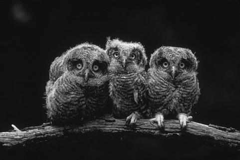
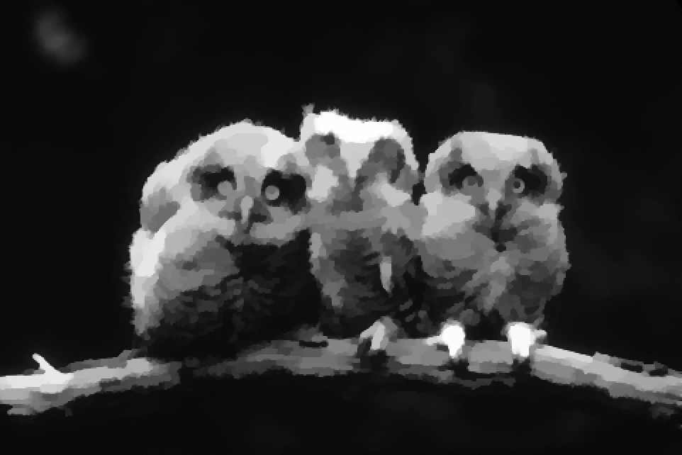
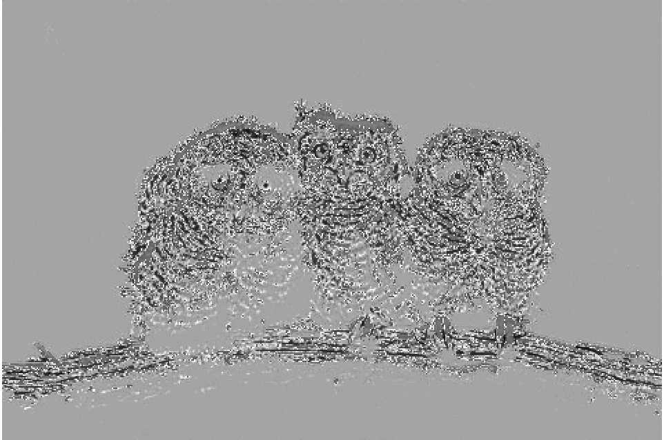
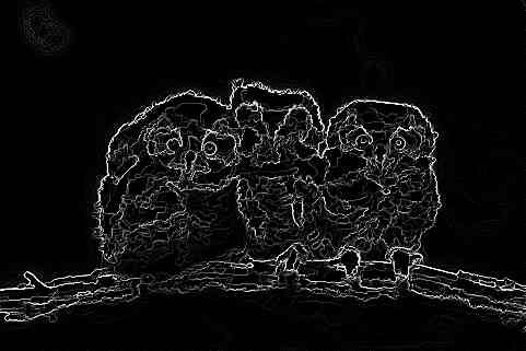
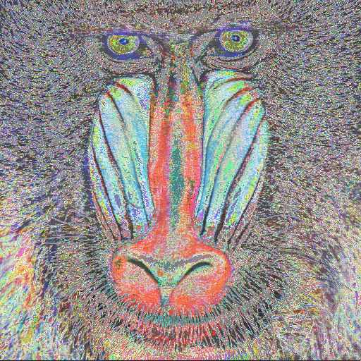
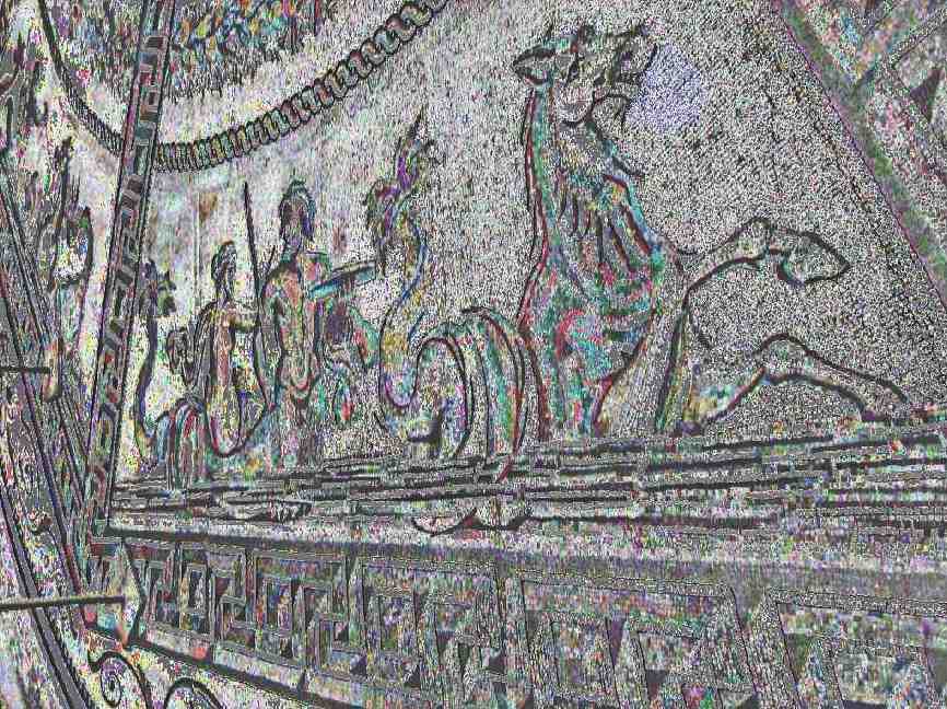
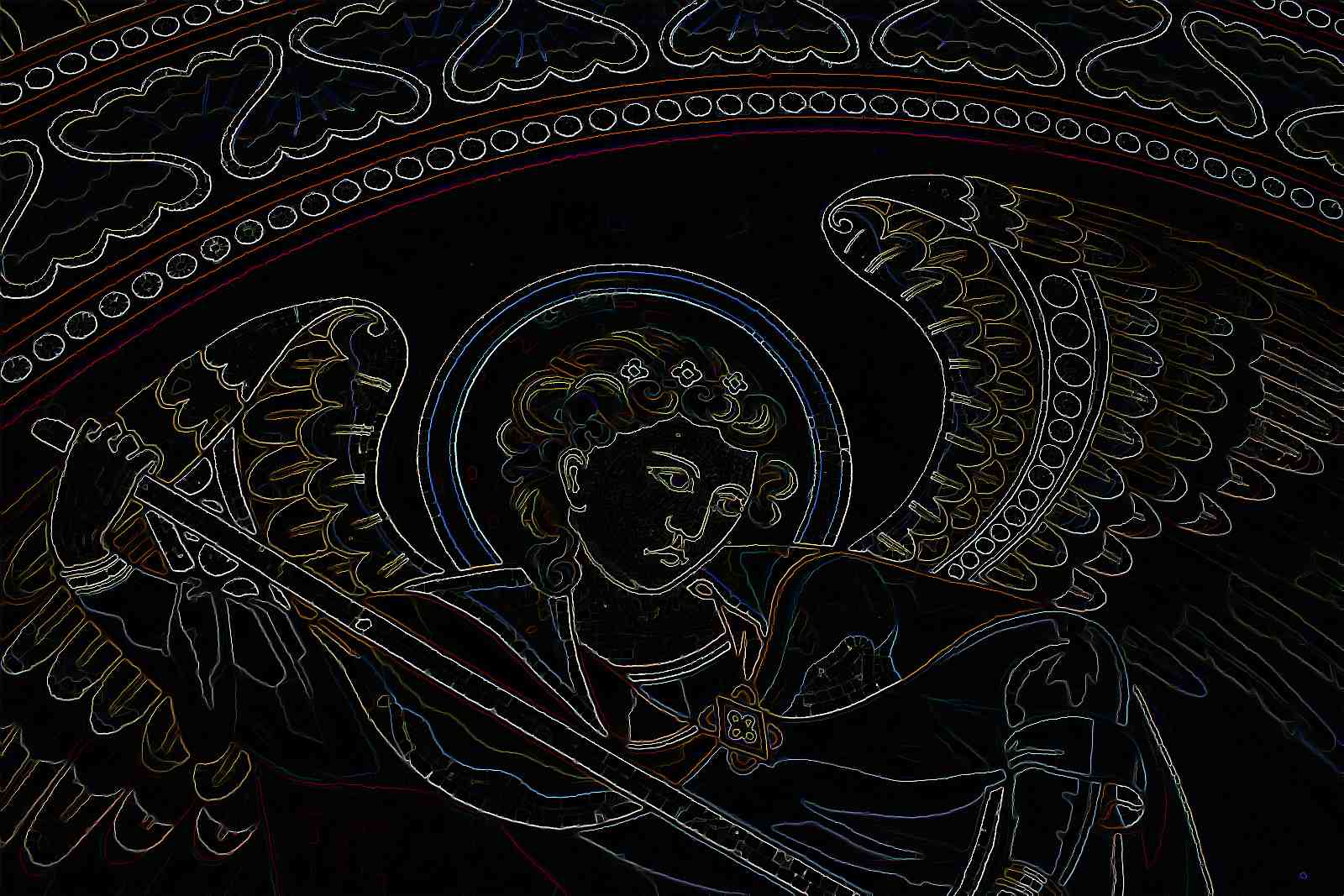
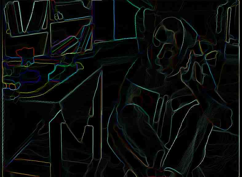
Adaptive diffusion constrained total variation scheme with application to ‘cartoon + texture + edge’ image decompositionthanks: An earlier version available as Preprint Number 13-54, Department of Mathematics, Universidade de Coimbra, Portugal. http://www.mat.uc.pt/preprints/ps/p1354.pdf

Juan C. Moreno Corresponding author. IT, Department of Computer Science, University of Beira Interior, 6201–001, Covilhã, Portugal. E-mail: jmoreno@ubi.pt.    V. B. Surya Prasath Department of Computer Science, University of Missouri-Columbia, MO 65211 USA. E-mail: prasaths@missouri.edu    D. Vorotnikov Department of Mathematics, University of Coimbra, Portugal    Hugo Proença IT, Department of Computer Science, University of Beira Interior, 6201–001, Covilhã, Portugal.    K. Palaniappan Department of Computer Science, University of Missouri-Columbia, MO 65211 USA.
Abstract

We consider an image decomposition model involving a variational (minimization) problem and an evolutionary partial differential equation (PDE). We utilize a linear inhomogenuous diffusion constrained and weighted total variation (TV) scheme for image adaptive decomposition. An adaptive weight along with TV regularization splits a given image into three components representing the geometrical (cartoon), textural (small scale - microtextures), and edges (big scale - macrotextures). We study the wellposedness of the coupled variational-PDE scheme along with an efficient numerical scheme based on Chambolle’s dual minimization [14]. We provide extensive experimental results in cartoon-texture-edges decomposition, and denoising as well compare with other related variational, coupled anisotropic diffusion PDE based methods.

Keywords: Image decomposition, total variation, linear diffusion, adaptive weights, multi-scale, denoising.

1 Introduction

Decomposing an image into meaningful components is an important and challenging inverse problem in image processing. Image denoising is a very well known example of image decomposition. In such a decomposition, the given image is assumed to be under the influence of noise, and the main purpose is to remove noise without destroying edges. This denoising task can be regarded as a decomposition of the image into noise-free signal and noise part. There exist various methodologies for image restoration, where variational minimization and partial differential equation (PDE) are two of the most popular ones [3].

Another important example of image decomposition is based on its smooth and texture components using the total variation (TV) regularization method. This was first studied by Rudin et al [49] for image restoration. The TV regularization can be written as an unconstrained minimization,

minuETV(u)=Ω|u|𝑑x+12αΩ|uf|2𝑑x.subscript𝑢subscript𝐸𝑇𝑉𝑢subscriptΩ𝑢differential-d𝑥12𝛼subscriptΩsuperscript𝑢𝑓2differential-d𝑥\displaystyle\min_{u}E_{TV}(u)=\int_{\Omega}\left|\nabla u\right|\,dx+\frac{1}{2\alpha}\,\int_{\Omega}\left|u-f\right|^{2}\,dx. (1)

The parameter α>0𝛼0\alpha>0 balances the fidelity term with respect to the TV regularization. Let the given image be written as f=u+v𝑓𝑢𝑣f=u+v, where the function u𝑢u models well structured homogeneous regions (cartoon) and v𝑣v defines oscillating patterns such as noise and texture.  [34] established the scale connection property of TV for image decomposition, namely that the α𝛼\alpha parameter is related to the scale of objects in the image. In particular, Meyer proved that if f𝑓f is a characteristic function and is sufficiently small with respect to a norm (|f|1/2αsubscript𝑓12𝛼\left|f\right|_{*}\leq 1/2\alpha), then the minimization of the TV regularization (1) gives u=0𝑢0u=0 and f=0𝑓0f=0, which is counter-intuitive since one expects u=f𝑢𝑓u=f and v=0𝑣0v=0. Thus, Meyer proposed to use dual of the closure in the bounded variation (BV𝐵𝑉BV) space of the Schwartz class for non-trivial solutions, we refer to [34] for more details. This crucial fact has been exploited by [56] to obtain numerical approximations to the Meyer decomposition model, see also related early works [4, 6].

Image denoising methods in general and variational PDE models in particular provide natural decomposition of images, see [3] for a review. Image smoothing and denoising literature is rich in terms of different methodologies utilized and current state of the art techniques [10, 19, 43] have pushed the envelope of optimal improvements [18]. Next we provide a brief overview different approaches utilized in image decomposition.
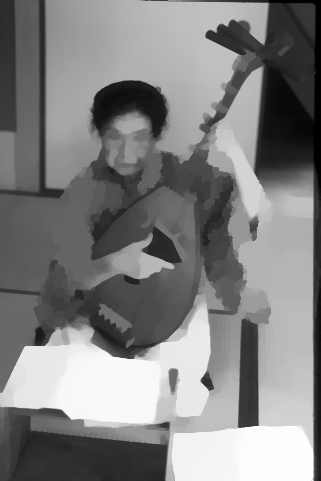
Refer to caption
(a) Input
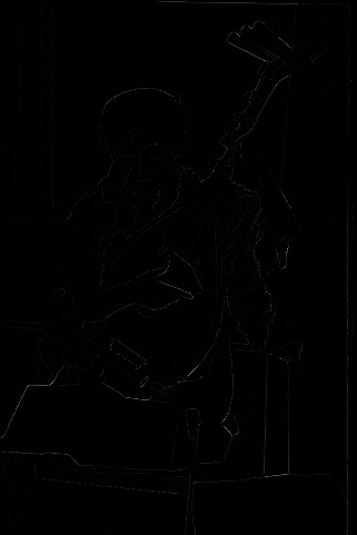
Refer to caption
(b) Cartoon (u𝑢u)
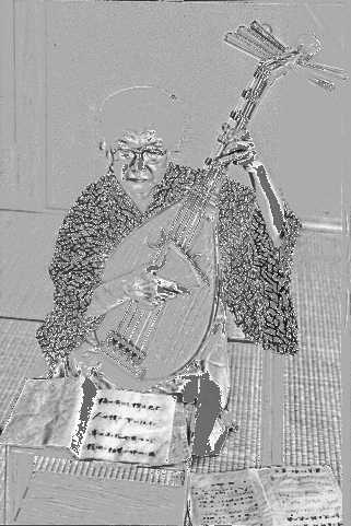
Refer to caption
(c) Texture (v𝑣v)
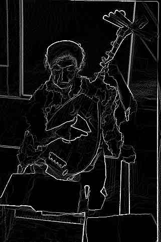
Refer to caption
(d) (Pseudo) Edges (w𝑤w)
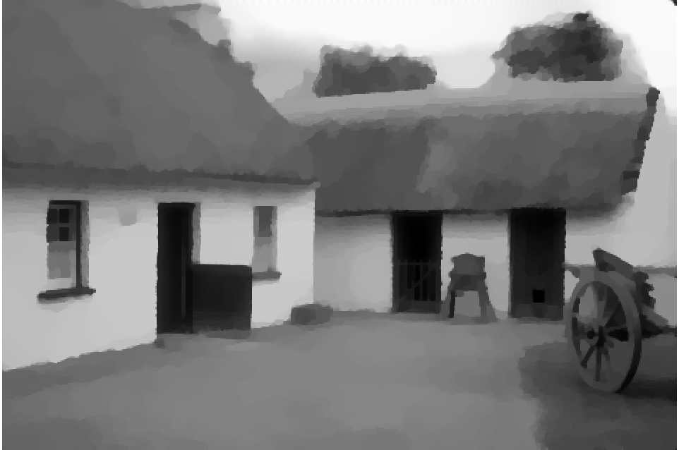
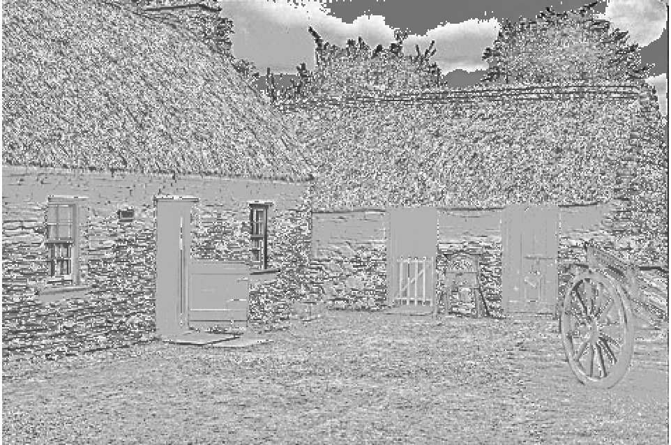
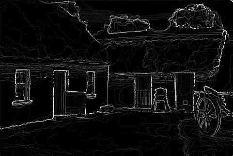
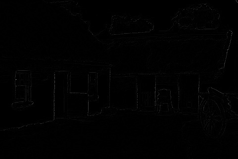
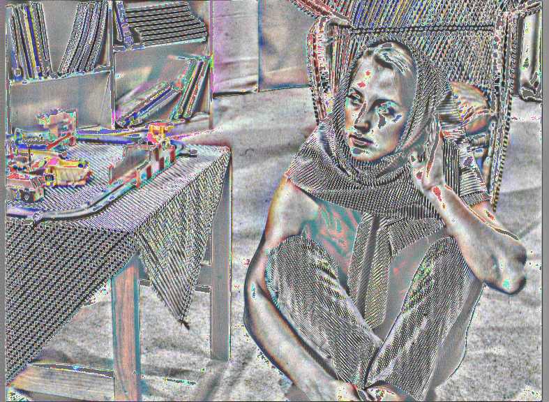
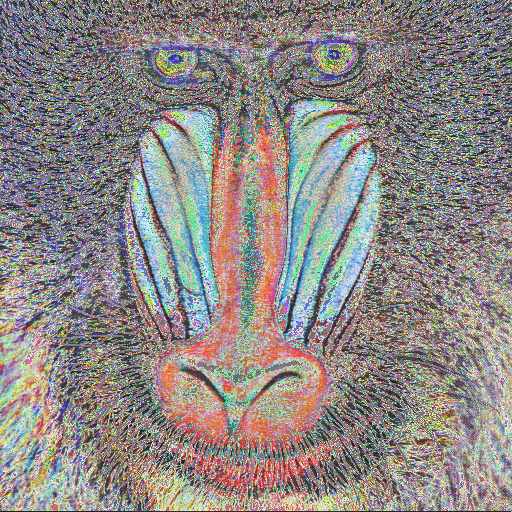
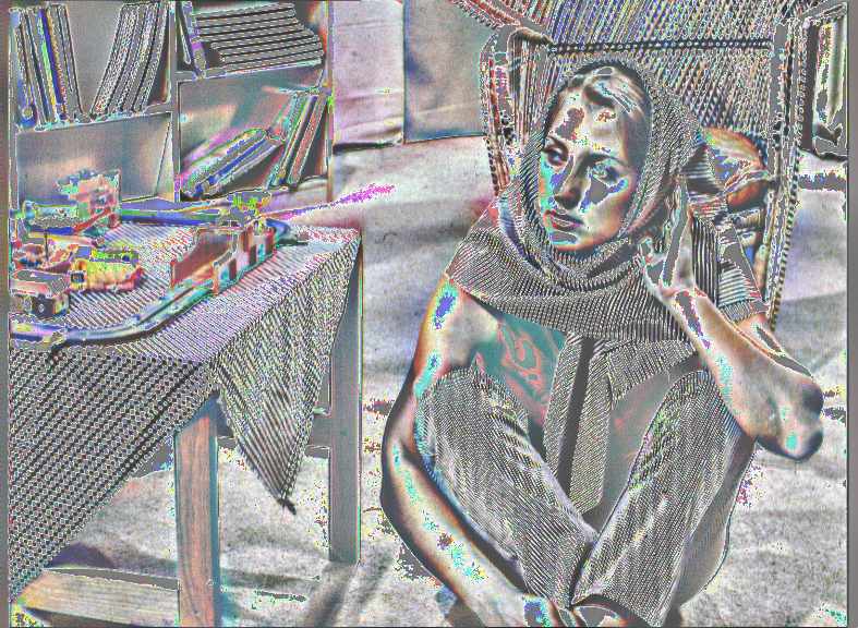
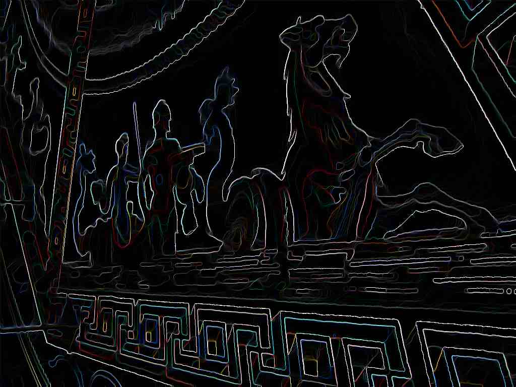
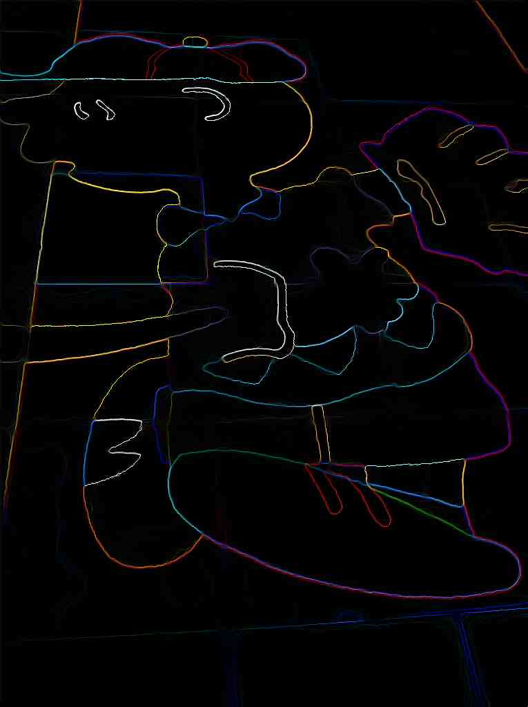
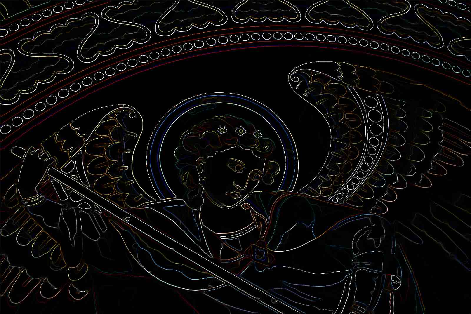
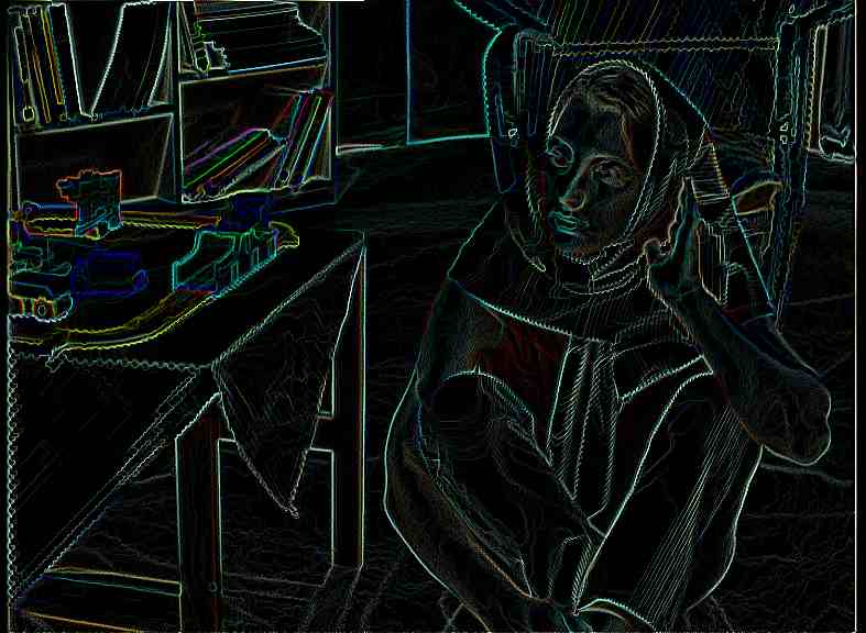
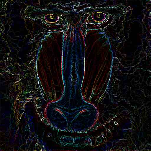
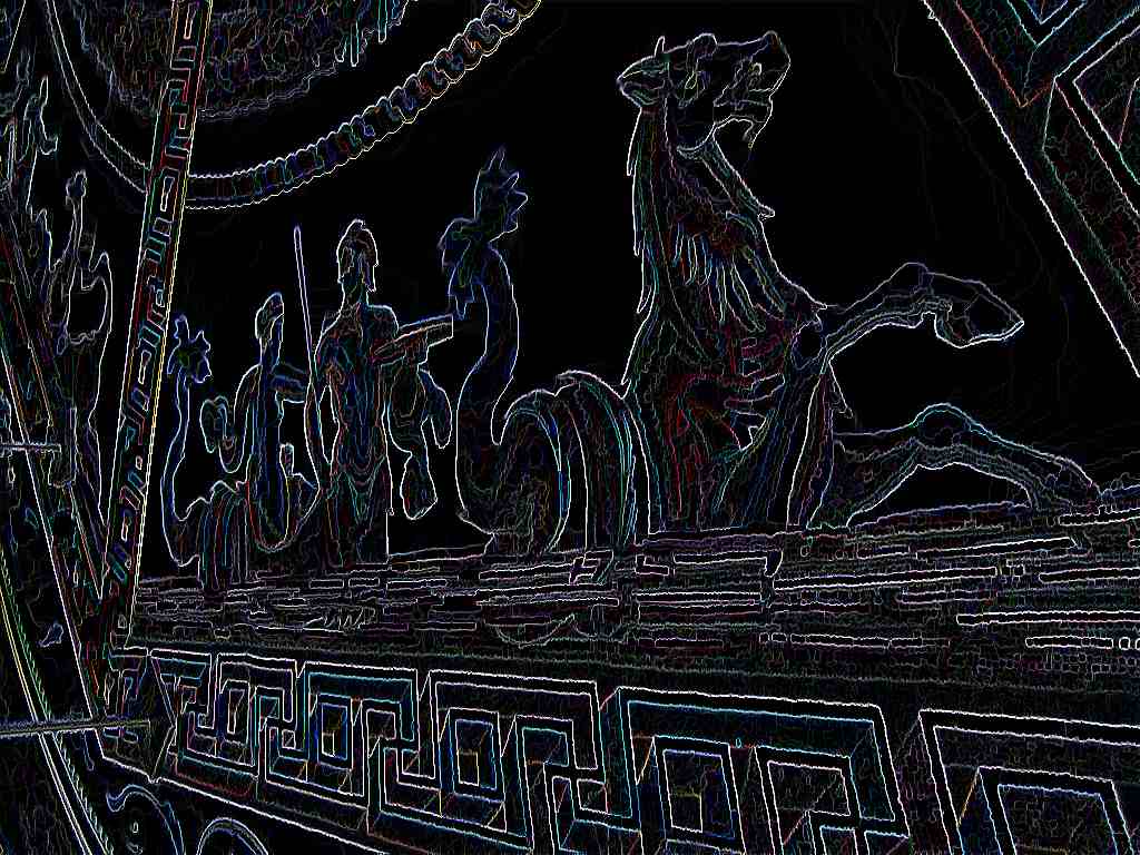
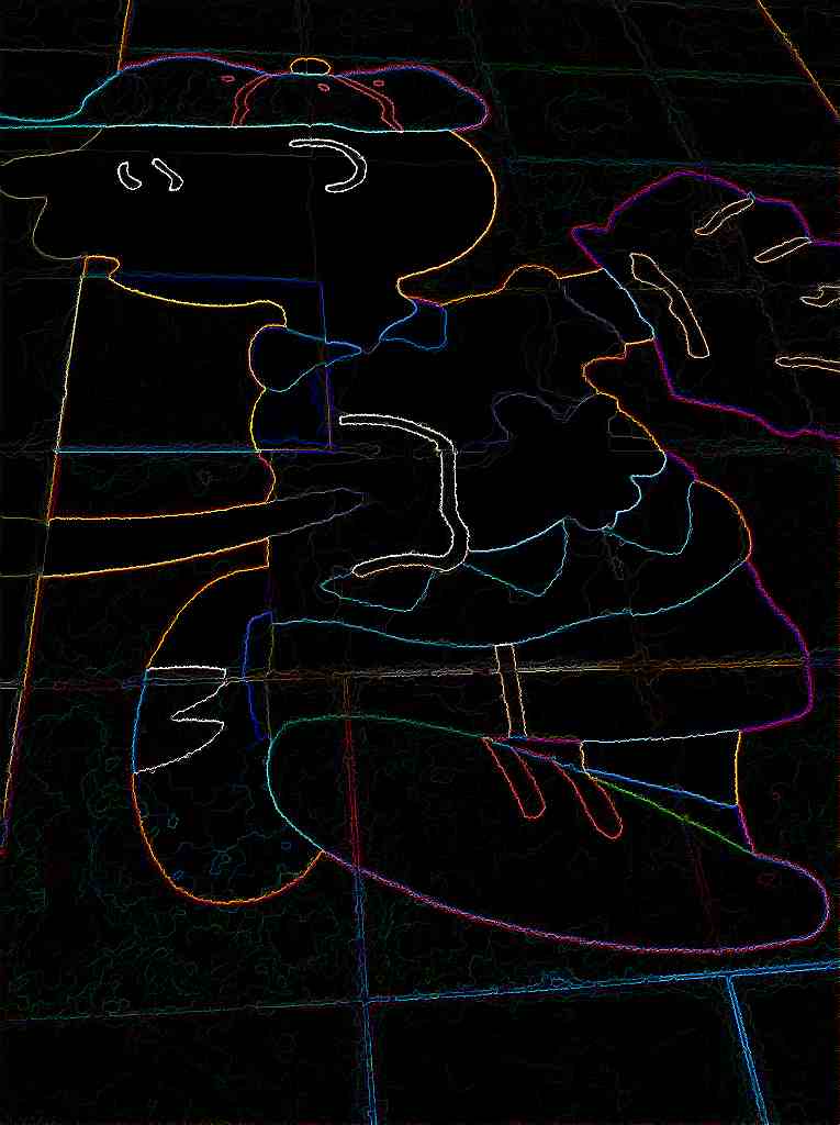
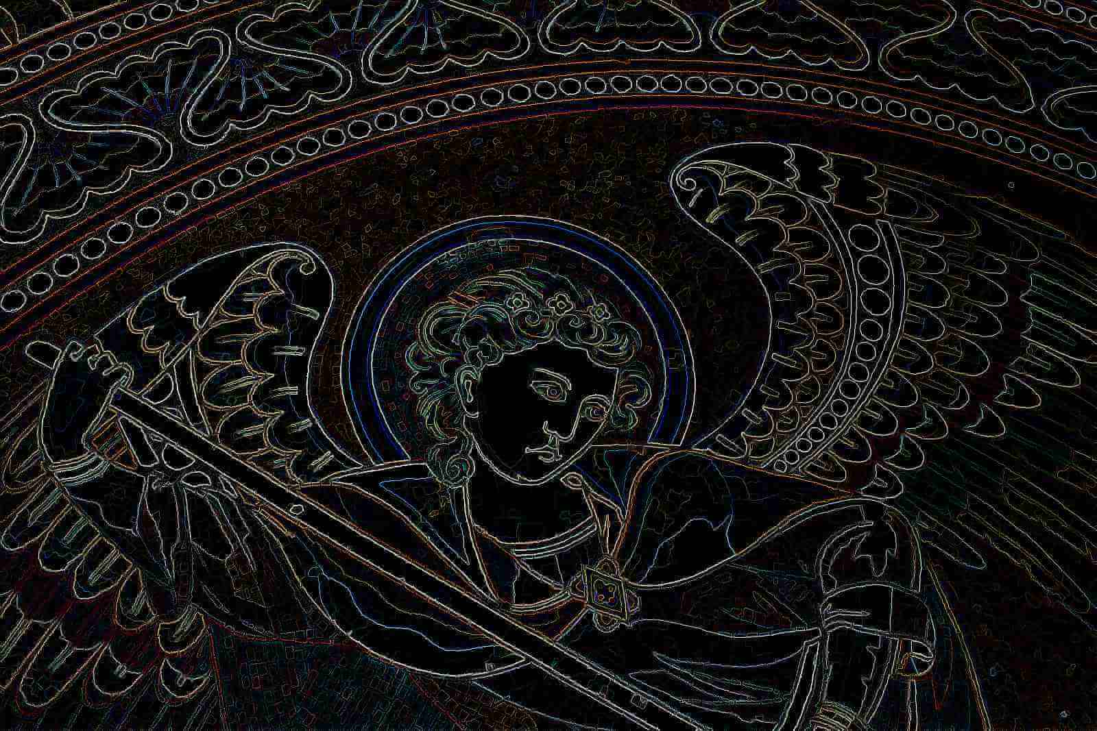
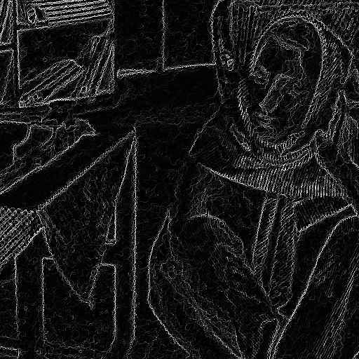
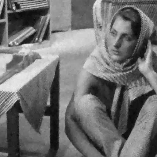
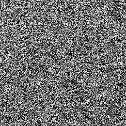
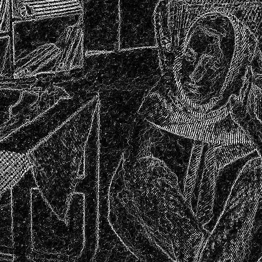
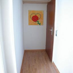
Figure 1: MIT LabelMe decomposition result on an indoor image. Our scheme can obtain piecewise constant cartoon component along with texture and edges for better separation of basic shape elements present in a scene. Better viewed online and zoomed in.

1.1 Literature

While the literature on cartoon and texture decomposition is extensive by now, three lines of inquiries are closely related to the work presented here.

  • Different function spaces for modeling the textures and discrete approximations: Following Meyer’s seminal work [34], various authors have considered different function spaces to model textures accurately [5, 31, 6, 40, 24, 27, 32, 29, 54].

  • L1superscript𝐿1L^{1} fidelity based TV regularization models: In another related direction the fidelity term can be made L1superscript𝐿1L^{1} and is proven to provide contrast preserving restorations. We refer to [16] for the geometric motivation and fine properties of L1superscript𝐿1L^{1} fidelity term, see also [21]. Applications of L1superscript𝐿1L^{1}-TV models for cartoon plus texture decomposition are considered as well [37, 58, 59, 27, 22, 2].

  • Different Regularizers instead of TV: The well-known staircasing property of the TV regularization has been analyzed by many in the past [38, 12, 13] and various modifications have also been studied. To avoid staircasing and blocky restoration results from the classical TV model there have been a variety of methods studied previously. Weighted and adaptive [52, 51, 46, 45, 47], nonlocal-TV [30], and higher order [17, 7, 28, 41].

Out of other related decomposition models we mention multi-scale parameter based models [53, 26, 54] which progressively capture texture. Extension to multichannel images in general, RGB images in particular, is also an important area of research [8]. Note that all of the above mentioned methods obtain cartoon and texture decomposition and in this work we obtain edges as part of our scheme. In Figure 1 we show an example decomposition for an indoor image taken from the MIT LabelMe [50] open annotation. Our advanced decomposition provides basic scene elements, since it is based on total variation (edge preserving) smoothing, the cartoon component reflects coarse shapes. This feature is useful in obtaining segmentations and annotations as the edges can provide guideline for separating salient objects [39].

1.2 Contributions

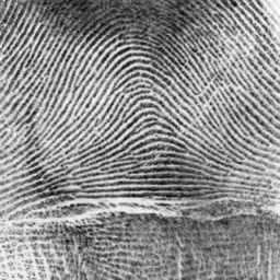
In this paper, we propose a new image decomposition scheme which splits a given image into its geometrical and textural part along with an edge capturing diffusion constraint. Following the success of weighted and adaptive TV models, our scheme is based on a weighted TV regularization where the edge-variable-based weight is computed in a data-adaptive way. The scheme is implemented using the splitting method of [9] along with dual minimization scheme for the weighted TV regularization [14]. As a by-product of the implementation via dual minimization we obtain an auxiliary variable which is akin to textural component of the given image. Thus, the scheme studied here provides a cartoon, texture, edge (CTE) decomposition for digital images, see Figure 2 for some examples111We use the words edges or pseudo-edges interchangeably in the text, since the edge component is computed with gradient maps without traditional edge refinement procedures such as maxima suppression [11]..

We consider the color image decomposition using the dual minimization based color TV model. Multi-scale decomposition following the recent work of [54] is also given. Moreover, we provide theoretical analysis of the model with a priori estimates and prove its solvability. Extensive experimental results on synthetic, textured real images are given. Further, illustrative comparison with other state-of-the-art models are undertaken and the results indicate superior performance of our scheme with respect to cartoon, texture separation as well as denoising with edge preservation.
Refer to caption
Refer to caption
Refer to caption
Refer to caption
Refer to caption
Refer to caption
Refer to caption
Refer to caption
Refer to caption
Refer to caption
Refer to caption
Refer to caption
Refer to caption
Refer to caption
Refer to caption
Refer to caption
Refer to caption
Refer to caption
Refer to caption
Refer to caption
Refer to caption
(a) Input (f𝑓f)
Refer to caption
(b) Cartoon (u𝑢u)
Refer to caption
(c) Texture v𝑣v
Refer to caption
(d) (Pseudo) Edges (w𝑤w)
Refer to caption
(e) f(u+v+w)𝑓𝑢𝑣𝑤f-(u+v+w)
Figure 2: The proposed coupled TV regularization with linear diffusion PDE model provides cartoon, texture and edge decomposition of images (stopping parameter ϵ=104italic-ϵsuperscript104\epsilon=10^{-4}). Better viewed online and zoomed in.

The rest of the paper is organized as follows. Section 2 introduces the adaptive TV regularization coupled with a diffusion PDE. Section 3 provides wellposedness results for our coupled model. In Section 4 we provide the experimental results conducted on real and synthetic images and comparison with related schemes. Finally, Section 5 concludes the paper.

2 Diffusion constrained regularization

2.1 Weighted total variation minimization

The total variation based regularization [49] given in Eqn. (1) is well-known in edge preserving image restoration, we rewrite it as follows,

minuETVμ(u)=Ω|u|𝑑x+μΩ|uf|2𝑑xsubscript𝑢subscriptsuperscript𝐸𝜇𝑇𝑉𝑢subscriptΩ𝑢differential-d𝑥𝜇subscriptΩsuperscript𝑢𝑓2differential-d𝑥\displaystyle\min_{u}E^{\mu}_{TV}(u)=\int_{\Omega}\left|\nabla u\right|\,dx+\mu\,\int_{\Omega}\left|u-f\right|^{2}\,dx (2)

where now μ>0𝜇0\mu>0 is the image fidelity parameter which is important in obtaining results in denoising and cartoon+texture decomposition. A related approach is to consider a weighted total variation,

minuEgTVμ(u)=Ωg(x,u,u)|u|𝑑x+μΩ|uf|2𝑑xsubscript𝑢subscriptsuperscript𝐸𝜇𝑔𝑇𝑉𝑢subscriptΩ𝑔𝑥𝑢𝑢𝑢differential-d𝑥𝜇subscriptΩsuperscript𝑢𝑓2differential-d𝑥\displaystyle\min_{u}E^{\mu}_{gTV}(u)=\int_{\Omega}g(x,u,\nabla u)\left|\nabla u\right|\,dx+\mu\,\int_{\Omega}\left|u-f\right|^{2}\,dx (3)

where g(x,u,u)𝑔𝑥𝑢𝑢g(x,u,\nabla u) represents the generalized weight function. For example,  [9] have considered a convex regularization of the variational model

minu{Ωg(x)|u|𝑑x+μΩ|uf|𝑑x}subscript𝑢subscriptΩ𝑔𝑥𝑢differential-d𝑥𝜇subscriptΩ𝑢𝑓differential-d𝑥\min\limits_{u}\left\{\int_{\Omega}g(x)|\nabla u|\,dx+\mu\int_{\Omega}|u-f|\,dx\right\}

using a fast minimization based on a dual formulation to get a partition in the geometric and texture information. Note that the image fidelity is changed to L1superscript𝐿1L^{1} norm, we refer to [16] for more details. The convex regularization version is considered in [9],

minu,v{Ωg(x)|u|𝑑x+12θΩ(u+vf)2𝑑x+μΩ|v|𝑑x},subscript𝑢𝑣subscriptΩ𝑔𝑥𝑢differential-d𝑥12𝜃subscriptΩsuperscript𝑢𝑣𝑓2differential-d𝑥𝜇subscriptΩ𝑣differential-d𝑥\displaystyle\min\limits_{u,v}\Bigg{\{}\int_{\Omega}g(x)|\nabla u|\,dx+\frac{1}{2\theta}\int_{\Omega}(u+v-f)^{2}\,dx+\mu\int_{\Omega}|v|\,dx\Bigg{\}}, (4)

where the parameter θ>0𝜃0\theta>0 is chosen to be small so that f𝑓f almost satisfies fu+vsimilar-to𝑓𝑢𝑣f\sim u+v, with the function u𝑢u representing geometric information, i.e. the piecewise-smooth regions, and function v𝑣v captures texture information lying in the given image. The function g𝑔g is an edge indicator function that vanishes at object boundaries, for example,

g(x):=11+β|f(x)|2,assign𝑔𝑥11𝛽superscript𝑓𝑥2g(x):=\displaystyle\frac{1}{1+\beta\left|\nabla f(x)\right|^{2}},

where f𝑓f is the original image and β𝛽\beta is an arbitrary positive constant. Thus, we see that TV based minimization models naturally lead to cartoon and texture decomposition of digital images. The image fidelity parameter μ𝜇\mu can be made data adaptive to obtain texture preserving restorations, see [25].

2.2 Description of the model

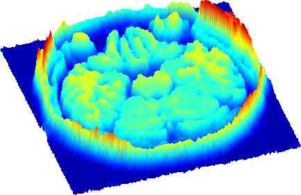
Refer to captionRefer to caption(a) Original Image Refer to captionRefer to captionRefer to captionRefer to caption(b) Cartoon component u with stooping parameters ϵ=104ϵ=105ϵ=106 and ϵ=107 using the proposed model Refer to captionRefer to captionRefer to captionRefer to caption(c) Cartoon component u with stooping parameters ϵ=104ϵ=105ϵ=106 and ϵ=107 using the model in [9]Refer to captionRefer to caption(a) Original Image Refer to captionRefer to captionRefer to captionRefer to caption(b) Cartoon component u with stooping parameters ϵ=104ϵ=105ϵ=106 and ϵ=107 using the proposed model Refer to captionRefer to captionRefer to captionRefer to caption(c) Cartoon component u with stooping parameters ϵ=104ϵ=105ϵ=106 and ϵ=107 using the model in [9]\begin{array}[]{c}\includegraphics[width=68.28644pt]{fig1synthetic_D17D55-icon}\quad\includegraphics[width=85.35826pt]{fig1synthetic_D17D55-icon_surface}\\ \mbox{\scriptsize{(a) Original Image }}\\ \includegraphics[width=85.35826pt]{fig1synthetic_CTE_D17D55-icon_100}\includegraphics[width=85.35826pt]{fig1synthetic_CTE_D17D55-icon_200}\includegraphics[width=85.35826pt]{fig1synthetic_CTE_D17D55-icon_300}\includegraphics[width=85.35826pt]{fig1synthetic_CTE_D17D55-icon_400}\\ \mbox{\scriptsize{(b) Cartoon component $u$ with stooping parameters $\epsilon=10^{-4}$, $\epsilon=10^{-5}$, $\epsilon=10^{-6}$ and $\epsilon=10^{-7}$ using the proposed model }}\\ \includegraphics[width=85.35826pt]{fig1synthetic_Bresson_D17D55-icon_100}\includegraphics[width=85.35826pt]{fig1synthetic_Bresson_D17D55-icon_200}\includegraphics[width=85.35826pt]{fig1synthetic_Bresson_D17D55-icon_300}\includegraphics[width=85.35826pt]{fig1synthetic_Bresson_D17D55-icon_400}\\ \mbox{\scriptsize{(c) Cartoon component $u$ with stooping parameters $\epsilon=10^{-4}$, $\epsilon=10^{-5}$, $\epsilon=10^{-6}$ and $\epsilon=10^{-7}$ using the model in~{}\cite[cite]{[\@@bibref{}{BE07}{}{}]}}}\end{array}
Figure 3: (Color online) Our adaptive diffusion constrained total variation scheme (see Eqn. (9)) with constant μ𝜇\mu, λ𝜆\lambda (second row) provides better edge preserving image decomposition when compared to the traditional TV regularization model (Eqn. (4)) of [9] (third row) as stoping parameters increase from ϵ=104italic-ϵsuperscript104\epsilon=10^{-4} to ϵ=107italic-ϵsuperscript107\epsilon=10^{-7}. The proposed scheme keeps the structure without diffusing its boundary with the background.

In our work, we consider the following regularization model which was motivated by a coupled PDE modeling done in [48] for image restoration,

minu{Ωϕ(x,u,|u|)𝑑x+μΩ|uf|𝑑x},subscript𝑢subscriptΩitalic-ϕ𝑥𝑢𝑢differential-d𝑥𝜇subscriptΩ𝑢𝑓differential-d𝑥\displaystyle\min\limits_{u}\left\{\int_{\Omega}\phi(x,u,|\nabla u|)\,dx+\mu\int_{\Omega}|u-f|\,dx\right\}, (5)
wt=λdiv(w)+(1λ)(|u|w).𝑤𝑡𝜆𝑑𝑖𝑣𝑤1𝜆𝑢𝑤\displaystyle\frac{\partial w}{\partial t}=\lambda div(\nabla w)+(1-\lambda)(|\nabla u|-w). (6)

The choice of regularizer ϕitalic-ϕ\phi depends on an application area and among a plethora of convex and non-convex functions available with the classical TV [49] and the non-local TV [30]. Motivated from the above discussions in Section 2.1, and success enjoyed by the weighted L1superscript𝐿1L^{1}-TV regularization model in image denoising and segmentation, we use L1superscript𝐿1L^{1}-TV regularizer model as a prime example to illustrate our model here. The proposed CTE model thus consists of a minimization along with a non-homogeneous diffusion equation,

minu{Ωg(w)|u|𝑑x+Ωμ(x)|uf|𝑑x},subscript𝑢subscriptΩ𝑔𝑤𝑢differential-d𝑥subscriptΩ𝜇𝑥𝑢𝑓differential-d𝑥\displaystyle\min\limits_{u}\left\{\int_{\Omega}g(w)|\nabla u|\,dx+\int_{\Omega}\mu(x)\,|u-f|\,dx\right\}, (7)
wt=λ(x)div(w)+(1λ(x))(|u|w),𝑤𝑡𝜆𝑥𝑑𝑖𝑣𝑤1𝜆𝑥𝑢𝑤\displaystyle\frac{\partial w}{\partial t}=\lambda(x)div(\nabla w)+(1-\lambda(x))(|\nabla u|-w), (8)

where g(w)=11+w2𝑔𝑤11superscript𝑤2g(w)=\frac{1}{1+w^{2}}, or g(w)=exp(w2)𝑔𝑤𝑒𝑥𝑝superscript𝑤2g(w)=exp(-w^{2}) (Perona-Malik type diffusion functions [42]), or g(w)=|w|1𝑔𝑤superscript𝑤1g(w)=\left|w\right|^{-1}, or g(w)=1ϵ2+|w|2𝑔𝑤1superscriptitalic-ϵ2superscript𝑤2g(w)=\frac{1}{\sqrt{\epsilon^{2}+\left|w\right|^{2}}} (total variation diffusion function [49]). That is we solve adaptive data fidelity based weighted total variation minimization for the smooth part u𝑢u using Eqn. (7) along with a linear non-homogenous diffusion constraint on w𝑤w by solving Eqn. (8). Note that the balancing parameter λ𝜆\lambda and image fidelity μ𝜇\mu taking values in [0,1]01[0,1] are important in our experimental results. Adaptive ways of choosing these parameters are explained below in Section 2.3. Following [9] we use a splitting with an auxiliary variable v𝑣v to obtain

minu,v{Ωg(w)|u|𝑑x+12θΩ(u+vf)2𝑑x+Ωμ(x)|v|𝑑x},subscript𝑢𝑣subscriptΩ𝑔𝑤𝑢differential-d𝑥12𝜃subscriptΩsuperscript𝑢𝑣𝑓2differential-d𝑥subscriptΩ𝜇𝑥𝑣differential-d𝑥\displaystyle\min\limits_{u,v}\Bigg{\{}\int_{\Omega}g(w)|\nabla u|\,dx+\frac{1}{2\theta}\int_{\Omega}(u+v-f)^{2}\,dx+\int_{\Omega}\mu(x)|v|\,dx\Bigg{\}}, (9)
wt=λ(x)div(w)+(1λ(x))(|u|w).𝑤𝑡𝜆𝑥𝑑𝑖𝑣𝑤1𝜆𝑥𝑢𝑤\displaystyle\frac{\partial w}{\partial t}=\lambda(x)div(\nabla w)+(1-\lambda(x))(|\nabla u|-w).

Thus, the computed solution of these equations provides a representation (u,v,w)𝑢𝑣𝑤(u,v,w), where the function u𝑢u represents the geometric information, the function v𝑣v captures the texture information, and the function w𝑤w represents the edges lying in the given image. Figure 3 shows a comparison of our scheme (μ=1𝜇1\mu=1 and λ=0.5𝜆0.5\lambda=0.5) and Bresson et al [9] scheme Eqn. (4) for a synthetic texture image which contains two different texture patterns. As can be seen, our scheme (Figure 3(b)) retains the cartoon edges better without diffusing the boundary and the shape is preserved in contrast to Bresson et al’s result (Figure 3(c)).

The above coupled system is solved in an alternating iterative way for all the variables (u,v,w𝑢𝑣𝑤u,v,w) involved and Chambolle’s dual minimization scheme [14] is used for the weighted TV minimization step. We start with the initial conditions

(u,v,w)|n=0=(f,𝟎,𝟏)evaluated-at𝑢𝑣𝑤𝑛0𝑓01(u,v,w)|_{n=0}=(f,\mathbf{0},\mathbf{1})

and use the following steps to compute CTE components:

  1. 1.

    Solving the linear diffusion PDE (8) for w𝑤w with (u,v)𝑢𝑣(u,v) fixed:

    wn+1=wn+δt(δx)2(λ(x)Δ~wn+(1λ(x))(|u|wn)),superscript𝑤𝑛1superscript𝑤𝑛𝛿𝑡superscript𝛿𝑥2𝜆𝑥~Δsuperscript𝑤𝑛1𝜆𝑥𝑢superscript𝑤𝑛\displaystyle w^{n+1}=w^{n}+\frac{\delta t}{(\delta x)^{2}}(\lambda(x)\tilde{\Delta}w^{n}+(1-\lambda(x))\left(\left|\nabla u\right|-w^{n}\right)), (10)

    where δx𝛿𝑥\delta x is spatial discretization step (natural pixel grid), Δ~~Δ\tilde{\Delta} is the standard finite difference discretization for the Laplacian and δt𝛿𝑡\delta t is the step size.

  2. 2.

    Solving for the cartoon component u𝑢u with (v,w𝑣𝑤v,w) fixed:

    The minimization problem in u𝑢u is given by (see Eqn. (9)),

    minu{Ωg(w)|u|𝑑x+12θΩ(u+vf)2𝑑x}.subscript𝑢subscriptΩ𝑔𝑤𝑢differential-d𝑥12𝜃subscriptΩsuperscript𝑢𝑣𝑓2differential-d𝑥\min_{u}\left\{\int_{\Omega}\,g(w)|\nabla u|\,dx+\frac{1}{2\theta}\int_{\Omega}(u+v-f)^{2}\,dx\right\}. (11)

    The solution of (11) is given by

    u=fvθdiv𝐩,𝑢𝑓𝑣𝜃𝑑𝑖𝑣𝐩u=f-v-\theta div\,\mathbf{p}, (12)

    where 𝐩=(p1,p2)𝐩subscript𝑝1subscript𝑝2\mathbf{p}=(p_{1},p_{2}) satisfies g(w)(θdiv𝐩(fv))|(θdiv𝐩(fv))|𝐩=0𝑔𝑤𝜃𝑑𝑖𝑣𝐩𝑓𝑣𝜃𝑑𝑖𝑣𝐩𝑓𝑣𝐩0g(w)\nabla(\theta\,div\,\mathbf{p}-(f-v))-|\nabla(\theta div\,\mathbf{p}-(f-v))|\mathbf{p}=0, which is solved using a fixed point method: 𝐩0=0superscript𝐩00\mathbf{p}^{0}=0 and

    𝐩n+1=𝐩n+δt(div(𝐩n)(fv)/θ)1+δtg(w)|(div(𝐩n)(fv)/θ)|.superscript𝐩𝑛1superscript𝐩𝑛𝛿𝑡𝑑𝑖𝑣superscript𝐩𝑛𝑓𝑣𝜃1𝛿𝑡𝑔𝑤𝑑𝑖𝑣superscript𝐩𝑛𝑓𝑣𝜃\mathbf{p}^{n+1}=\frac{\mathbf{p}^{n}+\delta t\,\nabla(div(\mathbf{p}^{n})-(f-v)/\theta)}{1+\displaystyle\frac{\delta t}{g(w)}\,|\nabla(div(\mathbf{p}^{n})-(f-v)/\theta)|}.
  3. 3.

    Solving for the texture component v𝑣v with (u,w)𝑢𝑤(u,w) fixed:

    minv{12θΩ(u+vf)2𝑑x+Ωμ(x)|v|𝑑x},subscript𝑣12𝜃subscriptΩsuperscript𝑢𝑣𝑓2differential-d𝑥subscriptΩ𝜇𝑥𝑣differential-d𝑥\min_{v}\left\{\frac{1}{2\theta}\int_{\Omega}(u+v-f)^{2}\,dx+\int_{\Omega}\mu(x)|v|\,dx\right\}, (13)

    and the solution is found as

    v={fuθμ(x)if fuθμ(x),fu+θμ(x)if fuθμ(x),0if |fu|θμ(x).𝑣cases𝑓𝑢𝜃𝜇𝑥if fuθμ(x)𝑓𝑢𝜃𝜇𝑥if fuθμ(x)0if |fu|θμ(x)v=\begin{cases}f-u-\theta\mu(x)&\text{if $f-u\geq\theta\mu(x)$},\\ f-u+\theta\mu(x)&\text{if $f-u\leq-\theta\mu(x)$},\\ 0&\text{if $|f-u|\leq\theta\mu(x)$}.\end{cases} (14)

Next we describe a data adaptive way for choosing the fidelity parameter μ𝜇\mu using the cartoon component at a previous iteration unsuperscript𝑢𝑛u^{n}.

Remark 1.

We interchangeably use edges and pseudo-edges as the w𝑤w component provides an edge like features from a given image. The definition of edges in a digital image depends on the context and many traditional definitions depend on the magnitude of gradients (i.e., |I|𝐼\left|\nabla I\right|), hence a solution of the PDE (8) provides a pseudo-edge map, see Figure 2(d).

2.3 Adaptive fidelity parameter
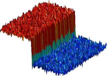
Refer to caption
(a) Original image
Refer to caption
(b) μ𝜇absent\mu\leftarrowadaptive, λ𝜆absent\lambda\leftarrowconstant
Refer to caption
(c) μ𝜇absent\mu\leftarrowconstant, λ𝜆absent\lambda\leftarrowadaptive
Figure 4: (Color Online) The proposed model (stopping parameter ϵ=104italic-ϵsuperscript104\epsilon=10^{-4}) with adaptive μ1subscript𝜇1\mu_{1} (see Eqn. (17)) and constant λ𝜆\lambda (=1absent1=1) provides better edge preservation in the cartoon component and captures small scale oscillations in the texture component against constant μ𝜇\mu (=1absent1=1) and adaptive λ𝜆\lambda (using the definition of μ1subscript𝜇1\mu_{1} from Eqn. (17)).

Here, we consider the data adaptive parameters selection strategies which can provide a balanced approach in obtaining better CTE decomposition results. For the image fidelity parameter μ𝜇\mu in Eqn. (7) we utilize a local histogram measure which was motivated from the image segmentation model of [36]. For a given gray-scale image I:Ω¯[0,L]:𝐼¯Ω0𝐿I:\overline{\Omega}\longrightarrow[0,L], let 𝒩x,rsubscript𝒩𝑥𝑟\mathcal{N}_{{x},r} be the local region centered at x𝑥{x} with radius r𝑟r. We compute the local histogram of the pixel xΩ𝑥Ωx\in\Omega and its corresponding cumulative distribution function

Px(y)=|{z𝒩x,rΩ|I(z)=y}|𝒩x,rΩsubscript𝑃𝑥𝑦conditional-set𝑧subscript𝒩𝑥𝑟Ω𝐼𝑧𝑦subscript𝒩𝑥𝑟Ω\displaystyle P_{x}(y)=\frac{|\{z\in\mathcal{N}_{{x},r}\cap\Omega\,|\,I(z)=y\}|}{\mathcal{N}_{x,r}\cap\Omega} (15)
Fx(y)=|{z𝒩x,rΩ|I(z)y}|𝒩x,rΩsubscript𝐹𝑥𝑦conditional-set𝑧subscript𝒩𝑥𝑟Ω𝐼𝑧𝑦subscript𝒩𝑥𝑟Ω\displaystyle F_{x}(y)=\frac{|\{z\in\mathcal{N}_{{x},r}\cap\Omega\,|\,I(z)\leq y\}|}{\mathcal{N}_{{x},r}\cap\Omega} (16)

for 0yL0𝑦𝐿0\leq y\leq L, respectively. This allows us to define the following measurable function μ:Ω:𝜇Ω\mu:\Omega\rightarrow\mathbb{R}, such that for each xΩ𝑥Ω{x}\in\Omega,

μ(x)=μ1(x)=0LFx(y)𝑑ymaxxΩ0LFx(y)𝑑y,𝜇𝑥subscript𝜇1𝑥superscriptsubscript0𝐿subscript𝐹𝑥𝑦differential-d𝑦subscript𝑥Ωsuperscriptsubscript0𝐿subscript𝐹𝑥𝑦differential-d𝑦\mu(x)=\mu_{1}(x)=\frac{\int_{0}^{L}F_{x}(y)\,dy}{\max\limits_{{x}\in\Omega}\int_{0}^{L}F_{x}(y)\,dy}, (17)

allowing us to get a weight of how much nonhomogeneous intensity is present in a local region 𝒩x,rsubscript𝒩𝑥𝑟\mathcal{N}_{{x},r} of a given pixel x𝑥{x}. This new feature of the image does not depend on the pixel properties instead provides regional properties, see [36] for more details. Thus, we see that the μ𝜇\mu is chosen according to local histogram information and is computed in an image adaptive way using the cartoon unsuperscript𝑢𝑛u^{n} in the iterative scheme (13). We compare our approach with two related adaptive functions:

  1. 1.

    The adaptive formulation of [48] which uses a summation of cartoon components up-to iteration n𝑛n.

    μ2(x)=i=0nGρiun(x)subscript𝜇2𝑥superscriptsubscript𝑖0𝑛subscript𝐺subscript𝜌𝑖superscript𝑢𝑛𝑥\displaystyle\mu_{2}(x)=\sum_{i=0}^{n}G_{\rho_{i}}\star u^{n}(x) (18)

    with ρi=1/i2subscript𝜌𝑖1superscript𝑖2\rho_{i}=1/i^{2} and at n=0𝑛0n=0 the λ2(x)=0.05subscript𝜆2𝑥0.05\lambda_{2}(x)=0.05.

  2. 2.

    Relative reduction rate based parameter proposed in local TV based scheme [30].

    μ3(x)=Gρ|f(x)|Gρ|Lσf(x)|Gρ|f(x)|,subscript𝜇3𝑥subscript𝐺𝜌𝑓𝑥subscript𝐺𝜌subscript𝐿𝜎𝑓𝑥subscript𝐺𝜌𝑓𝑥\displaystyle\mu_{3}(x)=\frac{G_{\rho}\star\left|\nabla f(x)\right|-G_{\rho}\star\left|L_{\sigma}\star\nabla f(x)\right|}{G_{\rho}\star\left|\nabla f(x)\right|}, (19)

    where Lσsubscript𝐿𝜎L_{\sigma} is a low pass filter. Note that this adaptive parameter uses only the initial input image f𝑓f whereas the previous choices use u𝑢u computed at a previous (Eqn. (17)) or every (Eqn. (18)) iteration.

Remark 2.

Figure 4 explains the choice of adaptiveness in our coupled model (7-8) for a synthetic image with different texture patterns. The first case with μ𝜇\mu adaptive, λ𝜆\lambda constant provides persisting cartoon component whereas the second case with μ𝜇\mu constant, λ𝜆\lambda adaptive (same local histogram based measure, Eqn. (17) is used for defining λ(x)𝜆𝑥\lambda(x)) blurs the boundaries in the final result. Thus, in what follows, we use only μ𝜇\mu adaptive parameter to illustrate our decomposition results.

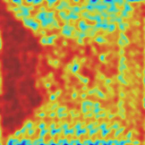
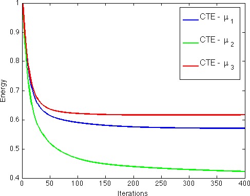
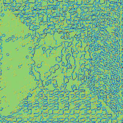
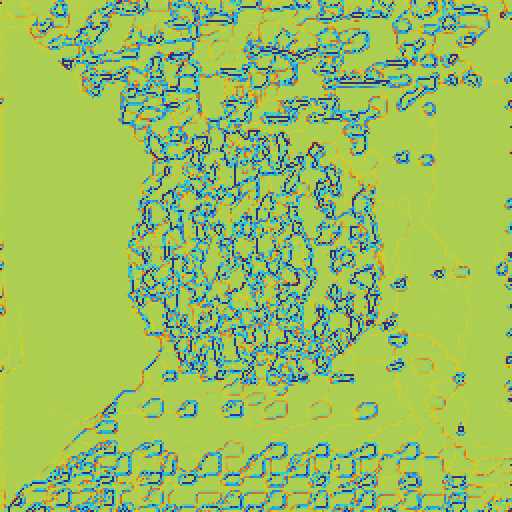
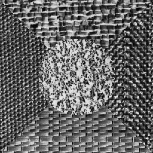
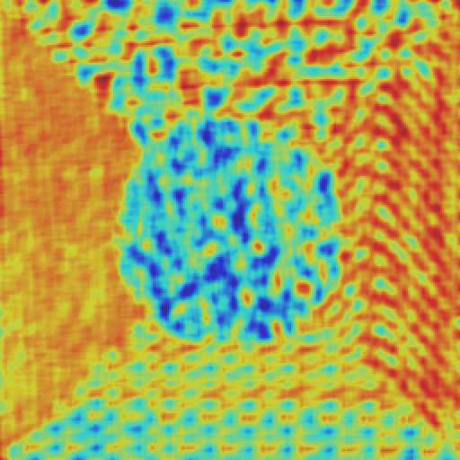
Figure 5 shows a comparison of different adaptive μ𝜇\mu functions for a synthetic texture image. We see that the local histogram based μ1subscript𝜇1\mu_{1} captures the texture components from all the quadrants. Moreover, Figure 5(e) shows that the energy value decreases similarly for different μ𝜇\mu functions as the iteration increases. Figure 6 shows the usage of different μ𝜇\mu function when we apply our model (7-8) for the same synthetic image to obtain cartoon (u𝑢u) + texture (v𝑣v) + pseudo-edges (w) decomposition. Note that the texture image v𝑣v is obtained by linearly transforming its range to [0,255]0255[0,255] for visualization purposes. Differences outside this range are saturated to 00 and 255255255 respectively. A similar transformation is applied to the edges (w𝑤w) component as well. Next, we study the wellposedness of the model (7-8) using weak solutions concept and prove some a priori estimates and solvability of the proposed adaptive coupled model.
Refer to caption
(a) Input (f𝑓f)
Refer to caption
(b) μ1subscript𝜇1\mu_{1}
Refer to caption
(c) μ2subscript𝜇2\mu_{2}
Refer to caption
(d) μ3subscript𝜇3\mu_{3}
Refer to caption
(e) Energy
Figure 5: (Color Online) Comparison of different μ𝜇\mu functions computed using the given input image. (a) Original image. (b) μ1subscript𝜇1\mu_{1} based on local histograms Eqn. (17). (c) μ2subscript𝜇2\mu_{2} based on the work of [48] Eqn. (18). (d) μ3subscript𝜇3\mu_{3} base on the work of [30] Eqn. (19). (e) Energy versus iteration for different adaptive μ𝜇\mu functions based energy minimization scheme (7-8) with stooping parameter ϵ=104italic-ϵsuperscript104\epsilon=10^{-4}.
Refer to caption
Refer to caption
Refer to caption
Refer to caption
Refer to caption
Refer to caption
Refer to caption
Refer to caption
Refer to caption
(a) u𝑢u
Refer to caption
(b) v𝑣v
Refer to caption
(c) w𝑤w
Refer to caption
(d) v+w𝑣𝑤v+w
Figure 6: (Color Online) Different μ𝜇\mu functions based CTE scheme (with λ𝜆\lambda constant) results (stopping parameter ϵ=104italic-ϵsuperscript104\epsilon=10^{-4}). Top: μ1subscript𝜇1\mu_{1} (local histogram) based result. Middle: μ2subscript𝜇2\mu_{2} result. Bottom: μ3subscript𝜇3\mu_{3} result. (a) Cartoon u𝑢u. (b) Texture v𝑣v. (c) Pseudo-edges w𝑤w. (d) v+w𝑣𝑤v+w. Best viewed electronically, zoomed in.

3 Wellposedness

3.1 Preliminaries

In the section, ΩΩ\Omega is considered to be a bounded domain (i.e. an open set in 2superscript2\mathbb{R}^{2}) possessing the cone property. We recall that this means that each point xΩ𝑥Ωx\in\Omega is a vertex of a finite cone Cxsubscript𝐶𝑥C_{x} contained in ΩΩ\Omega, and all these cones Cxsubscript𝐶𝑥C_{x} are congruent [1]. Obviously, rectangular domains have this property. Fix also a time interval [0,T]0𝑇[0,T], T>0𝑇0T>0.

We study wellposedness of the weighted TV regularization,

u(t,x)=𝐮(x):min𝐮:Ω{Ωg(w(t,x))|𝐮(x)|𝑑x+Ωμ(x)|𝐮(x)f(x)|𝑑x},:𝑢𝑡𝑥𝐮𝑥subscript:𝐮ΩsubscriptΩ𝑔𝑤𝑡𝑥𝐮𝑥differential-d𝑥subscriptΩ𝜇𝑥𝐮𝑥𝑓𝑥differential-d𝑥\displaystyle u(t,x)=\mathbf{u}(x):\,\min\limits_{\mathbf{u}:\Omega\to\mathbb{R}}\Bigg{\{}\int_{\Omega}g(w(t,x))|\nabla\mathbf{u}(x)|\,dx+\int_{\Omega}\mu(x)|\mathbf{u}(x)-f(x)|\,dx\Bigg{\}}, (20)

with the diffusion constraint,

w(t,x)t𝑤𝑡𝑥𝑡\displaystyle\frac{\partial w(t,x)}{\partial t} =Δp,λw(t,x)+(1λ(x))(|u(t,x)|w(t,x)),absentsubscriptΔ𝑝𝜆𝑤𝑡𝑥1𝜆𝑥𝑢𝑡𝑥𝑤𝑡𝑥\displaystyle=\Delta_{p,\lambda}w(t,x)+(1-\lambda(x))(|\nabla u(t,x)|-w(t,x)), (21)
w(t,x)𝑤𝑡𝑥\displaystyle w(t,x) =0,xΩ,formulae-sequenceabsent0𝑥Ω\displaystyle=0,\ x\in\partial\Omega, (22)
w(0,x)𝑤0𝑥\displaystyle w(0,x) =F(x),absent𝐹𝑥\displaystyle=F(x), (23)

where p2,𝑝2p\geq 2, and f:Ω,:𝑓Ωf:\Omega\to\mathbb{R}, F:Ω[0,+),:𝐹Ω0F:\Omega\to[0,+\infty), λ:Ω(0,1],:𝜆Ω01\lambda:\Omega\to(0,1], μ:Ω(0,+),:𝜇Ω0\mu:\Omega\to(0,+\infty), g:[0,+)(0,+):𝑔00g:[0,+\infty)\to(0,+\infty) are prescribed functions. The operator Δp,λsubscriptΔ𝑝𝜆\Delta_{p,\lambda} is a weighted p𝑝p-Laplacian:

Δp,λv=λdiv(|v|p2v)(1|v|p2)vλ.subscriptΔ𝑝𝜆𝑣𝜆divsuperscript𝑣𝑝2𝑣1superscript𝑣𝑝2𝑣𝜆\Delta_{p,\lambda}v=\lambda\operatorname{div}(|\nabla v|^{p-2}\nabla v)-(1-|\nabla v|^{p-2})\nabla v\cdot\nabla\lambda. (24)

In particular, for p=2𝑝2p=2 we recover the linear diffusion case. In this section, for the sake of generality, we admit adaptive λ𝜆\lambda and generic g𝑔g. Note that w𝑤w is non-negative by the maximum principle. We consider the Dirichlet boundary condition for w𝑤w, but other boundary conditions can also be handled.

We use the brief notations Lqsubscript𝐿𝑞L_{q} (q1𝑞1q\geq 1), Wqmsuperscriptsubscript𝑊𝑞𝑚W_{q}^{m} (m𝑚m\in\mathbb{R}), W0m,qsubscriptsuperscript𝑊𝑚𝑞0W^{m,q}_{0} (m>0𝑚0m>0) for the Lebesgue and Sobolev spaces on ΩΩ\Omega with values in or2𝑜𝑟superscript2\mathbb{R}\ or\ \mathbb{R}^{2}. Parentheses denote the bilinear form

(u,v)=Ωu(x)v(x)𝑑x.𝑢𝑣subscriptΩ𝑢𝑥𝑣𝑥differential-d𝑥(u,v)=\int\limits_{\Omega}u(x)\cdot v(x)\,dx.

The norm in L2subscript𝐿2L_{2} is u=(u,u)norm𝑢𝑢𝑢\|u\|=\sqrt{(u,u)}.

The symbols S(𝒥;E)𝑆𝒥𝐸S(\mathcal{J};E), C(𝒥;E)𝐶𝒥𝐸C(\mathcal{J};E), L1(𝒥;E)subscript𝐿1𝒥𝐸L_{1}(\mathcal{J};E) denote the spaces of Bochner measurable, continuous, Bochner integrable functions on an interval 𝒥𝒥\mathcal{J}\subset\mathbb{R} with values in a Banach space E𝐸E, respectively.

Let \mathcal{M} be the Banach space of finite Radon measures on ΩΩ\Omega. It is the dual of the space C0(Ω)subscript𝐶0ΩC_{0}(\Omega) (the space of continuous functions on ΩΩ\Omega that vanish at ΩΩ\partial\Omega, see e.g. [23]).

Let BV𝐵𝑉BV be the space of functions of bounded variation on ΩΩ\Omega. For vBV𝑣𝐵𝑉v\in BV, and ϕC(Ω¯)italic-ϕ𝐶¯Ω\phi\in C(\overline{\Omega}), ϕ0italic-ϕ0\phi\geq 0, the weighted total variation of v𝑣v is

TVϕ(v)=supψC0(Ω):|ψ|ϕ(v,divψ).𝑇subscript𝑉italic-ϕ𝑣subscriptsupremum:𝜓superscriptsubscript𝐶0Ω𝜓italic-ϕ𝑣div𝜓TV_{\phi}(v)=\sup\limits_{\psi\in C_{0}^{\infty}(\Omega):\,|\psi|\leq\phi}(v,\operatorname{div}\psi). (25)

In particular, the total variation of u𝑢u is

TV(v)=TV1(v).𝑇𝑉𝑣𝑇subscript𝑉1𝑣TV(v)=TV_{1}(v). (26)

Due to lower semicontinuity of suprema, for every non-negative ϕC(Ω¯)italic-ϕ𝐶¯Ω\phi\in C(\overline{\Omega}) and a weakly-* converging sequence {vm}BVsubscript𝑣𝑚𝐵𝑉\{v_{m}\}\subset BV, we have

TVϕ(v)limm+infTVϕ(vm).𝑇subscript𝑉italic-ϕ𝑣subscript𝑚infimum𝑇subscript𝑉italic-ϕsubscript𝑣𝑚TV_{\phi}(v)\leq\lim_{m\to+\infty}\inf TV_{\phi}(v_{m}). (27)

A more refined argument of the same nature proves

Lemma 1.

For any φS(0,T;C(Ω¯))𝜑𝑆0𝑇𝐶¯Ω\varphi\in S(0,T;C(\overline{\Omega})), φ0𝜑0\varphi\geq 0 for a.a. t(0,T)𝑡0𝑇t\in(0,T), and a weakly-* converging sequence {vm}Lq(0,T;BV)subscript𝑣𝑚subscript𝐿𝑞0𝑇𝐵𝑉\{v_{m}\}\subset L_{q}(0,T;BV), q>1𝑞1q>1, one has

TVφ(t)(v(t))limm+infTVφ(t)(vm(t))𝑇subscript𝑉𝜑𝑡𝑣𝑡subscript𝑚infimum𝑇subscript𝑉𝜑𝑡subscript𝑣𝑚𝑡TV_{\varphi(t)}(v(t))\leq\lim_{m\to+\infty}\inf TV_{\varphi(t)}(v_{m}(t)) (28)

for a.a. t(0,T)𝑡0𝑇t\in(0,T).

For vBV𝑣𝐵𝑉v\in BV, |v|𝑣|\nabla v| will denote the corresponding total variation measure. The operator

|()|:BV:𝐵𝑉|\nabla(\cdot)|:BV\to\mathcal{M} (29)

is bounded. We recall the duality relation

TVϕ(v)=|v|,ϕ×C0(Ω).𝑇subscript𝑉italic-ϕ𝑣subscript𝑣italic-ϕsubscript𝐶0ΩTV_{\phi}(v)=\langle|\nabla v|,\phi\rangle_{\mathcal{M}\times C_{0}(\Omega)}. (30)

The symbol C𝐶C will stand for a generic positive constant that can take different values in different lines. We sometimes write C()𝐶C(\dots) to specify that the constant depends on a certain parameter or value.

We will use the embeddings

BVLq,q2,formulae-sequence𝐵𝑉subscript𝐿𝑞𝑞2BV\subset L_{q},\ q\leq 2, (31)
W21Lq,q<+,formulae-sequencesubscriptsuperscript𝑊12subscript𝐿𝑞𝑞W^{1}_{2}\subset L_{q},\ q<+\infty, (32)
Wp1C(Ω¯),p>2,formulae-sequencesubscriptsuperscript𝑊1𝑝𝐶¯Ω𝑝2W^{1}_{p}\subset C(\overline{\Omega}),\ p>2, (33)

and

Wq1,q<2,formulae-sequencesubscriptsuperscript𝑊1𝑞𝑞2\mathcal{M}\subset W^{-1}_{q},\ q<2, (34)

and the Poincaré inequality

vWp1CvLp,p1,v|Ω=0.formulae-sequencesubscriptnorm𝑣subscriptsuperscript𝑊1𝑝𝐶subscriptnorm𝑣subscript𝐿𝑝formulae-sequence𝑝1evaluated-at𝑣Ω0\|v\|_{W^{1}_{p}}\leq C\|\nabla v\|_{L_{p}},\ p\geq 1,\ v\Big{|}_{\partial\Omega}=0. (35)

Embeddings (31)–(34) are compact (except for (31) with q=2𝑞2q=2).

We assume that λ𝜆\lambda, λ𝜆\nabla\lambda and g𝑔g are Lipschitz functions,

λ0=infxΩλ(x)>0,g0=supy0g(y)<+,formulae-sequencesubscript𝜆0subscriptinfimum𝑥Ω𝜆𝑥0subscript𝑔0subscriptsupremum𝑦0𝑔𝑦\lambda_{0}=\inf_{x\in\Omega}\lambda(x)>0,\quad\quad g_{0}=\sup_{y\geq 0}g(y)<+\infty,

and there exists a constant Cgsubscript𝐶𝑔C_{g} so that

|d(logg(y))dy|Cg1+yfora.a.y0.formulae-sequence𝑑𝑔𝑦𝑑𝑦subscript𝐶𝑔1𝑦foraa𝑦0\Big{|}\frac{d(\log g(y))}{dy}\Big{|}\leq\frac{C_{g}}{1+y}\ \,\mathrm{for\ a.a.}\ y\geq 0. (36)

The last condition means that g𝑔g can have at most polynomial decay at infinity.

We assume that μL(Ω),𝜇subscript𝐿Ω\mu\in L_{\infty}(\Omega), and

0<μ1=essinfxΩμ(x)μ2=esssupxΩμ(x)<+.0subscript𝜇1esssubscriptinfimum𝑥Ω𝜇𝑥subscript𝜇2esssubscriptsupremum𝑥Ω𝜇𝑥0<\mu_{1}=\mathrm{ess}\inf_{x\in\Omega}\mu(x)\leq\mu_{2}=\mathrm{ess}\sup_{x\in\Omega}\mu(x)<+\infty.

Finally, we assume that

FL2,𝐹subscript𝐿2F\in L_{2}, (37)

and at least one of the following three conditions holds:

p>2,fBV,formulae-sequence𝑝2𝑓𝐵𝑉p>2,\,f\in BV, (38)
p=2,q>1:fWq1,:formulae-sequence𝑝2𝑞1𝑓subscriptsuperscript𝑊1𝑞p=2,\,\exists\,q>1:\,f\in W^{1}_{q}, (39)
p=2,fBVL,cg>0:1g(y)cg(1+y),y0.:formulae-sequence𝑝2formulae-sequence𝑓𝐵𝑉subscript𝐿subscript𝑐𝑔0formulae-sequence1𝑔𝑦subscript𝑐𝑔1𝑦𝑦0p=2,\,f\in BV\cap L_{\infty},\,\exists\,c_{g}>0:\,\frac{1}{g(y)}\leq c_{g}(1+y),\ y\geq 0. (40)

3.2 A priori estimates

Before specifying the underlying function spaces and defining the notion of solution, let us derive a formal a priori estimate for problem (20)–(23).

The Euler-Lagrange equation for (20) is

div(g(w)u|u|)+μuf|uf|=0,u/ν|u||Ω=0.formulae-sequencediv𝑔𝑤𝑢𝑢𝜇𝑢𝑓𝑢𝑓0evaluated-at𝑢𝜈𝑢Ω0-\operatorname{div}\left(g(w)\frac{\nabla u}{|\nabla u|}\right)+\mu\frac{u-f}{|u-f|}=0,\ \frac{\partial u/\partial\nu}{|\nabla u|}\Bigg{|}_{\partial\Omega}=0. (41)

For each t[0,T]𝑡0𝑇t\in[0,T], multiplying (41) by w(uf)g(w)𝑤𝑢𝑓𝑔𝑤\frac{w(u-f)}{g(w)}, and integrating over ΩΩ\Omega, we get

(g(w)u|u|,(w(uf)g(w)))+(μwg(w),|uf|)=0.𝑔𝑤𝑢𝑢𝑤𝑢𝑓𝑔𝑤𝜇𝑤𝑔𝑤𝑢𝑓0\left(g(w)\frac{\nabla u}{|\nabla u|},\nabla\left(\frac{w(u-f)}{g(w)}\right)\right)+\left(\frac{\mu w}{g(w)},|u-f|\right)=0. (42)

Thus,

(u|u|,w(uf))(u|u|,g(w)wg(w)w(uf))+(w,|u|)(wu|u|,f)+(μwg(w),|uf|)=0.𝑢𝑢𝑤𝑢𝑓𝑢𝑢superscript𝑔𝑤𝑤𝑔𝑤𝑤𝑢𝑓𝑤𝑢𝑤𝑢𝑢𝑓𝜇𝑤𝑔𝑤𝑢𝑓0\left(\frac{\nabla u}{|\nabla u|},\nabla w(u-f)\right)-\left(\frac{\nabla u}{|\nabla u|},\frac{g^{\prime}(w)w}{g(w)}\nabla w(u-f)\right)\\ +\left(w,|\nabla u|\right)-\left(w\frac{\nabla u}{|\nabla u|},\nabla f\right)+\left(\frac{\mu w}{g(w)},|u-f|\right)=0. (43)

Multiplying (41) by ufg(w)𝑢𝑓𝑔𝑤\frac{u-f}{g(w)}, and integrating over ΩΩ\Omega, we find

(u|u|,g(w)g(w)w(uf))+(1,|u|)(u|u|,f)+(μg(w),|uf|)=0.𝑢𝑢superscript𝑔𝑤𝑔𝑤𝑤𝑢𝑓1𝑢𝑢𝑢𝑓𝜇𝑔𝑤𝑢𝑓0\displaystyle-\left(\frac{\nabla u}{|\nabla u|},\frac{g^{\prime}(w)}{g(w)}\nabla w(u-f)\right)+\left(1,|\nabla u|\right)-\left(\frac{\nabla u}{|\nabla u|},\nabla f\right)+\left(\frac{\mu}{g(w)},|u-f|\right)=0. (44)

Since the last term is non-negative, we conclude that

TV(u)TV(f)+Cgwuf.𝑇𝑉𝑢𝑇𝑉𝑓subscript𝐶𝑔norm𝑤norm𝑢𝑓TV(u)\leq TV(f)+C_{g}\|\nabla w\|\|u-f\|. (45)

Multiplying (41) by uf𝑢𝑓u-f, and integrating over ΩΩ\Omega, we derive

(g(w),|u|)+μ(uf)L1g0TV(f)𝑔𝑤𝑢subscriptnorm𝜇𝑢𝑓subscript𝐿1subscript𝑔0𝑇𝑉𝑓(g(w),|\nabla u|)+\|\mu(u-f)\|_{L_{1}}\leq g_{0}\,TV(f) (46)

Multiplying (41) by u|u|𝑢𝑢u|u|, and integrating over ΩΩ\Omega, we deduce

2(g(w)|u|,|u|)+(uf|uf|,μu|u|).2𝑔𝑤𝑢𝑢𝑢𝑓𝑢𝑓𝜇𝑢𝑢2(g(w)|u|,|\nabla u|)+\left(\frac{u-f}{|u-f|},\mu u|u|\right). (47)

It is not difficult to obtain the following scalar inequality

|ab|32(ab)a|a|+2b2|ab|,a,b,formulae-sequencesuperscript𝑎𝑏32𝑎𝑏𝑎𝑎2superscript𝑏2𝑎𝑏𝑎𝑏|a-b|^{3}\leq 2(a-b)a|a|+2b^{2}|a-b|,\ a,b\in\mathbb{R}, (48)

which enables to conclude from (47) that

μ(uf)2+4(g(w)|u|,|u|)2μf2.superscriptnorm𝜇𝑢𝑓24𝑔𝑤𝑢𝑢2superscriptnorm𝜇𝑓2\|\sqrt{\mu}(u-f)\|^{2}+4(g(w)|u|,|\nabla u|)\leq 2\|\sqrt{\mu}f\|^{2}. (49)

Hence, due to (31),

ufC(f)C(fBV).norm𝑢𝑓𝐶norm𝑓𝐶subscriptnorm𝑓𝐵𝑉\|u-f\|\leq C(\|f\|)\leq C(\|f\|_{BV}). (50)

By (45) and (50),

TV(u)C(1+w).𝑇𝑉𝑢𝐶1norm𝑤TV(u)\leq C(1+\|\nabla w\|). (51)

Multiplying (21) by w𝑤w, and integrating over ΩΩ\Omega, we get

12dw2dt+(λ,|w|p)+((1λ)w,w)=((1λ)w,|u|)(wλ,w).12𝑑superscriptnorm𝑤2𝑑𝑡𝜆superscript𝑤𝑝1𝜆𝑤𝑤1𝜆𝑤𝑢𝑤𝜆𝑤\displaystyle\frac{1}{2}\frac{d\|w\|^{2}}{dt}+(\lambda,|\nabla w|^{p})+((1-\lambda)w,w)=((1-\lambda)w,|\nabla u|)-(w\nabla\lambda,\nabla w). (52)

Using Hölder’s inequality and (36), we deduce from (43) that

(w,|u|)(1+Cg)wLpufLp/p1+(w,|f|).𝑤𝑢1subscript𝐶𝑔subscriptnorm𝑤subscript𝐿𝑝subscriptnorm𝑢𝑓subscript𝐿𝑝𝑝1𝑤𝑓\left(w,|\nabla u|\right)\leq(1+C_{g})\|\nabla w\|_{L_{p}}\|u-f\|_{L_{p/p-1}}+(w,|\nabla f|). (53)

From (52), (53) and Young’s inequality we infer

12dw2dt+λ02wLppC(g,λ0,p)ufLp/p1p/p1+C(λ,p)wLp/p1p/p1+(w,|f|).12𝑑superscriptnorm𝑤2𝑑𝑡subscript𝜆02subscriptsuperscriptnorm𝑤𝑝subscript𝐿𝑝𝐶𝑔subscript𝜆0𝑝superscriptsubscriptnorm𝑢𝑓subscript𝐿𝑝𝑝1𝑝𝑝1𝐶𝜆𝑝superscriptsubscriptnorm𝑤subscript𝐿𝑝𝑝1𝑝𝑝1𝑤𝑓\displaystyle\frac{1}{2}\frac{d\|w\|^{2}}{dt}+\frac{\lambda_{0}}{2}\|\nabla w\|^{p}_{L_{p}}\leq C(g,\lambda_{0},p)\|u-f\|_{L_{p/p-1}}^{p/p-1}+C(\lambda,p)\|w\|_{L_{p/p-1}}^{p/p-1}+(w,|\nabla f|). (54)

Provided (38) or (39), estimate (50), and embeddings (33) or (32), resp., imply

dw2dt+λ0wLppC(1+wp/p1+wWp1).𝑑superscriptnorm𝑤2𝑑𝑡subscript𝜆0subscriptsuperscriptnorm𝑤𝑝subscript𝐿𝑝𝐶1superscriptnorm𝑤𝑝𝑝1subscriptnorm𝑤superscriptsubscript𝑊𝑝1\frac{d\|w\|^{2}}{dt}+\lambda_{0}\|\nabla w\|^{p}_{L_{p}}\leq C(1+\|w\|^{p/p-1}+\|w\|_{W_{p}^{1}}). (55)

By (35),(37) and usual arguments, (55) yields

wL(0,T;L2)+wLp(0,T;W01,p)C.subscriptnorm𝑤subscript𝐿0𝑇subscript𝐿2subscriptnorm𝑤subscript𝐿𝑝0𝑇subscriptsuperscript𝑊1𝑝0𝐶\|w\|_{L_{\infty}(0,T;L_{2})}+\|w\|_{L_{p}(0,T;W^{1,p}_{0})}\leq C. (56)

In case (40), we multiply (41) by wug(w)𝑤𝑢𝑔𝑤\frac{wu}{g(w)}, and integrate over ΩΩ\Omega, arriving at

(u|u|,uw)(u|u|,ug(w)wg(w)w)+(w,|u|)+(μwg(w),|uf|)+(uf|uf|,μwfg(w))=0.𝑢𝑢𝑢𝑤𝑢𝑢𝑢superscript𝑔𝑤𝑤𝑔𝑤𝑤𝑤𝑢𝜇𝑤𝑔𝑤𝑢𝑓𝑢𝑓𝑢𝑓𝜇𝑤𝑓𝑔𝑤0\left(\frac{\nabla u}{|\nabla u|},u\nabla w\right)-\left(\frac{\nabla u}{|\nabla u|},u\frac{g^{\prime}(w)w}{g(w)}\nabla w\right)+\left(w,|\nabla u|\right)\\ +\left(\frac{\mu w}{g(w)},|u-f|\right)+\left(\frac{u-f}{|u-f|},\frac{\mu wf}{g(w)}\right)=0. (57)

Then, since the penultimate term is non-negative,

(w,|u|)(1+Cg)wu+μ2cg(|f|w,1+w)C(1+w+w2).𝑤𝑢1subscript𝐶𝑔delimited-∥∥𝑤delimited-∥∥𝑢subscript𝜇2subscript𝑐𝑔𝑓𝑤1𝑤𝐶1delimited-∥∥𝑤superscriptdelimited-∥∥𝑤2\left(w,|\nabla u|\right)\leq(1+C_{g})\|\nabla w\|\,\|u\|+\mu_{2}c_{g}(|f|w,1+w)\\ \leq C(1+\|\nabla w\|+\|w\|^{2}). (58)

Now, (52) and (58) yield

dw2dt+λ0wLppC(1+w2),𝑑superscriptnorm𝑤2𝑑𝑡subscript𝜆0subscriptsuperscriptnorm𝑤𝑝subscript𝐿𝑝𝐶1superscriptnorm𝑤2\frac{d\|w\|^{2}}{dt}+\lambda_{0}\|\nabla w\|^{p}_{L_{p}}\leq C(1+\|w\|^{2}), (59)

which implies (56). In all the three cases, (46), (51) and (56) imply

uL(0,T;L1)+uLp(0,T;BV)C.subscriptnorm𝑢subscript𝐿0𝑇subscript𝐿1subscriptnorm𝑢subscript𝐿𝑝0𝑇𝐵𝑉𝐶\|u\|_{L_{\infty}(0,T;L_{1})}+\|u\|_{L_{p}(0,T;BV)}\leq C. (60)

The operator

Λ:BV,:Λ𝐵𝑉\Lambda:BV\to\mathcal{M},
Λ(v)=(1λ)|v|,Λ𝑣1𝜆𝑣\Lambda(v)=(1-\lambda)|\nabla v|,
Λ(v),ϕ×C0(Ω)=|v|,(1λ)ϕ×C0(Ω),subscriptΛ𝑣italic-ϕsubscript𝐶0Ωsubscript𝑣1𝜆italic-ϕsubscript𝐶0Ω\langle\Lambda(v),\phi\rangle_{\mathcal{M}\times C_{0}(\Omega)}=\langle|\nabla v|,(1-\lambda)\phi\rangle_{\mathcal{M}\times C_{0}(\Omega)},

is bounded, so

(1λ)|u|Lp(0,T;)C.subscriptnorm1𝜆𝑢subscript𝐿𝑝0𝑇𝐶\|(1-\lambda)|\nabla u|\|_{L_{p}(0,T;\mathcal{M})}\leq C. (61)

The weighted p𝑝p-Laplacian operator

Δp,λ:W01,pWp/p11:subscriptΔ𝑝𝜆subscriptsuperscript𝑊1𝑝0subscriptsuperscript𝑊1𝑝𝑝1\Delta_{p,\lambda}:W^{1,p}_{0}\to W^{-1}_{p/p-1}

is also bounded. Hence, (21),(34),(56) and (61) yield an estimate for the time derivative of w𝑤w:

wLp(0,T;Wq1)C,q<2,qq1p.formulae-sequencesubscriptnormsuperscript𝑤subscript𝐿𝑝0𝑇subscriptsuperscript𝑊1𝑞𝐶formulae-sequence𝑞2𝑞𝑞1𝑝\|w^{\prime}\|_{L_{p}(0,T;W^{-1}_{q})}\leq C,\ q<2,\frac{q}{q-1}\geq p. (62)

3.3 Solvability

Definition 1.

Assume (37) and (38). A pair of functions (u,w)𝑢𝑤(u,w) from the class

uL(0,T;L1)Lp(0,T;BV),𝑢subscript𝐿0𝑇subscript𝐿1subscript𝐿𝑝0𝑇𝐵𝑉u\in L_{\infty}(0,T;L_{1})\cap L_{p}(0,T;BV),
wL(0,T;L2)Lp(0,T;W01,p)Wp1(0,T;Wp/p11),𝑤subscript𝐿0𝑇subscript𝐿2subscript𝐿𝑝0𝑇subscriptsuperscript𝑊1𝑝0superscriptsubscript𝑊𝑝10𝑇subscriptsuperscript𝑊1𝑝𝑝1w\in L_{\infty}(0,T;L_{2})\cap L_{p}(0,T;W^{1,p}_{0})\cap W_{p}^{1}(0,T;W^{-1}_{p/p-1}),

is called a weak solution to problem (20)–(23) if

TVg(w(t))(u(t))+μ(u(t)f)L1TVg(w(t))(𝐮(t))+μ(𝐮(t)f)L1,𝑇subscript𝑉𝑔𝑤𝑡𝑢𝑡subscriptnorm𝜇𝑢𝑡𝑓subscript𝐿1𝑇subscript𝑉𝑔𝑤𝑡𝐮𝑡subscriptnorm𝜇𝐮𝑡𝑓subscript𝐿1\displaystyle TV_{g(w(t))}(u(t))+\|\mu(u(t)-f)\|_{L_{1}}\leq TV_{g(w(t))}(\mathbf{u}(t))+\|\mu(\mathbf{u}(t)-f)\|_{L_{1}}, (63)

for any 𝐮S(0,T;BV)𝐮𝑆0𝑇𝐵𝑉\mathbf{u}\in S(0,T;BV) and a.a. t(0,T)𝑡0𝑇t\in(0,T),

wΔp,λ+(1λ)w=(1λ)|u|superscript𝑤subscriptΔ𝑝𝜆1𝜆𝑤1𝜆𝑢w^{\prime}-\Delta_{p,\lambda}+(1-\lambda)w=(1-\lambda)|\nabla u| (64)

in the space Wp/p11subscriptsuperscript𝑊1𝑝𝑝1W^{-1}_{p/p-1} for a.a. t(0,T)𝑡0𝑇t\in(0,T), and

w(0)=F𝑤0𝐹w(0)=F (65)

in Wp/p11subscriptsuperscript𝑊1𝑝𝑝1W^{-1}_{p/p-1}.

Remark 3.

This definition is correct since all members of (64) belong to Wp/p11subscriptsuperscript𝑊1𝑝𝑝1W^{-1}_{p/p-1} for a.a. t(0,T)𝑡0𝑇t\in(0,T) (cf. the end of Subsection 3.2), and wWp1(0,T;Wp/p11)C([0,T];Wp/p11)𝑤superscriptsubscript𝑊𝑝10𝑇subscriptsuperscript𝑊1𝑝𝑝1𝐶0𝑇subscriptsuperscript𝑊1𝑝𝑝1w\in W_{p}^{1}(0,T;W^{-1}_{p/p-1})\subset C([0,T];W^{-1}_{p/p-1}).

Theorem 1.

Assume (37) and (38). Then there exists a weak solution to (20)–(23).

Proof.

We can prove the existence of weak solutions via approximation of (20)–(23) by a more regular problem, and consequent passage to the limit (cf. [48, 60]). Let (um,wm)subscript𝑢𝑚subscript𝑤𝑚(u_{m},w_{m}) be a sequence of “approximate” solutions (possibly with “approximate” data fmsubscript𝑓𝑚f_{m} and Fmsubscript𝐹𝑚F_{m}). It essentially suffices to show that (63)–(65) is the limiting case of (20)–(23), i.e., that it is possible to pass to the limit in all the members.

Due to estimates (56), (60), (62), without loss of generality we may suppose that

umuweaklyinL(0,T;),u_{m}\to u\ \mathrm{weakly-*\ in}\ L_{\infty}(0,T;\mathcal{M}), (66)
umuweaklyinLp(0,T;BV),u_{m}\to u\ \mathrm{weakly-*\ in}\ L_{p}(0,T;BV), (67)
wmwweaklyinL(0,T;L2),w_{m}\to w\ \mathrm{weakly-*\ in}\ L_{\infty}(0,T;L_{2}), (68)
wmwweaklyinLp(0,T;W01,p),subscript𝑤𝑚𝑤weaklyinsubscript𝐿𝑝0𝑇subscriptsuperscript𝑊1𝑝0w_{m}\to w\ \mathrm{weakly\ in}\ L_{p}(0,T;W^{1,p}_{0}), (69)
wmwweaklyinLp(0,T;Wp/p11).subscriptsuperscript𝑤𝑚superscript𝑤weaklyinsubscript𝐿𝑝0𝑇subscriptsuperscript𝑊1𝑝𝑝1w^{\prime}_{m}\to w^{\prime}\ \mathrm{weakly\ in}\ L_{p}(0,T;W^{-1}_{p/p-1}). (70)

Note that

uL(0,T;L1)L(0,T;)Lp(0,T;BV).𝑢subscript𝐿0𝑇subscript𝐿1subscript𝐿0𝑇subscript𝐿𝑝0𝑇𝐵𝑉u\in L_{\infty}(0,T;L_{1})\subset L_{\infty}(0,T;\mathcal{M})\cap L_{p}(0,T;BV). (71)

By (33), (34) and the Aubin-Lions-Simon theorem [60],

wmwstronglyinLp(0,T;C(Ω¯)),subscript𝑤𝑚𝑤stronglyinsubscript𝐿𝑝0𝑇𝐶¯Ωw_{m}\to w\ \mathrm{strongly\ in}\ L_{p}(0,T;C(\overline{\Omega})), (72)
wmwstronglyinC([0,T];Wp/p11),subscript𝑤𝑚𝑤stronglyin𝐶0𝑇subscriptsuperscript𝑊1𝑝𝑝1w_{m}\to w\ \mathrm{strongly\ in}\ C([0,T];W^{-1}_{p/p-1}), (73)

so

wm(0)w(0)inWp/p11,subscript𝑤𝑚0𝑤0insubscriptsuperscript𝑊1𝑝𝑝1w_{m}(0)\to w(0)\ \mathrm{in}\ W^{-1}_{p/p-1}, (74)

and we can pass to the limit in (65).

Using the representation

vL1=supφL,φL1(φ,v),subscriptnorm𝑣subscript𝐿1subscriptsupremumformulae-sequence𝜑subscript𝐿subscriptnorm𝜑subscript𝐿1𝜑𝑣\|v\|_{L_{1}}=\sup\limits_{\varphi\in L_{\infty},\,\|\varphi\|_{L_{\infty}}\leq 1}(\varphi,v), (75)

and lower semicontinuity of suprema, we can check that

μ(u(t)f)L1subscriptnorm𝜇𝑢𝑡𝑓subscript𝐿1\displaystyle\|\mu(u(t)-f)\|_{L_{1}} limm+infμ(um(t)f)L1absentsubscript𝑚infimumsubscriptnorm𝜇subscript𝑢𝑚𝑡𝑓subscript𝐿1\displaystyle\leq\lim_{m\to+\infty}\inf\|\mu(u_{m}(t)-f)\|_{L_{1}}
=limm+infμ(um(t)fm)L1absentsubscript𝑚infimumsubscriptnorm𝜇subscript𝑢𝑚𝑡subscript𝑓𝑚subscript𝐿1\displaystyle=\lim_{m\to+\infty}\inf\|\mu(u_{m}(t)-f_{m})\|_{L_{1}} (76)

for a.a. t(0,T)𝑡0𝑇t\in(0,T). By Lemma 1,

TVg(w(t))(u(t))limm+infTVg(w(t))(um(t)).𝑇subscript𝑉𝑔𝑤𝑡𝑢𝑡subscript𝑚infimum𝑇subscript𝑉𝑔𝑤𝑡subscript𝑢𝑚𝑡TV_{g(w(t))}(u(t))\leq\lim_{m\to+\infty}\inf TV_{g(w(t))}(u_{m}(t)). (77)

But

|TVg(wm(t))(um(t))TVg(w(t))(um(t))|g(wm(t))g(w(t))LTV(um(t))C(g)wm(t)w(t)LTV(um(t)),𝑇subscript𝑉𝑔subscript𝑤𝑚𝑡subscript𝑢𝑚𝑡𝑇subscript𝑉𝑔𝑤𝑡subscript𝑢𝑚𝑡subscriptdelimited-∥∥𝑔subscript𝑤𝑚𝑡𝑔𝑤𝑡subscript𝐿𝑇𝑉subscript𝑢𝑚𝑡𝐶𝑔subscriptdelimited-∥∥subscript𝑤𝑚𝑡𝑤𝑡subscript𝐿𝑇𝑉subscript𝑢𝑚𝑡|TV_{g(w_{m}(t))}(u_{m}(t))-TV_{g(w(t))}(u_{m}(t))|\\ \leq\|g(w_{m}(t))-g(w(t))\|_{L_{\infty}}TV(u_{m}(t))\leq C(g)\|w_{m}(t)-w(t)\|_{L_{\infty}}TV(u_{m}(t)), (78)

so

TVg(wm)(um)TVg(w)(um)Lp/2(0,T)CwmwLp(0,T;L)umLp(0,T;BV)0.subscriptnorm𝑇subscript𝑉𝑔subscript𝑤𝑚subscript𝑢𝑚𝑇subscript𝑉𝑔𝑤subscript𝑢𝑚subscript𝐿𝑝20𝑇𝐶subscriptnormsubscript𝑤𝑚𝑤subscript𝐿𝑝0𝑇subscript𝐿subscriptnormsubscript𝑢𝑚subscript𝐿𝑝0𝑇𝐵𝑉0\displaystyle\|TV_{g(w_{m})}(u_{m})-TV_{g(w)}(u_{m})\|_{L_{p/2}(0,T)}\leq C\|w_{m}-w\|_{L_{p}(0,T;L_{\infty})}\|u_{m}\|_{L_{p}(0,T;BV)}\to 0. (79)

Therefore, without loss of generality,

TVg(wm(t))(um(t))TVg(w(t))(um(t))0𝑇subscript𝑉𝑔subscript𝑤𝑚𝑡subscript𝑢𝑚𝑡𝑇subscript𝑉𝑔𝑤𝑡subscript𝑢𝑚𝑡0TV_{g(w_{m}(t))}(u_{m}(t))-TV_{g(w(t))}(u_{m}(t))\to 0 (80)

for a.a. t(0,T)𝑡0𝑇t\in(0,T). Due to (76), (77), (80), we can pass to the limit in (63).

On the other hand, (63) with u=um𝑢subscript𝑢𝑚u=u_{m}, f=fm𝑓subscript𝑓𝑚f=f_{m}, w=wm𝑤subscript𝑤𝑚w=w_{m}, 𝐮=u𝐮𝑢\mathbf{u}=u gives

TVg(wm(t))(um(t))+μ(um(t)fm)L1TVg(wm(t))(u(t))+μ(u(t)fm)L1.𝑇subscript𝑉𝑔subscript𝑤𝑚𝑡subscript𝑢𝑚𝑡subscriptnorm𝜇subscript𝑢𝑚𝑡subscript𝑓𝑚subscript𝐿1𝑇subscript𝑉𝑔subscript𝑤𝑚𝑡𝑢𝑡subscriptnorm𝜇𝑢𝑡subscript𝑓𝑚subscript𝐿1\displaystyle TV_{g(w_{m}(t))}(u_{m}(t))+\|\mu(u_{m}(t)-f_{m})\|_{L_{1}}\leq TV_{g(w_{m}(t))}(u(t))+\|\mu(u(t)-f_{m})\|_{L_{1}}. (81)

Similarly to (78)–(80), we can check that

TVg(wm(t))(u(t))TVg(w(t))(u(t))0.𝑇subscript𝑉𝑔subscript𝑤𝑚𝑡𝑢𝑡𝑇subscript𝑉𝑔𝑤𝑡𝑢𝑡0TV_{g(w_{m}(t))}(u(t))-TV_{g(w(t))}(u(t))\to 0. (82)

From (76), (77), (80)–(82) we conclude that

TVg(w(t))(um(t))TVg(w(t))(u(t))𝑇subscript𝑉𝑔𝑤𝑡subscript𝑢𝑚𝑡𝑇subscript𝑉𝑔𝑤𝑡𝑢𝑡TV_{g(w(t))}(u_{m}(t))\to TV_{g(w(t))}(u(t)) (83)

for a.a. t(0,T)𝑡0𝑇t\in(0,T).

Fix any non-negative function ϕC0(Ω)italic-ϕsubscript𝐶0Ω\phi\in C_{0}(\Omega). Let

κ(t)=ϕg(w(t))L𝜅𝑡subscriptnormitalic-ϕ𝑔𝑤𝑡𝐿\kappa(t)=\left\|\frac{\phi}{g(w(t))}\right\|_{L\infty} (84)

and

φ(t)=κ(t)g(w(t))ϕ.𝜑𝑡𝜅𝑡𝑔𝑤𝑡italic-ϕ\varphi(t)=\kappa(t)g(w(t))-\phi. (85)

For a.a. t(0,T)𝑡0𝑇t\in(0,T), φ(t)𝜑𝑡\varphi(t) is a non-negative continuous function on Ω¯¯Ω\overline{\Omega}. By Lemma 1 and (83), we infer that

TVϕ(u(t))=κ(t)TVg(w(t))(u(t))TVφ(t)(u(t))limm+sup(κ(t)TVg(w(t))(um(t))TVφ(t)(um(t)))=limm+supTVϕ(um(t)).𝑇subscript𝑉italic-ϕ𝑢𝑡𝜅𝑡𝑇subscript𝑉𝑔𝑤𝑡𝑢𝑡𝑇subscript𝑉𝜑𝑡𝑢𝑡subscript𝑚supremum𝜅𝑡𝑇subscript𝑉𝑔𝑤𝑡subscript𝑢𝑚𝑡𝑇subscript𝑉𝜑𝑡subscript𝑢𝑚𝑡subscript𝑚supremum𝑇subscript𝑉italic-ϕsubscript𝑢𝑚𝑡TV_{\phi}(u(t))=\kappa(t)TV_{g(w(t))}(u(t))-TV_{\varphi(t)}(u(t))\geq\lim_{m\to+\infty}\sup(\kappa(t)TV_{g(w(t))}(u_{m}(t))-TV_{\varphi(t)}(u_{m}(t)))\\ =\lim_{m\to+\infty}\sup TV_{\phi}(u_{m}(t)). (86)

But, due to (28),

TVϕ(u(t))limm+infTVϕ(um(t)).𝑇subscript𝑉italic-ϕ𝑢𝑡subscript𝑚infimum𝑇subscript𝑉italic-ϕsubscript𝑢𝑚𝑡TV_{\phi}(u(t))\leq\lim_{m\to+\infty}\inf TV_{\phi}(u_{m}(t)). (87)

Thus,

TVϕ(u(t))=limm+TVϕ(um(t)),𝑇subscript𝑉italic-ϕ𝑢𝑡subscript𝑚𝑇subscript𝑉italic-ϕsubscript𝑢𝑚𝑡TV_{\phi}(u(t))=\lim_{m\to+\infty}TV_{\phi}(u_{m}(t)), (88)

for every non-negative ϕC0(Ω)italic-ϕsubscript𝐶0Ω\phi\in C_{0}(\Omega), which yields

|um(t)||u(t)|subscript𝑢𝑚𝑡𝑢𝑡|\nabla u_{m}(t)|\to|\nabla u(t)| (89)

weakly-* in \mathcal{M} for a.a. t(0,T)𝑡0𝑇t\in(0,T). Then (34) implies

(1λ)|um(t)|(1λ)|u(t)|1𝜆subscript𝑢𝑚𝑡1𝜆𝑢𝑡(1-\lambda)|\nabla u_{m}(t)|\to(1-\lambda)|\nabla u(t)| (90)

strongly in Wp/p11subscriptsuperscript𝑊1𝑝𝑝1W^{-1}_{p/p-1} for a.a. t(0,T)𝑡0𝑇t\in(0,T). Due to (67) and (34),

(1λ)|um|Lp(0,T;Wp/p11)C.subscriptnorm1𝜆subscript𝑢𝑚subscript𝐿𝑝0𝑇subscriptsuperscript𝑊1𝑝𝑝1𝐶\|(1-\lambda)|\nabla u_{m}|\|_{L_{p}(0,T;W^{-1}_{p/p-1})}\leq C. (91)

By (90), (91) and [35, Proposition 2.8, Remark 2.10],

(1λ)|um|(1λ)|u|stronglyinLq(0,T;Wp/p11),q<p.formulae-sequence1𝜆subscript𝑢𝑚1𝜆𝑢stronglyinsubscript𝐿𝑞0𝑇subscriptsuperscript𝑊1𝑝𝑝1for-all𝑞𝑝\displaystyle(1-\lambda)|\nabla u_{m}|\to(1-\lambda)|\nabla u|\mathrm{strongly\ in}\ L_{q}(0,T;W^{-1}_{p/p-1}),\ \forall q<p. (92)

Rewrite (64) as

w+Aw=K(u,w),superscript𝑤𝐴𝑤𝐾𝑢𝑤w^{\prime}+Aw=K(u,w), (93)

where

A(w)=div(λ|w|p2w)+(1λ)w,K(u,w)=wλ+(1λ)|u|.formulae-sequence𝐴𝑤div𝜆superscript𝑤𝑝2𝑤1𝜆𝑤𝐾𝑢𝑤𝑤𝜆1𝜆𝑢\displaystyle A(w)=-\operatorname{div}(\lambda|\nabla w|^{p-2}\nabla w)+(1-\lambda)w,\ K(u,w)=-\nabla w\cdot\nabla\lambda+(1-\lambda)|\nabla u|. (94)

It is easy to see that the operator A:W01,pWp/p11:𝐴subscriptsuperscript𝑊1𝑝0subscriptsuperscript𝑊1𝑝𝑝1A:W^{1,p}_{0}\to W^{-1}_{p/p-1} is monotone, coercive and hemi-continuous (cf. [33]). By (72) and (92),

K(um,wm)K(u,w)stronglyinLp/p1(0,T;Wp/p11).𝐾subscript𝑢𝑚subscript𝑤𝑚𝐾𝑢𝑤stronglyinsubscript𝐿𝑝𝑝10𝑇subscriptsuperscript𝑊1𝑝𝑝1K(u_{m},w_{m})\to K(u,w)\ \mathrm{strongly\ in}\ L_{p/p-1}(0,T;W^{-1}_{p/p-1}).

Hence, we can successfully pass to the limit in (93) via Minty-Browder monotonicity technique (cf. [33]). ∎

Definition 2.

Assume (37) and (39) or (40). A pair of functions (u,w)𝑢𝑤(u,w) from the class

uL(0,T;L1)L2(0,T;BV),𝑢subscript𝐿0𝑇subscript𝐿1subscript𝐿20𝑇𝐵𝑉u\in L_{\infty}(0,T;L_{1})\cap L_{2}(0,T;BV), (95)
wL(0,T;L2)L2(0,T;W01,2)W21(0,T;Wq1),q<2,formulae-sequence𝑤subscript𝐿0𝑇subscript𝐿2subscript𝐿20𝑇subscriptsuperscript𝑊120superscriptsubscript𝑊210𝑇subscriptsuperscript𝑊1𝑞for-all𝑞2w\in L_{\infty}(0,T;L_{2})\cap L_{2}(0,T;W^{1,2}_{0})\cap W_{2}^{1}(0,T;W^{-1}_{q}),\ \forall q<2, (96)

is called a pseudosolution to problem (20)–(23) if there is a sequence (um,wm,pm)subscript𝑢𝑚subscript𝑤𝑚subscript𝑝𝑚(u_{m},w_{m},p_{m}) such that each pair (um,wm)subscript𝑢𝑚subscript𝑤𝑚(u_{m},w_{m}) is a weak solution to (20)–(23) with p=pm𝑝subscript𝑝𝑚p=p_{m},

umuweaklyinL(0,T;),u_{m}\to u\ \mathrm{weakly-*\ in}\ L_{\infty}(0,T;\mathcal{M}),
umuweaklyinL2(0,T;BV),u_{m}\to u\ \mathrm{weakly-*\ in}\ L_{2}(0,T;BV),
wmwweaklyinL(0,T;L2),w_{m}\to w\ \mathrm{weakly-*\ in}\ L_{\infty}(0,T;L_{2}),
wmwweaklyinL2(0,T;W01,2),subscript𝑤𝑚𝑤weaklyinsubscript𝐿20𝑇subscriptsuperscript𝑊120w_{m}\to w\ \mathrm{weakly\ in}\ L_{2}(0,T;W^{1,2}_{0}),
wmwstronglyinL2(0,T;Lq),q<+,formulae-sequencesubscript𝑤𝑚𝑤stronglyinsubscript𝐿20𝑇subscript𝐿𝑞for-all𝑞w_{m}\to w\ \mathrm{strongly\ in}\ L_{2}(0,T;L_{q}),\ \forall q<+\infty,
wmwstronglyinC([0,T];Wq1),q<2,formulae-sequencesubscript𝑤𝑚𝑤stronglyin𝐶0𝑇subscriptsuperscript𝑊1𝑞for-all𝑞2w_{m}\to w\ \mathrm{strongly\ in}\ C([0,T];W^{-1}_{q}),\ \forall q<2,
wmwweaklyinL2(0,T;Wq1),q<2,formulae-sequencesubscriptsuperscript𝑤𝑚superscript𝑤weaklyinsubscript𝐿20𝑇subscriptsuperscript𝑊1𝑞for-all𝑞2w^{\prime}_{m}\to w^{\prime}\ \mathrm{weakly\ in}\ L_{2}(0,T;W^{-1}_{q}),\ \forall q<2,
pm2.subscript𝑝𝑚2p_{m}\to 2.
Theorem 2.

Assume (37) and (39) or (40). Then there exists a pseudosolution to (20)–(23).

Proof.

The proof is based on estimates (56), (60), (62) and the proof of Theorem 1. ∎

4 Experimental Results

4.1 Implementation details

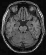
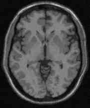
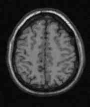
The proposed scheme is implemented using the dual minimization [14] for the weighted TV (Eqn. (7)) and explicit Euler finite difference scheme for the non-homogenous linear diffusion (Eqn. (8)). The edge indicator function g(w)=1/(1+w2)𝑔𝑤11superscript𝑤2g(w)=1/(1+w^{2}) is used for all the results reported here. We obtained similar results for other g𝑔g functions. The adaptive μ1subscript𝜇1\mu_{1} based results are reported here unless otherwise stated explicitly and μ2subscript𝜇2\mu_{2} provided similar results whereas μ3subscript𝜇3\mu_{3} provided slightly blurred cartoon components, see Section 2.3 for details. The parameters δx=1𝛿𝑥1\delta x=1, δt=1/8𝛿𝑡18\delta t=1/8 and θ=102𝜃superscript102\theta=10^{-2} are fixed, and the best results according to the max𝑚𝑎𝑥max(|un+1un|superscript𝑢𝑛1superscript𝑢𝑛\left|u^{n+1}-u^{n}\right|,|vn+1vn|superscript𝑣𝑛1superscript𝑣𝑛\left|v^{n+1}-v^{n}\right|ϵabsentitalic-ϵ\leq\epsilon) are shown. By constant λ𝜆\lambda and μ𝜇\mu in the results we mean they are taken as constant value 0.50.50.5 and 111 respectively. The implementation of the proposed scheme is done for the constant choice (μ𝜇absent\mu\leftarrowconstant, λ𝜆absent\lambda\leftarrowconstant), the adaptive choice (μ𝜇absent\mu\leftarrowadaptive, μ𝜇absent\mu\leftarrowconstant) and the multiscale case (μ𝜇absent\mu\leftarrowmultiscale, λ𝜆absent\lambda\leftarrowconstant).

The algorithm is visualized in MATLAB 7.8(R2009a) on a 64-bit Windows 7 laptop with 3GB RAM, 2.20GHz CPU. It takes on average <10absent10<10 sec for 505050 iterations for 333 channels image of size 481×321481321481\times 321. Implementation is done over the following databases: Brodatz texture collection222http://multibandtexture.recherche.usherbrooke.ca, Mosaic art images333http://www.cse.cuhk.edu.hk/leojia/projects/texturesep/, Kodak Lossless True Color Image Suite444http://r0k.us/graphics/kodak, Color Test Images Database555http://www.hlevkin.com/TestImages/classic.htm, USC-SIPI Image Database666http://sipi.usc.edu and Simulated Brain Database777http://brainweb.bic.mni.mcgill.ca/brainweb/, Berkeley segmentation dataset of 500500500888http://www.eecs.berkeley.edu/Research/Projects/CS/vision/bsds/.

4.2 Image decomposition results

4.2.1 Gray-scale images

Refer to caption Refer to captionRefer to caption Refer to captionRefer to caption Refer to caption(a) Original (b) u & v (Our) (c) u & v ([9])(d) Energy Vs IterationsRefer to caption Refer to captionRefer to caption Refer to captionRefer to caption Refer to caption(a) Original (b) u & v (Our) (c) u & v ([9])(d) Energy Vs Iterations\begin{array}[]{cccc}\begin{minipage}[l]{79.6678pt} \includegraphics[width=79.6678pt,height=79.6678pt]{nat3} \end{minipage}&\begin{minipage}[c]{79.6678pt} \includegraphics[width=79.6678pt,height=79.6678pt]{CTE_vs_Bresson_nat3_resu_CTE_color} \includegraphics[width=79.6678pt,height=79.6678pt]{CTE_vs_Bresson_nat3_resv_1_CTE_color} \end{minipage}&\begin{minipage}[c]{79.6678pt} \includegraphics[width=79.6678pt,height=79.6678pt]{CTE_vs_Bresson_nat3_resu_Bresson_color} \includegraphics[width=79.6678pt,height=79.6678pt]{CTE_vs_Bresson_nat3_resv_1_Bresson_color} \end{minipage}&\quad\begin{minipage}[r]{184.9429pt} \includegraphics[width=184.9429pt,height=142.26378pt]{CTE_vs_Bresson_CTE_vs_Bresson_energy} \end{minipage}\\ \mbox{\scriptsize{(a) Original }}&\mbox{\scriptsize{(b) u \& v (Our) }}&\mbox{\scriptsize{(c) u \& v (\cite[cite]{[\@@bibref{}{BE07}{}{}]})}}&\mbox{\scriptsize{(d) Energy Vs Iterations}}\end{array}
Figure 7: (Color online) Comparison of our constant μ𝜇\mu, λ𝜆\lambda proposed scheme (second column) with Bresson et al [9] (third column), shows that our scheme preserves large-scale textures and shape boundaries (stopping parameter ϵ=104italic-ϵsuperscript104\epsilon=10^{-4}). Energy value comparison between our scheme CTE and Bresson et al. [9] shows similar convergence property. Best viewed electronically, zoomed in.

We first show decomposition results of [9] with our model in Figure 7 for a synthetic image which consists of two different texture regions. Comparing the cartoon - texture decomposition of our scheme (Figure 7(b)) with the results of Bresson et al (Figure 7(c)), we see that they behave different visually. For example, the shape of the diamond at the center is preserved well in our scheme whereas the [9] scheme blurs it in the final result. Figure 7(c) shows the energy value against number of iterations for the same synthetic image, which indicates that our adaptive CTE scheme decreases the energy values comparable to [9] model. More grayscale image decomposition results are given in Figure 2. We see that the cartoon component obtained are piecewise constant segments indicating the potential for image segmentation [44]. The texture and edges component are complementary and it is clear that edges are based on the cartoon subregions, see for example, Figure 2(d) top row.

4.2.2 Color images
Refer to caption Refer to caption Refer to captionRefer to caption Refer to caption Refer to captionRefer to caption (a) Original Image (b) Our constant μλ based scheme(c) Bresson et al [9]Refer to caption Refer to caption Refer to captionRefer to caption Refer to caption Refer to captionRefer to caption (a) Original Image (b) Our constant μλ based scheme(c) Bresson et al [9]\begin{array}[]{ccc}\begin{minipage}[c]{113.81102pt} \includegraphics[width=113.81102pt,height=128.0374pt]{CTE_images_mandrill} \end{minipage}&\begin{minipage}[c]{113.81102pt} \includegraphics[width=113.81102pt,height=128.0374pt]{CTE_Results_Lambda_Constant100_mandril_u} \end{minipage}\begin{minipage}[r]{65.44142pt} \includegraphics[width=64.01869pt,height=63.44952pt]{CTE_Results_Lambda_Constant100_mandrilEye_u}\\ \includegraphics[width=64.01869pt,height=63.44952pt]{CTE_Results_Lambda_Constant100_mandrilNose_u} \end{minipage}&\begin{minipage}[c]{113.81102pt} \includegraphics[width=113.81102pt,height=128.0374pt]{Bresson_results_100_mandril_u} \end{minipage}\begin{minipage}[r]{65.44142pt} \includegraphics[width=64.01869pt,height=63.44952pt]{Bresson_results_100_mandrilEye_u}\\ \includegraphics[width=64.01869pt,height=63.44952pt]{Bresson_results_100_mandrilNose_u} \end{minipage}\\ \mbox{\scriptsize{(a) Original Image }}&\mbox{\scriptsize{(b) Our constant $\mu$, $\lambda$ based scheme}}&\mbox{\scriptsize{(c) Bresson et al~{}\cite[cite]{[\@@bibref{}{BE07}{}{}]}}}\end{array}
Refer to caption Refer to caption Refer to captionRefer to caption Refer to caption Refer to captionRefer to caption (a) Original Image(b) Our adaptive μ1, constant λ based scheme(c) Bresson et al [9]Refer to caption Refer to caption Refer to captionRefer to caption Refer to caption Refer to captionRefer to caption (a) Original Image(b) Our adaptive μ1, constant λ based scheme(c) Bresson et al [9]\begin{array}[]{ccc}\begin{minipage}[c]{113.81102pt} \includegraphics[width=113.81102pt,height=128.0374pt]{CTE_images_barbara} \end{minipage}&\begin{minipage}[c]{113.81102pt} \includegraphics[width=113.81102pt,height=128.0374pt]{CTE_Results_Lambda_Variable400_barbara_u} \end{minipage}\begin{minipage}[r]{65.44142pt} \includegraphics[width=64.01869pt,height=63.44952pt]{CTE_Results_Lambda_Variable400_barbaraFace_u}\\ \includegraphics[width=64.01869pt,height=63.44952pt]{CTE_Results_Lambda_Variable400_barbaraCenter_u} \end{minipage}&\begin{minipage}[c]{113.81102pt} \includegraphics[width=113.81102pt,height=128.0374pt]{Bresson_results_100_barbara_u} \end{minipage}\begin{minipage}[r]{65.44142pt} \includegraphics[width=64.01869pt,height=63.44952pt]{Bresson_results_100_barbaraFace_u}\\ \includegraphics[width=64.01869pt,height=63.44952pt]{Bresson_results_100_barbaraCenter_u} \end{minipage}\\ \mbox{\scriptsize{(a) Original Image}}&\mbox{\scriptsize{(b) Our adaptive $\mu_{1}$, constant $\lambda$ based scheme}}&\mbox{\scriptsize{(c) Bresson et al~{}\cite[cite]{[\@@bibref{}{BE07}{}{}]}}}\end{array}
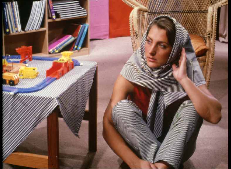
Figure 8: (Color online) Our diffusion constrained total variation scheme (stopping parameter ϵ=104italic-ϵsuperscript104\epsilon=10^{-4}) provides better edge preserving cartoon component u𝑢u when compared to the traditional TV regularization model [9]. Even with constant μ𝜇\mu, λ𝜆\lambda the proposed scheme provides better results (see top row (b)). The crop regions highlight that the proposed scheme provides better preservation of large scale textures compared to [9] model. Best viewed electronically, zoomed in.
Refer to caption
Refer to caption
Refer to caption
Refer to caption
Refer to caption
Refer to caption
Refer to caption
Refer to caption
Refer to caption
Refer to caption
Refer to caption
Refer to caption
Refer to caption
Refer to caption
Refer to caption
Refer to caption
Refer to caption
Refer to caption
Refer to caption
Refer to caption
Figure 9: (Color online) Effect of constant μ𝜇\mu in color image decomposition using our coupled scheme on the cartoon (u𝑢u) component. First row: Original color RGB images. Cartoon component result for constant μ𝜇\mu, λ𝜆\lambda with stopping parameter, Second row: ϵ=104italic-ϵsuperscript104\epsilon=10^{-4}, and Third row: ϵ=106italic-ϵsuperscript106\epsilon=10^{-6}. As can be seen decreasing the stopping parameter removes more texture details and provides piecewise constant cartoon image. Last row: Shows the proposed scheme results with adaptive μ1subscript𝜇1\mu_{1}, see Eqn. (17) and constant λ𝜆\lambda (stopping parameter ϵ=104italic-ϵsuperscript104\epsilon=10^{-4}) . Best viewed electronically, zoomed in.
Refer to caption
Refer to caption
Refer to caption
Refer to caption
Refer to caption
Refer to caption
Refer to caption
Refer to caption
Refer to caption
Refer to caption
Refer to caption
Refer to caption
Refer to caption
Refer to caption
Refer to caption
Figure 10: (Color online) Corresponding texture components v𝑣v. Arrangement is as in Figure 9. Best viewed electronically, zoomed in.
Refer to caption
Refer to caption
Refer to caption
Refer to caption
Refer to caption
Refer to caption
Refer to caption
Refer to caption
Refer to caption
Refer to caption
Refer to caption
Refer to caption
Refer to caption
Refer to caption
Refer to caption
Figure 11: (Color online) Corresponding edge functions w𝑤w. Arrangement is as in Figure 9. Best viewed electronically, zoomed in.

We further provide image decomposition for color images [8, 22] by using vectorial TV version in Eqn. (7) following [8]. We consider the following vectorial TV with non-homogenous diffusion equation:
min𝐮=(u1,u2,u3){Ωg(wi)i=13|ui|𝑑x+i=13Ωμ(x)|uifi|𝑑x},subscript𝐮subscript𝑢1subscript𝑢2subscript𝑢3subscriptΩ𝑔subscript𝑤𝑖superscriptsubscript𝑖13subscript𝑢𝑖differential-d𝑥superscriptsubscript𝑖13subscriptΩ𝜇𝑥subscript𝑢𝑖subscript𝑓𝑖differential-d𝑥\displaystyle\min\limits_{\mathbf{u}=(u_{1},u_{2},u_{3})}\Bigg{\{}\int_{\Omega}g(w_{i})\sqrt{\sum_{i=1}^{3}|\nabla u_{i}|}\,dx+\sum_{i=1}^{3}\int_{\Omega}\mu(x)\,|u_{i}-f_{i}|\,dx\Bigg{\}},
wit=λi(x)div(wi)+(1λi(x))(|ui|wi),subscript𝑤𝑖𝑡subscript𝜆𝑖𝑥𝑑𝑖𝑣subscript𝑤𝑖1subscript𝜆𝑖𝑥subscript𝑢𝑖subscript𝑤𝑖\displaystyle\frac{\partial w_{i}}{\partial t}=\lambda_{i}(x)div(\nabla w_{i})+(1-\lambda_{i}(x))(|\nabla u_{i}|-w_{i}),

were each scalar function ui:Ω:subscript𝑢𝑖Ωu_{i}:\Omega\rightarrow\mathbb{R}, 1i31𝑖31\leq i\leq 3 represent one component of the RGB color system. Note that following our alternating iterative scheme given by equations (10), (12) and (14) the new solutions (ui,vi,wi)subscript𝑢𝑖subscript𝑣𝑖subscript𝑤𝑖(u_{i},v_{i},w_{i}) are given by:

ui=fiviθdiv𝐩i,subscript𝑢𝑖subscript𝑓𝑖subscript𝑣𝑖𝜃𝑑𝑖𝑣subscript𝐩𝑖u_{i}=f_{i}-v_{i}-\theta div\,\mathbf{p}_{i}, (97)

where 𝐩i=(pi1,pi2)subscript𝐩𝑖subscript𝑝subscript𝑖1subscript𝑝subscript𝑖2\mathbf{p}_{i}=(p_{i_{1}},p_{i_{2}}) satisfies g(wi)(θdiv𝐩i(fivi))|(θdiv𝐩i(fivi))|𝐩i=0𝑔subscript𝑤𝑖𝜃divsubscript𝐩𝑖subscript𝑓𝑖subscript𝑣𝑖𝜃divsubscript𝐩𝑖subscript𝑓𝑖subscript𝑣𝑖subscript𝐩𝑖0g(w_{i})\nabla(\theta\,\mathrm{div}\,\mathbf{p}_{i}-(f_{i}-v_{i}))-|\nabla(\theta\mathrm{div}\,\mathbf{p}_{i}-(f_{i}-v_{i}))|\mathbf{p}_{i}=0, which is solved using a fixed point method: 𝐩i0=0subscriptsuperscript𝐩0𝑖0\mathbf{p}^{0}_{i}=0 and

𝐩in+1=𝐩in+δt(div(𝐩in)(fivi)/θ)1+δtg(wi)i=13|(div(𝐩in)(fivi)/θ)|2.subscriptsuperscript𝐩𝑛1𝑖subscriptsuperscript𝐩𝑛𝑖𝛿𝑡divsubscriptsuperscript𝐩𝑛𝑖subscript𝑓𝑖subscript𝑣𝑖𝜃1𝛿𝑡𝑔subscript𝑤𝑖superscriptsubscript𝑖13superscriptdivsubscriptsuperscript𝐩𝑛𝑖subscript𝑓𝑖subscript𝑣𝑖𝜃2\mathbf{p}^{n+1}_{i}=\frac{\mathbf{p}^{n}_{i}+\delta t\nabla(\mathrm{div}(\mathbf{p}^{n}_{i})-(f_{i}-v_{i})/\theta)}{1+\displaystyle\frac{\delta t}{g(w_{i})}\sqrt{\sum_{i=1}^{3}|\nabla(\mathrm{div}(\mathbf{p}^{n}_{i})-(f_{i}-v_{i})/\theta)|^{2}}}.
vi={fiuiθμ(x)if fiuiθμ(x),fiui+θμ(x)if fiuiθμ(x),0if |fiui|θμ(x).subscript𝑣𝑖casessubscript𝑓𝑖subscript𝑢𝑖𝜃𝜇𝑥if fiuiθμ(x)subscript𝑓𝑖subscript𝑢𝑖𝜃𝜇𝑥if fiuiθμ(x)0if |fiui|θμ(x)v_{i}=\begin{cases}f_{i}-u_{i}-\theta\mu(x)&\text{if $f_{i}-u_{i}\geq\theta\mu(x)$},\\ f_{i}-u_{i}+\theta\mu(x)&\text{if $f_{i}-u_{i}\leq-\theta\mu(x)$},\\ 0&\text{if $|f_{i}-u_{i}|\leq\theta\mu(x)$}.\end{cases} (98)
win+1=win+δt(δx)2(λ(x)Δ~win+(1λ(x))(|ui|win)).subscriptsuperscript𝑤𝑛1𝑖subscriptsuperscript𝑤𝑛𝑖𝛿𝑡superscript𝛿𝑥2𝜆𝑥~Δsubscriptsuperscript𝑤𝑛𝑖1𝜆𝑥subscript𝑢𝑖subscriptsuperscript𝑤𝑛𝑖w^{n+1}_{i}=w^{n}_{i}+\frac{\delta t}{(\delta x)^{2}}(\lambda(x)\tilde{\Delta}w^{n}_{i}+(1-\lambda(x))\left(\left|\nabla u_{i}\right|-w^{n}_{i}\right)). (99)
Refer to caption
Refer to caption
Refer to caption
Refer to caption
(a) Input (f𝑓f) and u𝑢u components using the proposed model
Refer to caption
Refer to caption
Refer to caption
(b) (Pseudo) Edges (w𝑤w)
Refer to caption
(c) Canny Edges
Figure 12: (Color online) Pseudo edge maps & Canny Edges. First Row: Input (f𝑓f) and u𝑢u components using the proposed model with (μ𝜇absent\mu\leftarrowadaptive, λ𝜆absent\lambda\leftarrowconstant) and stopping parameter ϵ=104italic-ϵsuperscript104\epsilon=10^{-4}. Second and Third Row: (Pseudo) Edges (w𝑤w) (First Column) and Canny Edges (Second Column).

Figure 8 shows the cartoon components of our CTE scheme with constant and adaptive μ1subscript𝜇1\mu_{1} against the traditional TV based scheme of [9] for two standard RGB test images. As can be seen, our scheme obtains better edge preserving cartoon (u𝑢u) components. The close-up shots indicate that our scheme also avoids blurring of edges, see for example Barbara𝐵𝑎𝑟𝑏𝑎𝑟𝑎Barbara face. See also Figure 3 where the proposed scheme with adaptive μ1subscript𝜇1\mu_{1} provides better shape preservation as stopping parameters increase from ϵ=104italic-ϵsuperscript104\epsilon=10^{-4} to ϵ=107italic-ϵsuperscript107\epsilon=10^{-7}. Next, Figures 9-11 shows decomposition for a variety of RGB images for two different iteration values in our proposed CTE scheme with constant μ𝜇\mu against adaptive μ1subscript𝜇1\mu_{1} based results. As can be seen in Figure 9, increasing the number of iterations removes more texture details and provides piecewise constant (smoother) cartoon images. Our adaptive μ1subscript𝜇1\mu_{1} based scheme results (last row) on the other hand keep most of the salient edges. This can be seen further in Figure 10 (last row) where the adaptive μ1subscript𝜇1\mu_{1} based scheme captures only small scale oscillations corresponding to texture components whereas the constant μ𝜇\mu based results remove strong edges as well. Figure 11 show the corresponding edge functions, and it can be seen that adaptive scheme has more information than in constant parameter case. Thus, we conclude that, using adaptive μ𝜇\mu provides an image adaptive way of obtaining edge preserving cartoon components without sacrificing overall decomposition properties.

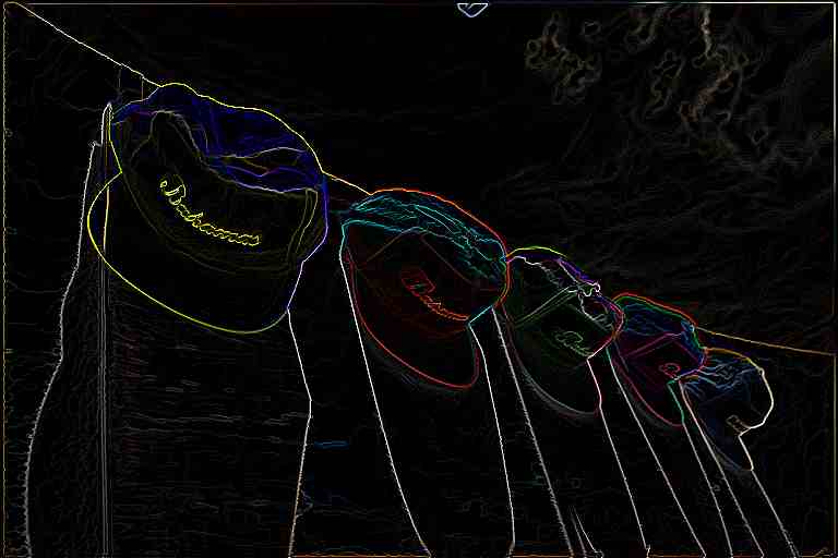
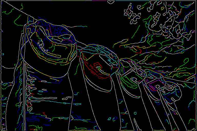
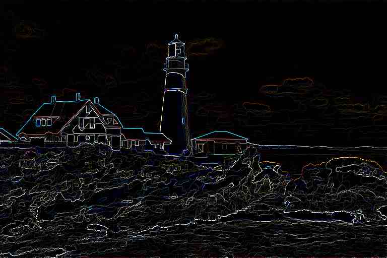
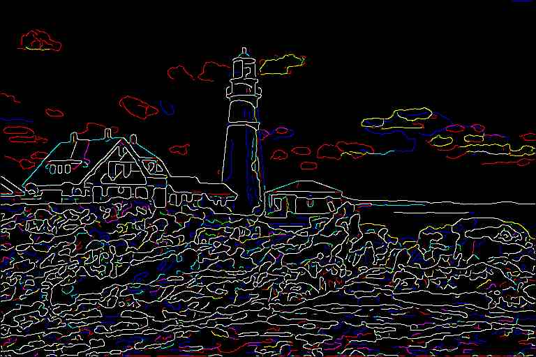
Figure 12 shows the cartoon component of two different color images as well as the edge functions given by the proposed model, and Canny edge maps [11] computed in all the three channels999Computed using the MATLAB’s default command edge(u,‘canny’).. As observed the function w𝑤w captures edges based on the cartoon subregions i.e. large intensity gradients while the Canny edge maps captures large and small intensity gradients.
4.2.3 Comparison with other decomposition methods

Image/MSSIM OSV VC AGO BP CP DHC BCM MCTE ACTE CCTE
Girl1\dagger/0.2081 27.5748 28.1667 28.0247 27.1771 27.9446 28.3862 28.4113 28.8536 28.3557 28.8266
0.7664 0.7669 0.7705 0.7531 0.7604 0.7732 0.7293 0.7971 0.7893 0.7939
Couple1\dagger/0.2029 27.1529 28.3845 27.7122 27.4384 27.8213 28.1447 28.5528 28.5297 28.0973 29.4769
0.6918 0.7080 0.7022 0.7063 0.7042 0.7283 0.7045 0.7467 0.7439 0.7548
Girl2\dagger/0.1482 29.6239 30.6253 29.6591 30.6260 29.7908 32.0758 30.9228 32.2619 30.7951 32.1304
0.8730 0.8039 0.8829 0.8779 0.8751 0.8950 0.7991 0.8964 0.8933 0.8821
Girl3\dagger/0.2261 29.4733 29.3198 28.8185 28.2566 28.7244 30.6547 29.3895 31.3260 29.1061 31.1257
0.8470 0.8029 0.8335 0.8092 0.8145 0.8014 0.7831 0.8469 0.8595 0.8379
House1\dagger/0.2297 27.1664 26.5337 27.7950 27.4868 28.0119 29.2988 29.4386 29.0679 28.4171 29.5162
0.7858 0.7626 0.7831 0.7950 0.7795 0.7993 0.7603 0.8138 0.8090 0.8064
Tree\dagger/0.3959 23.7801 24.4972 24.0548 24.2811 24.3028 26.3365 26.0382 26.9758 24.3702 27.0157
0.7259 0.7549 0.7231 0.7487 0.7314 0.7654 0.7684 0.7702 0.7489 0.7666
Jelly1\dagger/0.1700 29.7350 29.8272 29.4804 30.0963 29.2544 30.6860 30.2663 31.4578 31.2529 30.9478
0.9181 0.8297 0.9351 0.9153 0.9178 0.9360 0.8407 0.9369 0.9376 0.9145
Jelly2\dagger/0.2294 28.8000 28.9457 27.5507 28.1674 27.9968 29.1260 29.2134 30.0485 29.5462 29.9156
0.9098 0.8385 0.9029 0.8923 0.9005 0.8227 0.8443 0.9202 0.9182 0.9020
Splash\ddagger/0.4151 30.6488 28.9810 29.9935 31.4922 31.2080 33.1049 31.0800 33.8236 31.3856 31.2644
0.8825 0.8312 0.8891 0.8818 0.8740 0.8669 0.8732 0.8975 0.8935 0.9020
Tiffany\ddagger/0.4482 29.2555 28.0636 28.6905 30.2667 29.7630 31.2730 29.6920 32.0779 30.7028 31.3727
0.8617 0.8254 0.8534 0.8425 0.8491 0.8567 0.8628 0.8708 0.8612 0.8685
Mandril\ddagger/0.7097 20.4765 21.6728 20.7883 21.9056 20.9060 23.7888 23.9897 23.7899 20.8689 22.3085
0.65255 0.7651 0.6443 0.6962 0.6530 0.8002 0.8247 0.8117 0.6520 0.7713
Table 1: PSNR (dB) and MSSIM comparison of various decomposition schemes with noise level σ=30𝜎30\sigma=30 for standard test images from the USC-SIPI database with size =256×256\dagger=256\times 256 (Noisy PSNR=22.11PSNR22.11\text{PSNR}=22.11) and =512×512\ddagger=512\times 512 (Noisy PSNR=22.09PSNR22.09\text{PSNR}=22.09). Each row indicates PSNR/MSSIM values for different test images. The diffusion with multiscale (μ𝜇absent\mu\leftarrowmultiscale, λ𝜆absent\lambda\leftarrowconstant), adaptive choice (μ𝜇absent\mu\leftarrowadaptive, λ𝜆absent\lambda\leftarrowconstant) and constant CTE scheme (μ𝜇absent\mu\leftarrowconstant, λ𝜆absent\lambda\leftarrowconstant) are given as MCTE, ACTE and CCTE (last three columns) respectively (stopping parameter ϵ=104italic-ϵsuperscript104\epsilon=10^{-4}). Compared methods are OSV [40], VC [55], AGO [6], BP [7], CP [15], DHC [20], BCM [10]. Best results are indicated in boldface and the second best is underlined.

.

Refer to caption
(a) Barbara𝐵𝑎𝑟𝑏𝑎𝑟𝑎Barbara image
Refer to caption
(b) Canny edges
Refer to caption
(c) Noisy Barbara𝐵𝑎𝑟𝑏𝑎𝑟𝑎Barbara
Refer to caption
(d) Canny edges
Refer to caption
(e) Input noise
Refer to captionRefer to captionRefer to captionRefer to captionRefer to captionRefer to caption(b) u & fu for VC [55](c) u & fu for OSV [40](d) u & fu for AGO [6]Refer to captionRefer to captionRefer to captionRefer to captionRefer to captionRefer to caption(b) u & fu for VC [55](c) u & fu for OSV [40](d) u & fu for AGO [6]\begin{array}[]{ccc}\includegraphics[width=71.13188pt,height=78.24507pt]{barbara_TVpmodelDeno30_u}\includegraphics[width=71.13188pt,height=78.24507pt]{barbara_TVpmodelDeno30_residuo}&\includegraphics[width=71.13188pt,height=78.24507pt]{barbara_TVH1Deno30_u}\includegraphics[width=71.13188pt,height=78.24507pt]{barbara_TVH1Deno30_residuo}&\includegraphics[width=71.13188pt,height=78.24507pt]{barbara_TVGarborDeno30_u}\includegraphics[width=71.13188pt,height=78.24507pt]{barbara_TVGarborDeno30_residuo}\\ \mbox{\scriptsize{(b) $u$ \& $f-u$ for VC~{}\cite[cite]{[\@@bibref{}{VChan04}{}{}]}}}&\mbox{\scriptsize{(c) $u$ \& $f-u$ for OSV~{}\cite[cite]{[\@@bibref{}{OSVese03}{}{}]}}}&\mbox{\scriptsize{(d) $u$ \& $f-u$ for AGO~{}\cite[cite]{[\@@bibref{}{AujolGilboa06}{}{}]}}}\end{array}
Refer to caption
Refer to caption
Refer to caption
Refer to caption
Refer to caption
Refer to caption
Refer to caption
Refer to caption
Refer to caption
Refer to caption
Refer to caption
Refer to caption
Refer to caption
Refer to caption
Refer to caption
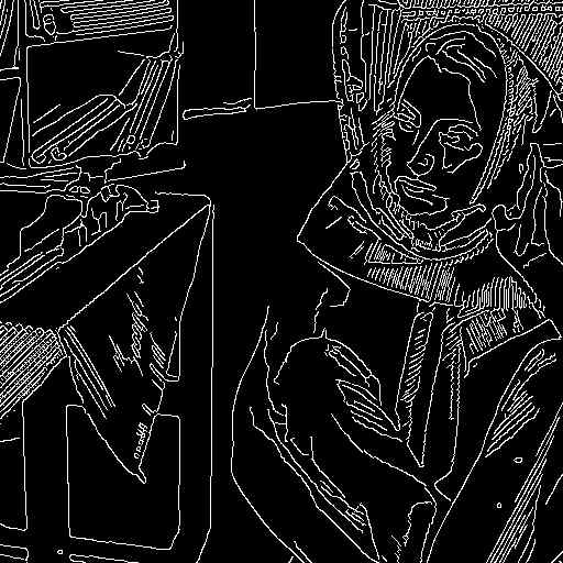
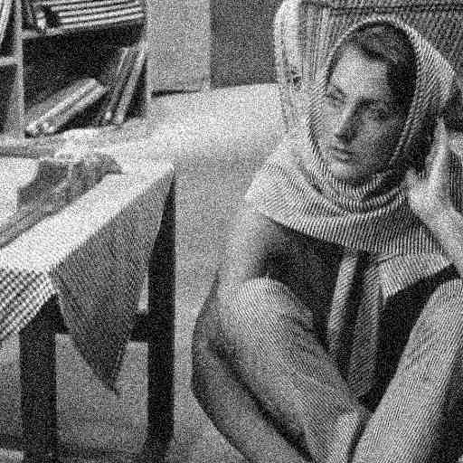
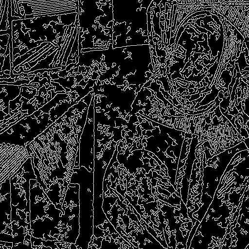
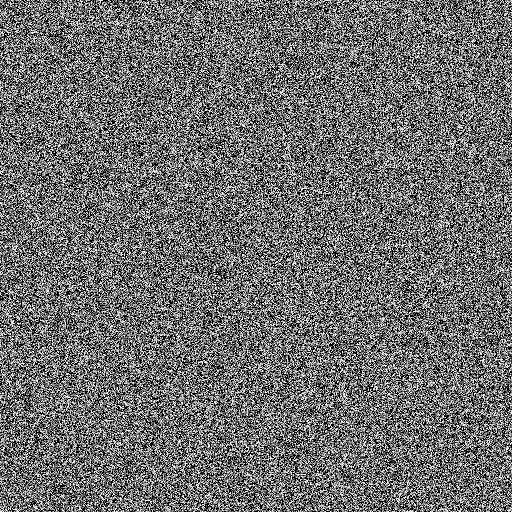
(e) u,v,w𝑢𝑣𝑤u,v,w, fu𝑓𝑢f-u, and f(u+v+w)𝑓𝑢𝑣𝑤f-(u+v+w) components for the proposed scheme.
Figure 13: Decomposition of noise inputs. (a) House𝐻𝑜𝑢𝑠𝑒House, F16𝐹16F-16 and Barbara𝐵𝑎𝑟𝑏𝑎𝑟𝑎Barbara images corrupted by Gaussian noise images (standard deviation σ=30𝜎30\sigma=30). (b)-(d) u𝑢u & fu𝑓𝑢f-u components provided by the VC [55], OSV [40] and AGO [6] schemes, respectively. (e) u,v,w,fu𝑢𝑣𝑤𝑓𝑢u,v,w,f-u and f(u+v+w)𝑓𝑢𝑣𝑤f-(u+v+w) components using the proposed CTE scheme with (CCTE - μ𝜇absent\mu\leftarrowconstant, λ𝜆absent\lambda\leftarrowconstant) for the Third row, with (ACTE - μ𝜇absent\mu\leftarrowadaptive, λ𝜆absent\lambda\leftarrowconstant) for the Fourth row and (MCTE - μ𝜇absent\mu\leftarrowmultiscale, λ𝜆absent\lambda\leftarrow) for the Fifth row. The corresponding PSNR (dB) and MSSIM measures for each model are displayed in Table 1.

.

Next we use the grayscale digitize images from USC-SIPI Image Database to compare the performance of the CTE model together with the adaptive and multi-scale case with the following schemes: TV-H1superscript𝐻1H^{-1} decomposition model (OSV, using finite differences) [40], TV-Gpsubscript𝐺𝑝G_{p} decomposition model (VC, finite differences channel-wise) [55], TV-Garbor𝐺𝑎𝑟𝑏𝑜𝑟Garbor decomposition model (AGO, Chambolle’s projection algorithm ) [6], BV2L2𝐵superscript𝑉2superscript𝐿2BV^{2}-L^{2} model (BP, which uses an algorithm close to the one set by dual minimization of [14] and  [55][7], TVL1𝑇𝑉superscript𝐿1TV-L^{1} model (CP, a first-order primal-dual algorithm) [15], Lτsuperscript𝐿𝜏L^{\tau}-TV𝑇𝑉TV scheme for color images (DHC, using a unified Moreau-Yosida based primal-dual approach) [20], and the NL- Means algorithm (BCM, a improvement of the classical and state-of-the-art methods in image denosing) [10] which computes the local average color of the most resembling pixels using non-local means.
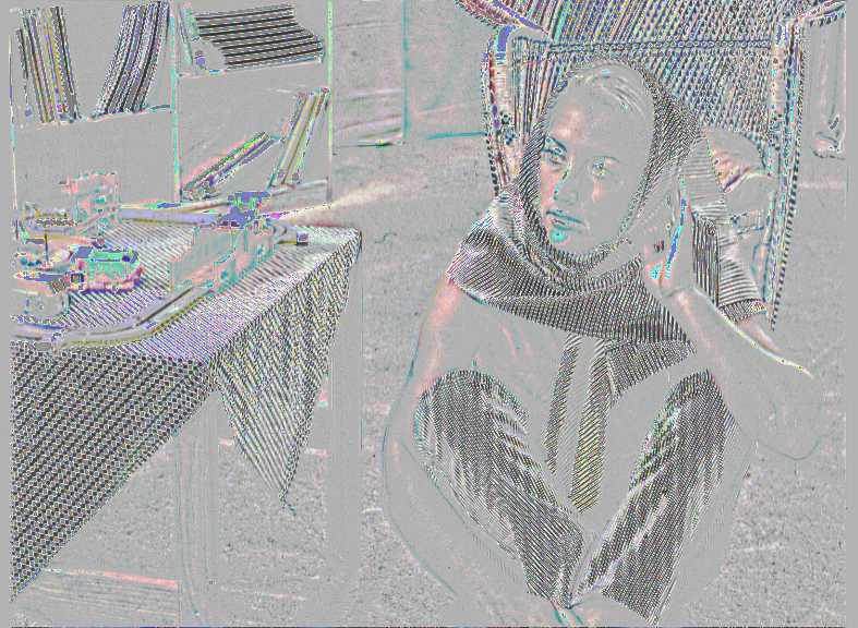
Numerical results are given in Table 1 for sixteen standard natural grayscale images of size 256×256256256256\times 256 and 512×512512512512\times 512. As we can see the proposed scheme based on multi-scale lambda (μ𝜇absent\mu\leftarrowmultiscale, λ𝜆absent\lambda\leftarrowconstant) and the adaptive choice (μ𝜇absent\mu\leftarrowmultiscale, λ𝜆absent\lambda\leftarrowconstant) performs well for a variety of images. Even with the adaptive choice (ACTE, μ𝜇absent\mu\leftarrowadaptive, λ𝜆absent\lambda\leftarrowconstant) outperforms previous variational models bases H1superscript𝐻1H^{-1}, Gpsubscript𝐺𝑝G_{p} and Garbor𝐺𝑎𝑟𝑏𝑜𝑟Garbor norms and in some cases the Lτsuperscript𝐿𝜏L^{\tau}-TV𝑇𝑉TV and the NL-Means schemes. For textured images such as Mandrill𝑀𝑎𝑛𝑑𝑟𝑖𝑙𝑙Mandrill and Barbara𝐵𝑎𝑟𝑏𝑎𝑟𝑎Barbara we perform all variational models except the NL-means algorithm. We remark that the proposed CTE model does not aim to give state-of-the-art results for image denoising, and instead concentrates on demonstrating how our decomposition model can be harnessed for noise removal and edge detention. Figure 13 shows decomposition for Barbara𝐵𝑎𝑟𝑏𝑎𝑟𝑎Barbara into different components for some of the schemes in Table 1. We note that for other schemes we are able to discompose the image in u𝑢u (smooth) and fu𝑓𝑢f-u (random noise). In our case, we are able to obtain edge variable w𝑤w component. We also notice that for our model the random noise component fu𝑓𝑢f-u is directly given by the v𝑣v component.

4.3 Image denoising results

4.3.1 Error metrics

Currently there are no quantitative ways to evaluate different decomposition algorithms. In particular which smooth, texture and edge separation model are better is an open research question in image quality assessment. The proposed decomposition provides piecewise cartoon component which is obtained using a weighted TV regularization in an edge preserving way, see Figure 9 (last row). Hence, as a byproduct we obtain image denoising, with u𝑢u the denoised image and v+w𝑣𝑤v+w the ‘noise’ part. To compare the schemes quantitatively for the purpose of denoising, we utilize two commonly used error metrics in the image denoising literature, one is the classical peak signal to noise ratio (PSNR) [3], and the other one is the mean structural similarity measure (MSSIM) [57].

  1. 1.

    PSNR is given in decibels (dB𝑑𝐵dB). A difference of 0.5dB0.5𝑑𝐵0.5\,dB can be identified visually. Higher PSNR value indicates optimum denoising capability.

    PSNR(u):=20log10(umaxMSE)dB,assignPSNR𝑢2010subscript𝑢𝑚𝑎𝑥𝑀𝑆𝐸𝑑𝐵\displaystyle\text{PSNR}(u):=20*\log 10{\left(\frac{u_{max}}{\sqrt{MSE}}\right)}\,dB, (100)

    where MSE=(mn)1(uu0)MSEsuperscript𝑚𝑛1𝑢subscript𝑢0\text{MSE}=(mn)^{-1}\sum\sum(u-u_{0}), m×n𝑚𝑛m\times n denotes the image size, umaxsubscript𝑢𝑚𝑎𝑥u_{max} denotes the maximum value, for example in 888-bit images umax=255subscript𝑢𝑚𝑎𝑥255u_{max}=255.

  2. 2.

    MSSIM index is in the range [0,1]01[0,1]. The MSSIM value near one implies the optimal denoising capability of the scheme [57] and is mean value of the SSIM metric. The SSIM is calculated between two windows ω1subscript𝜔1\omega_{1} and ω2subscript𝜔2\omega_{2} of common size N×N𝑁𝑁N\times N,

    SSIM(ω1,ω2)=(2μω1μω2+c1)(2σω1ω2+c2)(μω12+μω22+c1)(σω12+σω22+c2),SSIMsubscript𝜔1subscript𝜔22subscript𝜇subscript𝜔1subscript𝜇subscript𝜔2subscript𝑐12subscript𝜎subscript𝜔1subscript𝜔2subscript𝑐2superscriptsubscript𝜇subscript𝜔12superscriptsubscript𝜇subscript𝜔22subscript𝑐1superscriptsubscript𝜎subscript𝜔12superscriptsubscript𝜎subscript𝜔22subscript𝑐2\displaystyle\text{SSIM}(\omega_{1},\omega_{2})=\frac{(2\mu_{\omega_{1}}\mu_{\omega_{2}}+c_{1})(2\sigma_{\omega_{1}\omega_{2}}+c_{2})}{(\mu_{\omega_{1}}^{2}+\mu_{\omega_{2}}^{2}+c_{1})(\sigma_{\omega_{1}}^{2}+\sigma_{\omega_{2}}^{2}+c_{2})},

    where μωisubscript𝜇subscript𝜔𝑖\mu_{\omega_{i}} the average of ωisubscript𝜔𝑖\omega_{i}, σωi2subscriptsuperscript𝜎2subscript𝜔𝑖\sigma^{2}_{\omega_{i}} the variance of ωisubscript𝜔𝑖\omega_{i}, σω1ω2subscript𝜎subscript𝜔1subscript𝜔2\sigma_{\omega_{1}\omega_{2}} the covariance, c1,c2subscript𝑐1subscript𝑐2c_{1},c_{2} stabilization parameters, see [57] for more details.

Remark 4.

Note that the SSIM is a better error metric than PSNR as it provides a quantitative way of measuring the structural similarity of denoised image against the original noise-free image. To adapt PSNR and SSIM error metrics to color images one can convert the color image into gray101010For example, using MATLAB’s command rgb2gray. and then compute PSNR and MSSIM error metrics for the converted gray-scale image. In this paper, in order to compare with the scheme on [48], we compute the PSNR and MSSIM on each channel and use the average as a final value.
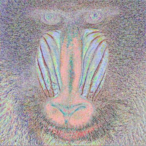
4.3.2 Comparison with the previous model

Table 2 compares proposed scheme with that of [48] using the both PSNR (dB) and MSSIM error metrics average for Berkeley segmentation dataset (BSDS) images. We implemented both the schemes on the full Berkeley segmentation dataset of 500500500 noisy images for two different noise levels and obtained similar improvements. Figures 14-15 show some example images corresponding to Table 2. As can be seen from the zoomed in versions, the proposed CTE scheme provides cleaner cartoon components (denoised images, see Figures 14(b-e)-15(b,c)) in contrast to original coupled PDE model [48] which either excessively blurs out details (Figure 14(f,g)) or keeps noisy regions (Figure 15(d)) in final results.
Refer to caption
Refer to caption
(a) Input noise (σ=20𝜎20\sigma=20), (PSNR,MSSIM)=(24.1759,0.5130)PSNRMSSIM24.17590.5130(\mbox{PSNR},\mbox{MSSIM})=(24.1759,0.5130)
Refer to captionRefer to captionRefer to captionRefer to caption(b) Proposed (μadaptive, λconstant ) (c) Proposed (μadaptive, λconstant) (PSNR,MSSIM)=(28.6484,0.7675)(PSNR,MSSIM)=(27.5146,0.6993)Refer to captionRefer to captionRefer to captionRefer to caption(d) Proposed (μconstant, λadaptive ) (e) Proposed (μconstant, λadaptive) (PSNR,MSSIM)=(27.6574,0.7285)(PSNR,MSSIM)=(26.8005,0.6849)Refer to captionRefer to captionRefer to captionRefer to caption(f) [48] (Adaptive)(g) [48] (Adaptive)(PSNR,MSSIM)=(26.1172,0.7540)(PSNR,MSSIM)=(24.8883,0.7057)Refer to captionRefer to captionRefer to captionRefer to caption(b) Proposed (μadaptive, λconstant ) (c) Proposed (μadaptive, λconstant) PSNRMSSIM28.64840.7675PSNRMSSIM27.51460.6993Refer to captionRefer to captionRefer to captionRefer to caption(d) Proposed (μconstant, λadaptive ) (e) Proposed (μconstant, λadaptive) PSNRMSSIM27.65740.7285PSNRMSSIM26.80050.6849Refer to captionRefer to captionRefer to captionRefer to caption(f) [48] (Adaptive)(g) [48] (Adaptive)PSNRMSSIM26.11720.7540PSNRMSSIM24.88830.7057\begin{array}[]{cc}\includegraphics[width=119.50148pt,height=99.58464pt]{Berkeley_CTE_20_1_images_u_108005}\includegraphics[width=99.58464pt,height=99.58464pt]{Berkeley_CTE_20_1_images_u_108005Face}&\includegraphics[width=119.50148pt,height=99.58464pt]{Berkeley_CTE_20_2_images_u_108005}\includegraphics[width=99.58464pt,height=99.58464pt]{Berkeley_CTE_20_2_images_u_108005Face}\\ \mbox{\scriptsize{(b) Proposed ($\mu\leftarrow$adaptive, $\lambda\leftarrow$constant ) }}&\mbox{\scriptsize{(c) Proposed ($\mu\leftarrow$adaptive, $\lambda\leftarrow$constant) }}\\ \mbox{\scriptsize{$(\mbox{PSNR},\mbox{MSSIM})=(28.6484,0.7675)$}}&\mbox{\scriptsize{$(\mbox{PSNR},\mbox{MSSIM})=(27.5146,0.6993)$}}\\ \includegraphics[width=119.50148pt,height=99.58464pt]{Berkeley_CTE_20_1_images_u_108005_mucons_lambadap}\includegraphics[width=99.58464pt,height=99.58464pt]{Berkeley_CTE_20_1_images_u_108005Face_mucons_lambadap}&\includegraphics[width=119.50148pt,height=99.58464pt]{Berkeley_CTE_20_2_images_u_108005_mucons_lambadap}\includegraphics[width=99.58464pt,height=99.58464pt]{Berkeley_CTE_20_2_images_u_108005Face_mucons_lambadap}\\ \mbox{\scriptsize{(d) Proposed ($\mu\leftarrow$constant, $\lambda\leftarrow$adaptive ) }}&\mbox{\scriptsize{(e) Proposed ($\mu\leftarrow$constant, $\lambda\leftarrow$adaptive) }}\\ \mbox{\scriptsize{$(\mbox{PSNR},\mbox{MSSIM})=(27.6574,0.7285)$}}&\mbox{\scriptsize{$(\mbox{PSNR},\mbox{MSSIM})=(26.8005,0.6849)$}}\\ \includegraphics[width=119.50148pt,height=99.58464pt]{Berkeley_coupled_VBS_20_3_images_u_108005}\includegraphics[width=99.58464pt,height=99.58464pt]{Berkeley_coupled_VBS_20_3_images_u_108005Face}&\includegraphics[width=119.50148pt,height=99.58464pt]{Berkeley_coupled_VBS_20_1_images_u_108005}\includegraphics[width=99.58464pt,height=99.58464pt]{Berkeley_coupled_VBS_20_1_images_u_108005Face}\\ \mbox{\scriptsize{(f) ~{}\cite[cite]{[\@@bibref{}{PVorotnikov12}{}{}]} (Adaptive)}}&\mbox{\scriptsize{(g) ~{}\cite[cite]{[\@@bibref{}{PVorotnikov12}{}{}]}} (Adaptive)}\\ \mbox{\scriptsize{$(\mbox{PSNR},\mbox{MSSIM})=(26.1172,0.7540)$}}&\mbox{\scriptsize{$(\mbox{PSNR},\mbox{MSSIM})=(24.8883,0.7057)$}}\\ \end{array}
Figure 14: (Color online) Better edge preserving image restoration results were obtained using our scheme in comparison with the original coupled PDE model [48]. The stopping parameters were chosen according to maximum MSSIM values, see Table 2 for the corresponding values.
Refer to captionRefer to captionRefer to captionRefer to caption(a) Input noise (σ=30), (PSNR,MSSIM)=(21.888,0.2445)(b) Proposed (μadaptive, λconstant) (PSNR,MSSIM)=(28.3610,0.7718)Refer to captionRefer to captionRefer to captionRefer to caption(c) Proposed (μconstant, λadaptive) (d) [48] (μconstant, λadaptive)(PSNR,MSSIM)=(29.2489,0.7636)(PSNR,MSSIM)=(26.4529,0.6849)Refer to captionRefer to captionRefer to captionRefer to caption(a) Input noise (σ=30), (PSNR,MSSIM)=(21.888,0.2445)(b) Proposed (μadaptive, λconstant) missing-subexpressionPSNRMSSIM28.36100.7718Refer to captionRefer to captionRefer to captionRefer to caption(c) Proposed (μconstant, λadaptive) (d) [48] (μconstant, λadaptive)PSNRMSSIM29.24890.7636PSNRMSSIM26.45290.6849\begin{array}[]{cc}\includegraphics[width=108.12054pt,height=113.81102pt]{Berkeley_CTE_30_2_images_noisy_101087}\includegraphics[width=108.12054pt,height=113.81102pt]{Berkeley_CTE_30_2_images_noisy_101087Face}&\includegraphics[width=108.12054pt,height=113.81102pt]{Berkeley_CTE_30_2_images_u_101087}\includegraphics[width=108.12054pt,height=113.81102pt]{Berkeley_CTE_30_2_images_u_101087Face}\\ \mbox{\scriptsize{(a) Input noise ($\sigma=30$), $(\mbox{PSNR},\mbox{MSSIM})=(21.888,0.2445)$}}&\mbox{\scriptsize{(b) Proposed ($\mu\leftarrow$adaptive, $\lambda\leftarrow$constant) }}\\ &\mbox{\scriptsize{$(\mbox{PSNR},\mbox{MSSIM})=(28.3610,0.7718)$}}\\ \includegraphics[width=108.12054pt,height=113.81102pt]{Berkeley_CTE_30_1_images_u_101087_mucons_lambadap}\includegraphics[width=108.12054pt,height=113.81102pt]{Berkeley_CTE_30_1_images_u_101087Face_mucons_lambadap}&\includegraphics[width=108.12054pt,height=113.81102pt]{Berkeley_Coupled_VBS_30_2_images_u_101087}\includegraphics[width=108.12054pt,height=113.81102pt]{Berkeley_Coupled_VBS_30_2_images_u_101087Face}\\ \mbox{\scriptsize{(c) Proposed ($\mu\leftarrow$constant, $\lambda\leftarrow$adaptive) }}&\mbox{\scriptsize{(d)~{}\cite[cite]{[\@@bibref{}{PVorotnikov12}{}{}]} ($\mu\leftarrow$constant, $\lambda\leftarrow$adaptive)}}\\ \mbox{\scriptsize{$(\mbox{PSNR},\mbox{MSSIM})=(29.2489,0.7636)$}}&\mbox{\scriptsize{$(\mbox{PSNR},\mbox{MSSIM})=(26.4529,0.6849)$}}\\ \end{array}
Figure 15: (Color online) Better edge preserving image restoration results were obtained using our scheme in comparison with the original coupled PDE model [48]. The stopping parameters were chosen according to maximum MSSIM values, see Table 2 for the corresponding values.
Method μ𝜇absent\mu\leftarrowconstant μ𝜇absent\mu\leftarrowadaptive Figure Noise Stopping Convergence PSNR (dB)/MSSIM
λ𝜆absent\lambda\leftarrow adaptive λ𝜆absent\lambda\leftarrow constant Example Level Parameter Time(s)
CTE (Proposed) square-root\surd  14 (b) σ=20𝜎20\sigma=20 ϵ=104italic-ϵsuperscript104\epsilon=10^{-4} 30.47 28.7938/0.7723
 14 (c) σ=20𝜎20\sigma=20 ϵ=106italic-ϵsuperscript106\epsilon=10^{-6} 38.71 27.3510/0.7147
 15 (b) σ=30𝜎30\sigma=30 ϵ=106italic-ϵsuperscript106\epsilon=10^{-6} 38.61 26.5238/0.6774
CTE (Proposed) square-root\surd  14 (d) σ=20𝜎20\sigma=20 ϵ=104italic-ϵsuperscript104\epsilon=10^{-4} 30.96 28.2464/0.7237
 14 (e) σ=20𝜎20\sigma=20 ϵ=106italic-ϵsuperscript106\epsilon=10^{-6} 32.20 26.1983/0.6796
 15 (c) σ=30𝜎30\sigma=30 ϵ=106italic-ϵsuperscript106\epsilon=10^{-6} 32.33 26.7451/0.6792
[48] square-root\surd   14 (f) σ=20𝜎20\sigma=20 ϵ=104italic-ϵsuperscript104\epsilon=10^{-4} 5.07 27.3646/0.7178
  14 (g) σ=20𝜎20\sigma=20 ϵ=106italic-ϵsuperscript106\epsilon=10^{-6} 40.57 25.4476/0.6970
 15 (d) σ=30𝜎30\sigma=30 ϵ=106italic-ϵsuperscript106\epsilon=10^{-6} 40.30 25.0559/0.6543
Table 2: Image denoising error metrics (average) comparison using original coupled PDE scheme [48] for different noise levels and parameters on the Berkeley segmentation dataset (BSDS) 500500500. Some examples corresponding to the entries are shown above in Figure 14 and Figure 15.

4.3.3 Comparison of adaptive fidelity parameters

Refer to captionRefer to caption(a) Input noise (σ=20)(b) Energy vs Iteration for different μ choicesRefer to captionRefer to caption(a) Input noise (σ=20)(b) Energy vs Iteration for different μ choices\begin{array}[]{cc}\begin{minipage}[l]{142.26378pt} \includegraphics[width=96.73918pt,height=85.35826pt]{kodim07_no20_crop} \end{minipage}&\begin{minipage}[l]{142.26378pt} \includegraphics[width=184.9429pt,height=142.26378pt]{Lambda_Comparison_lambda_comparisons_kodim07_energy} \end{minipage}\\ \mbox{\footnotesize{(a) Input noise ($\sigma=20$)}}&\hskip 56.9055pt\mbox{\footnotesize{(b) Energy vs Iteration for different $\mu$ choices}}\end{array}
(b) u,v,w,fu components for our proposed scheme using μ1 with (PSNR,MSSIM)=(27.6623,0.8143)Refer to captionRefer to captionRefer to captionRefer to caption(c) u,v,w,fu components for our proposed scheme using μ2 with (PSNR,MSSIM)=(24.6084,0.6823)Refer to captionRefer to captionRefer to captionRefer to caption(d) u,v,w,fu components for our proposed scheme using μ3 with (PSNR,MSSIM)=(25.6414,0.7503)Refer to captionRefer to captionRefer to captionRefer to caption(b) u,v,w,fu components for our proposed scheme using μ1 with (PSNR,MSSIM)=(27.6623,0.8143)Refer to captionRefer to captionRefer to captionRefer to caption(c) u,v,w,fu components for our proposed scheme using μ2 with (PSNR,MSSIM)=(24.6084,0.6823)Refer to captionRefer to captionRefer to captionRefer to caption(d) u,v,w,fu components for our proposed scheme using μ3 with (PSNR,MSSIM)=(25.6414,0.7503)Refer to captionRefer to captionRefer to captionRefer to caption\begin{array}[]{c}\mbox{\scriptsize{(b) $u,v,w,f-u$ components for our proposed scheme using $\mu_{1}$ with \mbox{$(\mbox{PSNR},\mbox{MSSIM})=(27.6623,0.8143)$}}}\\ \includegraphics[width=110.96556pt,height=99.58464pt]{Lambda_comparisons_kodim07_u_CTE}\includegraphics[width=110.96556pt,height=99.58464pt]{Lambda_comparisons_kodim07_v_CTE}\includegraphics[width=110.96556pt,height=99.58464pt]{Lambda_comparisons_kodim07_w_CTE}\includegraphics[width=110.96556pt,height=99.58464pt]{Lambda_comparisons_kodim07_residuo_CTE}\\ \mbox{\scriptsize{(c) $u,v,w,f-u$ components for our proposed scheme using $\mu_{2}$ with \mbox{$(\mbox{PSNR},\mbox{MSSIM})=(24.6084,0.6823)$}}}\\ \includegraphics[width=110.96556pt,height=99.58464pt]{Lambda_comparisons_kodim07_u_Surya}\includegraphics[width=110.96556pt,height=99.58464pt]{Lambda_comparisons_kodim07_v_Surya}\includegraphics[width=110.96556pt,height=99.58464pt]{Lambda_comparisons_kodim07_w_Surya}\includegraphics[width=110.96556pt,height=99.58464pt]{Lambda_comparisons_kodim07_residuo_Surya}\\ \mbox{\scriptsize{(d) $u,v,w,f-u$ components for our proposed scheme using $\mu_{3}$ with \mbox{$(\mbox{PSNR},\mbox{MSSIM})=(25.6414,0.7503)$}}}\\ \includegraphics[width=110.96556pt,height=99.58464pt]{Lambda_comparisons_kodim07_u_IPOL}\includegraphics[width=110.96556pt,height=99.58464pt]{Lambda_comparisons_kodim07_v_IPOL}\includegraphics[width=110.96556pt,height=99.58464pt]{Lambda_comparisons_kodim07_w_IPOL}\includegraphics[width=110.96556pt,height=99.58464pt]{Lambda_comparisons_kodim07_residuo_IPOL}\\ \end{array}
Figure 16: Comparison of different μ𝜇\mu functions computed using a real image corrupted with Gaussian noise level σ=20𝜎20\sigma=20 and stopping parameter ϵ=104italic-ϵsuperscript104\epsilon=10^{-4}. (a) Original image. (b) Energy versus iteration for different adaptive μ𝜇\mu functions based energy minimization scheme (7-8). (c) μ1subscript𝜇1\mu_{1} based on local histograms Eqn. (17). (d) μ2subscript𝜇2\mu_{2} based on the work of [48] Eqn. (18). (e) μ3subscript𝜇3\mu_{3} base on the work of [30] Eqn. (19).

Figure 16 gives a comparison for the implementation of our CTE model (μ𝜇absent\mu\leftarrowadaptive, λ𝜆absent\lambda\leftarrowconstant) by using adaptive fidelity parameters μ1subscript𝜇1\mu_{1} (proposed), μ2subscript𝜇2\mu_{2} (based on the work of [48]) and μ3subscript𝜇3\mu_{3} (studied in [30]) for a close-up flower𝑓𝑙𝑜𝑤𝑒𝑟flower image corrupted with Gaussian noise level σ=20𝜎20\sigma=20. As shown different decomposition levels based on smooth + random noise + edges components are given according to the adaptive parameter μ𝜇\mu. In terms of PSNR and MSSIM error metrics the μ1subscript𝜇1\mu_{1} choice improves better the denoising result. Note the similar convergence property of the energy value between our μ1subscript𝜇1\mu_{1} choice and the μ3subscript𝜇3\mu_{3} adaptive parameter.

4.3.4 Brain MRI image decomposition

Refer to caption
Refer to caption
Refer to caption
Refer to caption
Refer to caption
Refer to caption
(a) Noisy brain MRI images
Refer to caption
Refer to caption
Refer to caption
Refer to caption
Refer to caption
Refer to caption
(b) Cartoon components (u𝑢u)
Refer to caption
Refer to caption
Refer to caption
(c) Edges components (w𝑤w)
Figure 17: (Color online) u𝑢u & w𝑤w components using our proposed model with (μ𝜇absent\mu\leftarrowadaptive, λ𝜆absent\lambda\leftarrowconstant) and stopping parameter ϵ=104italic-ϵsuperscript104\epsilon=10^{-4} for different Brain MR images (slice: 505050, 707070 and 120120120 respectively).
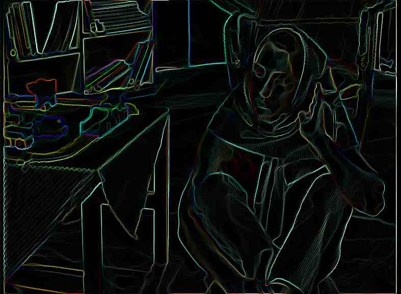
Figure 17 shows input Brain MR images from the Simulated Brain Database and its corresponding (u,v,w)𝑢𝑣𝑤(u,v,w) functions for slices 505050, 707070 and 120120120 together with their corresponding inputs. Lack of sharp edges in the denoised Brain MRI images (Third-Fourth rows) can be attributed to the spatial relaxation based for the coupling PDE scheme. Spatial smoothing based regularization introduces a slight blur on each edge map w𝑤w (Fifth row). Although, we gradually reduce the smoothing results by varying the stopping parameter ϵitalic-ϵ\epsilon the strong discontinuities are preserved well and noise is removed effectively within regions.
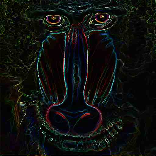
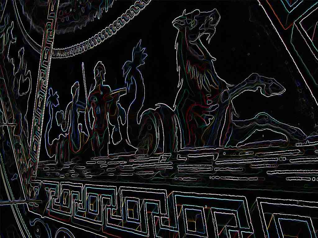
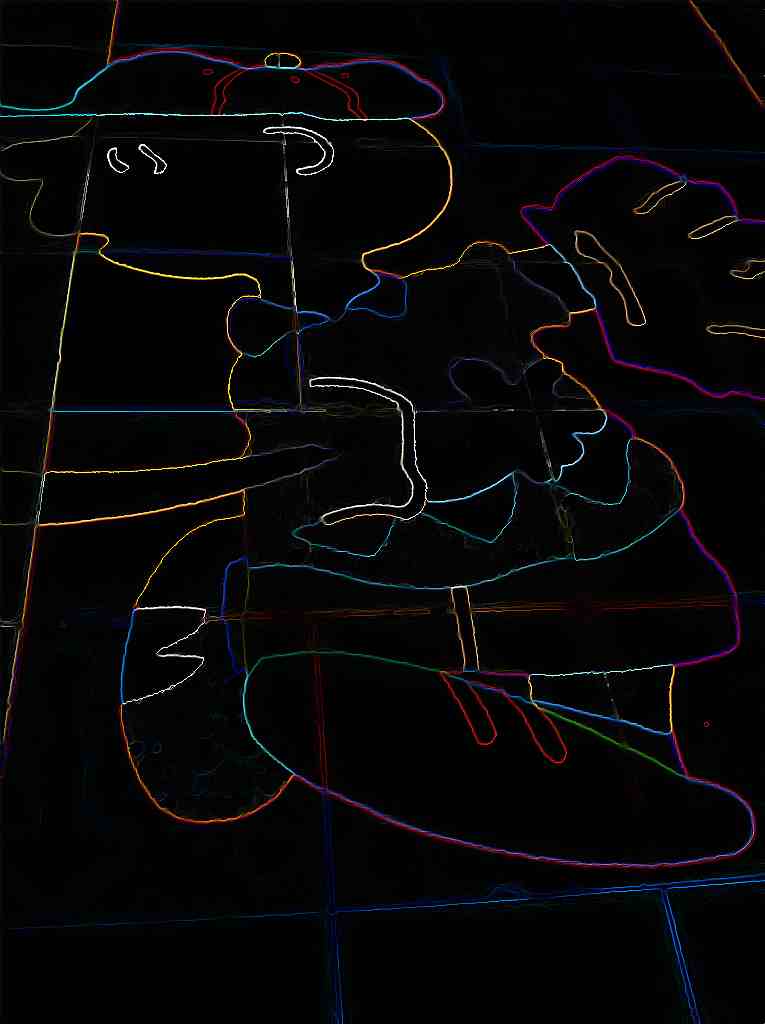
4.4 Multi-scale decomposition

Multiscale cartoon and texture extraction using our proposed CTE methodMultiscale cartoon and texture extraction using our proposed CTE method\begin{array}[]{c}\mbox{\scriptsize{Multiscale cartoon and texture extraction using our proposed CTE method}}\end{array}
Refer to captionRefer to captionRefer to captionRefer to captionRefer to caption(a) u0(b) i=01ui(c) i=02ui(d) i=03ui(f) i=04uiRefer to captionRefer to captionRefer to captionRefer to captionRefer to caption(a) v0(b) i=01vi(c) i=02vi(d) i=03vi(f) i=04viRefer to captionRefer to captionRefer to captionRefer to captionRefer to caption(a) u0(b) i=01ui(c) i=02ui(d) i=03ui(f) i=04uiRefer to captionRefer to captionRefer to captionRefer to captionRefer to caption(a) v0(b) i=01vi(c) i=02vi(d) i=03vi(f) i=04vi\begin{array}[]{ccccc}\includegraphics[width=78.24507pt,height=78.24507pt]{multiscale_comparisons_nat3_resu_CTE_0}&\includegraphics[width=78.24507pt,height=78.24507pt]{multiscale_comparisons_nat3_resu_CTE_1}&\includegraphics[width=78.24507pt,height=78.24507pt]{multiscale_comparisons_nat3_resu_CTE_2}&\includegraphics[width=78.24507pt,height=78.24507pt]{multiscale_comparisons_nat3_resu_CTE_3}&\includegraphics[width=78.24507pt,height=78.24507pt]{multiscale_comparisons_nat3_resu_CTE_4}\\ \mbox{\scriptsize{(a) $u_{0}$}}&\mbox{\scriptsize{(b) $\sum_{i=0}^{1}u_{i}$}}&\mbox{\scriptsize{(c) $\sum_{i=0}^{2}u_{i}$}}&\mbox{\scriptsize{(d) $\sum_{i=0}^{3}u_{i}$}}&\mbox{\scriptsize{(f) $\sum_{i=0}^{4}u_{i}$}}\\ \includegraphics[width=78.24507pt,height=78.24507pt]{multiscale_comparisons_nat3_resv_2_CTE_0_color}&\includegraphics[width=78.24507pt,height=78.24507pt]{multiscale_comparisons_nat3_resv_2_CTE_1_color}&\includegraphics[width=78.24507pt,height=78.24507pt]{multiscale_comparisons_nat3_resv_2_CTE_2_color}&\includegraphics[width=78.24507pt,height=78.24507pt]{multiscale_comparisons_nat3_resv_2_CTE_3_color}&\includegraphics[width=78.24507pt,height=78.24507pt]{multiscale_comparisons_nat3_resv_2_CTE_4_color}\\ \mbox{\scriptsize{(a) $v_{0}$}}&\mbox{\scriptsize{(b) $\sum_{i=0}^{1}v_{i}$}}&\mbox{\scriptsize{(c) $\sum_{i=0}^{2}v_{i}$}}&\mbox{\scriptsize{(d) $\sum_{i=0}^{3}v_{i}$}}&\mbox{\scriptsize{(f) $\sum_{i=0}^{4}v_{i}$}}\\ \end{array}
Multiscale cartoon and texture extraction using the hierarchical decomposition of Tang and He [54]Multiscale cartoon and texture extraction using the hierarchical decomposition of Tang and He [54]\begin{array}[]{c}\mbox{\scriptsize{Multiscale cartoon and texture extraction using the hierarchical decomposition of Tang and He~{}\cite[cite]{[\@@bibref{}{THe13}{}{}]}}}\end{array}
Refer to captionRefer to captionRefer to captionRefer to captionRefer to caption(a) u0(b) i=01ui(c) i=02ui(d) i=03ui(f) i=04uiRefer to captionRefer to captionRefer to captionRefer to captionRefer to caption(a) v0(b) i=01vi(c) i=02vi(d) i=03vi(f) i=04viRefer to captionRefer to captionRefer to captionRefer to captionRefer to caption(a) u0(b) i=01ui(c) i=02ui(d) i=03ui(f) i=04uiRefer to captionRefer to captionRefer to captionRefer to captionRefer to caption(a) v0(b) i=01vi(c) i=02vi(d) i=03vi(f) i=04vi\begin{array}[]{ccccc}\includegraphics[width=78.24507pt,height=78.24507pt]{multiscale_comparisons_nat3_resu_hierar_0}&\includegraphics[width=78.24507pt,height=78.24507pt]{multiscale_comparisons_nat3_resu_hierar_1}&\includegraphics[width=78.24507pt,height=78.24507pt]{multiscale_comparisons_nat3_resu_hierar_2}&\includegraphics[width=78.24507pt,height=78.24507pt]{multiscale_comparisons_nat3_resu_hierar_3}&\includegraphics[width=78.24507pt,height=78.24507pt]{multiscale_comparisons_nat3_resu_hierar_4}\\ \mbox{\scriptsize{(a) $u_{0}$}}&\mbox{\scriptsize{(b) $\sum_{i=0}^{1}u_{i}$}}&\mbox{\scriptsize{(c) $\sum_{i=0}^{2}u_{i}$}}&\mbox{\scriptsize{(d) $\sum_{i=0}^{3}u_{i}$}}&\mbox{\scriptsize{(f) $\sum_{i=0}^{4}u_{i}$}}\\ \includegraphics[width=78.24507pt,height=78.24507pt]{multiscale_comparisons_nat3_resv_2_hierar_0_color}&\includegraphics[width=78.24507pt,height=78.24507pt]{multiscale_comparisons_nat3_resv_2_hierar_1_color}&\includegraphics[width=78.24507pt,height=78.24507pt]{multiscale_comparisons_nat3_resv_2_hierar_2_color}&\includegraphics[width=78.24507pt,height=78.24507pt]{multiscale_comparisons_nat3_resv_2_hierar_3_color}&\includegraphics[width=78.24507pt,height=78.24507pt]{multiscale_comparisons_nat3_resv_2_hierar_4_color}\\ \mbox{\scriptsize{(a) $v_{0}$}}&\mbox{\scriptsize{(b) $\sum_{i=0}^{1}v_{i}$}}&\mbox{\scriptsize{(c) $\sum_{i=0}^{2}v_{i}$}}&\mbox{\scriptsize{(d) $\sum_{i=0}^{3}v_{i}$}}&\mbox{\scriptsize{(f) $\sum_{i=0}^{4}v_{i}$}}\\ \end{array}
Figure 18: (Color online) Multiscale cartoon and texture decomposition of a synthetic image for 555 steps by implementing our proposed approach (top two rows) (stooping parameter ϵ=104italic-ϵsuperscript104\epsilon=10^{-4}) and the hierarchical method from [54] (bottom two rows).

Following [54] we can make the weighted TV model with multi-scale parameter λ𝜆\lambda. Note that this is slightly different from the original multi scale usage in [53], here we use it in the constraint Eqn. (8). Let us briefly recall the model proposed in [54] where the texture component v𝑣v is modeled using Gpsubscript𝐺𝑝G_{p} norm. That is, the minimization is carried out for both u,v𝑢𝑣u,v,

infu,v{E(f,λ;u,v)=|u|BV(Ω)+μfuvL2(Ω)2+λvGp(Ω)},subscriptinfimum𝑢𝑣𝐸𝑓𝜆𝑢𝑣subscript𝑢𝐵𝑉Ω𝜇subscriptsuperscriptnorm𝑓𝑢𝑣2superscript𝐿2Ω𝜆subscriptnorm𝑣subscript𝐺𝑝Ω\displaystyle\inf_{u,v}\Bigg{\{}E(f,\lambda;u,v)=|u|_{BV(\Omega)}+\mu\|f-u-v\|^{2}_{L^{2}(\Omega)}+\lambda\|v\|_{G_{p}(\Omega)}\Bigg{\}},

with Gpsubscript𝐺𝑝G_{p} consisting of all distributions which can be written as,

v=xg1+yg2=div(g),gLp(Ω,2).formulae-sequence𝑣subscript𝑥subscript𝑔1subscript𝑦subscript𝑔2𝑑𝑖𝑣𝑔𝑔superscript𝐿𝑝Ωsuperscript2v=\partial_{x}g_{1}+\partial_{y}g_{2}=div(\vec{g}),\quad\mbox{$\vec{g}\in L^{p}(\Omega,\mathbb{R}^{2})$}.

The Gpsubscript𝐺𝑝G_{p} norm is defined as,

vGp(Ω)=inf{gLp(Ω)|v=div(g),gLp(Ω,2)}.subscriptnorm𝑣subscript𝐺𝑝Ωinfimumformulae-sequenceconditionalsubscriptnorm𝑔superscript𝐿𝑝Ω𝑣𝑑𝑖𝑣𝑔𝑔superscript𝐿𝑝Ωsuperscript2\|v\|_{G_{p}(\Omega)}=\inf\left\{\|\vec{g}\|_{L^{p}(\Omega)}\,|\,v=div(\vec{g}),\,\vec{g}\in L^{p}(\Omega,\mathbb{R}^{2})\right\}.

We utilize the same modeling for the texture component v𝑣v in our splitting step of the proposed weighted TV model (see Eqn. (4)),

minu,v{Ω|u|𝑑x+μfuvL2(Ω)2+λvGp(Ω)}subscript𝑢𝑣subscriptΩ𝑢differential-d𝑥𝜇subscriptsuperscriptnorm𝑓𝑢𝑣2superscript𝐿2Ω𝜆subscriptnorm𝑣subscript𝐺𝑝Ω\displaystyle\min\limits_{u,v}\Bigg{\{}\int_{\Omega}|\nabla u|\,dx+\mu\|f-u-v\|^{2}_{L^{2}(\Omega)}+\lambda\|v\|_{G_{p}(\Omega)}\Bigg{\}} (101)

Finally, we compare multiscale version (101) with the multi-scale TV decomposition results of [54]. Figure 18 shows the comparison result on a synthetic image for 555 steps and our scheme retains the cartoon component clearly than the Tang and He [54]. Moreover, the texture components show a progressive capture of small scale oscillations.

5 Conclusion

We have presented a new image decomposition model coupling a variational and PDE via a weighted total variation regularization algorithm (CTE model). Our main contribution is twofold:

  • 1)

    The proposed decomposition model gets an image decomposition into its cartoon, texture and edge components with fixed, adaptive and multicale parameters for the L1superscript𝐿1L^{1}-fitting term by utilizing a local histogram along with a diffusion equation. Extensive experiments using a fast dual minimization based splitting implementation indicates that the proposed scheme is useful for edge preserving image decomposition on real and noisy images. Comparative results indicate the proposed scheme is useful in denoising natural images as well in multi scale image decomposition.

  • 2)

    We fashioned a new well posed scheme to transform the non-linear problem to a set of subproblems that are much easier to solve quickly via an optimization technique and a linear diffusion PDE solution.

It is well known that there is no unique decomposition of an image into three scales: cartoon, texture and edges. At close range, texture and edges may be just a set of well-structured objects that can be kept in the cartoon part or the textural part according to a scale (equivalently iteration) parameter. We proposed an adaptive choice computed on local windows based histogram information as well as a multi-scale adaptation weight parameter for the L1superscript𝐿1L^{1}-fitting term, allowing us to get satisfactory results. There are other adaptive parameter choices for constructing a general decomposition model and we believe the proposed method is general in the sense that other regularizers (instead of TV) can be utilized in computing the cartoon component. We also remark that our denoising results are proof-of-concept for the proposed CTE model and we do not claim it outperforms state-of-the-art methods such as the nonlocal means [10] or BM3D [19] which are specifically designed for optimal denoising results.

References

  • [1] R. Adams. Sobolev spaces. Academic Press, New York, NY, USA, 1975. Pure and Applied Mathematics, Vol. 65.
  • [2] P. Athavale and E. Tadmor. Integro-differential equations based on (BV,L1)𝐵𝑉superscript𝐿1({BV},{L}^{1}) image decomposition. SIAM Journal on Imaging Sciences, 4(1):300–312, 2011.
  • [3] G. Aubert and P. Kornprobst. Mathematical problems in image processing: Partial differential equation and calculus of variations. Springer-Verlag, New York, USA, 2006.
  • [4] J.-F. Aujol, G. Aubert, L. Blanc-Féraud, and A. Chambolle. Image decomposition into a bounded variation component and a oscillating component. Journal of Mathematical Imaging and Vision, 22(1):71–88, 2005.
  • [5] J.-F. Aujol and A. Chambolle. Dual norms and image decomposition models. International Journal of Computer Vision, 63(1):85–104, 2005.
  • [6] J.-F. Aujol, G. Gilboa, T. Chan, and S. Osher. Structure-texture image decomposition – modeling, algorithms and parameter selection. International Journal of Computer Vision, 67(1):111–136, 2006.
  • [7] M. Bergounioux and L. Piffet. A second-order model for image denoising. Set-Valued and Variational Analysis, 18(3-4):277–306, 2010.
  • [8] X. Bresson and T. F. Chan. Fast dual minimization of the vectorial total variation norm and applications to color image processing. Inverse Problem and Imaging, 2(4):455–484, 2008.
  • [9] X. Bresson, S. Esedoglu, P. Vandergheynst, J. Thiran, and S. Osher. Fast global minimization of the active contour/snake model. Journal of Mathematical Imaging and Vision, 28(2):151–167, 2007.
  • [10] A. Buades, B. Coll, and J. M. Morel. A review of image denoising methods, with a new one. Multiscale Modeling and Simulation, 4(2):490–530, 2006.
  • [11] J. F. Canny. A computational approach to edge detection. IEEE Transactions on Pattern Analysis and Machine Intelligence, 8(6):679–698, 1986.
  • [12] V. Caselles, A. Chambolle, D. Cremers, M. Novaga, and T. Pock. An introduction to total variation in image analysis. In Theoretical Foundations and Numerical Methods for Sparse Recovery (Ed. M. Fornasier), volume 9 of Radon Series on Computational and Applied Mathematics, pages 263–340. De Gruyter, 2010.
  • [13] V. Caselles, A. Chambolle, and M. Novaga. Total variation in imaging. In Handbook of Mathematical Methods in Imaging (Ed. O. Scherzer), pages 1016–1057. Springer, 2011.
  • [14] A. Chambolle. An algorithm for total variation minimization and applications. Journal of Mathematical Imaging and Vision, 20(1–2):89–97, 2004.
  • [15] A. Chambolle and T. Pock. A first-order primal-dual algorithm for convex problems with applications to imaging. Journal of Mathematical Imaging and Vision, 40(1):120–145, 2011.
  • [16] T. F. Chan and S. Esedoglu. Aspects of total variation regularized L1 function approximation. SIAM Journal on Applied Mathematics, 65(5):1817 –1837, 2005.
  • [17] T. F. Chan, A. Marquina, and P. Mulet. High-order total variation-based image restoration. SIAM Journal on Scientific Computing, 22(2):503–516, 2000.
  • [18] P. Chatterjee and P. Milanfar. Is denoising dead? IEEE Transactions on Image Processing, 19(4):895–911, 2010.
  • [19] K. Dabov, A. Foi, V. Katkovnik, and K. Egiazarian. Image denoising by sparse 3D transform-domain collaborative filtering. IEEE Transactions on Image Processing, 16(8):2080 –2095, 2007.
  • [20] Y. Dong, M. Hintermuller, and M. M. Rincon-Camacho. A multi-scale vectorial Lτsuperscript𝐿𝜏L^{\tau}-TV framework for color image restoration. International Journal of Computer Vision, 92(3):296–307, 2011.
  • [21] V. Duval, J.-F. Aujol, and Y. Gousseau. The TVL1 model: A geometric point of view. Multiscale Modeling and Simulation, 8(1):154–189, 2009.
  • [22] V. Duval, J.-F. Aujol, and L. Vese. Mathematical modeling of textures: application to color image decomposition with a projected gradient algorithm. Journal of Mathematical Imaging and Vision, 37(3):232–248, 2010.
  • [23] I. Fonseca and G. Leoni. Modern methods in the calculus of variations: Lpsuperscript𝐿𝑝L^{p} spaces. Springer Monographs in Mathematics. Springer, New York, 2007.
  • [24] J. Garnett, T. Le, Y. Meyer, and L. Vese. Image decomposition using bounded variation minimization and generalized homogeneous Besov spaces. Applied and Computational Harmonic Analysis, 23(1):25–56, 2007.
  • [25] G. Gilboa, N. Sochen, and Y. Y. Zeevi. Variational denoising of partly textured images by spatially varying constraints. IEEE Transactions on Image Processing, 15(8):2281–2289, 2006.
  • [26] J. Gilles. Multiscale texture separation. Multiscale Modelling and Simulation, 10(4):1409–1427, 2012.
  • [27] A. Haddad. Texture separation BVG𝐵𝑉𝐺{BV}-{G} and BVL1𝐵𝑉superscript𝐿1{BV}-{L}^{1} models. Multiscale Modelling and Simulation, 6(1):273–286, 2007.
  • [28] Y. Hu and M. Jacob. Higher degree total variation (hdtv) regularization for image recovery. IEEE Transactions on Image Processing, 21(5):2559–2571, 2012.
  • [29] T. Le, L. Lieu, and L. Vese. (Φ,Φ)ΦsuperscriptΦ(\Phi,\Phi^{*}) image decomposition and minimization algorithms. Journal of Mathematical Imaging and Vision, 33(2):135–148, 2009.
  • [30] T. Le, J.-M. Morel, and L. Vese. Fast cartoon ++ texture image filters. IEEE Transactions on Image Processing, 19(8):1978–1986, 2010.
  • [31] T. Le and L. Vese. Image decomposition using total variation and div(BMO). Multiscale Modeling and Simulation, 4(2):390–423, 2005.
  • [32] L. Lieu and L. Vese. Image restoration and decomposition via bounded total variation and negative Hilbert Sobolev spaces. Applied Mathematics and Optimization, 58(2):167–193, 2008.
  • [33] J.-L. Lions. Quelques méthodes de résolution des problèmes aux limites non linéaires. Dunod, 1969.
  • [34] Y. Meyer. Oscillating Patterns in Image Processing and Nonlinear Evolution Equations. American Mathematical Society, Boston, MA, USA, 2001. The Fifteenth Dean Jacqueline B. Lewis Memorial Lectures, Vol. 22 of University Lecture Series.
  • [35] D. R. Moreira and E. V. Teixeira. On the behavior of weak convergence under nonlinearities and applications. Proc. Amer. Math. Soc., 133(6):1647–1656 (electronic), 2005.
  • [36] K. Ni, X. Bresson, T. Chan, and S. Esedoglu. Local histogram based segmentation using the Wasserstein distance. International Journal of Computer Vision, 84(1):97–111, 2009.
  • [37] M. Nikolova. Minimizers of cost-function involving nonsmooth data-fidelity terms. SIAM Journal on Numerical Analysis, 40(3):965 –994, 2004.
  • [38] M. Nikolova. Weakly constrained minimization: application to the estimation of images and signals involving constant regions. Journal of Mathematical Imaging and Vision, 21(2):155–175, 2004.
  • [39] A. Oliva and A. Torralba. Modeling the shape of the scene: a holistic representation of the spatial envelope. International Journal of Computer Vision, 42(3):145–175, 2001.
  • [40] S. Osher, A. Solé, and L. Vese. Image decomposition and restoration using total variation minimization and the h1superscript1h^{1}. Multiscale Modelling and Simulation, 1(3):349–370, 2003.
  • [41] K. Papafitsoros and C. Schonlieb. A combined first and second order variational approach for image reconstruction. Journal of Mathematical Imaging and Vision, 2013.
  • [42] P. Perona and J. Malik. Scale-space and edge detection using anisotropic diffusion. IEEE Transactions on Pattern Analysis and Machine Intelligence, 12(7):629–639, 1990.
  • [43] L. Pizarro, P. Mrazek, S. Didas, S. Grewenig, and J. Weickert. Generalised nonlocal image smoothing. International Journal of Computer Vision, 90(1):62–87, 2010.
  • [44] V. B. S. Prasath. Color image segmentation based on vectorial multiscale diffusion with inter-scale linking. In Third International Conference on Pattern Recognition and Machine Intelligence (PReMI-09), pages 339–344, Delhi, India, December 2009. Springer LNCS 5909 Eds.: S. Chaudhury, S. Mitra, C. A. Murthy, P. S. Sastry, Sankar K. Pal.
  • [45] V. B. S. Prasath and A. Singh. A hybrid convex variational model for image restoration. Applied Mathematics and Computation, 215(10):3655–3664, 2010.
  • [46] V. B. S. Prasath and A. Singh. Well-posed inhomogeneous nonlinear diffusion scheme for digital image denoising. Journal of Applied Mathematics, 2010:14pp, 2010. Article ID 763847.
  • [47] V. B. S. Prasath and A. Singh. An adaptive anisotropic diffusion scheme for image restoration and selective smoothing. International Journal of Image and Graphics, 12(1):18pp, 2012.
  • [48] V. B. S. Prasath and D. Vorotnikov. On a system of adaptive coupled PDEs for image restoration. Journal of Mathematical Imaging and Vision, 48(1):35–52, 2014.
  • [49] L. Rudin, S. Osher, and E. Fatemi. Nonlinear total variation based noise removal algorithms. Physica D, 60(1–4):259–268, 1992.
  • [50] B. Russell, A. Torralba, K. Murphy, and W. T. Freeman. LabelMe: a database and web-based tool for image annotation. International Journal of Computer Vision, 77(1–3):157–173, 2007.
  • [51] D. Strong. Adaptive total variation minimizing image restoration. PhD thesis, UCLA Mathematics Department, USA, August 1997.
  • [52] D. M. Strong and T. F. Chan. Spatially and scale adaptive total variation based regularization and anisotropic diffusion in image processing. Technical Report 96–46, UCLA CAM, 1996.
  • [53] E. Tadmor, S. Nezzar, and L. Vese. A multiscale image representation using hierarchical (BV,L2) decomposition. Multiscale Modeling and Simulation, 2(4):554 –579, 2004.
  • [54] L. Tang and C. He. Multiscale texture extraction with hierarchical (BV,Gp,L2)𝐵𝑉subscript𝐺𝑝superscript𝐿2(BV,G_{p},L^{2}). Journal of Mathematical Imaging and Vision, 45(2):148–163, 2013.
  • [55] L. Vese and T. F. Chan. Image denoising and decomposition with total variation minimization and oscillatory functions. Journal of Mathematical Imaging and Vision, 20(1-2):7–18, 2004.
  • [56] L. Vese and S. Osher. Modeling textures with total variation minimization and oscillating patterns in image processing. Journal of Scientific Computing, 19(1–3):553–572, 2003.
  • [57] Z. Wang, A. C. Bovik, H. R. Sheikh, and E. P. Simoncelli. Image quality assessment: from error visibility to structural similarity. IEEE Transactions on Image Processing, 13(4):600– 612, 2004.
  • [58] W. Yin, D. Goldfarb, and S. Osher. Image cartoon-texture decomposition and feature selection using the total variation regularized L1superscript𝐿1{L}^{1} functional. In Variational, Geometric, and Level Set Methods in Computer Vision, pages 73–84, Beijing, China, 2005. Lecture Notes in Computer Science Vol. 3752 (Eds. N. Paragios, O. Faugeras, T. Chan and C. Schn’́orr).
  • [59] W. Yin, D. Goldfarb, and S. Osher. The total variation regularized L1superscript𝐿1{L}^{1} model for multi scale decomposition. Multiscale Modeling and Simulation, 6(1):190–211, 2006.
  • [60] V. G. Zvyagin and D. A. Vorotnikov. Topological approximation methods for evolutionary problems of nonlinear hydrodynamics, volume 12 of de Gruyter Series in Nonlinear Analysis and Applications. Walter de Gruyter & Co., Berlin, Germany, 2008.