¹¹institutetext: ¹Massachusetts Institute of Technology, Cambridge, USA
zlateski@mit.edu
²Princeton University, Princeton, USA
sseung@princeton.edu

Image Segmentation by Size-Dependent Single Linkage Clustering of a Watershed Basin Graph

Aleksandar Zlateski¹ and H. Sebastian Seung²

Abstract

We present a method for hierarchical image segmentation that defines a disaffinity graph on the image, over-segments it into watershed basins, defines a new graph on the basins, and then merges basins with a modified, size-dependent version of single linkage clustering. The quasilinear runtime of the method makes it suitable for segmenting large images. We illustrate the method on the challenging problem of segmenting 3D electron microscopic brain images.

Keywords: Watershed, image segmentation, hierarchical clustering, electron microscopy

1 Introduction

Light and electron microscopy can now produce terascale 3D images within hours [1, 2]. For segmenting such large images, efficient algorithms are important. The watershed algorithm has linear runtime but tends to produce severe over-segmentation, which is typically counteracted by pre- and/or post-processing. Here we update this classic approach, providing a new algorithm for watershed on edge-weighted graphs, and a novel post-processing method based on single linkage clustering modified to use prior knowledge of segment sizes.

The input is assumed to be a disaffinity graph, in which a small edge weight indicates that the image voxels connected by the edge are likely to belong to the same segment. Our watershed transform works by finding the basins of attraction of steepest descent dynamics, and has runtime that is linear in the number of disaffinity graph edges. It yields basins similar to those of watershed cuts [3, 4], except that plateaus are divided between basins consistently and in a more even way. Our post-processing starts by examining the new graph on the basins, in which the edge connecting two basins is assigned the same weight as the minimal edge connecting the basins in the original disaffinity graph. Then single linkage clustering yields a hierarchical segmentation in which the lowest level consists of the watershed basins. Each level of single linkage clustering is a flat segmentation in which some of the basins are merged. If we only expect to use levels above some minimum value $T_{\min}$ , then it turns out to be equivalent and more efficient to preprocess the original disaffinity graph before watershed by setting all edge weights below $T_{\min}$ to a common low value. In another pre-processing step we remove the edges with disaffinity to allow for unsegmented regions.

We also show how to modify single linkage clustering by making it depend not only on edge weights but also on cluster size. The modification is useful when there is prior knowledge about the size of true segments, and is shown to have an efficient implementation because size is a property that is guaranteed to increase with each agglomerative step. The runtime of single linkage clustering is quasilinear in the number of edges in the watershed basin graph.

Felzenszwalb et al. [5] and Guimaraes et al. [6] have proposed efficient image segmentation methods that are quasilinear in the number of edges in the disaffinity graph. We show that our method produces superior results to that of [5] for the segmentation of neural images from serial electron microscopy.

2 Watershed Transform

Inspired by the drop of water principle [3] we define a steepest descent discrete dynamics on a connected edge-weighted graph $G=(V,E)$ with non-negative weights. A water drop travels from a vertex to another vertex using only locally minimal edges. An edge $\{u,v\}$ is locally minimal with respect to $u$ if there is no edge in $E$ incident to $u$ with lower weight. Starting from a vertex $v_{0}$ the evolution of the system can be represented as a steepest descent walk $\left\langle v_{0},e_{0},v_{1},e_{1},v_{2},\dots\right\rangle$ where every edge $e_{i}$ is locally minimal with respect to $v_{i}.$ A regional minimum $M$ is a connected subgraph of $G$ such that there is a steepest descent walk between any pair of vertices in $M$ , and every steepest descent walk in $G$ starting from a vertex in $M$ will stay within $M$ . A vertex $v$ belongs to the basin of attraction of a regional minimum $M$ if there exists a steepest descent walk from $v$ to any vertex in $M$ . Note that $v$ can belong to basins of attractions of multiple regional minima. In our watershed transform we partition $V$ into basins of attraction of the regional minima. Vertices belonging to more than one basin of attraction will be referred to as border vertices and will be assigned to one of the basins as described below.

Steepest descent graph. The central quantity in the watershed algorithm is the steepest descent graph, defined as follows. Consider an undirected weighted graph $G$ (Fig. 1(a)). Define the directed graph $G^{\prime}$ in which each undirected edge of $G$ is replaced by both directed edges between the same vertices. The steepest descent graph $D$ (Fig. 1(b)) is a subgraph of $G^{\prime}$ with the property that $D$ includes every edge of $G^{\prime}$ with minimal weight of all edges outgoing from the same vertex. A directed path in $D$ is a path of steepest descent in $G$ . The steepest ascent graph can be defined analogously using edges of maximal weight. Either steepest ascent or descent can be used without loss of generality. For simplicity, for a given vertex $v$ we will refer to its edges in $D$ as incoming, outgoing, and bidirectional. A plateau is a connected component of the subgraph of $D$ containing only bidirectional edges. A plateau corner is a vertex of a plateau that has at least one outgoing edge. Locally minimal plateaus contain no plateau corners, they are equivalent to the regional minima of the original graph. Non-minimal plateaus contain one or more plateau corners. A saddle vertex has more than one outgoing edge. In Fig. 1(c) we show locally minimal plateaus (black), non-minimal plateau (dark gray), plateau corners (C), and a saddle vertex (S).

Assigning border vertices. In Fig. 1(d) we show the basins of attraction of the two regional minima. The border vertices are shown in dark gray and belong to both basins of attraction. Watershed cuts [3, 4] assign border vertices with a single constraint that all the basins of attraction have to be connected. We introduce additional constrains. The watershed transform has to be uniquely defined and the non-minimal plateaus should be divided evenly. More specifically, we want our dynamics to be uniquely defined at saddle vertices, and the vertices of the non-minimal plateaus to be assigned to the same basin of attraction as the nearest plateau corner - a plateau corner reachable in fewest steps following the rules of our dynamics.

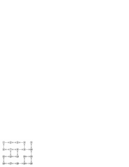
Watershed transform algorithm. We introduce an ordering function $\alpha:V\to\{1,2,...,|V|\}$ such that $\alpha(u)\neq\alpha(v)$ if and only if $u\neq v$ . We’ll refer to $\alpha(u)$ as the index of $u$ (Fig. 2(a)). In the first part of the algorithm we modify $D$ by removing edges. For all saddle vertices we keep only one outgoing edge - the one pointing to a vertex with the lowest index. In the next step we divide the non-minimal plateaus. We initialize a global FIFO queue $Q$ , mark all the plateau corner vertices as visited and insert them into $Q$ in increasing order of their index. While $Q$ is not empty we remove the vertex $v$ from the front of the queue, we then explore all the bidirectional edges $\{v,u\}$ . If $u$ is not visited, we mark it as such, insert it to the back of the queue and change the edge to be incoming $(v\leftarrow u)$ . Otherwise, if the vertex was already visited we just remove the edge. The resulting steepest descent graph is shown on Fig. 2(c) - the dotted edges are removed. Considering all the remaining edges as bidirectional, the connected components of the modified descent graph D will be the watershed basins of attraction.

The algorithm runs in linear time with respect to the number of edges in $G$ and produces an optimal partitioning as defined in [3]. The total number of segments in the partitioning will equal to the total number of regional minima. We defer the detailed algorithm listing, the proof of correctness and running time analysis to the supplementary material.

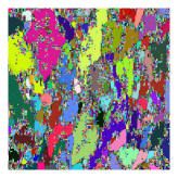
Reducing over-segmentation. Noisy values of disaffinities can produce severe over-segmentation (Fig. 3(c)). In order to reduce the over-segmentation we often merge adjacent segments with the saliency below some given threshold $T_{\min}$ [7]. The saliency of two adjacent segments is defined as the value of the minimal disaffinity between the vertices of the two segments. That means that we are confident that disaffinities below $T_{\min}$ connect vertices of the same segment. An equivalent segmentation can be obtained by replacing the weights of all edges in $G$ with the weight smaller than $T_{\min}$ to a common low value (e.g. $0$ ) before applying the watershed transform. We prove this claim in the supplementary material. To show confidence about high values of disaffinities, and in order to prevent undesired mergers, we introduce a threshold $T_{\max}$ by erasing all the edges from $G$ with the weight higher than $T_{\max}$ , and essentially setting them to $\infty$ . The $T_{\max}$ threshold can produce singleton vertices in $G$ . The singleton vertices are not assigned to any basin of attraction and are considered background, which is often a desired result.

3 Hierarchical Clustering of the Watershed Basin Graph

A hierarchical clustering of an undirected weighted graph treats each vertex as a singleton cluster and successively merges clusters connected by an edge in the graph. A cluster is always a connected subset of the graph’s vertices. Each merge operations creates a new level of the hierarchy - a flat segmentation where each cluster represents a segment. In single linkage clustering, each step merges two clusters connected by an edge with the lowest weight in the original graph. Single linkage clustering is equivalent to finding the minimum spanning tree of the graph [8].

In this section we propose a size-dependent single linkage clustering. The method can be applied to any edge weighted graph, however we find it superior when used on the watershed basin graph defined as follows. Let $V_{W}=\{B_{1},B_{2},\dots\}$ be the set of watershed basins obtained by the watershed transform of a graph $G=(V,E)$ . We define the watershed basin graph of $G$ as $G_{W}=(V_{W},E_{W})$ where an edge $\{B_{i},B_{j}\}$ exists in $E_{W}$ for all neighboring basins $B_{i}$ and $B_{j}$ , and has the weight $w(\{B_{i},B_{j}\})$ equal to the saliency of the two basins. We will refer to the vertices of the watershed basin graph as basins and to the edge weights as saliencies.

In our size-dependent single linkage clustering method, in each step we merge clusters with the lowest saliency that don’t satisfy a given predicate. Saliency of two clusters is defined as the minimal saliency of any two members:

d_{C_{1},C_{2}}=\underset{B_{i}\in C_{1},B_{j}\in C_{2},\{B_{i},B_{j}\}\in E_{W}}{\min}w(\{B_{i},B_{j}\})

(1)

At the last level of the hierarchy all pairs of clusters will satisfy the predicate.

Size-dependent comparison predicate. We define a predicate $\Lambda,$ for evaluating whether two clusters should be merged. The predicate is based on the sizes of the two clusters. Let $S(C)$ represent the size of $C$ (e.g. number of basins in the cluster or the sum of the basin sizes). We first define a non-increasing threshold function of a cluster size $\tau(s)$ . The value of $\tau(s)$ represents the maximal saliency allowed between a cluster of size $s$ and any adjacent cluster. Our predicate is then defined as:

\Lambda(C_{1},C_{2})=\begin{cases}\textrm{t{rue}}&\textrm{if }d_{C_{1},C_{2}}\geq\tau\left(\min\left\{S(C_{1}),S(C_{2})\right\}\right)\\ \textrm{false}&\textrm{otherwise{ }}\end{cases}

(2)

The intuition behind the predicate is to apply prior knowledge about the sizes of the true segments. With the threshold function we control the confidence required to grow a cluster of a certain size.

With a slight modification of the predicate we could allow for an arbitrary threshold function (changing the condition to $d_{C_{1},C_{2}}\geq\min\left\{\tau(S(C_{1})),\tau(S(C_{2}))\right\})$ . However, restricting the function to be non-decreasing allows us to design a more efficient algorithm. It is also more intuitive to allow higher saliency for merging small clusters and require lower saliency as the sizes of the clusters grow. As $\tau$ is required to be non-decreasing, we can find a non-increasing function $\omega$ such that when (2) is satisfied $\omega(d_{C_{1},C_{2}})\leq\min\left\{S(C_{1}),S(C_{2})\right\}$ is satisfied. This allows us to either specify either $\tau$ or $\omega$ used for the predicate. For example, when $\omega$ is constant the algorithm will tend to aggressively merge segments smaller than the given constant.

Algorithm 1 In our clustering algorithm we visit all the edges of the watershed basin graph in non-decreasing order and merge the corresponding clusters based on the introduced predicate.

1.

Order $E_{W}$ into $\pi(e_{1},\dots,e_{n})$ , by non-decreasing edge weight.
2.

Start with basins as singleton clusters $S^{0}=\{C_{1}=\{B_{1}\},C_{2}=\{B_{2}\},\dots\}$
3.

Repeat step $4$ for $k=1,\dots,n$
4.

Construct $S^{k}$ from $S^{k-1}$ . Let $e_{k}=\{B_{i},B_{j}\}$ be the $k$ -th edge in the ordering. Let $C_{i}^{k-1}$ and $C_{j}^{k-1}$ be components of $S^{k-1}$ containing $B_{i}$ and $B_{j}$ . If $C_{i}^{k-1}\neq C_{j}^{k-1}$ and $\Lambda(C_{i}^{k-1},C_{j}^{k-1})$ is not satisfied then $S^{k}$ is created from $S^{k-1}$ by merging $C_{i}^{k-1}$ and $C_{j}^{k-1}$ , otherwise $S^{k}=S^{k-1}.$
5.

Return the hierarchical segmentation $(S^{0},\dots,S^{n})$

Theorem 1 The highest level of the hierarchical segmentation produced by algorithm (1) will have the predicate $\Lambda$ satisfied for all pairs of the clusters. The complexity of the algorithm is $\left|E_{W}\right|\log\left|E_{W}\right|$ . The algorithm can be modified to consider only the edges of the minimum cost spanning tree of $G_{W}$ .

We defer the proof the supplementary material.

The steps 2-5 of the algorithm have near linear complexity. Once we have a sorted list of the edges we can re-run the algorithm for different threshold functions more efficiently.

(a)

(b)

(c)

(d)

(e)

(f)

(g)

(h)

Fig. 3.: Segmentation of a

256^{3}

EM image by our method and that of [5] (a) slice of the raw image; (b) slice of nearest neighbor disaffinity graph, with

xyz

disaffinities represented with RGB; (c) watershed transform of raw image; (d) watershed transform after preprocessing with

T_{\min}=0.01

and

T_{\max}=0.9

; (e) post-processing with size-dependent single linkage clustering using

\omega(w)=3000\left(1-w\right)

; (f, g) [5] with

k=0.5

yields severe oversegmentation while

k=10

merges neurons. (h) ground truth segmentation from human expert

4 Results

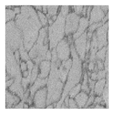
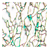
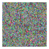
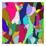
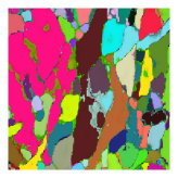
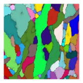
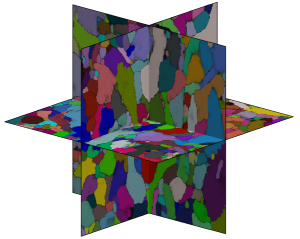
We applied our method to 3D electron microscopic brain images [9] (Fig. 3(a)). Disaffinity graphs were computed using convolutional networks [10] (Fig. 3(b)). The watershed transform produced severe oversegmentation (Fig. 3(c)), which was reduced by pre-processing the disaffinity graph with upper and lower thresholds (Fig. 3(d)). Size-dependent single linkage clustering further reduced oversegmentation (Fig. 3(e)). The first function enforced all the segments to be at least some minimal size. The second and the third functions require the minimal size of the segment to be proportional to the affinity (or the square of affinity).

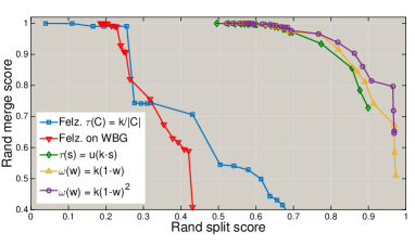
Measuring the quality of the segmentations. We evaluated the segmentations by comparing to the ground truth generated by a human expert. Split and merge scores were computed by

V_{\textrm{split}}=\frac{{\sum_{ij}p_{ij}^{2}}}{\sum_{k}t_{k}^{2}}\textrm{ and }V_{\textrm{merge}}=\frac{{\sum_{ij}p_{ij}^{2}}}{\sum_{k}s_{k}^{2}}

(3)

where $p_{ij}$ is the probability that a randomly chosen voxel belongs to segment $i$ in the proposed segmentation and segment $j$ in the ground truth, $s_{i}$ and $t_{j}$ are probabilities of a randomly chosen voxel belonging to predicted segment $i$ and ground truth segment $j$ respectively. The scores are similar to the Rand index, a well-known metric for clustering [11], except that they distinguish between split and merge errors. Higher scores mean fewer errors. Scoring was restricted to the foreground voxels in the ground truth. We tested our method with several threshold functions, and also applied the method of [5] to the disaffinity graph and to the watershed basin graph. Our method achieved superior scores (Fig. 4(a)). The paremeter $k$ in both methods determines the trade-off between the amount of mergers and splits. When $k$ in the method of [5] is optimized to have approximately the same amount of mergers as our method, large amount of splits are introduced (Fig. 3(f)) and vice versa (Fig. 3(g)).

In conclusion, the runtime of our method makes it very suitable for segmenting very large images. It greatly outperforms other methods similar in runtime complexity. Our method can greatly reduce the oversegmentation while introducing virtually no mergers.

References

1.

Tomer, R., Khairy, K., Amat, F., Keller, P.J.: Quantitative high-speed imaging of entire developing embryos with simultaneous multiview lightsheet microscopy. Nature Methods 9 755–763 (2012)
2.

Marx, V.: Neurobiology: Brain mapping in high resolution. Nature 503 147–52 (2013)
3.

Cousty, J., Bertrand, G., Najman, L., Couprie, M.: Watershed cuts: Minimum spanning forests and the drop of water principle. IEEE Transactions on Pattern Analysis and Machine Intelligence 31 1362–1374 (2009)
4.

Felzenszwalb, P.F., Huttenlocher, D.P.: Efficient graph-based image segmentation. International Journal of Computer Vision 59 167–181 (2004)
5.

Guimarães, S.J.F., Cousty, J., Kenmochi, Y., Najman, L.: A Hierarchical Image Segmentation Algorithm Based on an Observation Scale. 116– 125 (2012)
6.

Cousty, J., Bertrand, G., Najman, L., Couprie, M.: Watershed cuts: Thinnings, shortest path forests, and topological watersheds. IEEE Transactions on Pattern Analysis and Machine Intelligence 32 925–939 (2010)
7.

Najman, L., Schmitt, M.: Geodesic Saliency of Watershed Contours and Hierarchical Segmentation. Analysis 18 1163–1173 (1996)
8.

Gower, J.C., Ross, G.J.S.: Minimum Spanning Trees and Single Linkage Cluster Analysis. Journal of the Royal Statistical Society. Series C (Applied Statistics) 18 54–64 (1969)
9.

Briggman, K.L., Helmstaedter, M., Denk, W.: Wiring specificity in the direction-selectivity circuit of the retina. Nature 471 183–188 (2011)
10.

Helmstaedter, M., Briggman, K.L., Turaga, S.C., Jain, V., Seung, H.S., Denk, W.: Connectomic reconstruction of the inner plexiform layer in the mouse retina. Nature 500 168–74 (2013)
11.

Rand, W.M..: Objective Criteria for the Evaluation of Clustering Methods. Journal of the American Statistical Association 66 846–850 (1971)