Heavy tails in the distribution of time-to-solution for classical and quantum annealing
Abstract
For many optimization algorithms the time-to-solution depends not only on the problem size but also on the specific problem instance and may vary by many orders of magnitude. It is then necessary to investigate the full distribution and especially its tail. Here we analyze the distributions of annealing times for simulated annealing and simulated quantum annealing (by path integral quantum Monte Carlo) for random Ising spin glass instances. We find power-law distributions with very heavy tails, corresponding to extremely hard instances, but far broader distributions – and thus worse performance for hard instances – for simulated quantum annealing than for simulated annealing. Fast, non-adiabatic, annealing schedules can improve the performance of simulated quantum annealing for very hard instances by many orders of magnitude.
Non-convex optimization problems arise in a wide range of areas, from industrial applications to scientific research. Many challenging optimization problems belong to the class of non-deterministic polynomial-time hard (NP-hard) problems. For these problems, which includes the famous traveling salesman problem, no efficient algorithm is known that scales polynomially with problem size. In the absence of efficient exact solvers, often heuristic algorithms are the best choice. For many algorithms, and especially probabilistic annealing strategies Kirkpatrick et al. (1983); Suman and Kumar (2006); Kadowaki and Nishimori (1998); Santoro et al. (2002); Santoro and Tosatti (2006), the time to find a (near)-optimal solution may depend not just on the problem size , but may vary greatly – by many orders of magnitude – from instance to instance. In such cases one usually quotes the typical performance given by the median time-to-solution.
Despite its common use, the median time-to-solution is often not the quantity that dictates efficiency, since one generally wants to solve more than half of the problem instances. In particular, in the case of broad distributions of the time-to-solutions, higher quantiles (such as the 99-th percentile) may be better indicators of the performance of an optimization algorithm. In this Letter we demonstrate that when analyzing the performance of optimization algorithms, it is very important to consider the tails of the time-to-solution distribution and not only averages or median performances.
As a specific example we consider the problem of finding the ground states of Ising spin glasses on chimera graphs. In these models Ising spins that can take values should be chosen to minimize the total energy,
| (1) |
where the coupling constants take random values on the edges of the so-called Chimera graph. For more information see the Supplementary Material. This quasi-two-dimensional graph with eight spins per unit cell is non-planar, which makes the problem of finding the ground state of the Ising spin glass NP-hard Barahona (1982).
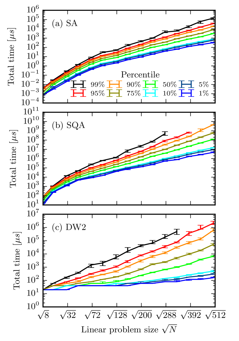
The Ising spin glass problem on the chimera graph has recently received special attention, since this graph is implemented in the optimization devices built by the Canadian company D-Wave systems Johnson et al. (2011), whose performance has been controversially discussed in the recent literature Boixo et al. (2014); Rønnow et al. (2014); Shin et al. (2014); McGeoch and Wang (2013); Dash (2013); Katzgraber et al. (2014). We summarize, in Fig. 1 previous results Rønnow et al. (2014) of the scaling of the time-to-solution (TTS) as a function of problem size for three different approaches: a simulated annealer (SA), a simulated quantum annealer (SQA) using path integral quantum Monte Carlo, and a D-Wave Two device (DW2). Note one striking feature of these results: there is a huge spread in TTS between easy and hard instances (the 99th percentile), which varies by three orders of magnitude for SA, and by even more for SQA and DW2. The hard instances completely dominate the TTS. Below we will quantitatively analyze the distribution of TTS for the hardest instances, and show how it can be substantially reduced for SQA by using non-adiabatic annealing schedules.
Simulated annealing (SA) is inspired by annealing, a process in metallurgy by which a material is heated up and then slowly cooled down in order to relieve internal stresses. In 1983, Kirkpatrick and coworkers Kirkpatrick et al. (1983) showed that simulating an annealing process a Monte Carlo simulation can be used as a general purpose heuristic solver for optimization problems, which is widely used in many application areas Suman and Kumar (2006). By slowly decreasing the temperature the system can relax into a low-energy state, escaping local minima by thermal activation over barriers. Implementation details are discussed in the Supplementary Material.
Inspired by the phenomenon of quantum tunneling, quantum annealing (QA) uses quantum fluctuations instead of thermal fluctuations to explore the configuration space Ray et al. (1989); Finnila et al. (1994); Kadowaki and Nishimori (1998); Farhi et al. (2001); Das and Chakrabarti (2008). It employs a time-dependent Hamiltonian,
| (2) |
where is a driver Hamiltonian implementing quantum dynamics, and the problem Hamiltonian implements the Ising spin glass Eq. (1) using quantum spin-1/2 particles. and are Pauli matrices. At the beginning of the annealing schedule when and we start with only . The spins are initialized in the ground state aligning along the x-axis. During the annealing process we decrease and increase , so that at the end of the annealing at time , we end up with the Ising spin glass of Eq. (1). The Hamiltonian is changed slowly enough such that the system stays in (or close to) the ground state at all times. This process takes place at a constant finite temperature and therefore constant inverse temperature , where is the Boltzmann constant. The D-Wave devices have been designed to implement quantum annealing using superconducting flux qubits Johnson et al. (2011) in a physical device.
Quantum annealing can also be implemented as simulated quantum annealing (SQA) on a classical computer using a path integral quantum Monte Carlo simulation Santoro et al. (2002); Santoro and Tosatti (2006); Heim et al. (2015). Furthermore, by replacing the quantum spins in Eq. (2) with two-dimensional classical rotor magnets a mean-field version (MFA) Shin et al. (2014) can be obtained as a semi-classical version of SQA Albash et al. (2014). Details of the SQA and MFA algorithms and their implementations are presented in the Supplementary Material. Note that annealing times for SA, SQA and MFA are measured in numbers of sweeps, where one sweep is defined as one attempted update for each spin.
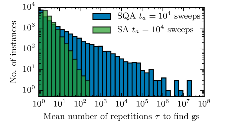
For each problem size we created 20000 different random problem instances with couplings . For each instance, after determining the exact ground state energy using an exhaustive search algorithm we repeatedly performed SA, SQA and MFA simulations until we found a ground state at least 100 times for each algorithm. For SQA with spins and annealing time sweeps we never found the ground state of the hardest instances despite billions of attempts. We thus focus on the case of spins for our quantitative analysis, where all algorithms found the ground states of all problem instances with reasonable effort. From the number of repetitions required to find the ground state one hundred times we then calculated the single-run success probability and the mean number of repetitions required to find the ground state.
Plotting histograms of for 20000 instances with we arrive at the distributions shown in Fig. 2. We see very slowly decaying power-law tails, consistent with the wide spread of quantiles in Fig. 1. We also see that while the median times are very similar ( for SA and for SQA), there is a substantial quantitative difference between the distributions. For SA tails extend up to large values of , but for SQA to values of which is more than 5 orders of magnitude larger. The median times are thus neither indicative of the time needed to solve hard problem instances, nor of the relative performance of the two algorithms!
To analyze this significant difference in the tail distribution function in detail, we use extreme value theory (EVT) to obtain a good estimate for the tail distribution of given only a limited data set and specifically to calculate the so-called shape parameter , which gives information about its power-law tail. Let us denote by the unknown distribution function of a random variable , e.g. the distribution of for a specific algorithm. If satisfies certain conditions (described in the Supplementary Material) then the Balkema-de Haan-Pickands (BdHP) theorem Balkema and de Haan (1974); Pickands III (1975) states that the tail of the distribution function, for larger than a high threshold , is approximated by a generalized Pareto (GP) distribution function , i.e.
| (3) |
The GP distribution function with threshold/location parameter , shape parameter , scale parameter is given by
| (4) |
which is defined on Reiss and Thomas (2007); Falk et al. (2011); Coles (2001). For one takes the limit ,
| (5) |
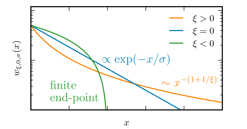
The qualitative behavior of the GP distribution function is given by its shape parameter , which turns out to be very useful when benchmarking different algorithms. The shape parameter is independent of the threshold and of any linear transformations on , e.g. considering the number of spin flips to find the ground state instead of . The probability density has three distinct tail behaviors, shown in Fig. 3, depending on the sign of . It is bounded for , exponentially decaying for and slowly decaying as a power-law for , which we also refer to as having a heavy tail. Note that the -th moment of diverges for McNeil et al. (2005).
If a heuristic algorithm has , then hard instances dominate the average time-to-solution. If the shape parameter the average run-time of an instance is infinite. In our case of discrete couplings , there is only a finite set of instances for each . The conditions of the the BdHP theorem are thus not satisfied because the distribution of is discrete with only a finite number of points in its support (Arnold et al., 2008, p. 217). Nevertheless we can still use the GP distribution to analyze our data, and obtain excellent fits (see Supplementary Material). The main consequence of a finite set of instances is that differs from the GP distribution function for the hardest instances, and thus for example the mean is not infinite but dominated by the hardest instances. In the Supplementary Material we show that the mean is not converging for using 20000 problem instances.
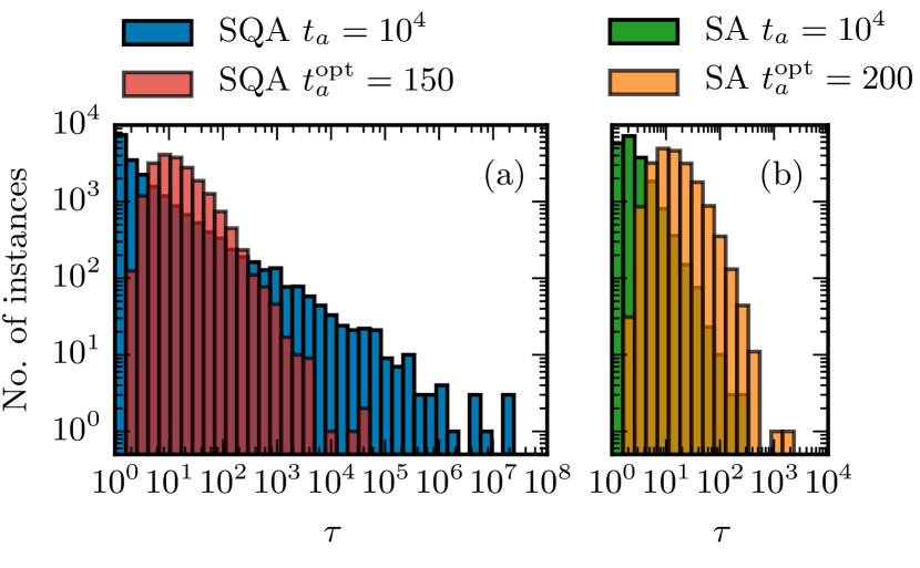
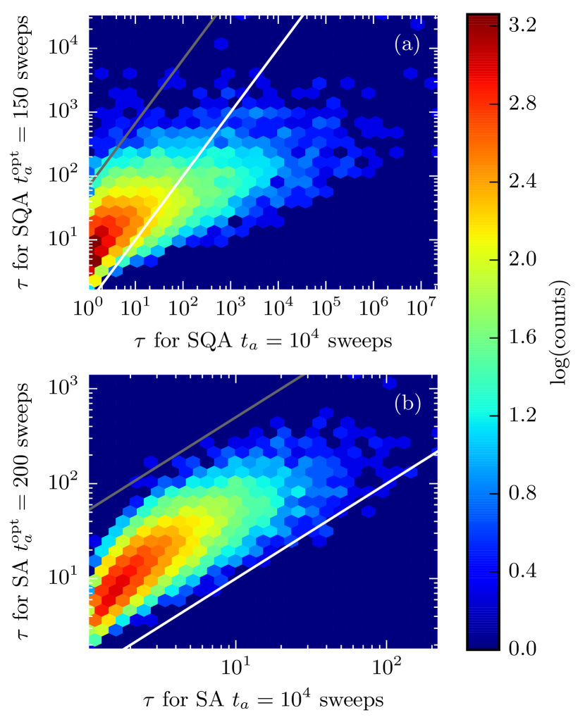
We start, by investigating the effects of annealing time on the distribution. In Fig. 4 we compare the distributions for sweeps (which for SQA with was found to give good correlations with a D-Wave One device Boixo et al. (2014)) to simulations run with the (size-dependent) optimal that minimizes the total effort (see Ref. Rønnow et al., 2014 and the Supplementary Material). The surprising result is that performing SQA with a fast schedule of only sweeps leads to a more compact distribution with much faster decaying tails. While easy instances may need a few more repetitions, hard instances need far less repetitions to find the ground state.
As the correlation plot in Fig. 5 shows, the relative hardness of an instance doesn’t change significantly when changing , but the single-run success probability of SQA increases for more than 10% of the instances when SQA is run faster. This is opposite to SA where for almost all instances decreases when annealing faster. In both cases, however, the total effort decreases for almost all instances. Even though more repetitions are needed, this is more than compensated by the faster annealing time. For SQA, the combined effect of needing 688 times fewer repetitions and performing only 150 instead of sweeps per repetition reduces the total effort for the hardest of our instances by a factor 45866!
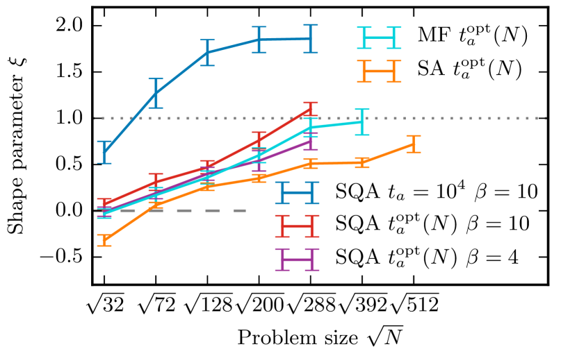
To quantify the difference in the tail distribution functions we fit them to GP distribution functions and plot the size-dependence of the shape parameter for SA, SQA and MFA in Fig. 6. For SQA we use the two schedules discussed above and additionally a third schedule, with sweeps but a higher temperature , which is the optimal temperature for MFA (see Supplementary Material). All algorithms have heavy tails, , for problems with size , and is increasing with system size. For SQA using and we find already for , indicating that the mean time-to-solution is already divergent and dominated by the hardest instances. As we already saw above for , the tail behavior of SQA improves when using faster annealing schedules, and further small improvements are obtained by raising the temperature. While SQA with the best setting and MFA have the same , SA has smaller , indicating a faster decaying tail and better performance on hard instances.
Our results show that the tail behavior is the important measure of performance when considering the performance of an optimization algorithm since the hardness of an instance is a priori unknown. Therefore one has to choose a large enough run-time such that a high percentile of random instances are solved. Considering just the typical (median) performance of an optimization algorithm can be misleading in the presence of broad heavy-tailed distributions. The median effort misses the important fact that already at moderate problem sizes the mean time-to-solution can diverge, indicating that the hardest instances dominate the average. As one typically wants to solve much more than half of the problem instances, reducing the tails of the distribution is crucial to optimize the performance of an optimization algorithm.
One surprising result we obtained here is that for simulated quantum annealing, fast non-adiabatic schedules show far superior performance than slow adiabatic annealing schedules that would naïvely seem superior. This observation is consistent with results obtained in Refs. Heim et al. (2015); Crosson et al. (2014) which showed that for some instances fast annealing schedules can help a (simulated) quantum annealer escape local minima. As good agreement was found between SQA and the D-Wave devices, we expect that similarly faster annealing schedules can help the performance not only of simulated quantum annealers but also of physical quantum annealing devices.
The tail behavior is also important for extrapolating the performance of annealers to larger sizes. The tails are indicative of harder problems that will dominate for larger problem sizes. We thus expect scaling differences between different annealers to first show up in the tails.
We acknowledge discussions with Sergio Boixo, Paul Embrechts, Hartmut Neven and Diethelm Würtz and thank Ethan Brown for proofreading and Coal Ila for inspiration. This work has been supported by the Swiss National Science Foundation through the National Competence Center in Research QSIT and is based upon work supported in part by IARPA via MIT Lincoln Laboratory Air Force Contract No. FA8721-05-C-0002.
References
- Kirkpatrick et al. (1983) S. Kirkpatrick, C. D. Gelatt, and M. P. Vecchi, Science 220, 671 (1983).
- Suman and Kumar (2006) B. Suman and P. Kumar, J. Oper. Res. Soc. 57, 1143 (2006).
- Kadowaki and Nishimori (1998) T. Kadowaki and H. Nishimori, Physical Review E 58, 5355 (1998).
- Santoro et al. (2002) G. E. Santoro, R. Martonak, E. Tosatti, and R. Car, Science 295, 2427 (2002).
- Santoro and Tosatti (2006) G. E. Santoro and E. Tosatti, J. Phys. A: Math. Gen. 39, R392 (2006).
- Rønnow et al. (2014) T. F. Rønnow, Z. Wang, J. Job, S. Boixo, S. V. Isakov, D. Wecker, J. M. Martinis, D. A. Lidar, and M. Troyer, Science 345, 420 (2014).
- Barahona (1982) F. Barahona, J. Phys. A: Math. Gen. 15, 3241 (1982).
- Johnson et al. (2011) M. W. Johnson, M. H. S. Amin, S. Gildert, T. Lanting, F. Hamze, N. Dickson, R. Harris, A. J. Berkley, J. Johansson, P. Bunyk, E. M. Chapple, C. Enderud, J. P. Hilton, K. Karimi, E. Ladizinsky, N. Ladizinsky, T. Oh, I. Perminov, C. Rich, M. C. Thom, E. Tolkacheva, C. J. S. Truncik, S. Uchaikin, J. Wang, B. Wilson, and G. Rose, Nature 473, 194 (2011).
- Boixo et al. (2014) S. Boixo, T. F. Rønnow, S. V. Isakov, Z. Wang, D. Wecker, D. A. Lidar, J. M. Martinis, and M. Troyer, Nat. Phys. 10, 218 (2014).
- Shin et al. (2014) S. W. Shin, G. Smith, J. A. Smolin, and U. Vazirani, (2014), arXiv:1401.7087v2 [quant-ph] .
- McGeoch and Wang (2013) C. C. McGeoch and C. Wang, in Proceedings of the 2013 ACM Conference on Computing Frontiers (2013).
- Dash (2013) S. Dash, (2013), arXiv:1306.1202v2 [math] .
- Katzgraber et al. (2014) H. G. Katzgraber, F. Hamze, and R. S. Andrist, Physical Review X 4, 021008 (2014).
- Ray et al. (1989) P. Ray, B. K. Chakrabarti, and A. Chakrabarti, Physical Review B 39, 11828 (1989).
- Finnila et al. (1994) A. B. Finnila, M. A. Gomez, C. Sebenik, C. Stenson, and J. D. Doll, Chemical Physics Letters 219, 343 (1994).
- Farhi et al. (2001) E. Farhi, J. Goldstone, S. Gutmann, J. Lapan, A. Lundgren, and D. Preda, Science 292, 472 (2001).
- Das and Chakrabarti (2008) A. Das and B. K. Chakrabarti, Rev. Mod. Phys. 80, 1061 (2008).
- Heim et al. (2015) B. Heim, T. F. Rønnow, S. V. Isakov, and M. Troyer, Science (2015), arXiv:1411.5693 .
- Albash et al. (2014) T. Albash, T. Rønnow, M. Troyer, and D. Lidar, (2014), arXiv:1409.3827 [quant-ph] .
- Balkema and de Haan (1974) A. A. Balkema and L. de Haan, Ann. Probab. 2, 792 (1974).
- Pickands III (1975) J. Pickands III, Ann. Stat. 3, 119 (1975).
- Reiss and Thomas (2007) R.-D. Reiss and M. Thomas, Statistical Analysis of Extreme Values: with Applications to Insurance, Finance, Hydrology and Other Fields, 3rd ed. (Birkhäuser, 2007).
- Falk et al. (2011) M. Falk, J. Hüsler, and R.-D. Reiss, Laws of Small Numbers: Extremes and Rare Events, third, revised and extended edition ed. (Birkhäuser, 2011).
- Coles (2001) S. Coles, An Introduction to Statistical Modeling of Extreme Values, Springer Series in Statistics (Springer, 2001).
- McNeil et al. (2005) A. J. McNeil, R. Frey, and P. Embrechts, Quantitative Risk Management: Concepts, Techniques, and Tools (Princeton University Press, 2005).
- Arnold et al. (2008) B. C. Arnold, N. Balakrishnan, and H. N. Nagaraja, A First Course in Order Statistics (Society for Industrial and Applied Mathematics, 2008).
- Crosson et al. (2014) E. Crosson, E. Farhi, C. Lin, H. H. Lin, and P. Shor, (2014), arXiv:1401.7320 .
- Metropolis et al. (1953) N. Metropolis, A. W. Rosenbluth, M. N. Rosenbluth, A. H. Teller, and E. Teller, J. Chem. Phys. 21, 1087 (1953).
- Isakov et al. (2014) S. V. Isakov, I. N. Zintchenko, T. F. Rønnow, and M. Troyer, (2014), arXiv:1401.1084v2 [cond-mat.dis-nn] .
- Suzuki (1976) M. Suzuki, Prog. Theor. Phys. 56, 1454 (1976).
- Pierre et al. (1987) L. Pierre, T. Giamarchi, and H. Schulz, Journal of Statistical Physics 48, 135 (1987).
- de Haan (1990) L. de Haan, Statistica Neerlandica 44, 45 (1990).
- Dietrich et al. (2002) D. Dietrich, L. de Haan, and J. Hüsler, Extremes 5, 71 (2002).
- Hüsler and Li (2006) J. Hüsler and D. Li, Extremes 9, 69 (2006).
- Drees (2012) H. Drees, AStA Advances in Statistical Analysis 96, 225 (2012).
- Castillo et al. (2004) E. Castillo, A. S. Hadi, N. Balakrishnan, and J. M. Sarabia, Extreme Value and Related Models with Applications in Engineering and Science (Wiley-Interscience, 2004).
- Original S functions written by Janet E. Heffernan with R port and R documentation provided by Alec G. Stephenson. (2012) Original S functions written by Janet E. Heffernan with R port and R documentation provided by Alec G. Stephenson., ismev: An Introduction to Statistical Modeling of Extreme Values. (2012), r package version 1.39.
- Pfaff and McNeil (2012) B. Pfaff and A. McNeil, evir: Extreme Values in R. (2012), r package version 1.7-3.
Supplementary Material for “Heavy tails in the distribution of time-to-solution for classical and quantum annealing”
I Annealing algorithms
In the following we present implementation details for the three annealing algorithms.
I.1 Simulated annealing
SA is a Monte Carlo algorithm which generates states of a classical system in thermal equilibrium whose energy is described by the following Hamiltonian
| (6) |
Our SA code generates new states by flipping a single spin and accepting the spin flip according to the Metropolis update rule Metropolis et al. (1953). Hence, the probability to generate a state with energy is proportional to the Boltzmann weight , where is the inverse temperature. Over the annealing time , which is measured in numbers of sweeps (one sweep is an attempted flip of every spin in the system), the temperature is slowly decreased. In the beginning, when the temperature is high, SA has a large probability to generate high energy states, called thermal excitations, which allow SA to escape from a local minimum. In the end, the temperature is low such that mostly states with lower energy are accepted and the system relaxes into the local minimum. For these instances with , we linearly increase the inverse temperature over the annealing time . In order to reduce CPU time, our implementation uses forward computation of the energies as described in Ref. Isakov et al. (2014).
I.2 Simulated quantum annealing
SQA is a Monte Carlo algorithm which generates states of a quantum system in thermal equilibrium. During the annealing the temperature is kept constant. The Hamiltonian of the system is time dependent and given by Eq. (2) in the main paper. At the beginning of the annealing schedule when and we start with only . We use a linear schedule, i.e. we linearly decrease and increase , so that at the end of the annealing at time , the Hamiltonian of the system is given by .
SQA uses the Suzuki-Trotter formalism with which a -dimensional Ising model with a transverse field is mapped
to a ()-dimensional Ising model at finite temperature Suzuki (1976). Here we use a discrete-time path integral formulation with 32 imaginary time slices and we
build clusters along the imaginary time direction. On a technical level, we exploit a random bit algorithm explained in Ref. Pierre et al. (1987)
to form new domain walls in all 32 Trotter slices simultaneously.
We analyze SQA as simulation of a physical system, which means that in the end of annealing, the success probability of finding the ground state is given by the number of Trotter slices which reached the ground state divided by 32 (the total number of Trotter slices). This means for example that if half the Trotter slices are in the ground state, we count this run as having found the ground state only with probability 0.5, because an actual quantum system would collapse into one of the Trotter slices. One could on contrary also analyze SQA as a purely classical algorithm and define that a single run has found the ground state energy with probability 1 if at least one Trotter slices is in the ground state, as one can check all Trotter slices in a classical code. This way of analyzing SQA resulted in very similar shape parameters of the fitted GP distribution functions for , which means there is no qualitative difference in the tail behavior and therefore we only show the results of analyzing SQA as a simulation of a physical system throughout the whole paper.
I.3 Mean-field quantum annealing
MFA is a mean-field version of simulated quantum annealing. A spin is represented by a classical magnet pointing in some direction in the XZ plane Shin et al. (2014). The classical time-dependent Hamiltonian is then given by:
| (7) |
MFA is a Monte Carlo algorithm which generates states of this system at thermal equilibrium and the temperature is again kept constant. A new state is generated by proposing an update of spin by choosing uniform randomly a new angle and then accepting or rejecting this update according to the Metropolis update rule Metropolis et al. (1953). We use the same linear schedule for the constants and as in the case for SQA and all spins are initialized to be aligned in x-direction at . Our MFA implementation follows the description in Ref. Shin et al. (2014), but differs by using 1024 element lookup tables with precomputed values of and .
II Problem instances
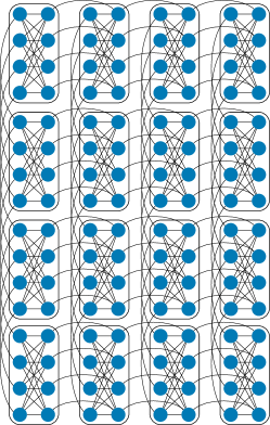
The present analysis was carried out on Ising spin glasses with Chimera topology. The Chimera graph is formed by a two-dimensional lattice built from eight-spin unit cells that each form a complete bipartite graph . Fig. 7 shows the chimera graph for 128 spins, corresponding to unit cells. We used graphs with unit cells and spins, with ranging from 2 to 8. The couplings between the spins were randomly chosen to be .
To find the ground states of these Ising spin glasses, we implemented an exact solver using dynamic programming. The solver exploits the limited tree-width of the Chimera graph which allows one to perform an exhaustive search up to 512 spins.
Note that since Chimera graphs are bipartite, all our Monte Carlo annealing algorithms could potentially be parallelized efficiently because spins in one sublattice couple only to spins in the other sublattice and hence all spins in one sublattice can be updated simultaneously.
III Optimal number of sweeps
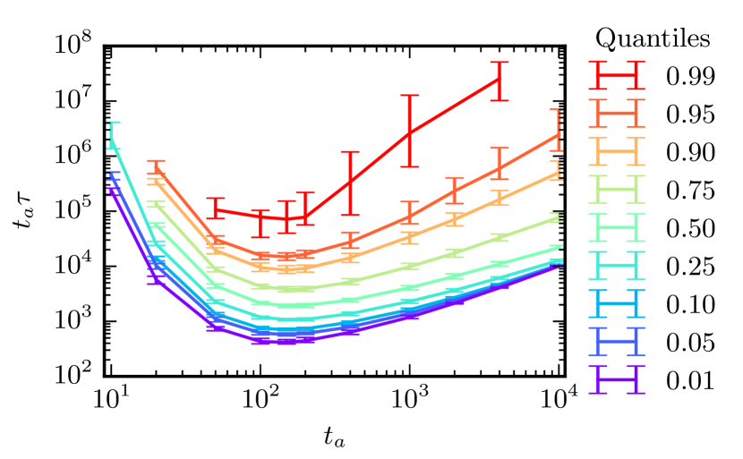
When investigating the scaling of annealers with problem size one has to carefully choose optimal parameters or one might draw wrong conclusions Boixo et al. (2014); Rønnow et al. (2014). One could, for instance, choose to run the annealer times and each time anneal for time and then choose the lowest lying state found, or, as an extreme case example, one could choose to make a single annealing run over a time span . The result in the two cases are very different, even though the total annealing time is equal in both cases.
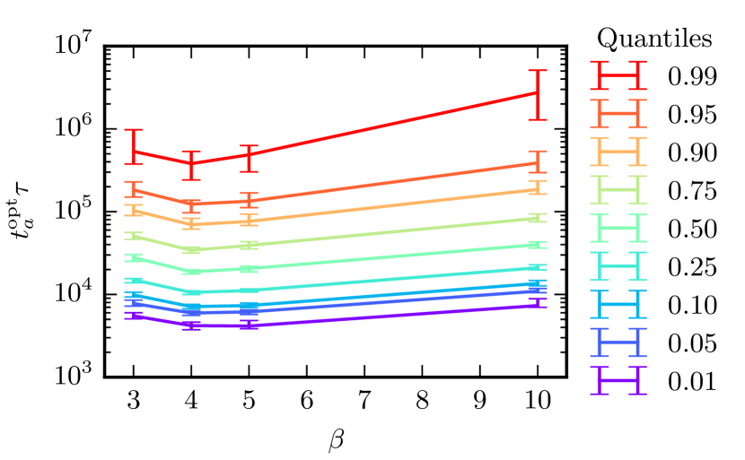
To make extrapolations to asymptotic scaling one needs to use an optimal annealing time , which is defined to be the number of sweeps which minimizes the total effort , where is the mean number of repetitions required to find the ground state. See Fig. 8. Note that the minima for the different quantiles are usually at roughly the same and the minima are quite broad and flat. Thus does not have to be determined with very high accuracy. The optimal annealing times are listed in Tab. 1 for SA, SQA and MFA.
| of SA | of SQA | of MFA | ||||||
|---|---|---|---|---|---|---|---|---|
| 32 | 10 | 20 | 20 | 20 | 50 | |||
| 72 | 25 | 50 | 50 | 100 | 100 | |||
| 128 | 70 | 100 | 100 | 500 | 200 | |||
| 200 | 200 | 150 | 150 | 2000 | 1000 | |||
| 288 | 300 | 200 | 400 | 5000 | 2000 | |||
| 392 | 650 | 400 | 1000 | 5000 | ||||
| 512 | 1500 | 400 | 1000 | 5000 | ||||
IV Optimal temperature of MFA
For the MFA algorithm we determined that the optimal inverse temperature is which minimizes the total effort required to find the ground state, , for most quantiles and problem sizes . See Fig. 9 which shows the case for .
V Extreme Value Theory
In this section we summarize the important parts of Extreme Value Theory (EVT) which are used in the main paper. A detailed discussion can be found in the cited papers and textbooks. Here we will state the Balkema-de Haan-Pickands (BdHP) theorem, which says that if satisfies the extreme value condition, then for . We will then discuss why our doesn’t satisfy the extreme value condition, but show that nevertheless our empirical data indicates that for is a good model for the range of which we are interested.
V.1 Theory
Let be a random variable, i.e. the run-time of an instance using a specific algorithm, which is described by the unknown distribution function .
Then the exceedance distribution function over a threshold , , is defined as
| (8) |
The Balkema-de Haan-Pickands theoremBalkema and de Haan (1974); Pickands III (1975) now says that if has, for some choice of constants and , a continuous limiting distribution function as goes to the right endpoint of F, which is also called the extreme value condition Reiss and Thomas (2007), then:
with threshold/location parameter , shape parameter , scale parameter and is a generalized Pareto (GP) distribution function
| (9) |
which is defined on Reiss and Thomas (2007); Falk et al. (2011); Coles (2001). For one has to take the limit :
| (10) |
For a large enough threshold this theorem provides a parametric model for the exceedance distribution function . The parameters and can be estimated by fitting the exceedances to as explained later. If is a good approximation, then it follows from the definition of that Reiss and Thomas (2007)
| (11) |
| (12) |
| (13) |
The shape parameters of the GP distribution function which approximates or are identical. And in contrast to the scale parameter which is dependent on the chosen threshold , the shape parameter is independent of , i.e. suppose that the threshold is high enough such that then if exceedances over a higher threshold are fitted, it results in the same shape parameter because of the peak-over-threshold stability of GP distribution functions : with Reiss and Thomas (2007).
In practice GP distribution functions are used as the canonical distribution function for modeling exceedances over a high threshold, see for example McNeil et al. (2005).
Moreover, as the distribution function of interest is unknown, it is commonly assumed as a null-hypothesis that satisfies the extreme value condition and hence it can be approximated by a GP distribution function above a high threshold. Tests on the data and fitted model should be performed to potentially reject the null-hypothesis, which we introduce in the next subsection.
The estimated GP distribution functions are often used to make predictions of rare events, which are even more extreme than what has already been observed and used for the fitting of the GP distribution parameters. For example, extreme value analysis is used to plan the heights of sea dikes in the Netherlands such they fail no more than once in 10’000 years on average, but the data for the model fitting consists of the sea level from the last 100 years only de Haan (1990).
In our case the extreme value condition is not satisfied, because as already stated in the main paper, our distribution functions of are discrete with only a finite number of points in its support, and therefore the extreme value condition doesn’t hold, see (Arnold et al., 2008, p.217). Nevertheless we assume as a null-hypothesis that in the range of above the threshold which we are interested. We are not interested in the very largest , e.g. the hardest 0.999999 quantile of our instances, because our problem of finding the ground state energy is NP hard, so the hardest instances are commonly assumed to be out of reach for current algorithms. In the next subsection we will see that the null-hypothesis cannot be rejected for our range of data and that the obtained GP distribution functions show excellent model fits, which justifies the use of GP distribution functions to fit our data.
V.2 Fitting Procedure
Here we introduce tests which could reject the null-hypothesis that our unknown distribution function satisfies the extreme value condition and show how to choose a high enough threshold .
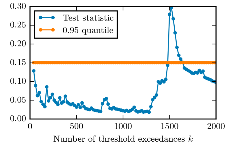
A common statistical approach to check the null-hypothesis is to estimate the parameters of the GP distribution function from the exceedances over a threshold of the data. Based on these estimators, tail probabilities and quantiles are deduced. Then graphical methods are used to analyze the goodness-of-fit using for example QQ and PP plots (Reiss and Thomas, 2007, p.145). These graphical methods are introduced in the next subsection and the results didn’t reject the null-hypothesis. In addition we used a method presented in Dietrich et al. (2002) to test the null-hypothesis, that satisfies the extreme value condition with some additional (second order) condition. A review is given in (Reiss and Thomas, 2007, p.144-151) and in the paper by Hüsler and Li Hüsler and Li (2006), where they also provide a R program code. This code is used in our paper to calculate the test statistics and the 0.95 quantiles of the limiting random variables by moment estimation for different number of threshold exceedances, an example is shown in Fig. 10. The test statistic depends on the chosen threshold value. We saw that if the threshold value was too low, this test rejects the null-hypothesis, which provides us a hint on the smallest possible threshold value. For all the chosen thresholds in this paper this test method doesn’t reject the null-hypothesis.
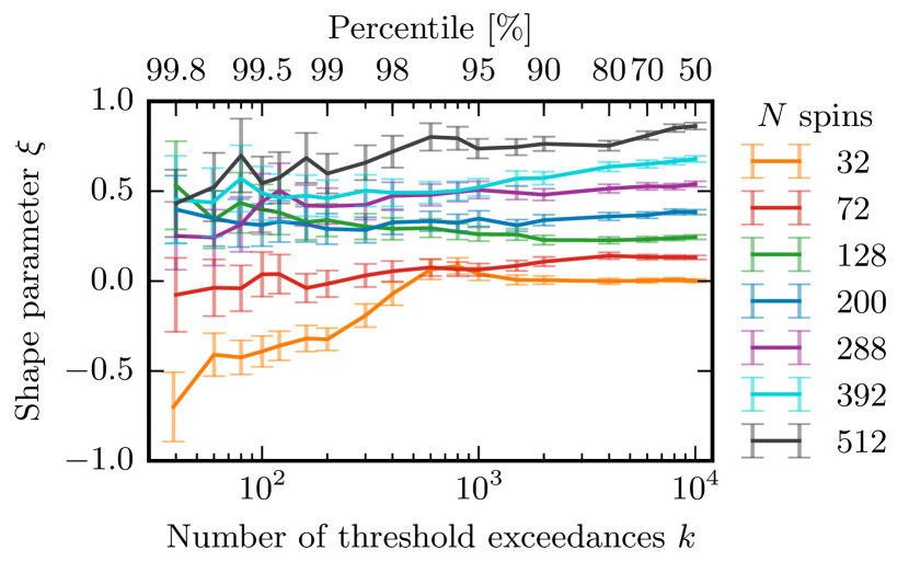
There are automatic ways of choosing a high enough threshold (Reiss and Thomas, 2007, p.137), however, we used two manual method which might achieve better fitting results: First a range of thresholds is chosen and the exceedances over these thresholds are used to estimate the parameters of the GP distribution functions by the Maximum Likelihood Estimation (MLE) method Coles (2001); Castillo et al. (2004). We used MLE implementations for extreme value theory from the two libraries ismev and evir Original S functions written by Janet E. Heffernan with R port and R documentation provided by Alec G. Stephenson. (2012); Pfaff and McNeil (2012) and 20’000 random problems are used for every algorithm, schedule and system size. The estimated shape parameter as a function of the threshold is plotted in Fig. 11. Because of the peak-over-threshold stability of the GP distribution function, the estimated shape parameter should be constant for thresholds if the threshold is already high enough. Therefore, there are usually three regions in Fig. 11: For a very high threshold there are only a few exceedances and hence the shape parameter fluctuates strongly. For a high threshold the shape parameter is stable around the true value. For a too low threshold there are too many exceedances and the extreme value condition might not be satisfied, this can be detected if the shape parameter is not constant or by testing the null-hypothesis, see Fig. 10. Now we have a range of threshold which seem to be high enough. To choose the exact threshold we used the PP and QQ plots to check which threshold shows the best model fit.
Evaluation of Model Fit
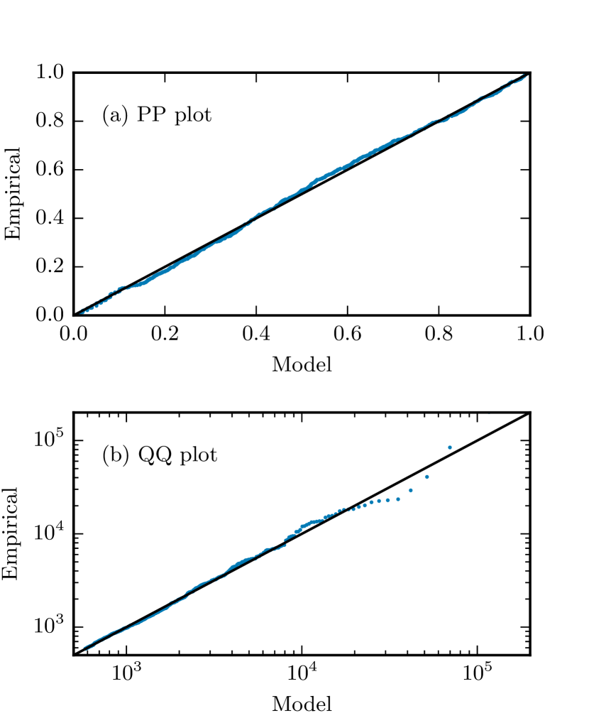
The goodness of the model fit can be graphically checked with PP and QQ plots. Given an ordered sample of independent observations
the empirical distribution function is defined by
Suppose is an estimated distribution function of , then a probability plot, also called PP plot, consists of the points
| (14) |
and a quantile plot, also called QQ plot, consists of the points
| (15) |
where is the estimated quantile function (Coles, 2001, p.36). If is a good estimate of the distribution function , then the points in a QQ plot and in a PP plot should lie close to the unit diagonal. An example is shown in Fig. 12. QQ plots turned out to much more sensitive about the threshold choice than PP plots. All PP and QQ plots show that the estimated model agrees excellently with the data.
VI Running mean
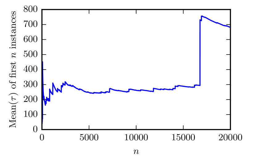
In the main paper we show that the tail of the distribution of for SQA is always heavy () for problems with spins. Sometimes the estimated shape parameter is even indicating that the mean of the GP distribution function is infinite but, as there exists only a finite number of instances, the mean of the distribution function of is not divergent but dominated by the hardest instances. This can easily be seen by considering the running mean of , i.e. the mean of for the first instances. See Fig. 13 which shows that the mean is not converging using 20000 random instances with 288 spins for SQA with and optimal annealing time . This is expected because the estimated shape parameter is .
VII DATA
Here we show the results of the tail analysis and repeat the necessary details from the main text in order to be self-contained in the presentation of the data.
For every algorithm, schedule and system size we used 20000 random instances to estimate for each instance the single-run success probability to find the ground state by averaging over many repetitions. Then the mean number of repetitions required to find the ground state is calculated. The distribution function is analyzed using extreme value theory: The exceedances over a high threshold are fitted to a GP distribution function, such that . In the tables below are the results for SA, SQA and MFA: is the number of spins, is the threshold, are the number of threshold exceedances, i.e. the number of instances that have from all the 20000 instances, is the estimated shape parameter and is the estimated scale parameter of the GP distribution function . Both and are shown with the standard error obtained from the maximum likelihood estimation method.
| 32 | 200 | 12.9 | ||
| 72 | 1000 | 21.3 | ||
| 128 | 1000 | 37.0 | ||
| 200 | 1000 | 58.4 | ||
| 288 | 998 | 165 | ||
| 392 | 998 | 317 | ||
| 512 | 400 | 1208 |
| 32 | 194 | 1.5 | ||
| 72 | 599 | 2.4 | ||
| 128 | 400 | 5.8 | ||
| 200 | 1000 | 8.6 | ||
| 288 | 999 | 20.1 | ||
| 392 | 599 | 79.0 | ||
| 512 | 399 | 373 |
| 32 | 200 | 1.6 | ||
| 72 | 200 | 26.0 | ||
| 128 | 400 | 113 | ||
| 200 | 400 | 1381 | ||
| 288 | 318 | 36281 |
| 32 | 400 | 7.9 | ||
| 72 | 200 | 23.2 | ||
| 128 | 400 | 47.3 | ||
| 200 | 400 | 219 | ||
| 288 | 1000 | 603 |
| 32 | 400 | 6.5 | ||
| 72 | 400 | 15.7 | ||
| 128 | 398 | 48.3 | ||
| 200 | 200 | 318 | ||
| 288 | 400 | 648 |
| 32 | 400 | 7.6 | ||
| 72 | 198 | 42.4 | ||
| 128 | 398 | 140 | ||
| 200 | 400 | 226 | ||
| 288 | 400 | 998 | ||
| 392 | 198 | 9302 |
| 32 | 298 | 23.5 | ||
| 72 | 398 | 54.5 | ||
| 128 | 100 | 256 | ||
| 200 | 398 | 459 | ||
| 288 | 399 | 3419 |