Local quantum thermal susceptibility

Abstract

Thermodynamics relies on the possibility to describe systems composed of a large number of constituents in terms of few macroscopic variables. Its foundations are rooted into the paradigm of statistical mechanics, where thermal properties originate from averaging procedures which smoothen out local details. While undoubtedly successful, elegant and formally correct, this approach carries over an operational problem: what is the precision at which such variables are inferred, when technical/practical limitations restrict our capabilities to local probing? Here we introduce the local quantum thermal susceptibility, a quantifier for the best achievable accuracy for temperature estimation via local measurements. Our method relies on basic concepts of quantum estimation theory, providing an operative strategy to address the local thermal response of arbitrary quantum systems at equilibrium. At low temperatures it highlights the local distinguishability of the ground state from the excited sub-manifolds, thus providing a method to locate quantum phase transitions.

The measurement of temperature is a key aspect in science, technology, and in our daily life. Many ingenious solutions have been designed to approach different situations and required accuracies Pekola . What is the ultimate limit to the precision at which the temperature of a macroscopic state can be determined? An elegant answer to this question is offered by estimation theory cramer ; paris_book ; paris1 : The precision is related to the heat capacity of the system zanardi_heatcapacity1 ; zanardi_heatcapacity2 .

In view of the groundbreaking potentialities offered by present-day nanotechnologies gao ; nano1 ; nano2 ; nano3 ; thermo_exp ; thermo_exp1 and the need to control the temperature at the nano-scale, it is highly relevant to question whether the heat capacity is still the relevant (fundamental) precision limit to small-scale thermometry. The extensivity of the heat capacity is a consequence of the growing volume-to-surface ratio with the size Huang . However, at a microscopic level such construction may present some limitations Hill ; Hill1 . Moreover a series of theoretical efforts recently concentrated on a self-consistent generalization of the classical thermodynamics to small-scale physics, where quantum effects become predominant gemmer ; Allahverdyan ; Allahverdyan1 ; Nieuwenhuizen ; Lutz ; LeHur ; Horodecki . In particular, a lot of attention has been devoted to the search for novel methods of precision nanothermometry that could exploit the essence of quantum correlations Qest_JC ; Qest_JC2 ; marzolino ; thermo_theory ; mandarino ; thermo_theory_XYmodel . In this context, the possibility to correctly define the thermodynamical limit, and therefore the existence of the temperature in the quantum regime, has been thoroughly investigated. It has been shown that the minimal subset of an interacting quantum system which can be described as a canonical ensemble, with the same temperature of the global system, depends not only on the strength of the correlations within the system, but also on the temperature itself hartmann1 ; hartmann1b ; hartmann2 . Using a quantum information-oriented point of view, this phenomenon has been also highlighted in Gaussian fermionic and bosonic states, by exploiting quantum fidelity as the figure of merit saez ; saez2 . Furthermore, the significant role played by quantum correlations has been recently discussed with specific attention to spin- and fermonic-lattice systems with short-range interactions eisert .

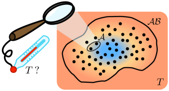
In this paper we propose a quantum-metrology approach to thermometry, through the analysis of the local sensitivity of generic quantum systems to their global temperature. Our strategy does not assume any constraint neither on the structure of the local quantum state, nor on the presence of strong quantum fluctuations within the system itself, while it rather moves from the observation that the temperature is a parameter which can be addressed only via indirect measurements. Specifically we introduce a new quantity which we dub Local Quantum Thermal Susceptibility (LQTS), and which gauges how efficiently the thermal equilibrium of a system is perceived by its subparts. More precisely, given a quantum system ${\cal AB}$ in a thermal equilibrium state, the LQTS $\mathfrak{S}_{\cal A}$ is a response functional which quantifies the highest achievable accuracy for estimating the system temperature $T$ through local measurements performed on a selected subsystem ${\cal A}$ of ${\cal AB}$ (see Fig. 1).

Figure 1: The operationally grounded strategy associated to the LQTS functional. A composite quantum system $\cal S$ is in thermal equilibrium with a bath at temperature $T$. The LQTS functional (1) measures the highest achievable accuracy in the estimation $T$ under the hypothesis to perform only local measurements on the subsystem $\cal A$ of ${\cal AB}$.

The LQTS is in general not extensive with respect to the size of ${\cal A}$, yet it is an increasing function of the latter, and it reduces to the system heat capacity in the limit where the probed part coincides with the whole system ${\cal AB}$. In the low-temperature limit, we shall also see that the LQTS is sensitive to the local distinguishability between the ground state and the first excited subspace of the composite system Hamiltonian. In this regime, even for a tiny size of the probed subsystem, our functional is able to predict the behaviour of the heat capacity and in particular to reveal the presence of critical regions. This naturally suggests the interpretation of $\mathfrak{S}_{\cal A}$ as a sort of mesoscopic version of the heat capacity which replaces the latter in those regimes where extensivity breaks down.

I Results

The functional.

Let us consider a bipartite quantum system ${\cal AB}$ at thermal equilibrium, composed of two subsystems ${\cal A}$ and ${\cal B}$, and described by the canonical Gibbs ensemble $\rho_{\beta}=e^{-\beta H}/{\cal Z}_{\beta}$. Here $H=H_{\cal A}+H_{\cal B}+H_{\cal AB}^{\rm(int)}$ is the system Hamiltonian, which in the general case will include both local (i.e., $H_{\cal A}$ and $H_{\cal B}$) and interaction (i.e., $H_{\cal AB}^{\rm(int)}$) terms, while ${\cal Z}_{\beta}=\mathrm{Tr}[e^{-\beta H}]=\sum_{i}e^{-\beta E_{i}}$ denotes the associated partition function ($\beta=1/k_{B}T$ is the inverse temperature of the system, $k_{B}$ the Boltzmann constant, and $\{E_{i}\}$ the eigenvalues of $H$). In this scenario we are interested in characterizing how the actual temperature $T$ is perceived locally on ${\cal A}$.

For this purpose we resort to quantum metrology giovannetti and define the LQTS of subsystem ${\cal A}$ as

$$\mathfrak{S}_{\cal A}[\rho_{\beta}]:=8\lim_{\varepsilon\to 0}\frac{1-\mathcal{F}\big{(}\rho^{\cal A}_{\beta},\rho^{\cal A}_{\beta+\varepsilon}\big{)}}{\varepsilon^{2}}\,,$$ (1)

where $\mathcal{F}\left(\rho,\sigma\right)=\mathrm{Tr}[\sqrt{\sqrt{\rho}\,\sigma\sqrt{\rho}}]$ is the fidelity between two generic quantum states $\rho$ and $\sigma$ peres ; jozsa . The quantity (1) corresponds to the quantum Fisher information (QFI) paris_book ; paris1 for the estimation of $\beta$, computed on the reduced state $\rho^{\cal A}_{\beta}=\mathrm{\mathrm{Tr}missing}_{\mathcal{B}}[\rho_{\beta}]$. It gauges how modifications on the global system temperature are affecting ${\cal A}$, the larger being $\mathfrak{S}_{\cal A}[\rho_{\beta}]$ the more sensitive being the subsystem response. More precisely, through the quantum Cramér-Rao inequality, $\mathfrak{S}_{\cal A}[\rho_{\beta}]$ quantifies the ultimate precision limit to estimate the temperature $T$, by means of any possible local (quantum) measurement on subsystem ${\cal A}$. In the specific, it defines an asymptotically achievable lower bound,

$${\Delta T}^{\cal A}\geq k_{B}T^{2}/\sqrt{N\mathfrak{S}_{\cal A}[\rho_{\beta}]}\,,$$ (2)

on the root-mean-square error ${\Delta T}^{\cal A}=\sqrt{\mathbb{E}[(T^{\mathrm{est}}-T)^{2}]}$ of a generic local estimation strategy, where $T^{\mathrm{est}}$ is the estimated value of $T$, $\mathbb{E}[x]$ is the expectation value for a random variable $x$, and $N$ is the number of times the local measurement is repeated.

By construction, $\mathfrak{S}_{\cal A}[\rho_{\beta}]$ is a positive quantity which diminishes as the size of ${\cal A}$ is reduced, the smaller being the portion of the system we have access to, the worse being the accuracy we can achieve. More precisely, given ${\cal A}^{\prime}$ a proper subset of ${\cal A}$, we have $\mathfrak{S}_{{\cal A}^{\prime}}[\rho_{\beta}]\leq\mathfrak{S}_{\cal A}[\rho_{\beta}]$. In particular, when ${\cal A}$ coincides with the whole system ${\cal AB}$, equation (1) reaches its maximum value and becomes equal to the variance of the energy,

$$\mathfrak{S}_{\cal AB}[\rho_{\beta}]=\mathrm{Tr}[\rho_{\beta}H^{2}]-\mathrm{Tr}[\rho_{\beta}H]^{2}\,,$$ (3)

which depends only on the spectral properties of the system and which coincides with the system heat capacity zanardi_heatcapacity1 ; zanardi_heatcapacity2 (note that, rigorously speaking, the LQTS quantifies the sensitivity of the system to its inverse temperature $\beta$; the corresponding susceptibility to $T=1/(k_{B}\beta)$ gets a $k_{B}^{-2}T^{-4}$ correction term, which also enters the standard definition of the heat capacity).

An explicit evaluation of the limit in equation (1) can be obtained via the Uhlmann’s theorem uhlmann (see Methods for details). A convenient way to express the final result can be obtained by introducing an ancillary system ${\cal A^{\prime}B^{\prime}}$ isomorphic to ${\cal AB}$ and the purification of $\rho_{\beta}$ defined as

$$|\rho_{\beta}\rangle=\sum_{i}\frac{e^{-\beta E_{i}/2}}{\sqrt{{\cal Z}_{\beta}}}|E_{i}\rangle_{\cal A\cal B}\otimes|E_{i}\rangle_{\cal A^{\prime}\cal B^{\prime}}\;,$$ (4)

where $H\!=\!\sum_{i}\!E_{i}|E_{i}\rangle_{\cal A\cal B}\langle E_{i}|$ is the spectral decomposition of the system Hamiltonian. It can then be proved that

$$\mathfrak{S}_{\cal A}[\rho_{\beta}]=\mathfrak{S}_{\cal AB}[\rho_{\beta}]-\sum_{j<k}\frac{(\lambda_{j}-\lambda_{k})^{2}}{\lambda_{j}+\lambda_{k}}|\langle e_{k}|H|e_{j}\rangle|^{2}\,,$$ (5)

where $\{|e_{j}\rangle\}$ are the eigenvectors of the reduced density matrix $\mathrm{Tr}_{\cal A^{\prime}}[|\rho_{\beta}\rangle\langle\rho_{\beta}|]$ living on ${\cal ABB^{\prime}}$, obtained by taking the partial trace of $|\rho_{\beta}\rangle$ with respect to the ancillary system ${\cal A^{\prime}}$, while $\{\lambda_{j}\}$ are the corresponding eigenvalues (which, by construction, coincide with the eigenvalues of $\rho_{\beta}^{\cal A}$).

Equation (5) makes it explicit the ordering between $\mathfrak{S}_{\cal A}[\rho_{\beta}]$ and $\mathfrak{S}_{\cal AB}[\rho_{\beta}]$: the latter is always greater than the former due to the negativity of the second contribution appearing on the rhs. Furthermore, if $H$ does not include interaction terms (i.e., $H_{\cal AB}^{\rm(int)}=0$), one can easily verify that $\mathfrak{S}_{\cal A}[\rho_{\beta}]$ reduces to the variance of the local Hamiltonian of ${\cal A}$, and is given by the heat capacity of the Gibbs state $e^{-\beta H_{\cal A}}/{\cal Z}^{\cal A}_{\beta}$ which, in this special case, represents $\rho_{\beta}^{\cal A}$, i.e., $\mathfrak{S}_{\cal A}[\rho_{\beta}]=\mathrm{Tr}[\rho^{\cal A}_{\beta}H_{\cal A}^{2}]-\mathrm{Tr}[\rho^{\cal A}_{\beta}H_{\cal A}]^{2}=-\frac{\partial^{2}}{\partial\beta^{2}}\ln{\cal Z}^{\cal A}_{\beta}$. Finally we observe that in the high-temperature regime ($\beta\to 0$) the expression (5) simplifies yielding

$$\mathfrak{S}_{\cal A}[\rho_{\beta}]\!=\!\frac{1}{d_{\cal A}}\mathrm{Tr}\!\!\left[\tilde{H}_{\cal A}^{2}-2\beta\tilde{H}_{\cal A}\frac{\mathrm{Tr}_{\cal B}[H^{2}]}{d_{\cal B}}+\beta\tilde{H}_{\cal A}^{3}\right]\!+\mathcal{O}(\beta^{2})\,,$$ (6)

where $d_{\cal A}$ and $d_{\cal B}$ denote the Hilbert space dimensions of ${\cal A}$ and ${\cal B}$ respectively, and we defined $\tilde{H}_{\cal A}=\mathrm{Tr}_{\cal B}[H]/d_{\cal B}$ having set, without loss of generality, $\mathrm{Tr}[H]=0$.

Figure 2: Schematic representation of the low-energy spectrum for a generic many-body quantum system. For simplicity the ground-state (gs) energy $E_{0}$ is set to zero. Here $\Pi_{i}$ denotes the normalized projector on the eigenspaces of energy $E_{i}$, which can be $n_{i}$-fold degenerate.

A measure of state distinguishability.

In the low-temperature regime, the LQTS can be used to characterize how much the ground state of the system ${\cal AB}$ differs from the first excited subspaces when observing it locally on ${\cal A}$. This is a direct consequence of the fact that the QFI (which we used to define our functional) accounts for the degree of statistical distinguishability between two quantum states (in our case the reduced density matrices $\rho_{\beta}^{\cal A}$ and $\rho_{\beta+\varepsilon}^{\cal A}$) differing by an infinitesimal change in the investigated parameter (in our case the inverse temperature $\beta$). Therefore for $\beta\to\infty$, the LQTS can be thought as a quantifier of the local distinguishability among the lowest energy levels in which the system is frozen.

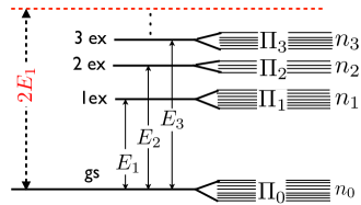
To clarify this point, let us consider the general scenario depicted in Fig. 2, where we only discuss the physics of the ground state (with energy $E_{0}=0$) and of the lowest excited levels with energy $E_{i}$ bounded by twice the energy of the first excited level, $E_{i}\leq 2E_{1}$. The degeneracy of each considered energy eigenstate is denoted by $n_{i}$. From equation (5) it then follows that up to first order in the parameter $e^{-\beta E_{1}}$ we get

$$\mathfrak{S}_{\cal A}[\rho_{\beta}]=\sum_{i}\frac{n_{i}}{n_{0}}E_{i}^{2}e^{-\beta E_{i}}\Big{(}1-\mathrm{Tr}[P_{0}^{\cal A}\Pi_{i}^{\cal A}]\Big{)}+\mathcal{O}\left(e^{-2\beta E_{1}}\right).$$ (7)

Here $\Pi_{i}^{\cal A}=\mathrm{Tr}_{\cal B}[\Pi_{i}]$, where $\Pi_{i}$ is the normalized projector on the degenerate subspace of energy $E_{i}$. Moreover, $P^{\cal A}_{0}$ is the span of the local subspace associated to the ground state, i.e., $P_{0}^{\cal A}=\sum_{j=1}^{n_{0}^{\cal A}}|\phi_{j}\rangle_{\cal A}\langle\phi_{j}|$, with $\Pi_{0}^{\cal A}=\sum_{j=1}^{n_{0}^{\cal A}}p_{j}|\phi_{j}\rangle_{\cal A}\langle\phi_{j}|$, and $n_{0}^{\cal A}$ being the number of non-zero eigenvalues ($p_{j}>0$) of $\Pi_{0}^{\cal A}$.

Equation (7) can be interpreted as follows. Our capability of measuring $\beta$ relies on the distinguishability between the states $\rho_{\beta}^{\cal A}$ and $\rho_{\beta+\varepsilon}^{\cal A}$, with $\varepsilon\ll\beta$. In the zero-temperature limit, the system lies in the ground state and locally reads as $\Pi_{0}^{\cal A}$, while at small temperatures the lowest energy levels start to get populated. If their reduced projectors $\Pi_{i}^{\cal A}$ ($i\geq 1$) are not completely contained in the span of $\Pi_{0}^{\cal A}$, that is $\mathrm{Tr}[P_{0}^{\cal A}\,\Pi_{i}^{\cal A}]\neq 1$, there exist some local states whose population is null for $T=0$ and greater than zero at infinitesimal temperatures. Such difference implies that the first order in $\mathfrak{S}_{\cal A}$ does not vanish. On the contrary, if the reduced projectors $\Pi_{i}^{\cal A}$ are completely contained in the span of $\Pi_{0}^{\cal A}$, that is $\mathrm{Tr}[P_{0}^{\cal A}\,\Pi_{i}^{\cal A}]=1$, we can distinguish $\rho_{\beta}^{\cal A}$ from $\rho_{\beta+\varepsilon}^{\cal A}$ only thanks to infinitesimal corrections $\mathcal{O}(\!\exp(-2\beta E_{1}))$ to the finite-valued populations of the lowest energy levels (see Methods for an explicit evaluation of the latter). In conclusion, the quantity $\mathfrak{S}_{\cal A}[\rho_{\beta\to\infty}]$ acts as a thermodynamical indicator of the degree of distinguishability between the ground-state eigenspace and the lowest energy levels in the system Hamiltonian.

LQTS and phase estimation.

A rather stimulating way to interpret equation (5) comes from the observation that, in the extended scenario where we have purified ${\cal AB}$ as in equation (4), the global variance (3) formally coincides with the QFI $\mathfrak{F}_{\cal ABA^{\prime}B^{\prime}}(|\rho_{\beta}^{(\varphi)}\rangle)$ associated with the estimation of a phase $\varphi$ which, for given $\beta$, has been imprinted into the system ${\cal ABA^{\prime}B^{\prime}}$ by a unitary transformation $e^{-iH^{\prime}\varphi/2}$, with $H^{\prime}$ being the analogous of $H$ on the ancillary system ${\cal A^{\prime}B^{\prime}}$, i.e., $\mathfrak{S}_{\cal AB}[\rho_{\beta}]=\mathfrak{F}_{\cal ABA^{\prime}B^{\prime}}(|\rho_{\beta}^{(\varphi)}\rangle)$ where $|\rho_{\beta}^{(\varphi)}\rangle=e^{-iH^{\prime}\varphi/2}|\rho_{\beta}\rangle$ paris1 ; giovannetti ; caves . Interestingly enough a similar connection can be also established with the second term appearing in the rhs of equation (5): indeed the latter coincides with the QFI $\mathfrak{F}_{\cal BA^{\prime}B^{\prime}}(|\rho_{\beta}^{(\varphi)}\rangle)$ which defines the Cramér-Rao bound for the estimation of the phase $\varphi$ of $|\rho_{\beta}^{(\varphi)}\rangle$, under the constraint of having access only on the subsystem ${\cal BA^{\prime}B^{\prime}}$ (i.e., that part of the global system which is complementary to ${\cal A}$). Accordingly we can thus express the LQTS as the difference between these two QFI phase estimation terms, the global one vs. the local one or, by a simple rearrangement of the various contributions, construct the following identity

$$\mathfrak{S}_{\cal A}[\rho_{\beta}]+\mathfrak{F}_{\cal BA^{\prime}B^{\prime}}(|\rho_{\beta}^{(\varphi)}\rangle)=\langle\Delta H^{2}\rangle_{\beta}\;,$$ (8)

which establishes a complementarity relation between the temperature estimation on ${\cal A}$ and the phase estimation on its complementary counterpart ${\cal BA^{\prime}B^{\prime}}$, by forcing their corresponding accuracies to sum up to the energy variance $\langle\Delta H^{2}\rangle_{\beta}$ of the global system (3).

Local thermometry in many-body systems.

We have tested the behaviour of our functional on two models of quantum spin chains, with a low-energy physics characterized by the emergence of quantum phase transitions (QPTs) belonging to various universality classes sachdev .

Figure 3: The LQTS in the Ising and the Heisenberg models at low temperature. We numerically computed the LQTS of equation (1) in the low-temperature limit for a chain with $L=12$ sites in the following two cases: (a) the Ising model as a function of the transverse field $h$; (b) the Heisenberg XXZ chain as a function of the anisotropy $\Delta$. The uppermost (red) curve corresponds to the global quantum thermal susceptibility, that is the heat capacity. The other curves stand for different sizes $n_{\cal A}$ of the measured subsystem ${\cal A}$ of ${\cal AB}$ ($n_{\cal A}$ increases along the direction of the arrow). The inset in panel (b) magnifies the data around $\Delta=-1$. In the XXZ model, the LQTS with $n_{\cal A}=1$ can be proved to rigorously vanish. The inverse temperature has been fixed in both cases at $\beta=9$.

Specifically, we consider the quantum spin-$1/2$ Ising and Heisenberg chains, in a transverse magnetic field $h$ and with a $z$-axis anisotropy $\Delta$ respectively,

$$H_{\rm Ising} \!=\! -J\sum_{i}\left[\sigma_{i}^{x}\sigma_{i+1}^{x}+h\sigma_{i}^{z}\right],$$ (9)

$$H_{\rm XXZ} \!=\! J\sum_{i}\left[(\sigma_{i}^{x}\sigma_{i+1}^{x}+\sigma_{i}^{y}\sigma_{i+1}^{y})\!+\!\Delta\,\sigma_{i}^{z}\sigma_{i+1}^{z}\right]\!.$$ (10)

Here $\sigma^{\alpha}_{i}$ denotes the usual Pauli matrices ($\alpha=x,y,z$) on the $i$th site, and periodic boundary conditions have been assumed. We set $J=1$ as the system’s energy scale. At zero temperature, the model (9) presents a $\mathbb{Z}_{2}$-symmetry breaking phase transition at $|h_{c}|=1$ belonging to the Ising universality class. The Hamiltonian (10) has a critical behaviour for $-1\leq\Delta\leq 1$, while it presents a ferromagnetic or antiferromagnetic ordering elsewhere. In the latter case, the system exhibits a first-order QPT in correspondence to the ferromagnetic point $\Delta_{\rm f}=-1$, and a continuous QPT of the Kosterlitz-Thouless type at the antiferromagnetic point $\Delta_{\rm af}=1$.

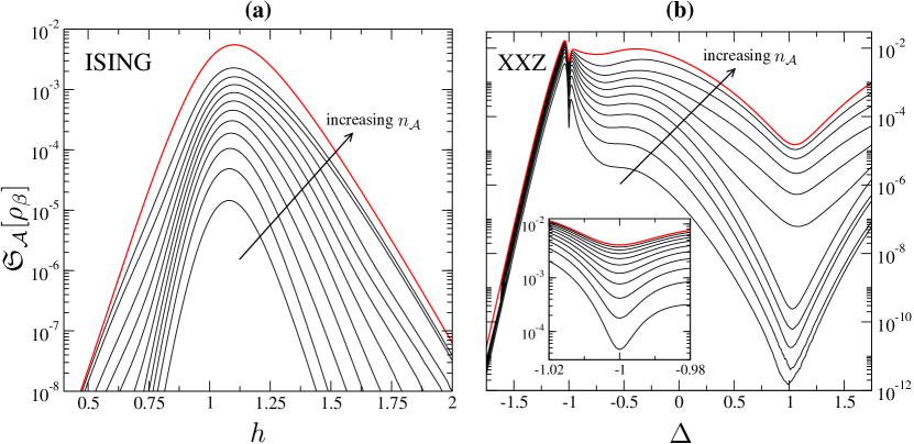
Figure 3 displays the small-temperature limit of $\mathfrak{S}_{\cal A}[\rho_{\beta}]$ for the two models above, numerically computed by exploiting expression (21) in Methods. We first observe that, as expected, for all the values of $h$ and $\Delta$ the LQTS monotonically increases with increasing the number $n_{\cal A}$ of contiguous spins belonging to the measured subsystem ${\cal A}$. More interestingly, we find that even when $\cal A$ reduces to two or three sites, its thermal behaviour qualitatively reproduces the same features of the global system (represented in both models by the uppermost curve). In particular, even at finite temperatures and for systems composed of twelve sites, the LQTS is sensitive to the presence of critical regions where quantum fluctuations overwhelm thermal ones. The reminiscence of QPTs at finite temperatures has been already discussed via a quantum-metrology approach, through the analysis of the Bures metric tensor in the parameter space associated to the temperature and the external parameters zanardiT . The diagonal element of such tensor referring to infinitesimal variations in temperature, corresponds to the thermal susceptibility of the whole system. The latter quantity has been recently studied for the XY model thermo_theory_XYmodel , showing its sensitivity to critical points of Ising universality class.

In the low-temperature regime such global sensitivity can be understood within the Landau-Zener (LZ) formalism LZ . This consists of a two-level system, whose energy gap $\Delta E$ varies with respect to an external control parameter $\Gamma$, and presents a minimum $\Delta E_{\rm min}$ in correspondence to some specific value $\Gamma_{c}$. Conversely, the global heat capacity (3) may exhibit a maximum or a local minimum at $\Gamma_{c}$, according to whether $\Delta E_{\rm min}$ is greater or lower than the value of $\Delta E^{\star}$ at which the expression $\mathfrak{S}_{\cal AB}[\rho_{\beta}]\equiv\langle\Delta H^{2}\rangle_{\beta}$ is maximum in $\Delta E$, respectively. Indeed it can be shown that $\langle\Delta H^{2}\rangle_{\beta}$ for a two-level system exhibits a non-monotonic behaviour as a function of $\Delta E$, at fixed $\beta$ (see Methods). Quite recently, an analogous mechanisms has been also pointed out for the global heat capacity in the Lipkin-Meshkov-Glick model mandarino . The LZ formalism represents a simplified picture of the mechanism underlying QPTs in many-body systems. However, by definition the temperature triggers the level statistics and the equilibrium properties of physical systems. Therefore, both the heat capacity of the global system zanardi_heatcapacity1 ; zanardi_heatcapacity2 and the LQTS of its subsystems are expected to be extremely sensitive to the presence of critical regions in the Hamiltonian parameter space.

We also performed a finite-size scaling analysis of $\mathfrak{S}_{\cal A}[\rho_{\beta}]$ as a function of the size of the measured subsystem. For slightly interacting systems, one expects the LQTS to be well approximated by the heat capacity of ${\cal A}$ (at least when this subsystem is large enough). The latter quantity should scale linearly with its size $n_{\cal A}$. This is indeed the case for the Ising model (9), where a direct calculation of $\langle\Delta H^{2}\rangle_{\beta}$ can be easily performed thermo_theory_XYmodel . Our data for the scaling of the stationary points of $\mathfrak{S}_{\cal A}[\rho_{\beta}]$ close to QPTs suggest that significant deviations from a linear growth with $n_{\cal A}$ are present (see the Supplementary Information). This indicates that correlations cannot be neglected for the sizes and the systems considered here.

II Discussion

We have proposed a theoretical approach to temperature locality based on quantum estimation theory. Our method deals with the construction of the local quantum thermal susceptibility, which operationally highlights the degree at which the thermal equilibrium of the global system is perceived locally, avoiding any additional hypothesis on the local structure of the system. This functional corresponds to the highest achievable accuracy up to which it is possible to recover the system temperature at thermal equilibrium via local measurements. Let us remark that, even if in principle the Cramér-Rao bound is achievable, from a practical perspective it represents a quite demanding scenario, as it requires the precise knowledge of the Hamiltonian, the possibility to identify and perform the optimal measurements on its subsystems, and eventually a large number of copies of the system. However, in this manuscript we have adopted a more theoretical perspective, and focused on the geometrical structure of the quantum statistical model underlying local thermalization.

In the low-temperature regime our functional admits an interpretation as a measure of the local state distinguishability between the spaces spanned by the Hamiltonian ground state and its first energy levels. Furthermore we established a complementarity relation between the highest achievable accuracy in the local estimation of temperature and of a global phase, by showing that the corresponding accuracies associated with complementarity subsystems sum up to heat capacity of the global system. Finally, we considered two prototypical many-body systems featuring quantum phase transitions, and studied their thermal response at low temperatures. On one hand, we found that optimal measurements on local systems provide reliable predictions on the global heat capacity. On the other hand, our functional is sensitive to the presence of critical regions, even though the total system may reduce to a dozen of components and the measured subsystem to one or two sites. Let us remark that most of the results presented herewith do not refer to any specific choice of the interaction Hamiltonian, $H_{\cal AB}^{\rm(int)}$ between $\cal A$ and $\cal B$. As an interesting implementation of our scheme, we foresee the case of non-thermalizing interactions stace ; zwierz , whose potentialities for precision thermometry have been already unveiled.

We conclude by noticing that, while in this article we focused on temperature, the presented approach can be extended to other thermodynamic quantities (like entropy, pressure, chemical potential etc.). Furthermore it seems plausible to adopt quantum estimation strategies to tackle the problem of providing self-consistent definition of heat and work for microscopic systems (see Ref. campisi and references therein). One of the main difficulties to this end derives indeed from the fact that these thermodynamic functionals are processes rather than state variables: accordingly there are no quantum observables associated with them. In this respect a quantum-estimation strategy not explicitly referred to a specific quantum observable, but rather bearing the geometrical traits of the Hilbert space associated to the explored systems, appears as a valid chance to close this gap.

III Methods

Derivation of equation (5).

Let us recall the definition of the LQTS for a given subsystem $\cal A$ of a global system $\cal S$ at thermal equilibrium:

$$\mathfrak{S}_{\cal A}[\rho_{\beta}]=8\lim_{\varepsilon\to 0}\frac{1-\mathcal{F}\big{(}\rho^{\cal A}_{\beta},\rho^{\cal A}_{\beta+\varepsilon}\big{)}}{\varepsilon^{2}}\,,$$ (11)

where $\mathcal{F}\left(\rho,\sigma\right)=\mathrm{Tr}[\sqrt{\sqrt{\rho}\,\sigma\sqrt{\rho}}]$ is the fidelity between two generic quantum states $\rho$ and $\sigma$. According to the Uhlmann’s theorem uhlmann , we can compute $\cal F$ as

$$\mathcal{F}\left(\rho^{\cal A}_{\beta},\rho^{\cal A}_{\beta+\varepsilon}\right)=\max_{|\rho^{\cal A}_{\beta}\rangle,|\rho^{\cal A}_{\beta+\varepsilon}\rangle}|\langle\rho^{\cal A}_{\beta}|\rho^{\cal A}_{\beta+\varepsilon}\rangle|,$$ (12)

where the maximization involves all the possible purifications $|\rho^{\cal A}_{\beta}\rangle$ and $|\rho^{\cal A}_{\beta+\varepsilon}\rangle$ of $\rho^{\cal A}_{\beta}$ and $\rho^{\cal A}_{\beta+\varepsilon}$ respectively through an ancillary system $a$. A convenient choice is to set $a={\cal BA^{\prime}B^{\prime}}$, with ${\cal A^{\prime}B^{\prime}}$ isomorphic to ${\cal AB}$. We then observe that, by construction, the vector $|\rho_{\beta}\rangle$ of equation (4), besides being a purification of $\rho_{\beta}$, is also a particular purification of $\rho^{\cal A}_{\beta}$. We can now express the most generic purification of the latter as

$$|\rho^{\cal A}_{\beta}\rangle=(\openone_{\cal{A}}\otimes V)|\rho_{\beta}\rangle=(\openone_{\cal{A}}\otimes V)\frac{e^{-\beta H/2}}{\sqrt{{\cal Z}_{\beta}}}|\openone_{E}\rangle\,,$$ (13)

where $V$ belongs to the set of unitary transformations on $a$, where $\openone_{\cal X}$ represents the identity operator on the system ${\cal X}$, and where in the last equality we introduced the vector $|\openone_{E}\rangle=\sum_{i}|E_{i}\rangle_{\cal A\cal B}|E_{i}\rangle_{\cal A^{\prime}\cal B^{\prime}}$, $|E_{i}\rangle_{\cal AB}$ being the eigenvectors of $H$. We can thus write the fidelity (12) as

$$\mathcal{F}=\sqrt{\frac{\cal Z_{\beta}}{\cal Z_{\beta+\varepsilon}}}\max_{V}\Big{|}\langle\rho_{\beta}|\big{[}(\openone_{\cal{A}}\otimes V)\big{(}e^{-\varepsilon H/2}\otimes\openone_{\cal A^{\prime}\cal B^{\prime}}\big{)}\big{]}|\rho_{\beta}\rangle\Big{|}\,.$$ (14)

Since we are interested in the small-$\varepsilon$ limit, without loss of generality we set $V=\exp(i\,\varepsilon\,\Omega)$, with $\Omega$ being an Hermitian operator on the ancillary system $a$. It comes out that, up to corrections of order $\mathcal{O}(\varepsilon^{3})$, the LQTS reads

$$\mathfrak{S}_{\cal A}[\rho_{\beta}]=\mathfrak{S}_{\cal AB}[\rho_{\beta}]+4\min_{\Omega}\Big{\{}\mathrm{Tr}[\rho_{\beta}^{a}\Omega^{2}]-\mathrm{Tr}[\rho_{\beta}^{a}\Omega]^{2}$$

$$+\frac{i}{2}\langle\rho_{\beta}|[\Omega,H]|\rho_{\beta}\rangle\Big{\}}\,,$$ (15)

where we have defined $\rho_{\beta}^{a}=\mathrm{Tr}_{\cal A}[|\rho_{\beta}\rangle\langle\rho_{\beta}|]$. By differentiating the trace with respect to $\Omega$ we determine the minimization condition for it, yielding

$$(\Omega-\omega)\rho_{\beta}^{a}+\rho_{\beta}^{a}(\Omega-\omega)=Q\,,$$ (16)

with $\omega=\mathrm{Tr}[\rho_{\beta}^{a}\Omega]$ and $Q=-\frac{i}{2}\big{[}H^{\prime},\rho_{\beta}^{a}\big{]}$, $H^{\prime}$ being the analogous of $H$ which acts on ${\cal A^{\prime}B^{\prime}}$ (by construction $H|\rho_{\beta}\rangle=H^{\prime}|\rho_{\beta}\rangle$). Equation (16) explicitly implies that $\Omega$ does not depend on $\omega$, which, without loss of generality, can be set to zero. Moreover, it enables to rewrite the LQTS in equation (15) as

$$\mathfrak{S}_{\cal A}[\rho_{\beta}]=\mathfrak{S}_{\cal AB}[\rho_{\beta}]-4\,\mathrm{Tr}[\rho_{\beta}^{a}\,\Omega^{2}]\,.$$ (17)

The solution of the operatorial equation (16) can be found by applying the Lemma presented at the end of this section, yielding

$$\Omega = \Omega_{0}+\frac{i}{2}\left(PH^{\prime}R+RH^{\prime}P\right)$$ (18)

$$+\frac{i}{2}\left[\sum_{n=1}^{+\infty}(-1)^{n}\left(P{\rho_{\beta}^{a}}^{\circleddash n}H^{\prime}{\rho_{\beta}^{a}}^{n}-h.c.\right)\right]$$

with $\Omega_{0}$ being an operator which anti-commutes with $\Omega$, ${\rho_{\beta}^{a}}^{\circleddash m}$ being the Moore-Penrose pseudoinverse of $\rho_{\beta}^{a}$ to the power $m$, while $R$ being the projector on kernel of $\rho_{\beta}^{a}$, and $P=\openone_{a}-R$ being is complementary counterpart. By substituting this expression in equation (17), we finally get

$$\mathfrak{S}_{\cal A}[\rho_{\beta}]=2\sum_{j,k}\frac{\lambda_{j}\lambda_{k}}{\lambda_{j}+\lambda_{k}}|\langle e_{k}|H^{\prime}|e_{j}\rangle|^{2}-\mathrm{Tr}[\rho_{\beta}H]^{2}\,,$$ (19)

where $\rho_{\beta}^{a}=\sum_{i}\lambda_{i}|e_{i}\rangle\langle e_{i}|$ is the spectral decomposition of $\rho_{\beta}^{a}$, sharing the same spectrum with $\rho_{\beta}^{\cal A}$. The expression above holds for both invertible and not invertible $\rho_{\beta}^{a}$. To the latter scenario belongs the case in which $H=H_{\cal A}+H_{\cal B}$, where one can easily prove that the LQTS reduces to the variance of the local Hamiltonian $H_{\cal A}$, i.e. $\mathfrak{S}_{\cal A}=\mathrm{Tr}[\rho_{\beta}H_{\cal A}^{2}]-\mathrm{Tr}[\rho_{\beta}H_{\cal A}]^{2}$ (notice that the non-zero eigenvalues of $\rho_{\beta}^{a}$ are $\lambda_{i}=e^{-\beta E_{i}^{\cal A}}/{\cal Z}_{\beta}^{\cal A}$ which correspond to $|e_{i}\rangle=|E_{i}^{\cal A}\rangle\otimes|\rho_{\beta}^{\cal B}\rangle$, being $H_{\cal A}=\sum_{i}E_{i}^{\cal A}|E_{i}^{\cal A}\rangle\langle E_{i}^{\cal A}|$, ${\cal Z}_{\beta}^{\cal A}=\mathrm{Tr}[e^{-\beta H_{\cal A}}]$ and $|\rho_{\beta}^{\cal B}\rangle$ the purification of $\rho_{\beta}^{\cal B}$ through the ancillary system $\cal{B^{\prime}}$). The expression above can be also rewritten as

$$\mathfrak{S}_{\cal A}[\rho_{\beta}]=\mathfrak{S}_{\cal AB}[\rho_{\beta}]-\sum_{j<k}\frac{(\lambda_{j}-\lambda_{k})^{2}}{\lambda_{j}+\lambda_{k}}|\langle e_{k}|H^{\prime}|e_{j}\rangle|^{2}\,,$$ (20)

which can be cast into equation (5) by simply exploiting the fact that the system is symmetric with respect to the exchange of ${\cal AB}$ with ${\cal A^{\prime}B^{\prime}}$.

It is finally useful to observe that LQTS can be also expressed in terms of the eigenvectors of ${\cal A}$, $\rho_{\beta}^{\cal A}=\sum_{i}\lambda_{i}|g_{i}\rangle\langle g_{i}|$ as:

$$\mathfrak{S}_{\cal A}[\rho_{\beta}]=2\sum_{j,k}\frac{|\mathrm{Tr}[\rho_{\beta}H|g_{j}\rangle\langle g_{k}|]|^{2}}{\lambda_{j}+\lambda_{k}}-\mathrm{Tr}[\rho_{\beta}H]^{2},$$ (21)

where we have used the Schmidt decomposition of $|\rho_{\beta}\rangle$, with respect to bipartition ${\cal A}a$,

$$|\rho_{\beta}\rangle=\sum_{i}\sqrt{\lambda_{i}}|g_{i}\rangle|e_{i}\rangle.$$ (22)

In particular, expression (21) can be exploited in order to numerically compute the LQTS, for instance when dealing with quantum many-body systems (see Fig. 3 and the discussion in the Supplementary Information).

Lemma.

For any assigned operators $X,Y$ satisfying the equation

$$XW+WX=Y\,,$$ (23)

admit solutions of the form

$$W = W_{0}+X^{\circleddash 1}YR+RYX^{\circleddash 1}$$ (24)

$$+\sum_{n=0}^{+\infty}(-1)^{n}X^{n}PY(X^{\circleddash(n+1)}-R)\,,$$

where $X^{\circleddash 1}$ is the Moore Penrose pseudoinverse of $X$, $R$ is the projector on kernel of $X$, $P=\mbox{\rm\openone}-R$ ($\openone$ indicates the identity matrix) and $W_{0}$ is an generic operator which anti-commutes with $Y$. Furthermore if $X$ and $Y$ are Hermitian, equation (23) admits solutions which are Hermitian too: the latter can be expressed as

$$W = W_{0}+X^{\circleddash 1}YR+RYX^{\circleddash 1}$$

$$+\frac{1}{2}\bigg{[}\sum_{n=0}^{+\infty}(-1)^{n}X^{n}PY(X^{\circleddash(n+1)}-R)+h.c.\bigg{]},$$

where now $W_{0}$ is an arbitrary Hermitian operator which anti-commutes with $Y$.

Proof.

Since (23) is a linear equation, a generic solution can be expressed as the sum of a particular solution plus a solution $W_{0}$ of the associated homogeneous equation, i.e. an operator which anti-commute with $X$,

$$XW_{0}+W_{0}X=0\,.$$ (26)

A particular solution $W$ of equation (23) can be always decomposed as

$$W=RWR+RWP+PWR+PWP\,.$$ (27)

Notice that by definition $RX=XR=O$, where $O$ identifies the null operator. Multiplying (23) on both sides by $R$, one gets the condition $RYR=O$. The operator $W$, solution of equation (23), is defined up to its projection on the kernel subspace, that is

$$W^{\prime}=W+RWR\implies XW^{\prime}+W^{\prime}X=Y\,.$$ (28)

Therefore, without loss of generality we can set

$$RWR=O\,.$$ (29)

Multiplying equation (23) by $X^{\circleddash 1}$ on the right side and repeating the same operation on the left side we get:

$$RWP = RYX^{\circleddash 1}\,,$$ (30)

$$PWR = X^{\circleddash 1}YR\,.$$ (31)

On the other hand, $PWP$ satisfies the relation

$$PWP=PYX^{\circleddash 1}-PYR-X(PWP)X^{\circleddash 1}\,.$$ (32)

This equation can be solved recursively in $PWP$ and gives

$$PWP=\sum_{n=0}^{\infty}(-1)^{n}X^{n}PY(X^{\circleddash(1+n)}-R)\,,$$ (33)

thus concluding the first part of the proof. The second part of the proof follows simply by observing that, if $X$ and $Y$ are Hermitian, and if $W$ solves equation (23), then also its adjoint counterpart does. Therefore for each solution $W$ of the problem we can construct an Hermitian one by simply taking $(W+W^{\dagger})/2$. ∎

Second-order term corrections to LQTS.

In the low-temperature regime ($\beta\rightarrow\infty$), we have computed the second-order correction term to the LQTS, that is of $\mathfrak{S}_{\cal A}[\rho_{\beta}]$ in equation (1), and found:

$$\bigg{(}\!\!\frac{E_{1}n_{1}}{n_{0}}\!\!\bigg{)}^{\!2}\!e^{-2\beta E_{1}}\bigg{\{}\!\!-\!2\!+\!\mathrm{Tr}[P_{0}^{\cal A}\Pi_{1}^{\cal A}+\Pi_{1}^{\cal A}{\Pi_{0}^{\cal A}}^{\circleddash 1}\Pi_{1}^{\cal A}(1+P_{0}^{\cal A})]$$

$$-\!2\sum_{n=0}^{+\infty}(-1)^{n}\mathrm{Tr}\left[\Pi_{1}^{\cal A}{\Pi_{0}^{\cal A}}^{\circleddash(n+2)}\Pi_{1}^{\cal A}{\Pi_{0}^{\cal A}}^{n+1}\right]\!\bigg{\}}\;,$$

with $E_{k}\geq E_{1}$ and where the series in $n$ is meant to converge to $1/2$ when $\mathrm{Tr}\left[\Pi_{1}^{\cal A}{\Pi_{0}^{\cal A}}^{\circleddash(n+2)}\Pi_{1}^{\cal A}{\Pi_{0}^{\cal A}}^{n+1}\right]=1$, i.e., $\sum_{n=0}^{+\infty}(-1)^{n}\equiv\lim_{x\to-1}\sum_{n=0}^{+\infty}x^{n}=\frac{1}{2}$. In order to vanish, this second-order correction term requires a stronger condition with respect to one necessary to nullify the first-order term in the LQTS, equation (7). It is given by $\Pi_{1}^{\cal A}=\Pi_{0}^{\cal A}$, and corresponds to the requirement that the system ground state must be locally indistinguishable from the first excited level.

Heat capacity in the 2-level Landau-Zener scheme.

Here we discuss the simplified case in which only the ground state (with energy $E_{0}$) and the first excited level (with energy $E_{1}$) of the global system Hamiltonian $H$ play a role. In particular, we are interested in addressing a situation where the ground-state energy gap $\Delta E\equiv E_{1}-E_{0}$ may become very small, as a function of some external control parameter $\Gamma$ (e.g., the magnetic field or the system anisotropy). A sketch is depicted in Fig. 4, and refers to the so called Landau-Zener (LZ) model LZ . This resembles the usual scenario when a given many-body system is adiabatically driven, at zero temperature, across a quantum phase transition point.

Figure 4: The two-level Landau-Zener model. A sketch of the behaviour of the two eigenenergies $(E_{1},E_{2})$ as a function of some control parameter $\Gamma$. The gap $\Delta E=E_{2}-E_{1}$ displays a pronounced minimum in correspondence of a given $\Gamma^{c}$ value.

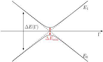
In correspondence of some critical value $\Gamma_{c}$, the gap is minimum. For a typical quantum many-body system, such minimum value $\Delta E_{\rm min}$ tends to close at the thermodynamic limit and a quantum phase transition occurs (notice that $\Gamma_{c}$ may depend on the system size). Hereafter, without loss of generality, we will assume $E_{0}=0$ and take $E_{1}=\Delta E$ so that the system heat capacity (3) reduces to:

$$\mathfrak{S}_{\cal AB}[\rho_{\beta}]=\frac{n_{1}(\Delta E)^{2}e^{-\beta\,\Delta E}}{n_{0}+n_{1}\,e^{-\beta\,\Delta E}}-\left(\frac{n_{1}\,\Delta E\,e^{-\beta\,\Delta E}}{n_{0}+n_{1}\,e^{-\beta\,\Delta E}}\right)^{2}\,.$$ (34)

Here $n_{0}$ and $n_{1}$ are the degeneracy indexes associated to the levels $E_{0}$ and $E_{1}$, respectively. Notice that $\mathfrak{S}_{\cal AB}[\rho_{\beta}]$ is always non-negative and exhibits a non-monotonic behaviour as a function of $\Delta E$, at fixed $\beta$. Indeed it is immediate to see that $\mathfrak{S}_{\cal AB}[\rho_{\beta}]\to 0$ in both limits $\Delta E\to 0$ and $\Delta E\to+\infty$. For fixed $\beta,n_{0}$ and $n_{1}$, the heat capacity displays a maximum in correspondence of the solution of the transcendental equation

$$\frac{\partial\mathfrak{S}_{\cal AB}[\rho_{\beta}]}{\partial\Delta E}=0\iff e^{\beta\,\Delta E}=\frac{n_{1}}{n_{0}}\frac{(2+\beta\,\Delta E)}{(\beta\,\Delta E-2)}.$$ (35)

In particular, for $n_{0}=n_{1}=1$ the latter relation is fulfilled for $\Delta E^{\star}\approx 2.3994/\beta$, while for $n_{0}=2,n_{1}=1$ it is fulfilled for $\Delta E^{\star}\approx 2.2278/\beta$.

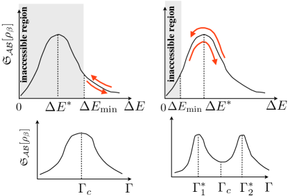
It turns out that the behaviour of the heat capacity as a function of increasing $\Gamma$ in a two-level LZ scheme depends on the relative sizes of $\Delta E^{\star}$ and $\Delta E_{\rm min}$, as pictorially shown in Fig. 5: a) if $\Delta E_{\rm min}>\Delta E^{\star}$, then $\mathfrak{S}_{\cal AB}[\rho_{\beta}]$ will exhibit a maximum in correspondence of $\Gamma_{c}$; b) if $\Delta E_{\rm min}<\Delta E^{\star}$, a maximum at $\Gamma_{1}^{\star}$ corresponding to $\Delta E=\Delta E^{\star}$ will appear, followed by a local minimum at $\Gamma_{c}$ and eventually by another maximum at $\Gamma_{2}^{\star}$ where the former condition occurs again. Since $\Delta E^{\star}$ is a function of $\beta$, and $\Delta E_{\rm min}$ depends on the system size, the point of minimum gap can be signaled by a maximum or by a local minimum depending on the way the two limits $L\to+\infty$ (thermodynamic limit) and $\beta\to+\infty$ (zero-temperature limit) are performed.

Figure 5: Heat capacity in the LZ model. The emergence of extremal points in the behaviour of $\mathfrak{S}_{\cal AB}[\rho_{\beta}]$ as a function of increasing control parameter $\Gamma$ is associated to the relative size of $\Delta E_{\rm min}$ with respect to $\Delta E^{*}$. The red arrows denote the changing of $\Delta E$ during a typical LZ protocol. One realizes that, if $\Delta E_{\rm min}>\Delta E^{*}$ one peak will appear (left), while if $\Delta E_{\rm min}<\Delta E^{*}$ one peaks will appear (right).

IV Acknowledgments

We thank G. Benenti and G. De Chiara for useful discussions. This work has been supported by MIUR through FIRB Projects RBFR12NLNA and PRIN “Collective quantum phenomena: from strongly correlated systems to quantum simulators”, by the EU Collaborative Project TherMiQ (Grant agreement 618074), and by the EU project COST Action MP1209 “Thermodynamics in the quantum regime”.

V Author contributions

All the authors conceived the work, agreed on the approach to pursue, analysed and discussed the results; A.D.P. performed the analytical calculations; D.R. performed the numerical calculations; V.G. and R.F. supervised the work.

VI Additional material

Supplementary Information

accompanies this paper below.

Competing financial interests:

The authors declare no competing financial interests.

.

VII Supplementary Information

VII.1 Scaling of the LQTS with the dimension $n_{\cal A}$
of subsystem ${\cal A}$.

The local quantum thermal susceptibility (LQTS) for the subsystem ${\cal A}$ of a given system, as defined in equation (1), is a quantity which is tricky to be evaluated numerically. Apart from the exponential growth of the Hilbert space, extrapolating the limit $\varepsilon\to 0$ typically requires high accuracies in the diagonalization procedure. This would generally limit the study of local thermometry in the many-body context up to very small systems. The expression that we derived in equation (21) circumvents the latter problem and enables an easier manipulation of $\mathfrak{S}_{\cal A}[\rho_{\beta}]$. However one still needs the full spectrum of the reduced density matrix $\rho_{\beta}^{\cal A}$, since all its eigenvectors have to be contracted with the product of the global equilibrium state times the system Hamiltonian, $\rho_{\beta}H$. This makes the whole analysis not straightforward, even for free-fermion systems as is the case for the Ising model $H_{\rm Ising}$. For this reason we resort to an exact diagonalization technique.

Figure 6: Peak value of $\mathfrak{S}_{\cal A}[\rho_{\beta}]$ for the Ising model, as a function of the dimension of the measured subsystem $n_{\cal A}$. Different data sets are for various system lengths $L$. The dashed line denotes a power-law behaviour $\mathfrak{S}_{\cal A}\sim(n/L)^{2}$, and is plotted as a guideline. The temperature is chosen as a function of the system size, as $\beta=3L/4$.

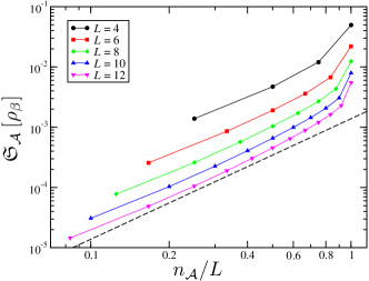
Let us concentrate on the scaling of the LQTS with the size $n_{\cal A}$ of the measured subsystem for the Ising spin chain (9). The maximum of $\mathfrak{S}_{\cal A}[\rho_{\beta}]$ as a function of $n_{\cal A}$, and for different system sizes $L$ is shown in Fig. 6. As noticed in the main text within the LZ discussion, the peak is related to the appearance of the critical point, but deviations from its position at the thermodynamic limit ($h_{c}=1$) are expected, due to the mutual interplay of finite-size and finite-temperature effects. To balance them, we choose a size-dependent temperature $\beta=3L/4$. While with exact diagonalization we cannot go beyond the study of systems with size $L=12$, our data suggest a power-law behaviour of the peak value at least for very small subsystems, scaling as

$$\mathfrak{S}_{\cal A}[\rho_{\beta}]\sim(n/L)^{\alpha},$$ (36)

with an exponent $\alpha\approx 2$.

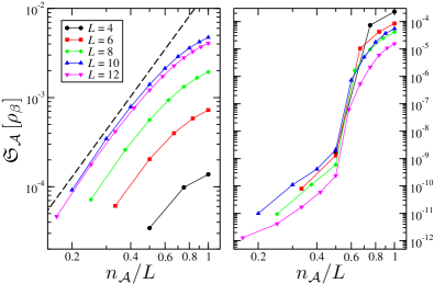
We performed the same analysis also for the XXZ chain (10), and focused on the behaviour of $\mathfrak{S}_{\cal A}[\rho_{\beta}]$ around the two critical points of the model, in correspondence to the two local minima. As we did above, we fix a size-dependent temperature $\beta=3L/4$ and study systems of size up to $L=12$. In the left panel of Fig. 7, we concentrate on the ferromagnetic point at $\Delta_{\rm f}=-1$. Similarly to the critical point of the Ising model, a power-law scaling of the type in equation (36) seems to emerge at small $n_{\cal A}$, with an exponent $\alpha\approx 3$. The scaling analysis at the antiferromagnetic point around $\Delta_{\rm af}=1$ is less clear and probably requires larger system sizes (right panel). We notice the appearance of a cusp-like feature at $n_{\cal A}=L/2$, which reflects the different behaviour of $\mathfrak{S}_{\cal A}[\rho_{\beta}]$ for $\Delta\approx\Delta_{\rm af}$, depending on whether $n_{\cal A}\leq L/2$ or $n_{\cal A}>L/2$, as is clearly visible in the right panel of Fig. 3. We have to stress that the departure of the two bunches of curves becomes more evident at large values of $\beta$, while it tends to disappear when increasing the temperature.

Figure 7: Same quantity and parameters as in Fig. 6, but for the XXZ chain. The data in the two panels are for the minima of the LQTS close to the critical points $\Delta_{\rm f}=-1$ (left) and $\Delta_{\rm af}=+1$ (right). The dashed line in the left panel denotes the behaviour $\mathfrak{S}_{\cal A}\sim(n/L)^{3}$ and is plotted as a guideline.

VII.2 Analysis of the heat capacity by considering
only the first excited levels.

The heat capacity of the global system is quantified by the variance of the energy (3), and it can be calculated easier than the LQTS, since it does not involve any partial tracing over a portion of the system and depends only on the spectral properties. In particular, at low temperatures $\beta\to+\infty$, the relevant contributions to $\mathfrak{S}_{\cal AB}[\rho_{\beta}]$ will be provided only by the first low-lying energy levels, as discussed within the Landau-Zener context. Here we provide an analysis of the role of such excited states in the two many-body systems that we address in this work.

We start from the Ising chain (9). The low-lying spectrum is shown in the upper panel of Fig. 8, where we plot the gaps $\Delta E_{j}=E_{j}-E_{0}$ between the ground-state energy $E_{0}$ and those of the first excited states $E_{j}$, $j>0$. Since we are considering the full Hilbert space of the system, for $L\to\infty$ the ground state in the ferromagnetic side ($|h|<h_{c}$) is doubly degenerate, while in the paramagnetic side ($|h|>h_{c}$) a gap opens up monotonically as $\Delta E_{1}=2|h-h_{c}|$. At finite values of $L$ (data with symbols), the double degeneracy survives only at $h=0$ and $\Delta_{1}$ monotonically increases with $h>0$.

The scenario emerging by only keeping contributions to $\mathfrak{S}_{\cal AB}[\rho_{\beta}]$ coming from the ground state and the first excited state, while neglecting any other excited level, is quite clear. In the thermodynamic limit and for finite $\beta$, the heat capacity is rigorously zero for $h<h_{c}$ and is finite for $h>h_{c}$, exhibiting a non-monotonic behaviour. The position $h_{c}^{\rm*}$ of the maximum depends on the value of $\beta$ and shifts toward $h_{c}=1$ as long as $\beta\to\infty$. Note however that $\mathfrak{S}_{\cal AB}[\rho_{\beta}]\stackrel{{\scriptstyle\beta\to\infty}}{{\longrightarrow}}0$. In summary, the position of the maximum depends on a competition between the following two effects: $i)$ decreasing $L$ tends to shift the peak toward the ferromagnetic phase ($h_{c}^{*}<h_{c}$); $ii)$ decreasing $\beta$ tends to shift the peak toward the paramagnetic phase ($h_{c}^{*}>h_{c}$).

Figure 8: Heat capacity for the Ising chain, without breaking the ${\mathbb{Z}}_{2}$ symmetry. The upper panel shows the first energy gaps $\Delta E_{j}=E_{j}-E_{0}$ as a function of the transverse field $h$. The dashed green line denotes the gap $\Delta E_{1}$ in the thermodynamic limit. The lower panel shows the global quantum thermal susceptibility $\mathfrak{S}_{\cal AB}[\rho_{\beta}]$ for the full spectrum (red), and when taking into account the first eigenenergies only. Here we consider a chain with $L=12$ and a temperature $\beta=9$.

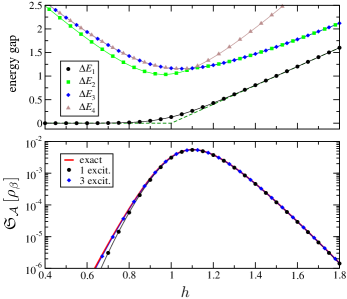
In the bottom panel of Fig. 8 we observe that, keeping only the ground and the first excited level in the computation of the energy variance (3), already gives an excellent approximation to the exact value of $\mathfrak{S}_{\cal AB}[\rho_{\beta}]$. Therefore the above situation effectively applies at large $\beta$ values. In the presence of a symmetry breaking mechanism, one would find a situation analogous to the LZ scheme: the presence of a maximum in proximity of $h_{c}$ would not be guaranteed, and a local minimum may appear (according to the values of $L$ and $\beta$).

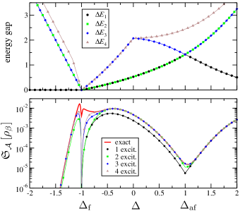
Let us now consider the XXZ-Heisenberg chain (10). Analogously as above, the upper panel of Fig. 9 displays the first energy levels in the full Hilbert space (we do not break the symmetry associated to the conservation of the global magnetization along the $z$ axis). For $\Delta<\Delta_{\rm f}$, the ground state is fully polarized along $z$, and presents a double degeneracy at any length. At $\Delta=\Delta_{\rm af}$ we see a cusp in the ground-state energy gap that is due to a level crossing (this feature persists at larger sizes $L$). This scenario characterizes the contribution to the heat capacity coming only by the ground state and the first excited state (black line in the bottom panel). In particular we see that, in this approximation, $\mathfrak{S}_{\cal AB}[\rho_{\beta}]$ is zero for $\Delta<\Delta_{\rm f}$, while it becomes finite at $\Delta>\Delta_{\rm f}$. On the other side, the $\Delta_{\rm af}$ is signaled by a cusp, which displays a minimum, and which raises as a consequence of the cusp in the ground-state energy gap.

Contrary to the Ising model, if also other excited levels are taken into account, non-negligible corrections to the energy variance appear (see the bottom panel of Fig. 9). In particular we note the emergence of a minimum around $\Delta_{\rm f}$, due to the fact that $\mathfrak{S}_{\cal AB}[\rho_{\beta}]$ becomes finite also for $J_{z}<\Delta_{\rm f}$. The corner point at $\Delta_{\rm af}$ is smeared into a local minimum with a continuous derivative. The positions of the two minima are influenced by finite-size and finite-temperature effects.

Figure 9: Same quantities and parameters as in Fig. 8, but for the XXZ chain in the full many-body Hilbert space of $L$ spins.

References

- (1) F. Giazotto, T. T. Heikkilä, A. Luukanen, A. M. Savin, and J. P. Pekola, Rev. Mod. Phys. 78, 217 (2006).
- (2) H. Cramér, Mathematical Methods of Statistics (Princeton University, Princeton, NJ, 1946).
- (3) M. G. A. Paris, and J. Řeháček, Quantum State Estimation (Lecture Notes in Physics vol. 649, Springer, 2004).
- (4) M. G. A. Paris, Int. J. Quant. Inf. 7,125 (2009).
- (5) P. Zanardi, P. Giorda, and M. Cozzini, Phys. Rev. Lett. 99, 100603 (2007).
- (6) P. Zanardi, M. G. A. Paris, and L. Campos Venuti, Phys. Rev. A 78, 042105 (2008).
- (7) Y. Gao and Y. Bando, Nature 415, 599 (2002).
- (8) D. M. Weld, P. Medley, H. Miyake, D. Hucul, D. E. Pritchard, and W. Ketterle, Phys. Rev. Lett. 103, 245301 (2009).
- (9) P. Neumann, I. Jakobi, F. Dolde, C. Burk, R. Reuter, G. Waldherr, J. Honert, T. Wolf, A. Brunner, and J. H. Shim, Nano Lett. 13, 2738 (2013).
- (10) G. Kucsko, P. C. Maurer, N. Y. Yao, M. Kubo, H. J. Noh, P. K. Lo, H. Park, and M. D. Lukin, Nature 500, 54 (2013).
- (11) F. Haupt, A. Imamoglu, and M. Kroner, Phys. Rev. Appl. 2, 024001 (2014).
- (12) F. Seilmeier, M. Hauck, E. Schubert, G. J. Schinner, S. E. Beavan, and A. Högele, Phys. Rev. Appl. 2, 024002 (2014).
- (13) K. Huang, Statistical Mechanics, (2nd edition, Wiley, New York, 1987).
- (14) T. L. Hill, Thermodynamics of Small Systems, (Dover, New York, 1994).
- (15) T. L. Hill, Nano Lett. 1, 273 (2001).
- (16) J. Gemmer, M. Michel, and G. Mahler, Quantum Thermodynamics, Lecture Notes in Physics, vol. 657 (Springer, Berlin, Heidelberg, New York, 2004).
- (17) A. E. Allahverdyan and Th. M. Nieuwenhuizen, Phys. Rev. Lett. 85, 1799 (2000).
- (18) A. E. Allahverdyan and Th. M. Nieuwenhuizen, Phys. Rev. B 66, 115309 (2002).
- (19) Th. M. Nieuwenhuizen and A. E. Allahverdyan, Phys. Rev. E 66, 036102 (2002).
- (20) S. Hilt and E. Lutz, Phys. Rev. A 79, 010101(R) (2009).
- (21) N. S. Williams, K. Le Hur, and A. N. Jordan, J. Phys. A: Math. Theor. 44, 385003 (2011).
- (22) M. Horodecki and J. Oppenheim, Nat. Commun. 4, 2059 (2013).
- (23) M. Brunelli, S. Olivares, and M. G. A. Paris, Phys. Rev. A 84, 032105 (2011).
- (24) M. Brunelli, S. Olivares, M. Paternostro, and M. G. A. Paris, Phys. Rev. A 86, 012125 (2012).
- (25) U. Marzolino and D. Braun, Phys. Rev. A 88, 063609 (2013); ibid. 91, 039902(E) (2015).
- (26) L. A. Correa, M. Mehboudi, G. Adesso, and A. Sanpera, Phys. Rev. Lett. 114, 220405 (2015).
- (27) G. Salvatori, A. Mandarino, and M. G. A. Paris, Phys. Rev. A 90, 022111 (2014).
- (28) M. Mehboudi, M. Moreno-Cardoner, G. De Chiara, and A. Sanpera, New J. Phys. 17, 055020 (2015).
- (29) M. Hartmann, G. Mahler, and O. Hess, Phys. Rev. Lett. 93, 080402 (2004).
- (30) M. Hartmann, G. Mahler, and O. Hess, Phys. Rev. E 70, 066148 (2004).
- (31) M. Hartmann and G. Mahler, Europhys. Lett. 70, 579 (2005).
- (32) A. García-Saez, A. Ferraro, and A. Acín, Phys.Rev. A 79, 052340 (2009).
- (33) A. Ferraro, A. García-Saez, and A. Acín, Europhys. Lett. 98, 10009 (2012).
- (34) M. Kliesch, C. Gogolin, M. J. Kastoryano, A. Riera, and J. Eisert, Phys. Rev. X 4, 031019 (2014).
- (35) V. Giovannetti, S. Lloyd, and L. Maccone, Nature Photon. 5, 222 (2011).
- (36) A. Peres, Phys. Rev. A 30, 1610 (1984).
- (37) R. Jozsa, J. Mod. Opt. 41, 2315 (1994).
- (38) A. Uhlmann, Rep. Math. Phys. 9, 273 (1976).
- (39) S. L. Braunstein and C. M. Caves, Phys. Rev. Lett. 72, 3439 (1994).
- (40) S. Sachdev, Quantum Phase Transitions (Cambridge University Press, Cambridge, England, 1999).
- (41) P. Zanardi, L. Campos Venuti, and P. Giorda, Phys. Rev. A. 76, 062318 (2007).
- (42) C. Zener, Proc. R. Soc. A 137, 696 (1932).
- (43) T. M. Stace, Phys. Rev. A 82, 011611(R) (2010).
- (44) M. Jarzyna and M. Zwierz, Phys. Rev. A 92, 032112 (2015).
- (45) M. Campisi, P. Hänggi, and P. Talkner, Rev. Mod. Phys. 83, 771 (2011).
-
(46)
R. Bhatia, Matrix Analysis (Springer, New York, 1997).