aainstitutetext: Fakultät für Physik, Universität Wien, Boltzmanngasse 5, 1090 Vienna, Austriabbinstitutetext: Erwin Schrödinger International Institute for Mathematical Physics, University of Vienna, Boltzmanngasse 9, A-1090 Vienna, Austria

Bottom and Charm Mass Determinations with a Convergence Test

Bahman Dehnadi a,b    André H. Hoang a    and Vicent Mateu bahman.dehnadi@univie.ac.at andre.hoang@univie.ac.at vicent.mateu@univie.ac.at
Abstract

We present new determinations of the MS¯¯MS\overline{\rm MS} charm quark mass using relativistic QCD sum rules at 𝒪(αs3)𝒪superscriptsubscript𝛼𝑠3{\cal O}(\alpha_{s}^{3}) from the moments of the vector and the pseudoscalar current correlators. We use available experimental measurements from e+esuperscript𝑒superscript𝑒e^{+}\,e^{-} collisions and lattice simulation results, respectively. Our analysis of the theoretical uncertainties is based on different implementations of the perturbative series and on independent variations of the renormalization scales for the mass and the strong coupling. Taking into account the resulting set of series to estimate perturbative uncertainties is crucial, since some ways to treat the perturbative expansion can exhibit extraordinarily small scale dependence when the two scales are set equal. As an additional refinement, we address the issue that double scale variation could overestimate the perturbative uncertainties. We supplement the analysis with a test that quantifies the convergence rate of each perturbative series by a single number. We find that this convergence test allows to determine an overall and average convergence rate that is characteristic for the series expansions of each moment, and to discard those series for which the convergence rate is significantly worse. We obtain m¯c(m¯c)= 1.288±0.020subscript¯𝑚𝑐subscript¯𝑚𝑐plus-or-minus1.2880.020\overline{m}_{c}(\overline{m}_{c})=\,1.288\,\pm 0.020\,GeV from the vector correlator. The method is also applied to the extraction of the MS¯¯MS\overline{\rm MS} bottom quark mass from the vector correlator. We compute the experimental moments including a modeling uncertainty associated to the continuum region where no data is available. We obtain m¯b(m¯b)= 4.176±0.023subscript¯𝑚𝑏subscript¯𝑚𝑏plus-or-minus4.1760.023\overline{m}_{b}(\overline{m}_{b})=\,4.176\,\pm 0.023\,GeV.

preprint: UWThPh-2015-09, LPN15-024

1 Introduction

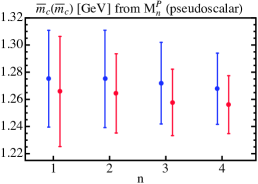
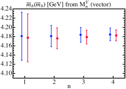
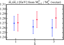
Precise and reliable determinations of the charm and bottom quark masses are an important input for a number of theoretical predictions, such as Higgs branching ratios to charm and bottom quarks or for the corresponding Yukawa couplings Heinemeyer:2013tqa ; Petrov:2015jea . They also affect the theoretical predictions of radiative and inclusive B decays, as well as rare kaon decays. For example, the inclusive semileptonic decay rate of B mesons depends on the fifth power of the bottom quark mass. These weak decays provide crucial methods to determine elements of the CKM matrix, which in turn are important for testing the validity of the Standard Model, as well as for indirect searches of new physics. In this context, having a reliable estimate of uncertainties for the quark masses is as important as knowing their precise values Antonelli:2009ws . Due to confinement quark masses are not physical observables. Rather, they are scheme-dependent parameters of the QCD Lagrangian which have to be determined from quantities that strongly depend on them.

One of the most precise tools to determine the charm and bottom quark masses is the QCD sum rule method, where weighted averages of the normalized cross section Re+eqq¯+Xsubscript𝑅superscript𝑒superscript𝑒𝑞¯𝑞𝑋R_{e^{+}e^{-}\to\,q\bar{q}\,+X}, with q=c,b𝑞𝑐𝑏q=c,b,

MnV=dssn+1Re+eqq¯+X(s),Re+eqq¯+X(s)=σe+eqq¯+X(s)σe+eμ+μ(s),formulae-sequencesuperscriptsubscript𝑀𝑛𝑉d𝑠superscript𝑠𝑛1subscript𝑅superscript𝑒superscript𝑒𝑞¯𝑞𝑋𝑠subscript𝑅superscript𝑒superscript𝑒𝑞¯𝑞𝑋𝑠subscript𝜎superscript𝑒superscript𝑒𝑞¯𝑞𝑋𝑠subscript𝜎superscript𝑒superscript𝑒superscript𝜇superscript𝜇𝑠\displaystyle M_{n}^{V}=\!\int\!\dfrac{{\rm d}s}{s^{n+1}}R_{e^{+}e^{-}\to\,q\bar{q}\,+X}(s)\,,\qquad R_{e^{+}e^{-}\to\,q\bar{q}\,+X}(s)=\dfrac{\sigma_{e^{+}e^{-}\to\,q\bar{q}\,+X}(s)}{\sigma_{e^{+}e^{-}\to\,\mu^{+}\mu^{-}}(s)}\,, (1)

can be related to moments of the quark vector current correlator ΠVsubscriptΠ𝑉\Pi_{V} Shifman:1978bx ; Shifman:1978by :

MnV,th=12π2Qq2n!dndsnΠV(s)|s=0,jμ(x)=q¯(x)γμq(x),formulae-sequencesuperscriptsubscript𝑀𝑛𝑉thevaluated-at12superscript𝜋2superscriptsubscript𝑄𝑞2𝑛superscriptd𝑛dsuperscript𝑠𝑛subscriptΠ𝑉𝑠𝑠0superscript𝑗𝜇𝑥¯𝑞𝑥superscript𝛾𝜇𝑞𝑥\displaystyle M_{n}^{V,\,\rm th}=\dfrac{12\pi^{2}Q_{q}^{2}}{n!}\,\dfrac{{\rm d}^{n}}{{\rm d}s^{n}}\Pi_{V}(s)\Big{|}_{s=0}\,,\quad\,j^{\mu}(x)=\bar{q}(x)\gamma^{\mu}q(x)\,,
(gμνsqμqν)ΠV(s)=idxeiqx 0|Tjμ(x)jν(0)|0.subscript𝑔𝜇𝜈𝑠subscript𝑞𝜇subscript𝑞𝜈subscriptΠ𝑉𝑠𝑖differential-d𝑥superscript𝑒𝑖𝑞𝑥quantum-operator-product 0𝑇subscript𝑗𝜇𝑥subscript𝑗𝜈00\displaystyle\big{(}g_{\mu\nu}\,s-q_{\mu}q_{\nu}\big{)}\Pi_{V}(s)=-\,i\!\int\!\mathrm{d}x\,e^{iqx}\left\langle\,0\left|T\,j_{\mu}(x)j_{\nu}(0)\right|0\,\right\rangle. (2)

Here Qqsubscript𝑄𝑞Q_{q} is the quark electric charge and s=q2𝑠superscript𝑞2\sqrt{s}=\sqrt{q^{2}} is the e+esuperscript𝑒superscript𝑒e^{+}e^{-} center-of-mass energy. Given that the integration over the experimental R𝑅R-ratio extends from the quark pair threshold up to infinity but experimental measurements only exist for energies up to around 111111 GeV, one relies on using theory input for energies above that scale (which we call the “continuum” region). For the charm moments, the combination of all available measurements is actually sufficient to render the experimental moments essentially independent of uncertainties one may assign to the theory input for the continuum region Dehnadi:2011gc . For the bottom moments, the dependence on the continuum theory input is very large, and the dependence of the low-n𝑛n experimental moments on unavoidable assumptions about the continuum uncertainty can be the most important component of the error budget, see e.g. Corcella:2002uu . In fact, the use of the first moment M1Vsuperscriptsubscript𝑀1𝑉M_{1}^{V} to determine the bottom mass appears to be excluded until more experimental data becomes available for higher energies.

Alternatively one can also consider moments of the pseudoscalar current correlator to extract the heavy quark masses. Experimental information on the pseudoscalar correlator ΠPsubscriptΠ𝑃\Pi_{P} is not available in a form useful for quark mass determinations, but for the charm quark very precise lattice calculations have become available recently Allison:2008xk . For the pseudoscalar correlator it turns out that the first two Taylor coefficients in the small-q2superscript𝑞2q^{2} expansion need to be regularized and defined in a given scheme, and that the third term (which we will denote by M0Psuperscriptsubscript𝑀0𝑃M_{0}^{P}) is hardly sensitive to mqsubscript𝑚𝑞m_{q}. We adopt the definitions

ΠP(s)=idxeiqx 0|TjP(x)jP(0)|0,jP(x)=2mqiq¯(x)γ5q(x),formulae-sequencesubscriptΠ𝑃𝑠𝑖differential-d𝑥superscript𝑒𝑖𝑞𝑥quantum-operator-product 0𝑇subscript𝑗𝑃𝑥subscript𝑗𝑃00subscript𝑗𝑃𝑥2subscript𝑚𝑞𝑖¯𝑞𝑥subscript𝛾5𝑞𝑥\displaystyle\Pi_{P}(s)=i\!\int\!\mathrm{d}x\,e^{iqx}\left\langle\,0\left|T\,j_{P}(x)j_{P}(0)\right|0\,\right\rangle,\quad j_{P}(x)=2\,m_{q}\,i\,\bar{q}(x)\gamma_{5}q(x)\,, (3)
MnP,th=12π2Qq2n!dndsnP(s)|s=0,P(s)=ΠP(s)ΠP(0)ΠP(0)ss2,formulae-sequencesuperscriptsubscript𝑀𝑛𝑃thevaluated-at12superscript𝜋2superscriptsubscript𝑄𝑞2𝑛superscriptd𝑛dsuperscript𝑠𝑛𝑃𝑠𝑠0𝑃𝑠subscriptΠ𝑃𝑠subscriptΠ𝑃0subscriptsuperscriptΠ𝑃0𝑠superscript𝑠2\displaystyle M_{n}^{P,\,\rm th}=\dfrac{12\pi^{2}Q_{q}^{2}}{n!}\,\dfrac{{\rm d}^{n}}{{\rm d}s^{n}}P(s)\Big{|}_{s=0}\,,\qquad P(s)=\dfrac{\Pi_{P}(s)-\Pi_{P}(0)-\Pi^{\prime}_{P}(0)\,s}{s^{2}}\,,

where the explicit mass factor in the definition of the pseudoscalar current ensures it is renormalization-scheme independent.

For small values of n𝑛n such that mq/nΛQCDgreater-than-or-equivalent-tosubscript𝑚𝑞𝑛subscriptΛQCDm_{q}/n\gtrsim\Lambda_{{\rm QCD}}, the theoretical moments for the vector and pseudoscalar correlators can be computed in the framework of the OPE, i.e. as an expansion in vacuum matrix elements involving operators of increasing dimension Shifman:1978bx ; Shifman:1978by . The leading matrix element corresponds to the perturbative QCD computations, which greatly dominates the series. Nonperturbative corrections are parametrized by vacuum condensates, and we find that even the leading correction, given by the gluon condensate, has a very small effect for low n𝑛n, particularly so for the bottom correlator. For moments at low values of n𝑛n, it is mandatory to employ a short-distance mass scheme such as MS¯¯MS\overline{\rm MS} Kuhn:2001dm , which renders the quark mass m¯q(μm)subscript¯𝑚𝑞subscript𝜇𝑚\overline{m}_{q}(\mu_{m}) dependent on its renormalization scale μmsubscript𝜇𝑚\mu_{m}, similar to the strong coupling αs(μα)subscript𝛼𝑠subscript𝜇𝛼\alpha_{s}(\mu_{\alpha}), which depends on μαsubscript𝜇𝛼\mu_{\alpha}. This method of determining the heavy quark masses with high precision is frequently called relativistic charmonium/bottomonium sum rules.

For the perturbative term, the exact analytic expressions for the ΠΠ\Pi functions are known at 𝒪(αs0)𝒪superscriptsubscript𝛼𝑠0{\mathcal{O}}(\alpha_{s}^{0}) and 𝒪(αs)𝒪subscript𝛼𝑠{\mathcal{O}}(\alpha_{s}), Kallen:1955fb . Therefore any moment can be obtained simply by Taylor expanding around q2=0superscript𝑞20q^{2}=0. At 𝒪(αs2)𝒪superscriptsubscript𝛼𝑠2{\mathcal{O}}(\alpha_{s}^{2}) moments are known to up to n=30𝑛30n=30 Chetyrkin:1995ii ; Chetyrkin:1996cf ; Boughezal:2006uu ; Czakon:2007qi ; Maier:2007yn . At 𝒪(αs3)𝒪superscriptsubscript𝛼𝑠3{\mathcal{O}}(\alpha_{s}^{3}) they are known analytically for n=1𝑛1n=1 Chetyrkin:2006xg ; Boughezal:2006px ; Sturm:2008eb , n=2𝑛2n=2 and n=3𝑛3n=3 (and even n=4𝑛4n=4 for the pseudoscalar correlator) Maier:2008he ; Maier:2009fz . Higher moments at 𝒪(αs3)𝒪superscriptsubscript𝛼𝑠3{\cal O}(\alpha_{s}^{3}) have been determined by a semi-analytical procedure Hoang:2008qy ; Kiyo:2009gb ; Greynat:2010kx ; Greynat:2011zp . The Wilson coefficient of the gluon condensate contribution is known to 𝒪(αs)𝒪subscript𝛼𝑠{\mathcal{O}}(\alpha_{s}) Broadhurst:1994qj .

The most recent determinations of the MS¯¯MS\overline{\rm MS} charm mass from charmonium sum rules for the vector correlator Dehnadi:2011gc ; Bodenstein:2011ma ; Chetyrkin:2009fv obtain very accurate results, but differ in the way they estimate theoretical uncertainties, and also in the computation of the moments from experimental data. Concerning the estimate of the perturbative uncertainties, Ref. Dehnadi:2011gc obtained 191919 MeV compared to 111 and 222 MeV obtained in Refs. Bodenstein:2011ma and Chetyrkin:2009fv , respectively. The discrepancy arises from two differences. First, in Refs. Bodenstein:2011ma ; Chetyrkin:2009fv the renormalization scales μmsubscript𝜇𝑚\mu_{m}, and μαsubscript𝜇𝛼\mu_{\alpha} were set equal, while in Ref. Dehnadi:2011gc it was argued that they should be varied independently. Second, in Refs. Bodenstein:2011ma ; Chetyrkin:2009fv the lowest renormalization scale was chosen to be 222 GeV, while in Ref. Dehnadi:2011gc variations down to the charm mass value were considered. For the case of the pseudoscalar moments, the HPQCD collaboration has made a number of very accurate predictions for charm and bottom masses Allison:2008xk ; McNeile:2010ji ; Chakraborty:2014aca ; Colquhoun:2014ica , the last of which has the smallest uncertainty claimed so far for the charm mass. In all these analyses the renormalization scales μmsubscript𝜇𝑚\mu_{m}, and μαsubscript𝜇𝛼\mu_{\alpha} are set equal when estimating the truncation uncertainty. A detailed discussion on the estimates of theoretical and experimental uncertainties can be found in Secs. 3 and 10 of this article (see also Ref. Dehnadi:2011gc ).

Similarly, bottomonium sum rules have been used to determine the bottom mass from low-n𝑛n moments. To the best of our knowledge, the most recent and precise determinations are from Refs. Bodenstein:2012 ; Chetyrkin:2009fv . These two analyses estimate their perturbative uncertainties in the same way as the corresponding charm mass extractions from the same collaborations Bodenstein:2011ma ; Chetyrkin:2009fv . Furthermore, when it comes to compute the experimental moments, they use theoretical input at 𝒪(αs3)𝒪superscriptsubscript𝛼𝑠3\mathcal{O}(\alpha_{s}^{3}) with perturbative uncertainties to model the high-energy region (continuum region) of the spectrum. As we discuss in this work, similar caveats as for their charm analyses can be argued to also affect their bottom quark results.

In this work we revisit the charmonium sum rules for the vector correlator, refining our perturbative error estimate from Ref. Dehnadi:2011gc by incorporating a convergence test. The convergence test addresses the issue that the independent variation of μmsubscript𝜇𝑚\mu_{m} and μαsubscript𝜇𝛼\mu_{\alpha} together with the relatively large value of the αssubscript𝛼𝑠\alpha_{s} close to the charm mass scale, might lead to an overestimate of the perturbative uncertainty. The convergence test allows to quantify the convergence property of each perturbative series with a single parameter and to discard series for which the convergence is substantially worse then for the rest of the series. We show that this procedure is meaningful, since the complete set of series for the moments shows a strongly peaked distribution in these convergence values, which allows to define an overall convergence for the set of perturbative series. This leads to a reduction of the perturbative uncertainty from 191919 to 141414 MeV, and the corresponding result for the MS¯¯MS\overline{\rm MS} charm mass supersedes the main result given in Ref. Dehnadi:2011gc . We also apply this improved method of estimating theory uncertainties to obtain a new charm mass determination from the pseudoscalar correlator, and to extract the bottom mass from the vector correlator. For the latter, we compute the bottom experimental moments by combining contributions from narrow resonances, experimental data taken in the continuum, and a theoretical model for the continuum region. We carefully study the assignment of adequate uncertainties to this last contribution, to make sure that the the model dependence is reduced to an acceptable level.

This paper is organized as follows: In Sec. 2 we summarize the theoretical framework introduced in Dehnadi:2011gc , and adapt it to cover the case of the pseudoscalar moments. We also introduce the ratios of moments, also used before in Ref. Kuhn:2001dm , and the perturbative expansions associated to them. Sec. 3 contains a brief summary of the results obtained in Dehnadi:2011gc , and the discussion is extended to the case of the pseudoscalar correlator and the bottom mass. In Sec. 4 we introduce the convergence test, and discuss how it allows to identify and discard series with a bad convergence. Sec. 5 contains a discussion on the lattice simulation results we use for our analysis. In Sec. 6 we present our computation of the experimental moments for the bottom correlator. The results are compared to previous determinations in Sec. 7. The computation of the ratio of experimental moments is presented in Sec. 8. Our final results for the quark masses are given in Sec. 9. The results are compared to previous charm and bottom mass analyses in Sec. 10. We present our conclusions in Sec. 11. In Appendix A the numerical values of the perturbative coefficients that enter into our analysis and are not yet provided by Ref. Dehnadi:2011gc are collected for the convenience of the reader.

2 Theoretical Input

2.1 Perturbative Contribution

The moments of the vector and pseudoscalar current correlators are defined in Eqs. (1) and (3), respectively. In the OPE framework they are dominated by the perturbative contribution (that is, a partonic computation), which exhibits a nonlinear dependence on the mass. Within perturbation theory one can decide to manipulate the series expansion to get a more linear dependence on the mass. Conceptually there is no preference. As advocated in our previous analyses Dehnadi:2011gc , one might consider various versions of the expansion to reliably estimate the perturbative uncertainties. Four types of expansion were suggested in Ref. Dehnadi:2011gc , which we briefly review below.


(a) Standard fixed-order expansion

We write the perturbative vacuum polarization function as

Π^X(s,nf,αs(nf)(μα),m¯q(μm),μα,μm)=112π2Qq2n=0snM^nX,subscript^Π𝑋𝑠subscript𝑛𝑓superscriptsubscript𝛼𝑠subscript𝑛𝑓subscript𝜇𝛼subscript¯𝑚𝑞subscript𝜇𝑚subscript𝜇𝛼subscript𝜇𝑚112superscript𝜋2superscriptsubscript𝑄𝑞2superscriptsubscript𝑛0superscript𝑠𝑛subscriptsuperscript^𝑀𝑋𝑛\displaystyle\widehat{\Pi}_{X}(s,n_{f},\alpha_{s}^{(n_{f})}(\mu_{\alpha}),\overline{m}_{q}(\mu_{m}),\mu_{\alpha},\mu_{m})\,=\,\dfrac{1}{12\pi^{2}Q_{q}^{2}}\sum_{n=0}^{\infty}s^{n}\hat{M}^{X}_{n}\,, (4)

where X=V,P𝑋𝑉𝑃X=V,P for vector and pseudoscalar currents, respectively. Note that for notation reasons, in Eqs. (4, 8, 10, 11) we use ΠP(q2)=P(q2)subscriptΠ𝑃superscript𝑞2𝑃superscript𝑞2\Pi_{P}(q^{2})=P(q^{2}), where P𝑃P is the twice-subtracted pseudoscalar correlator defined in Eq. (3). Here Qqsubscript𝑄𝑞Q_{q} is the quark electric charge with q=c,b𝑞𝑐𝑏q=c,b, and nf=4,5subscript𝑛𝑓45n_{f}=4,5 for charm and bottom, respectively. In full generality, the perturbative moments M^nsubscript^𝑀𝑛\hat{M}_{n} can be expressed as the following sum:

M^nXsubscriptsuperscript^𝑀𝑋𝑛\displaystyle\hat{M}^{X}_{n} =\displaystyle= 1[4m¯q 2(μm)]ni,a,b(αs(nf)(μα)π)i[CX(nf)]n,ia,blna(m¯q 2(μm)μm2)lnb(m¯q 2(μm)μα2).1superscriptdelimited-[]4subscriptsuperscript¯𝑚2𝑞subscript𝜇𝑚𝑛subscript𝑖𝑎𝑏superscriptsubscriptsuperscript𝛼subscript𝑛𝑓𝑠subscript𝜇𝛼𝜋𝑖subscriptsuperscriptdelimited-[]subscript𝐶𝑋subscript𝑛𝑓𝑎𝑏𝑛𝑖superscript𝑎subscriptsuperscript¯𝑚2𝑞subscript𝜇𝑚subscriptsuperscript𝜇2𝑚superscript𝑏subscriptsuperscript¯𝑚2𝑞subscript𝜇𝑚subscriptsuperscript𝜇2𝛼\displaystyle\frac{1}{[4\,\overline{m}^{\,2}_{q}(\mu_{m})]^{n}}\sum_{i,a,b}\bigg{(}\frac{\alpha^{(n_{f})}_{s}(\mu_{\alpha})}{\pi}\bigg{)}^{\!i}[C_{X}(n_{f})]^{a,b}_{n,i}\,\ln^{a}\!\bigg{(}\frac{\overline{m}^{\,2}_{q}(\mu_{m})}{\mu^{2}_{m}}\bigg{)}\!\ln^{b}\!\bigg{(}\frac{\overline{m}^{\,2}_{q}(\mu_{m})}{\mu^{2}_{\alpha}}\bigg{)}. (5)

This is the standard fixed-order expression for the perturbative moments. The numerical values for the [CV(nf=5)]n,ia,bsubscriptsuperscriptdelimited-[]subscript𝐶𝑉subscript𝑛𝑓5𝑎𝑏𝑛𝑖[C_{V}(n_{f}=5)]^{a,b}_{n,i} coefficients are given in Table 8 (for the vector current with nf=4subscript𝑛𝑓4n_{f}=4, these coefficients can be found in Table 1 of Ref. Dehnadi:2011gc ). Likewise, [CP(nf=4)]n,ia,bsubscriptsuperscriptdelimited-[]subscript𝐶𝑃subscript𝑛𝑓4𝑎𝑏𝑛𝑖[C_{P}(n_{f}=4)]^{a,b}_{n,i} are collected in a numerical form in Table 11.

The expression in Eq. (5) is the common way to write the perturbative series of the moments. However, as noted in Ref. Dehnadi:2011gc , the nonlinear dependence on m¯qsubscript¯𝑚𝑞\overline{m}_{q} of the standard fixed-order expansion has the disadvantage that for charm (bottom) quarks there are frequently no solutions for the mass in the sum rule mass determination, for moments higher than the first (second), for some set of values of the renormalization scales.


(b) Linearized expansion

One can linearize the the fixed-order form expansion of Eq. (5) with respect to the exponent of the quark mass pre-factor by taking the 2n2𝑛2n-th root. This choice is e.g. made in Ref. McNeile:2010ji , and in general one can write:

(M^nX)1/2n=12m¯q(μm)i,a,b(αs(nf)(μα)π)i[C¯X(nf)]n,ia,blna(m¯q 2(μm)μm2)lnb(m¯q 2(μm)μα2).superscriptsubscriptsuperscript^𝑀𝑋𝑛12𝑛12subscript¯𝑚𝑞subscript𝜇𝑚subscript𝑖𝑎𝑏superscriptsubscriptsuperscript𝛼subscript𝑛𝑓𝑠subscript𝜇𝛼𝜋𝑖superscriptsubscriptdelimited-[]subscript¯𝐶𝑋subscript𝑛𝑓𝑛𝑖𝑎𝑏superscript𝑎subscriptsuperscript¯𝑚2𝑞subscript𝜇𝑚subscriptsuperscript𝜇2𝑚superscript𝑏subscriptsuperscript¯𝑚2𝑞subscript𝜇𝑚subscriptsuperscript𝜇2𝛼\displaystyle\Big{(}\hat{M}^{X}_{n}\Big{)}^{\!1/2n}=\frac{1}{2\,\overline{m}_{q}(\mu_{m})}\,\sum_{i,a,b}\bigg{(}\frac{\alpha^{(n_{f})}_{s}(\mu_{\alpha})}{\pi}\bigg{)}^{\!i}[\bar{C}_{X}(n_{f})]_{n,i}^{a,b}\,\ln^{a}\!\bigg{(}\frac{\overline{m}^{\,2}_{q}(\mu_{m})}{\mu^{2}_{m}}\bigg{)}\!\ln^{b}\!\bigg{(}\frac{\overline{m}^{\,2}_{q}(\mu_{m})}{\mu^{2}_{\alpha}}\bigg{)}. (6)

The coefficients [C¯V(nf=5)]n,ia,bsuperscriptsubscriptdelimited-[]subscript¯𝐶𝑉subscript𝑛𝑓5𝑛𝑖𝑎𝑏[\bar{C}_{V}(n_{f}=5)]_{n,i}^{a,b} and [C¯P(nf=4)]n,ia,bsuperscriptsubscriptdelimited-[]subscript¯𝐶𝑃subscript𝑛𝑓4𝑛𝑖𝑎𝑏[\bar{C}_{P}(n_{f}=4)]_{n,i}^{a,b} are given in Tables 9 and 12, respectively (for nf=4subscript𝑛𝑓4n_{f}=4 the coefficients for the vector current can be found in Table 2 of Ref. Dehnadi:2011gc ). Even though relation (6) still exhibits some nonlinear dependence on m¯qsubscript¯𝑚𝑞{\overline{m}}_{q} through perturbative logarithms, we find that it always has a solution for the quark mass.


(c) Iterative linearized expansion

For the expansion methods (a) and (b) shown in Eqs. (5) and (6), one solves for the quark masses m¯c,b(μm)subscript¯𝑚𝑐𝑏subscript𝜇𝑚\overline{m}_{c,b}(\mu_{m}) numerically keeping the exact mass dependence on the theory side of the equation. Alternatively, one can solve for m¯c,b(μm)subscript¯𝑚𝑐𝑏subscript𝜇𝑚\overline{m}_{c,b}(\mu_{m}) iteratively order by order, which is perturbatively equivalent to the exact numerical solution, but gives different numerical results. The method consists of inserting the lower order values for m¯c,b(μm)subscript¯𝑚𝑐𝑏subscript𝜇𝑚\overline{m}_{c,b}(\mu_{m}) in the higher order perturbative coefficients, and re-expanding consistently. This method has been explained in detail in Sec. 2.1(c) of Ref. Dehnadi:2011gc , and we only quote the final results here:

m¯q(μm)subscript¯𝑚𝑞subscript𝜇𝑚\displaystyle{\overline{m}}_{q}(\mu_{m}) =m¯q(0)i,a,b(αs(nf)(μα)π)i[C~X(nf)]n,ia,blna(m¯q(0) 2μm2)lnb(m¯q(0) 2μα2),absentsuperscriptsubscript¯𝑚𝑞0subscript𝑖𝑎𝑏superscriptsubscriptsuperscript𝛼subscript𝑛𝑓𝑠subscript𝜇𝛼𝜋𝑖superscriptsubscriptdelimited-[]subscript~𝐶𝑋subscript𝑛𝑓𝑛𝑖𝑎𝑏superscript𝑎superscriptsubscript¯𝑚𝑞02subscriptsuperscript𝜇2𝑚superscript𝑏superscriptsubscript¯𝑚𝑞02subscriptsuperscript𝜇2𝛼\displaystyle=\,{\overline{m}}_{q}^{(0)}\sum_{i,a,b}\bigg{(}\frac{\alpha^{(n_{f})}_{s}(\mu_{\alpha})}{\pi}\bigg{)}^{\!i}[\tilde{C}_{X}(n_{f})]_{n,i}^{a,b}\,\ln^{a}\!\bigg{(}\frac{{\overline{m}}_{q}^{(0)\,2}}{\mu^{2}_{m}}\bigg{)}\!\ln^{b}\!\bigg{(}\frac{{\overline{m}}_{q}^{(0)\,2}}{\mu^{2}_{\alpha}}\bigg{)}, (7)
m¯q(0)(μm)superscriptsubscript¯𝑚𝑞0subscript𝜇𝑚\displaystyle\overline{m}_{q}^{(0)}(\mu_{m}) =12(MnX)1/2n[C~X(nf)]n,00,0,absent12superscriptsubscriptsuperscript𝑀𝑋𝑛12𝑛superscriptsubscriptdelimited-[]subscript~𝐶𝑋subscript𝑛𝑓𝑛000\displaystyle=\frac{1}{2\big{(}M^{X}_{n}\big{)}^{1/2n}}\,[\tilde{C}_{X}(n_{f})]_{n,0}^{0,0}\,,

where the numerical value of the coefficients [C~V(nf=5)]n,ia,bsuperscriptsubscriptdelimited-[]subscript~𝐶𝑉subscript𝑛𝑓5𝑛𝑖𝑎𝑏[\tilde{C}_{V}(n_{f}=5)]_{n,i}^{a,b} and [C~P(nf=4)]n,ia,bsuperscriptsubscriptdelimited-[]subscript~𝐶𝑃subscript𝑛𝑓4𝑛𝑖𝑎𝑏[\tilde{C}_{P}(n_{f}=4)]_{n,i}^{a,b} are collected in Tables 10 and 13, and the values for the vector current with nf=4subscript𝑛𝑓4n_{f}=4 can be found in Table 3 of Ref. Dehnadi:2011gc .

By construction, the iterative expansion always has a solution for the quark mass. Accordingly, potential biases on the numerical analysis related to any possible nonlinear dependence are eliminated.


(d) Contour-improved expansion

For the expansions (a), (b) and (c) the moments and the quark masses are computed for a fixed value of the renormalization scale μαsubscript𝜇𝛼\mu_{\alpha}. Using the analytic properties of the vacuum polarization function, one can rewrite the fixed-order moments as integrals in the complex plane. This opens the possibility of making μαsubscript𝜇𝛼\mu_{\alpha} dependent on the integration variable, in analogy to the contour-improved methods used for τ𝜏\tau-decays (see e.g. Refs. LeDiberder:1992te ; Pivovarov:1991rh ; Braaten:1991qm ; Narison:1988ni ; Braaten:1988ea ; Braaten:1988hc ). Therefore we define the contour-improved moments Hoang:2004xm as (see Fig. 1),

Refer to caption
Figure 1: One possible integration path in the complex s¯¯𝑠\bar{s}-plane for the computation of the contour-improved moments.
M^nX,𝒞superscriptsubscript^𝑀𝑛𝑋𝒞\displaystyle\hat{M}_{n}^{X,\mathcal{C}} =\displaystyle= 6πQq2i𝒞dssn+1Π^X(s,nf,αs(nf)(μαc(s,m¯q 2)),m¯q(μm),μαq(s,m¯q 2),μm),6𝜋superscriptsubscript𝑄𝑞2𝑖subscript𝒞d𝑠superscript𝑠𝑛1subscript^Π𝑋𝑠subscript𝑛𝑓superscriptsubscript𝛼𝑠subscript𝑛𝑓superscriptsubscript𝜇𝛼𝑐𝑠superscriptsubscript¯𝑚𝑞2subscript¯𝑚𝑞subscript𝜇𝑚superscriptsubscript𝜇𝛼𝑞𝑠superscriptsubscript¯𝑚𝑞2subscript𝜇𝑚\displaystyle\frac{6\pi Q_{q}^{2}}{i}\,\int_{\mathcal{C}}\,\frac{{\rm d}s}{s^{n+1}}\widehat{\Pi}_{X}(s,n_{f},\alpha_{s}^{(n_{f})}(\mu_{\alpha}^{c}(s,\overline{m}_{q}^{\,2})),\overline{m}_{q}(\mu_{m}),\mu_{\alpha}^{q}(s,\overline{m}_{q}^{\,2}),\mu_{m})\,, (8)

and we employ the following path-dependent μαcsuperscriptsubscript𝜇𝛼𝑐\mu_{\alpha}^{c}, first used in Ref. Hoang:2004xm

(μαq)2(s,m¯q 2)superscriptsuperscriptsubscript𝜇𝛼𝑞2𝑠superscriptsubscript¯𝑚𝑞2\displaystyle(\mu_{\alpha}^{q})^{2}(s,\overline{m}_{q}^{\,2}) =\displaystyle= μα2( 1s4m¯q 2(μm)).superscriptsubscript𝜇𝛼21𝑠4superscriptsubscript¯𝑚𝑞2subscript𝜇𝑚\displaystyle\mu_{\alpha}^{2}\,\bigg{(}\,1-\frac{s}{4\,\overline{m}_{q}^{\,2}(\mu_{m})}\,\bigg{)}\,. (9)

It weights in a different way the threshold versus the high energy parts of the spectrum. It was shown in Ref. Dehnadi:2011gc that the resulting moments M^nX,𝒞superscriptsubscript^𝑀𝑛𝑋𝒞\hat{M}_{n}^{X,\mathcal{C}} can be obtained analytically from the Taylor expansion around s=0𝑠0s=0 of the vacuum polarization function using an s𝑠s-dependent μαc(s,m¯q 2)superscriptsubscript𝜇𝛼𝑐𝑠superscriptsubscript¯𝑚𝑞2\mu_{\alpha}^{c}(s,\overline{m}_{q}^{\,2}):

Π^XMS¯(s,αs(nf)(μαc(s,m¯q 2)),m¯q(μm),μαc(s,m¯q 2),μm)superscriptsubscript^Π𝑋¯MS𝑠subscriptsuperscript𝛼subscript𝑛𝑓𝑠superscriptsubscript𝜇𝛼𝑐𝑠superscriptsubscript¯𝑚𝑞2subscript¯𝑚𝑞subscript𝜇𝑚superscriptsubscript𝜇𝛼𝑐𝑠superscriptsubscript¯𝑚𝑞2subscript𝜇𝑚\displaystyle\widehat{\Pi}_{X}^{\overline{\rm MS}}\Big{(}s,\alpha^{(n_{f})}_{s}(\mu_{\alpha}^{c}(s,\overline{m}_{q}^{\,2})),\overline{m}_{q}(\mu_{m}),\mu_{\alpha}^{c}(s,\overline{m}_{q}^{\,2}),\mu_{m}\Big{)} =\displaystyle= n=0snM^nX,𝒞.superscriptsubscript𝑛0superscript𝑠𝑛superscriptsubscript^𝑀𝑛𝑋𝒞\displaystyle\sum\limits_{n=0}^{\infty}\,s^{n}\,\hat{M}_{n}^{X,\mathcal{C}}\,. (10)

This trick works because αs(μαc(s,m¯q 2))subscript𝛼𝑠superscriptsubscript𝜇𝛼𝑐𝑠superscriptsubscript¯𝑚𝑞2\alpha_{s}(\mu_{\alpha}^{c}(s,\overline{m}_{q}^{\,2})) has the same cut as the fixed-order expression for Π^Xsubscript^Π𝑋\widehat{\Pi}_{X}. Other choices could spoil this property. Expanding the analytic expression for M^nX,𝒞superscriptsubscript^𝑀𝑛𝑋𝒞\hat{M}_{n}^{X,\mathcal{C}} on αssubscript𝛼𝑠\alpha_{s} at a given finite order, one recovers the fixed-order moments M^nXsuperscriptsubscript^𝑀𝑛𝑋\hat{M}_{n}^{X}. This shows that the dependence on the contour is only residual and represents an effect from higher order terms from beyond the order one employs for the calculation.

The contour-improved moments have a residual sensitivity to the value of the vacuum polarization function at zero momentum transfer.111This means that the dependence vanishes in the large-order limit. For the case of the vector correlator this value depends on the UV-subtraction scheme and corresponds to Π^(0)=M^0V^Π0superscriptsubscript^𝑀0𝑉\widehat{\Pi}(0)=\hat{M}_{0}^{V}. For the case of the pseudoscalar correlator, M^0Psuperscriptsubscript^𝑀0𝑃\hat{M}_{0}^{P} is scheme-independent, since P(q2)𝑃superscript𝑞2P(q^{2}) already includes two UV subtractions. However, one could as well define a three-times-subtracted pseudoscalar correlator of the form P¯(q2)=P(q2)P(0)¯𝑃superscript𝑞2𝑃superscript𝑞2𝑃0\overline{P}(q^{2})=P(q^{2})-P(0). Slightly abusing notation, we denote P¯¯𝑃\overline{P} as the “on-shell” scheme for P(q2)𝑃superscript𝑞2P(q^{2}), and the twice subtracted (original) definition as the MS¯¯MS\overline{\rm MS} scheme for P(q2)𝑃superscript𝑞2P(q^{2}). Using the OS scheme with Π^X(0)=0superscript^Π𝑋00\widehat{\Pi}^{X}(0)=0 for either vector or pseudoscalar correlator, we find that the first moment for the contour-improved expansion gives exactly the first fixed-order moment, M^1X,𝒞=M^1Xsuperscriptsubscript^𝑀1𝑋𝒞superscriptsubscript^𝑀1𝑋\hat{M}_{1}^{X,\mathcal{C}}=\hat{M}_{1}^{X}. Thus, in order to implement a non-trivial modification, and following Ref. Dehnadi:2011gc , we employ the MS¯¯MS\overline{\rm MS} scheme for Π^V(0)subscript^Π𝑉0\widehat{\Pi}_{V}(0) defined for μ=m¯q(m¯q)𝜇subscript¯𝑚𝑞subscript¯𝑚𝑞\mu={\overline{m}}_{q}({\overline{m}}_{q}), and the twice-subtracted expression for P(q2)𝑃superscript𝑞2P(q^{2}). Generically it can be written as

Π^XMS¯(0,nf)superscriptsubscript^Π𝑋¯MS0subscript𝑛𝑓\displaystyle\widehat{\Pi}_{X}^{\overline{\rm MS}}(0,n_{f}) =\displaystyle= i,a,b(αs(nf)(μα)π)i[CX(nf)]0,ia,blna(m¯q 2(μm)μm2)lnb(m¯q 2(μm)μα2).subscript𝑖𝑎𝑏superscriptsubscriptsuperscript𝛼subscript𝑛𝑓𝑠subscript𝜇𝛼𝜋𝑖subscriptsuperscriptdelimited-[]subscript𝐶𝑋subscript𝑛𝑓𝑎𝑏0𝑖superscript𝑎subscriptsuperscript¯𝑚2𝑞subscript𝜇𝑚subscriptsuperscript𝜇2𝑚superscript𝑏subscriptsuperscript¯𝑚2𝑞subscript𝜇𝑚subscriptsuperscript𝜇2𝛼\displaystyle\sum_{i,a,b}\bigg{(}\frac{\alpha^{(n_{f})}_{s}(\mu_{\alpha})}{\pi}\bigg{)}^{\!i}[C_{X}(n_{f})]^{a,b}_{0,i}\,\ln^{a}\!\bigg{(}\frac{\overline{m}^{\,2}_{q}(\mu_{m})}{\mu^{2}_{m}}\bigg{)}\!\ln^{b}\!\bigg{(}\frac{\overline{m}^{\,2}_{q}(\mu_{m})}{\mu^{2}_{\alpha}}\bigg{)}. (11)

The numerical values for the coefficients [CX]0,ia,bsubscriptsuperscriptdelimited-[]subscript𝐶𝑋𝑎𝑏0𝑖[C_{X}]^{a,b}_{0,i} are collected in Table 7 for the vector correlator with 555 flavors and the pseudoscalar correlator with 444 flavors. In Table 4 or Ref. Dehnadi:2011gc one finds the the numerical values of [CV(nf=4)]0,ia,bsubscriptsuperscriptdelimited-[]subscript𝐶𝑉subscript𝑛𝑓4𝑎𝑏0𝑖[C_{V}(n_{f}=4)]^{a,b}_{0,i}.

Refer to caption
Refer to caption
Refer to caption
Refer to caption
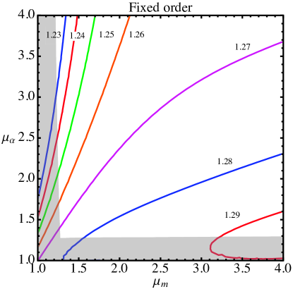
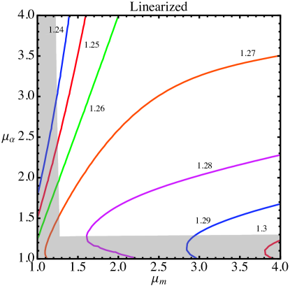
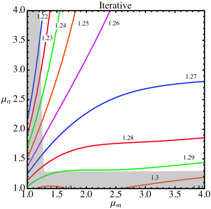
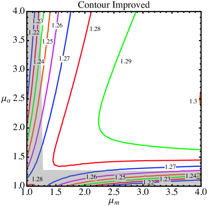
Figure 2: Contour plots for m¯c(m¯c)subscript¯𝑚𝑐subscript¯𝑚𝑐\overline{m}_{c}(\overline{m}_{c}) as obtained from the first moment of the pseudoscalar correlator M1Psuperscriptsubscript𝑀1𝑃M_{1}^{P}, as a function of μαsubscript𝜇𝛼\mu_{\alpha} and μmsubscript𝜇𝑚\mu_{m} at 𝒪(αs3)𝒪superscriptsubscript𝛼𝑠3{\mathcal{O}}(\alpha_{s}^{3}), for methods (a) – (d). The shaded areas represent regions with μm,μα<m¯c(m¯c)subscript𝜇𝑚subscript𝜇𝛼subscript¯𝑚𝑐subscript¯𝑚𝑐\mu_{m},\mu_{\alpha}<\overline{m}_{c}(\overline{m}_{c}), and are excluded of our analysis. For this plot we employ αs(mZ)=0.118subscript𝛼𝑠subscript𝑚𝑍0.118\alpha_{s}(m_{Z})=0.118.
Refer to caption
Refer to caption
Refer to caption
Refer to caption
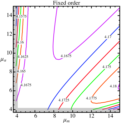
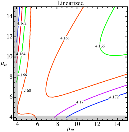
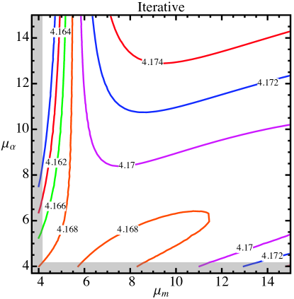
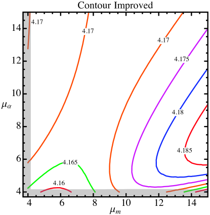
Figure 3: Contour plots for m¯b(m¯b)subscript¯𝑚𝑏subscript¯𝑚𝑏\overline{m}_{b}(\overline{m}_{b}) as obtained from the second moment of the vector correlator M2Vsuperscriptsubscript𝑀2𝑉M_{2}^{V} with nf=5subscript𝑛𝑓5n_{f}=5, as a function of μαsubscript𝜇𝛼\mu_{\alpha} and μmsubscript𝜇𝑚\mu_{m} at 𝒪(αs3)𝒪superscriptsubscript𝛼𝑠3{\mathcal{O}}(\alpha_{s}^{3}), for methods (a) – (d). The shaded areas represent regions with μm,μα<m¯b(m¯b)subscript𝜇𝑚subscript𝜇𝛼subscript¯𝑚𝑏subscript¯𝑚𝑏\mu_{m},\mu_{\alpha}<\overline{m}_{b}(\overline{m}_{b}), and are excluded of our analysis. For this plot we employ αs(mZ)=0.118subscript𝛼𝑠subscript𝑚𝑍0.118\alpha_{s}(m_{Z})=0.118.

2.2 Gluon Condensate Contribution

We estimate nonperturbative power corrections by including the gluon condensate contribution. The gluon condensate is a dimension-4 matrix element and gives the leading power correction in the OPE for the moments Novikov:1977dq ; Baikov:1993kc

MnXsubscriptsuperscript𝑀𝑋𝑛\displaystyle M^{X}_{n} =\displaystyle= M^nX+ΔMnX,G2+superscriptsubscript^𝑀𝑛𝑋Δsuperscriptsubscript𝑀𝑛𝑋delimited-⟨⟩superscript𝐺2\displaystyle\hat{M}_{n}^{X}+\Delta M_{n}^{X,\,\langle G^{2}\rangle}\,+\,\ldots (12)

Here the ellipses represent higher-order power corrections of the OPE involving condensates with dimensions bigger than 444. The Wilson coefficients of the gluon condensate corrections are known to 𝒪(αs)𝒪subscript𝛼𝑠\mathcal{O}(\alpha_{s}) accuracy Broadhurst:1994qj . Following Ref. Chetyrkin:2010ic , we express the Wilson coefficient of the gluon condensate in terms of the pole mass, since in this way the correction is numerically more stable for higher moments. However, as we did in Ref. Dehnadi:2011gc , we still write the pole mass in terms of the MS¯¯MS\overline{\mbox{MS}} quark mass at one loop. The resulting expression reads

ΔMnX,G2Δsuperscriptsubscript𝑀𝑛𝑋delimited-⟨⟩superscript𝐺2\displaystyle\Delta M_{n}^{X,\,\langle G^{2}\rangle} =\displaystyle= 1(4Mq2)n+2αsπG2RGI[[aX(nf)]n0+αs(nf)(μα)π[aX(nf)]n1],1superscript4superscriptsubscript𝑀𝑞2𝑛2subscriptdelimited-⟨⟩subscript𝛼𝑠𝜋superscript𝐺2RGIdelimited-[]subscriptsuperscriptdelimited-[]subscript𝑎𝑋subscript𝑛𝑓0𝑛subscriptsuperscript𝛼subscript𝑛𝑓𝑠subscript𝜇𝛼𝜋subscriptsuperscriptdelimited-[]subscript𝑎𝑋subscript𝑛𝑓1𝑛\displaystyle\dfrac{1}{(4M_{q}^{2})^{n+2}}\Big{\langle}\frac{\alpha_{s}}{\pi}G^{2}\Big{\rangle}_{\rm RGI}\left[[a_{X}(n_{f})]^{0}_{n}+\dfrac{\alpha^{(n_{f})}_{s}(\mu_{\alpha})}{\pi}\,[a_{X}(n_{f})]^{1}_{n}\right], (13)
Mqsubscript𝑀𝑞\displaystyle M_{q} =\displaystyle= m¯q(μm){1+αs(nf)(μα)π[43ln(m¯q 2(μm)μm2)]}.subscript¯𝑚𝑞subscript𝜇𝑚1subscriptsuperscript𝛼subscript𝑛𝑓𝑠subscript𝜇𝛼𝜋delimited-[]43subscriptsuperscript¯𝑚2𝑞subscript𝜇𝑚subscriptsuperscript𝜇2𝑚\displaystyle\overline{m}_{q}(\mu_{m})\left\{1+\dfrac{\alpha^{(n_{f})}_{s}(\mu_{\alpha})}{\pi}\left[\dfrac{4}{3}-\ln\left(\frac{\overline{m}^{\,2}_{q}(\mu_{m})}{\mu^{2}_{m}}\right)\right]\right\}.

We use the renormalization group invariant (RGI) scheme for the gluon condensate Narison:1983kn . The numerical value of the [aV(nf=5)]nasubscriptsuperscriptdelimited-[]subscript𝑎𝑉subscript𝑛𝑓5𝑎𝑛[a_{V}(n_{f}=5)]^{a}_{n} and [aP(nf=4)]nasubscriptsuperscriptdelimited-[]subscript𝑎𝑃subscript𝑛𝑓4𝑎𝑛[a_{P}(n_{f}=4)]^{a}_{n} coefficients are collected in Table 6. The values for [aV(nf=4)]nasubscriptsuperscriptdelimited-[]subscript𝑎𝑉subscript𝑛𝑓4𝑎𝑛[a_{V}(n_{f}=4)]^{a}_{n} can be found in Table 5 of Ref. Dehnadi:2011gc . For methods (b) and (c) one can obtain the gluon condensate contribution by performing simple algebra operations and re-expansions in αs(nf)superscriptsubscript𝛼𝑠subscript𝑛𝑓\alpha_{s}^{(n_{f})} and G2delimited-⟨⟩superscript𝐺2\langle G^{2}\rangle. For method (d) we employ Eqs. (12) and (13) as shown. For the RGI gluon condensate we adopt Ioffe:2005ym

αsπG2RGIsubscriptdelimited-⟨⟩subscript𝛼𝑠𝜋superscript𝐺2RGI\displaystyle\Big{\langle}\frac{\alpha_{s}}{\pi}G^{2}\Big{\rangle}_{\rm RGI} =\displaystyle= 0.006±0.012GeV4.plus-or-minus0.0060.012superscriptGeV4\displaystyle 0.006\pm 0.012\;\mathrm{GeV}^{4}\,. (14)

2.3 Ratios of Moments

An alternative set of observables which are also highly sensitive to the quark masses are the ratios of consecutive moments. To that end we define RnX(nf)Mn+1X(nf)/MnX(nf)superscriptsubscript𝑅𝑛𝑋subscript𝑛𝑓subscriptsuperscript𝑀𝑋𝑛1subscript𝑛𝑓subscriptsuperscript𝑀𝑋𝑛subscript𝑛𝑓R_{n}^{X}(n_{f})\equiv M^{X}_{n+1}(n_{f})/M^{X}_{n}(n_{f}). Such ratios are proportional to the inverse square of the quark mass for any value of n𝑛n. Their perturbative series can be expressed as an expansion in powers of αs(nf)superscriptsubscript𝛼𝑠subscript𝑛𝑓\alpha_{s}^{(n_{f})} analogous to Eq. (5), with the replacements [4m¯q 2(μm)]n4m¯q 2(μm)superscriptdelimited-[]4superscriptsubscript¯𝑚𝑞2subscript𝜇𝑚𝑛4superscriptsubscript¯𝑚𝑞2subscript𝜇𝑚[4\,\overline{m}_{q}^{\,2}(\mu_{m})]^{n}\to 4\,\overline{m}_{q}^{\,2}(\mu_{m}) and [CX(nf)]a,bi,j[RX(nf)]a,bi,jsuperscriptsubscriptdelimited-[]subscript𝐶𝑋subscript𝑛𝑓𝑎𝑏𝑖𝑗superscriptsubscriptdelimited-[]subscript𝑅𝑋subscript𝑛𝑓𝑎𝑏𝑖𝑗[C_{X}(n_{f})]_{a,b}^{i,j}\to[R_{X}(n_{f})]_{a,b}^{i,j}. Their computation is trivial, as one only needs to take the ratio of the two consecutive theoretical moments and re-expand as a series in αs(nf)superscriptsubscript𝛼𝑠subscript𝑛𝑓\alpha_{s}^{(n_{f})}. We call this the standard fixed-order expansion, analogous to the expansion (a) of Sec. 2.1. The numerical expressions for the [RX(nf)]a,bi,jsuperscriptsubscriptdelimited-[]subscript𝑅𝑋subscript𝑛𝑓𝑎𝑏𝑖𝑗[R_{X}(n_{f})]_{a,b}^{i,j} coefficients for the vector correlator with nf=4,5subscript𝑛𝑓45n_{f}=4,5 are given in Table 14, and for the pseudoscalar correlator with nf=4subscript𝑛𝑓4n_{f}=4 in Table 15. As for the regular moments, we find that the nonlinear dependence of RnXsuperscriptsubscript𝑅𝑛𝑋R_{n}^{X} on the quark mass sometimes causes that there is no numerical solution for m¯qsubscript¯𝑚𝑞\overline{m}_{q}.

By taking the square root of the ratio of two consecutive moments one gets a linear dependence on the inverse of the quark mass. The corresponding theoretical expression is obtained by re-expanding the perturbative expansion of RnX(nf)superscriptsubscript𝑅𝑛𝑋subscript𝑛𝑓\sqrt{R_{n}^{X}(n_{f})} as a series in powers of αs(nf)superscriptsubscript𝛼𝑠subscript𝑛𝑓\alpha_{s}^{(n_{f})}. Thus we obtain an expression of the form of Eq. (6) with the replacement [C¯X(nf)]a,bi,j[R¯X(nf)]a,bi,jsuperscriptsubscriptdelimited-[]subscript¯𝐶𝑋subscript𝑛𝑓𝑎𝑏𝑖𝑗superscriptsubscriptdelimited-[]subscript¯𝑅𝑋subscript𝑛𝑓𝑎𝑏𝑖𝑗[\bar{C}_{X}(n_{f})]_{a,b}^{i,j}\to[\bar{R}_{X}(n_{f})]_{a,b}^{i,j}. This is referred to as the linearized expansion, in analogy to the expansion (b) of Sec. 2.1. The numerical values for the [R¯X(nf)]a,bi,jsuperscriptsubscriptdelimited-[]subscript¯𝑅𝑋subscript𝑛𝑓𝑎𝑏𝑖𝑗[\bar{R}_{X}(n_{f})]_{a,b}^{i,j} coefficients are collected for the vector correlator with nf=4,5subscript𝑛𝑓45n_{f}=4,5 in Table 16, and for the pseudoscalar correlator with nf=4subscript𝑛𝑓4n_{f}=4 in Table 17.

Finally, one can use RnX(nf)superscriptsubscript𝑅𝑛𝑋subscript𝑛𝑓\sqrt{R_{n}^{X}(n_{f})} to solve for m¯q(μm)subscript¯𝑚𝑞subscript𝜇𝑚\overline{m}_{q}(\mu_{m}) in an iterative way, exactly as explained in Sec. 2.1 for expansion (c). The theoretical expression is analogous to Eq. (7) with the replacement [C~X(nf)]a,bi,j[R~X(nf)]a,bi,jsuperscriptsubscriptdelimited-[]subscript~𝐶𝑋subscript𝑛𝑓𝑎𝑏𝑖𝑗superscriptsubscriptdelimited-[]subscript~𝑅𝑋subscript𝑛𝑓𝑎𝑏𝑖𝑗[\tilde{C}_{X}(n_{f})]_{a,b}^{i,j}\to[\tilde{R}_{X}(n_{f})]_{a,b}^{i,j}. We collect the numerical values for the [R~X(nf)]a,bi,jsuperscriptsubscriptdelimited-[]subscript~𝑅𝑋subscript𝑛𝑓𝑎𝑏𝑖𝑗[\tilde{R}_{X}(n_{f})]_{a,b}^{i,j} coefficients, in Tabs. 18 and 19 for the vector (nf=4,5subscript𝑛𝑓45n_{f}=4,5) and pseudoscalar (nf=4subscript𝑛𝑓4n_{f}=4) correlators, respectively. We call this the iterative linearized expansion.

One cannot implement a contour-improved expression for the ratios of moments, as they cannot be computed as the contour integral of a correlator. For the ratios of moments, in any of the three expansions, one can include non-perturbative corrections in the form of a gluon condensate OPE term, just using Eq. (13) and performing simple algebra operations and re-expansions in αs(nf)superscriptsubscript𝛼𝑠subscript𝑛𝑓\alpha_{s}^{(n_{f})} and G2delimited-⟨⟩superscript𝐺2\langle G^{2}\rangle.

3 Previous Results and Scale Variations

In a number of recent low-n𝑛n sum rule analyses Bodenstein:2012 ; Bodenstein:2011ma ; McNeile:2010ji ; Chetyrkin:2009fv ; Allison:2008xk ; Kuhn:2007vp ; Boughezal:2006px ; Chakraborty:2014aca , which determined the charm and bottom quark masses with very small uncertainties using 𝒪(αs3)𝒪superscriptsubscript𝛼𝑠3{\cal O}(\alpha_{s}^{3}) theoretical computations for the moments Hoang:2008qy ; Kiyo:2009gb ; Greynat:2010kx ; Greynat:2011zp , the theory uncertainties from the truncation of the perturbative series have been estimated with the scale setting μm=μαsubscript𝜇𝑚subscript𝜇𝛼\mu_{m}=\mu_{\alpha} based on just one type of expansion, which was either the fixed-order [expansion (a)] for the vector correlator, or the linearized [expansion (b)] for the pseudoscalar correlator. In Ref. Dehnadi:2011gc we analyzed the perturbative series for the moments M1,2,3,4Vsubscriptsuperscript𝑀𝑉1234M^{V}_{1,2,3,4} of the charm vector correlator at 𝒪(αs3)𝒪superscriptsubscript𝛼𝑠3{\cal O}(\alpha_{s}^{3}) using an alternative way to estimate the perturbative uncertainties, based on the four different expansion methods (a) – (d), as explained in Sec. 2.1. We also focused on the question whether renormalization scale variation restricted to μm=μαsubscript𝜇𝑚subscript𝜇𝛼\mu_{m}=\mu_{\alpha} leads to a compatible estimate of the perturbative uncertainties. From our analysis we found:

  • The extractions for the MS¯¯MS\overline{\rm MS} charm mass using the expansions (a) – (d) with correlated variations of μmsubscript𝜇𝑚\mu_{m} and μαsubscript𝜇𝛼\mu_{\alpha} (e.g. μm=μαsubscript𝜇𝑚subscript𝜇𝛼\mu_{m}=\mu_{\alpha}) for the vector correlator can lead to very small scale variations, which can be very different depending on the method.222We judge the compatibility of the perturbative error estimates based on the size of scale variations alone, i.e. without accounting at the same time for other sources of uncertainties such as experimental errors or the uncertainty in the value of the strong coupling. Moreover, for some expansions also the results from the different orders can be incompatible to each other. It was therefore concluded that using correlated scale variation and one type of expansion can lead to an underestimate of the perturbative uncertainty.

  • Uncorrelated (i.e. independent) variation of μmsubscript𝜇𝑚\mu_{m} and μαsubscript𝜇𝛼\mu_{\alpha} leads to charm mass extractions with perturbative uncertainty estimates that are in general larger, but fully compatible among the expansions (a) – (d) and for the different orders. It was therefore concluded that μmsubscript𝜇𝑚\mu_{m} and μαsubscript𝜇𝛼\mu_{\alpha} should be varied independently to obtain a reliable estimate of the perturbative uncertainty.

  • The size of the charm mass perturbative uncertainty has a significant dependence on the value of the lower bound of the range of the scale variation. The choice of the upper bound has a marginal impact.

  • The pattern of size of the correlated scale variations for the different expansions can be traced back to the form of the contours of constant charm mass in the μmsubscript𝜇𝑚\mu_{m} – μαsubscript𝜇𝛼\mu_{\alpha} plane, which happens to be located along the diagonal μmμαsimilar-tosubscript𝜇𝑚subscript𝜇𝛼\mu_{m}\sim\mu_{\alpha} for expansions (a) and (b), but roughly orthogonal for expansions (c) and (d), see Fig. 6 of Ref. Dehnadi:2011gc .
Refer to caption
Refer to caption
Refer to caption
Refer to caption
Refer to caption
Refer to caption
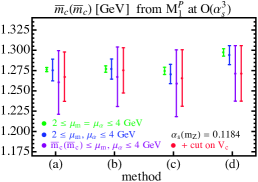
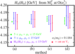
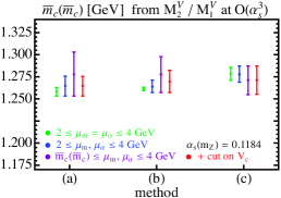
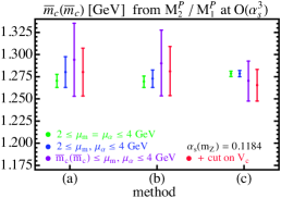
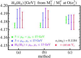
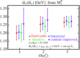
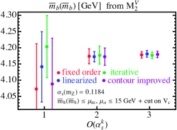
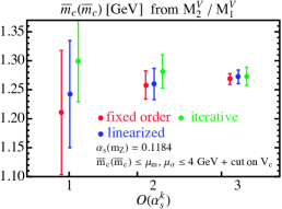
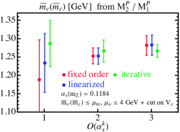
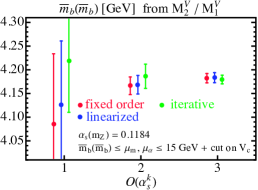
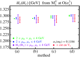
Figure 4: Charm and bottom mass values from the first [second] moment of the vector (a) for charm [(c) for bottom] and pseudoscalar [(b), charm] currents at 𝒪(αs3)𝒪superscriptsubscript𝛼𝑠3\mathcal{O}(\alpha_{s}^{3}); and for the ratio of the second over the first moment for the vector [(d) for charm, (g) for bottom] and pseudoscalar [(e), charm] correlators. We show the outcome of various scale variations for the perturbative expansions (a) – (d) [(a) – (c) for ratios], where green (rightmost) corresponds to 2GeVμm=μα4GeV2GeVsubscript𝜇𝑚subscript𝜇𝛼4GeV2\,{\rm GeV}\leq\mu_{m}=\mu_{\alpha}\leq 4\,{\rm GeV} [5GeVμm=μα15GeV5GeVsubscript𝜇𝑚subscript𝜇𝛼15GeV5\,{\rm GeV}\leq\mu_{m}=\mu_{\alpha}\leq 15\,{\rm GeV} for bottom], blue (second from the left) 2GeVμm,μα4GeVformulae-sequence2GeVsubscript𝜇𝑚subscript𝜇𝛼4GeV2\,{\rm GeV}\leq\mu_{m},\mu_{\alpha}\leq 4\,{\rm GeV} [5GeVμm,μα15GeVformulae-sequence5GeVsubscript𝜇𝑚subscript𝜇𝛼15GeV5\,{\rm GeV}\leq\mu_{m},\mu_{\alpha}\leq 15\,{\rm GeV} for bottom], purple (second from the right) m¯c(m¯c)μm,μα 4GeVformulae-sequencesubscript¯𝑚𝑐subscript¯𝑚𝑐subscript𝜇𝑚subscript𝜇𝛼4GeV\overline{m}_{c}(\overline{m}_{c})\leq\mu_{m},\mu_{\alpha}\leq\,4{\rm GeV} [m¯b(m¯b)μm,μα15GeVformulae-sequencesubscript¯𝑚𝑏subscript¯𝑚𝑏subscript𝜇𝑚subscript𝜇𝛼15GeV\overline{m}_{b}(\overline{m}_{b})\leq\mu_{m},\mu_{\alpha}\leq 15\,{\rm GeV} for bottom] and in red (rightmost) we supplement the latter variation with a cut on the series with larger values of Vcsubscript𝑉𝑐V_{c}.

For example,333The size of the scale variations quoted in this paragraph applies to m¯c(m¯c)subscript¯𝑚𝑐subscript¯𝑚𝑐\overline{m}_{c}(\overline{m}_{c}) as well as to m¯c(3GeV)subscript¯𝑚𝑐3GeV\overline{m}_{c}(3\,{\rm GeV}), and all numerical results are obtained at 𝒪(αs3)𝒪superscriptsubscript𝛼𝑠3{\cal O}(\alpha_{s}^{3}). We also stress that there are no perturbative instabilities concerning the use of the RGE down to the scale m¯c(m¯c)subscript¯𝑚𝑐subscript¯𝑚𝑐\overline{m}_{c}(\overline{m}_{c}). in Ref. Chetyrkin:2009fv method (a) has been used for M1Vsuperscriptsubscript𝑀1𝑉M_{1}^{V} with μm=μαsubscript𝜇𝑚subscript𝜇𝛼\mu_{m}=\mu_{\alpha} varied between 222 and 444 GeV, quoting a perturbative error estimate of 222 MeV. For the expansion methods444To compute the charm and bottom masses in this section we use M1V,exp=0.2121GeV2superscriptsubscript𝑀1𝑉exp0.2121superscriptGeV2M_{1}^{V,\,\rm exp}=0.2121\,{\rm GeV}^{-2} for the charm vector correlator, result obtained in Ref. Dehnadi:2011gc , M1P,latt=0.1402GeV2superscriptsubscript𝑀1𝑃latt0.1402superscriptGeV2M_{1}^{P,\,\rm latt}=0.1402\,{\rm GeV}^{-2} for the charm pseudoscalar correlator, from Ref. Allison:2008xk , and our own computation M2V,exp=2.834×10⁵GeV4superscriptsubscript𝑀2𝑉exp2.834superscript105superscriptGeV4M_{2}^{V,\,{\rm exp}}=2.834\times 10^{-5}\,{\rm GeV}^{-4} for the bottom vector correlator, see Sec. 6. We also use αs(mZ)=0.1184.subscript𝛼𝑠subscript𝑚𝑍0.1184\alpha_{s}(m_{Z})=0.1184. (a) – (d) we obtain for the same scale variation 1.2893±0.0007plus-or-minus1.28930.00071.2893\pm 0.0007, 1.2904±0.0004plus-or-minus1.29040.00041.2904\pm 0.0004, 1.2963±0.0045plus-or-minus1.29630.00451.2963\pm 0.0045 and 1.3009±0.0020plus-or-minus1.30090.00201.3009\pm 0.0020 GeV, respectively, for m¯c(m¯c)subscript¯𝑚𝑐subscript¯𝑚𝑐\overline{m}_{c}(\overline{m}_{c}), which are inconsistent. This can be compared to the corresponding results using independent variations as suggested in Ref. Dehnadi:2011gc . Using 2GeVμα,μm4GeVformulae-sequence2GeVsubscript𝜇𝛼subscript𝜇𝑚4GeV2\,{\rm GeV}\leq\mu_{\alpha},\mu_{m}\leq 4\,{\rm GeV} we obtain 1.291±0.003plus-or-minus1.2910.0031.291\pm 0.003, 1.291±0.003plus-or-minus1.2910.0031.291\pm 0.003, 1.296±0.005plus-or-minus1.2960.0051.296\pm 0.005 and 1.302±0.003plus-or-minus1.3020.0031.302\pm 0.003 GeV, respectively, for expansions (a) – (d). These results are not consistent either. It was furthermore argued in Ref. Dehnadi:2011gc that an adequate variation range should include the charm mass itself (after all, that is the scale that governs the series), motivated by the range 2mc±mcplus-or-minus2subscript𝑚𝑐subscript𝑚𝑐2\,m_{c}\,\pm\,m_{c} around the pair production threshold. Thus, adopting independent scale variation in the range m¯c(m¯c)μm,μα4formulae-sequencesubscript¯𝑚𝑐subscript¯𝑚𝑐subscript𝜇𝑚subscript𝜇𝛼4\overline{m}_{c}(\overline{m}_{c})\leq\mu_{m},\mu_{\alpha}\leq 4 GeV one obtains 1.287±0.018plus-or-minus1.2870.0181.287\pm 0.018, 1.287±0.015plus-or-minus1.2870.0151.287\pm 0.015, 1.282±0.019plus-or-minus1.2820.0191.282\pm 0.019 and 1.291±0.014plus-or-minus1.2910.0141.291\pm 0.014 GeV respectively. The results show consistency and demonstrate the strong dependence on the lower bound of the renormalization scale variation. The outcome is illustrated graphically in Fig. 4, and the order-by-order dependence in Fig. 1 of Ref. Dehnadi:2014kya . In Ref. Dehnadi:2011gc we also explored scale setting in which μmsubscript𝜇𝑚\mu_{m} was fixed to m¯c(m¯c)subscript¯𝑚𝑐subscript¯𝑚𝑐\overline{m}_{c}(\overline{m}_{c}) and only μαsubscript𝜇𝛼\mu_{\alpha} was varied. The outcome is shown in Figs. 4 and 5 of that reference. The contour lines in the μmsubscript𝜇𝑚\mu_{m} – μαsubscript𝜇𝛼\mu_{\alpha} plane for the mass extraction from the first moment of the vector correlator for all methods are shown in Fig. 6 of Ref. Dehnadi:2011gc . The final result quoted in Ref. Dehnadi:2011gc , using αs(mZ)=0.1184± 0.0021subscript𝛼𝑠subscript𝑚𝑍plus-or-minus0.11840.0021\alpha_{s}(m_{Z})=0.1184\,\pm\,0.0021, was m¯c(m¯c)=1.282±(0.006)stat±(0.009)syst±(0.019)pert±(0.010)αs±(0.002)GGsubscript¯𝑚𝑐subscript¯𝑚𝑐plus-or-minus1.282subscript0.006statsubscript0.009systsubscript0.019pertsubscript0.010subscript𝛼𝑠subscript0.002delimited-⟨⟩𝐺𝐺\overline{m}_{c}(\overline{m}_{c})=1.282\,\pm\,(0.006)_{\rm stat}\,\pm\,(0.009)_{\rm syst}\,\pm\,(0.019)_{\rm pert}\,\pm\,(0.010)_{\alpha_{s}}\,\pm\,(0.002)_{\langle GG\rangle}\,GeV based on the iterative expansion method (c).

We have repeated this analysis for the first moment of the pseudoscalar correlator M1Psuperscriptsubscript𝑀1𝑃M_{1}^{P}. Ref. Allison:2008xk uses method (b) with the same scale variation as Ref. Chetyrkin:2009fv , quoting 444 MeV for the truncation error. For methods (a) – (d) and using 2GeVμm=μα4GeV2GeVsubscript𝜇𝑚subscript𝜇𝛼4GeV2\,{\rm GeV}\leq\mu_{m}=\mu_{\alpha}\leq 4\,{\rm GeV} we obtain 1.276±0.003plus-or-minus1.2760.0031.276\pm 0.003, 1.277±0.004plus-or-minus1.2770.0041.277\pm 0.004, 1.275±0.005plus-or-minus1.2750.0051.275\pm 0.005 and 1.297±0.004plus-or-minus1.2970.0041.297\pm 0.004 GeV, respectively. For independent double scale variation between 222 and 444 GeV we obtain, 1.276±0.013plus-or-minus1.2760.0131.276\pm 0.013, 1.277±0.012plus-or-minus1.2770.0121.277\pm 0.012, 1.271±0.012plus-or-minus1.2710.0121.271\pm 0.012 and 1.294±0.012plus-or-minus1.2940.0121.294\pm 0.012 GeV, and if we use m¯c(m¯c)subscript¯𝑚𝑐subscript¯𝑚𝑐\overline{m}_{c}(\overline{m}_{c}) as the lower bound to we obtain 1.260±0.039plus-or-minus1.2600.0391.260\pm 0.039, 1.267±0.037plus-or-minus1.2670.0371.267\pm 0.037 GeV, 1.259±0.041plus-or-minus1.2590.0411.259\pm 0.041 and 1.272±0.034plus-or-minus1.2720.0341.272\pm 0.034. These results are displayed graphically in Fig. 4. The contour lines for the mass extraction from the first moment of the pseudoscalar correlator for all methods are shown in Fig. 2. We see that the results show a qualitative agreement with the situation for the vector current, but at a level of perturbative scale variations that are in general roughly larger by a factor of two.

A similar study can be performed for the extraction of the bottom mass m¯b(m¯b)subscript¯𝑚𝑏subscript¯𝑚𝑏\overline{m}_{b}(\overline{m}_{b}) from the second moment of the vector correlator M2Vsuperscriptsubscript𝑀2𝑉M_{2}^{V}. Ref. Chetyrkin:2009fv uses the fixed-order expansion [method (a)] and correlated scale variation between 5GeVμm=μα15GeV5GeVsubscript𝜇𝑚subscript𝜇𝛼15GeV5\,{\rm GeV}\leq\mu_{m}=\mu_{\alpha}\leq 15\,{\rm GeV}, quoting a perturbative error of 333 MeV. For the same variation we obtain 4.1781±0.0005plus-or-minus4.17810.00054.1781\pm 0.0005, 4.1771±0.0015plus-or-minus4.17710.00154.1771\pm 0.0015, 4.1818±0.0034plus-or-minus4.18180.00344.1818\pm 0.0034 and 4.1792±0.0044plus-or-minus4.17920.00444.1792\pm 0.0044 GeV for methods (a) and (d), respectively. As in the charm case the results are not consistent, but the variations of the results have a much smaller size, as is expected from the fact that for the bottom the renormalization scales are much larger. For independent variation between the same values we get 4.183±0.008plus-or-minus4.1830.0084.183\pm 0.008, 4.181±0.006plus-or-minus4.1810.0064.181\pm 0.006, 4.180±0.006plus-or-minus4.1800.0064.180\pm 0.006 and 4.186±0.013plus-or-minus4.1860.0134.186\pm 0.013 GeV. Finally, if the lower limit of the double variation starts at m¯b(m¯b)subscript¯𝑚𝑏subscript¯𝑚𝑏\overline{m}_{b}(\overline{m}_{b}) we find 4.179±0.011plus-or-minus4.1790.0114.179\pm 0.011, 4.181±0.011plus-or-minus4.1810.0114.181\pm 0.011, 4.175±0.011plus-or-minus4.1750.0114.175\pm 0.011 and 4.184±0.0015plus-or-minus4.1840.00154.184\pm 0.0015 GeV. These results are collected in Fig. 4. The corresponding m¯b(m¯b)subscript¯𝑚𝑏subscript¯𝑚𝑏\overline{m}_{b}(\overline{m}_{b}) contours in the μmsubscript𝜇𝑚\mu_{m} – μαsubscript𝜇𝛼\mu_{\alpha} plane are shown in Fig. 3. As for the charm case, we find fully consistent results for the independent scale variation and using m¯b(m¯b)subscript¯𝑚𝑏subscript¯𝑚𝑏\overline{m}_{b}(\overline{m}_{b}) as the lower bound.

We have also studied the ratio of the first over the second moments for the three cases, and observe a very similar pattern. We do not provide a detailed discussion in the text, but display the outcome graphically in Figs. 4 to 4.

4 Convergence Test

At this point it is useful to consider the perturbative series for all choices of μαsubscript𝜇𝛼\mu_{\alpha} and μmsubscript𝜇𝑚\mu_{m} as different perturbative expansions, which can have different convergence properties. To estimate the perturbative uncertainties one analyzes the outcome of this set of (truncated) series. While the uncorrelated scale variation certainly is a conservative method, one possible concern is that it might lead to an overestimate of the size of the perturbative error. For instance, this might arise for a non-vanishing value of ln(μm/μα)subscript𝜇𝑚subscript𝜇𝛼\ln(\mu_{m}/\mu_{\alpha}) in connection with sizeable values of αs(μα)subscript𝛼𝑠subscript𝜇𝛼\alpha_{s}(\mu_{\alpha}) for μαsubscript𝜇𝛼\mu_{\alpha} close to the charm mass scale, which might artificially spoil the convergence of the expansion. One possible resolution might be to simply reduce the range of scale variation (such as increasing the lower bound). However, this does not resolve the issue, since the resulting smaller variation merely represents a matter of choice. Furthermore, there is in general no guarantee that the series which are left have a better convergence despite the fact that the overall scale variation might become reduced. Preferably, the issue should be fixed from inherent properties of the perturbative series themselves. It is possible to address this issue by supplementing the uncorrelated scale variation method with a convergence test constraint, which we explain in the following.

We implement a finite-order version of the root convergence test. Let us recall that in mathematics, the root test (also known as Cauchy’s radical test) states that for a series of terms ansubscript𝑎𝑛a_{n}, S[a]=nan𝑆delimited-[]𝑎subscript𝑛subscript𝑎𝑛S[a]=\sum_{n}a_{n}, if the quantity Vsubscript𝑉V_{\infty} defined as

Vlim supn(an)1/n,subscript𝑉subscriptlimit-supremum𝑛superscriptsubscript𝑎𝑛1𝑛V_{\infty}\equiv\limsup_{n\to\infty}(a_{n})^{1/n}\,, (15)

is smaller (bigger) than 111, the sum is absolutely convergent (divergent). If Vsubscript𝑉V_{\infty} approaches 111 from above then the series is still divergent, otherwise the test is not conclusive. In Eq. (15) lim suplimit-supremum\limsup stands for the superior limit, which essentially means that in case of oscillating series, one takes the maximum value of the oscillation. In the context of our analysis with truncated series the relevant property is that a smaller Vsubscript𝑉V_{\infty} implies a better convergent series. For the different expansion methods we use, it is simplest to apply the method directly to the sequence of quark masses that are extracted order by order, rewriting the results as a series expansion. Since we only know a finite number of coefficients of the perturbative series, we need to adapt the test. We now introduce Vcsubscript𝑉𝑐V_{c} and proceed as follows: 555One could think of implementing the ratio test as well. However, since we only known a small number of terms, it is likely that one of them becomes close to zero, making one of the ratios blow up. This makes this test very unstable.

  • (a)

    For each pair of renormalization scales (μm,μα)subscript𝜇𝑚subscript𝜇𝛼(\mu_{m},\mu_{\alpha}) we define the convergence parameter Vcsubscript𝑉𝑐V_{c} from the charm mass series m¯c(m¯c)=m(0)+δm(1)+δm(2)+δm(3)subscript¯𝑚𝑐subscript¯𝑚𝑐superscript𝑚0𝛿superscript𝑚1𝛿superscript𝑚2𝛿superscript𝑚3\overline{m}_{c}(\overline{m}_{c})=m^{(0)}+\delta m^{(1)}+\delta m^{(2)}+\delta m^{(3)} resulting from the extractions at 𝒪(αs0,1,2,3)𝒪superscriptsubscript𝛼𝑠0123{\cal O}(\alpha_{s}^{0,1,2,3}):

    Vc=max[δm(1)m(0),(δm(2)m(0))1/2,(δm(3)m(0))1/3].subscript𝑉𝑐𝛿superscript𝑚1superscript𝑚0superscript𝛿superscript𝑚2superscript𝑚012superscript𝛿superscript𝑚3superscript𝑚013V_{c}=\max\!\bigg{[}\frac{\delta m^{(1)}}{m^{(0)}}\,,\Big{(}\frac{\delta m^{(2)}}{m^{(0)}}\Big{)}^{\!\!1/2},\Big{(}\frac{\delta m^{(3)}}{m^{(0)}}\Big{)}^{\!\!1/3}\,\bigg{]}. (16)
  • (b)

    The resulting distribution for Vcsubscript𝑉𝑐V_{c} values can be conveniently cast as a histogram, and the resulting distribution is a measure for the overall convergence of the perturbative expansion being employed. We apply the convergence analysis to the region m¯c(m¯c)μα,μm4formulae-sequencesubscript¯𝑚𝑐subscript¯𝑚𝑐subscript𝜇𝛼subscript𝜇𝑚4\overline{m}_{c}(\overline{m}_{c})\leq\mu_{\alpha},\mu_{m}\leq 4 GeV for charm, and m¯b(m¯b)μα,μm15formulae-sequencesubscript¯𝑚𝑏subscript¯𝑚𝑏subscript𝜇𝛼subscript𝜇𝑚15\overline{m}_{b}(\overline{m}_{b})\leq\mu_{\alpha},\mu_{m}\leq 15 GeV for bottom. If the distribution is peaked around the average Vcdelimited-⟨⟩subscript𝑉𝑐\langle V_{c}\rangle it has a well-defined convergence. Hence discarding series with VcVcmuch-greater-thansubscript𝑉𝑐delimited-⟨⟩subscript𝑉𝑐V_{c}\gg\langle V_{c}\rangle (particularly if they significantly enlarge the estimate of the perturbative error) is justified.
Refer to caption
Refer to caption
Refer to caption
Refer to caption
Refer to caption
Refer to caption
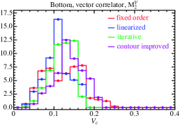
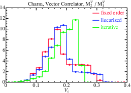
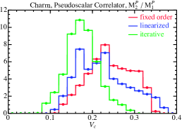
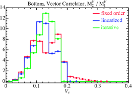
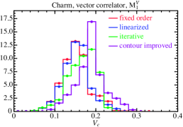
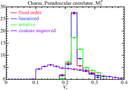
Figure 5: Vcsubscript𝑉𝑐V_{c} distribution for m¯c(m¯c)subscript¯𝑚𝑐subscript¯𝑚𝑐\overline{m}_{c}(\overline{m}_{c}) from the first moment of the vector (a) and pseudoscalar (b) correlator, and for m¯b(m¯b)subscript¯𝑚𝑏subscript¯𝑚𝑏\overline{m}_{b}(\overline{m}_{b}) for the second moment of the vector correlator (c), for expansions (a) – (d). The three lower panels show the same for the ratio of the second over the first moment for expansions (a) – (c).
Refer to caption
Refer to caption
Refer to caption
Refer to caption
Refer to caption
Refer to caption
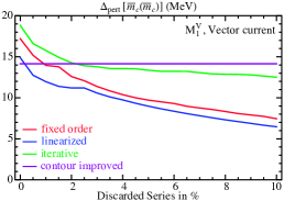
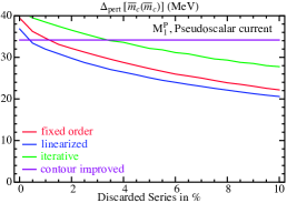
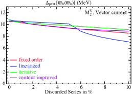
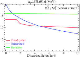
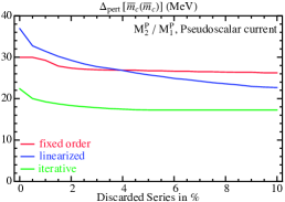
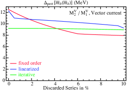
Figure 6: Half of the scale variation of m¯q(m¯q)subscript¯𝑚𝑞subscript¯𝑚𝑞\overline{m}_{q}(\overline{m}_{q}) at 𝒪(αs3)𝒪superscriptsubscript𝛼𝑠3{\mathcal{O}(\alpha_{s}^{3})} as a function of the fraction of the discarded series with highest Vcsubscript𝑉𝑐V_{c} values for the first moment of the vector (a) and pseudoscalar (b) correlators for charm, the second moment of the vector correlator for bottom (c); the ratio of the second over the first moment for the vector [charm (d) and bottom (f)] and pseudoscalar [charm (e)] correlators.

Fig. 5 shows the Vcsubscript𝑉𝑐V_{c} distributions for expansions (a) – (d) for the extraction of the charm mass from the vector moment M1Vsuperscriptsubscript𝑀1𝑉M_{1}^{V}. We find Vcdouble=(0.15, 0.15, 0.17, 0.19)subscriptdelimited-⟨⟩subscript𝑉𝑐double0.150.150.170.19\langle V_{c}\rangle_{\rm double}=(0.15,\,0.15,\,0.17,\,0.19)666Interestingly, the same analysis for the correlated variation with 2GeVμα=μm42GeVsubscript𝜇𝛼subscript𝜇𝑚42\,{\rm GeV}\leq\mu_{\alpha}=\mu_{m}\leq 4 GeV yields Vccorr=(0.14, 0.16, 0.19, 0.19)subscriptdelimited-⟨⟩subscript𝑉𝑐corr0.140.160.190.19\langle V_{c}\rangle_{\rm corr}=(0.14,\,0.16,\,0.19,\,0.19), which is similar to the outcome for the double variation. This same observation can be made for the rest of the correlators. and that the distributions are peaked around Vcdelimited-⟨⟩subscript𝑉𝑐\langle V_{c}\rangle, indicating a very good overall convergence. The scale variation error (defined as half the overall variation) as a function of the fraction of the series (with the largest Vcsubscript𝑉𝑐V_{c} values) that are being discarded is shown in Fig. 6. We see that only around 2% of the series with the highest Vcsubscript𝑉𝑐V_{c} values by themselves cause the increase of the scale variation from well below 151515 MeV to up to 202020 MeV. These series are located at the upper-left and lower-right corners of Figs. 2 and 3, and Fig. 6 of Ref. Dehnadi:2011gc , corresponding to values of μmsubscript𝜇𝑚\mu_{m} and μαsubscript𝜇𝛼\mu_{\alpha} far from each other. Given that these series have very large Vcsubscript𝑉𝑐V_{c} values and do not reflect the overall good convergence behavior of the bulk of the series, it is justified to remove them from the analysis.

The Vcsubscript𝑉𝑐V_{c} distributions for the pseudoscalar first moment M1Psuperscriptsubscript𝑀1𝑃M_{1}^{P} are shown in Fig. 5, again showing a clear peak. However, with Vcdouble=(0.24, 0.24, 0.25, 0.21)subscriptdelimited-⟨⟩subscript𝑉𝑐double0.240.240.250.21\langle V_{c}\rangle_{\rm double}=(0.24,\,0.24,\,0.25,\,0.21) [for correlated variation Vccorr=(0.22, 0.23, 0.22, 0.15)subscriptdelimited-⟨⟩subscript𝑉𝑐corr0.220.230.220.15\langle V_{c}\rangle_{\rm corr}=(0.22,\,0.23,\,0.22,\,0.15) with 222 GeV as the lower bound], the average Vcsubscript𝑉𝑐V_{c} values are significantly larger than for the vector correlator, indicating that the overall perturbative convergence for the pseudoscalar moment is still excellent but worse than for the vector moment. This means that the vector correlator method is superior, and we expect that the perturbative uncertainty in the charm mass from the pseudoscalar is larger. This expectation is indeed confirmed as we discussed in Sec. 3, see also Sec. 9. Fig. 6 shows that the effect of discarding the series with the worst convergence is very similar to that of the vector correlator.

For our determination of the bottom mass we use the second moment M2Vsuperscriptsubscript𝑀2𝑉M_{2}^{V} (see Sec. 6 for a discussion on why we discard the first moment), and employ uncorrelated scale variations in the range m¯b(m¯b)μm,μα15formulae-sequencesubscript¯𝑚𝑏subscript¯𝑚𝑏subscript𝜇𝑚subscript𝜇𝛼15\overline{m}_{b}(\overline{m}_{b})\leq\mu_{m},\mu_{\alpha}\leq 15 GeV. Fig. 5 shows the corresponding histograms, and we find that the convergence test yields Vcdouble=(0.13, 0.11, 0.12, 0.15)subscriptdelimited-⟨⟩subscript𝑉𝑐double0.130.110.120.15\langle V_{c}\rangle_{\rm double}=(0.13,\,0.11,\,0.12,\,0.15) for expansions (a) – (d) [for the correlated variation with scales set equal and 5GeVμα=μm155GeVsubscript𝜇𝛼subscript𝜇𝑚155\,{\rm GeV}\leq\mu_{\alpha}=\mu_{m}\leq 15 GeV we find Vccorr=(0.13, 0.09, 0.13, 0.15)subscriptdelimited-⟨⟩subscript𝑉𝑐corr0.130.090.130.15\langle V_{c}\rangle_{\rm corr}=(0.13,\,0.09,\,0.13,\,0.15)]. As expected, the averages for the bottom are much smaller than for the charm. We further find that discarding series with the highest Vcsubscript𝑉𝑐V_{c} values only has minor effects on the perturbative error estimate for fractions up to 5%percent55\%, see Fig 6. This is a confirmation that the series for bottom moments overall are more stable, which is again expected from the fact that perturbation theory should work better for the bottom than for the lighter charm.

The behavior of the ratios of moments is very similar as that for regular moments, as can be seen in Figs. 6 and 5, panels (d) – (f). We find the following average values for Vcsubscript𝑉𝑐V_{c} for methods (a) – (d): ratios of charm vector moments Vcdouble=(0.19, 0.18, 0.19)subscriptdelimited-⟨⟩subscript𝑉𝑐double0.190.180.19\langle V_{c}\rangle_{\rm double}=(0.19,\,0.18,\,0.19) [Vccorr=(0.16, 0.16, 0.23)subscriptdelimited-⟨⟩subscript𝑉𝑐corr0.160.160.23\langle V_{c}\rangle_{\rm corr}=(0.16,\,0.16,\,0.23)]; ratios of charm pseudoscalar moments Vcdouble=(0.25, 0.23, 0.18)subscriptdelimited-⟨⟩subscript𝑉𝑐double0.250.230.18\langle V_{c}\rangle_{\rm double}=(0.25,\,0.23,\,0.18) [Vccorr=(0.25, 0.20, 0.16)subscriptdelimited-⟨⟩subscript𝑉𝑐corr0.250.200.16\langle V_{c}\rangle_{\rm corr}=(0.25,\,0.20,\,0.16)]; ratios of bottom vector moments Vcdouble=(0.13, 0.12, 0.13)subscriptdelimited-⟨⟩subscript𝑉𝑐double0.130.120.13\langle V_{c}\rangle_{\rm double}=(0.13,\,0.12,\,0.13) [Vccorr=(0.13, 0.11, 0.14)subscriptdelimited-⟨⟩subscript𝑉𝑐corr0.130.110.14\langle V_{c}\rangle_{\rm corr}=(0.13,\,0.11,\,0.14)]. Therefore we conclude that the perturbative convergence of the ratios of moments is in general terms a bit worse than that of regular moments, except for the linearized iterative method of the pseudoscalar ratios.

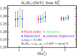
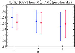
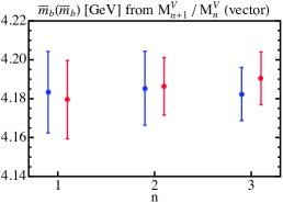
In our final numerical analyses we discard 333% of the series with the worst Vcsubscript𝑉𝑐V_{c} values. As can be seen from Fig. 5, this only affects series with Vcsubscript𝑉𝑐V_{c} values much larger than the average values for the whole set of series. It is our intention to keep the fraction of discarded series as small as possible, since it is our aim to remove only series with convergence properties that are obviously much worse than those of the bulk of the series. We call this procedure trimming in the following. As we see in Figs. 7, the results including the trimming show a very good order-by-order convergence for the heavy quark mass determinations, and at each order every expansion method gives consistent results for the central values as well as for the estimate of the perturbative uncertainties. Figs. 7 and 7 show the results for m¯c(m¯c)subscript¯𝑚𝑐subscript¯𝑚𝑐\overline{m}_{c}(\overline{m}_{c}) from the vector and pseudoscalar correlators, respectively, for expansions (a) – (d) at 𝒪(αs1,2,3)𝒪superscriptsubscript𝛼𝑠123{\cal O}(\alpha_{s}^{1,2,3}) and with m¯c(m¯c)μm,μα4formulae-sequencesubscript¯𝑚𝑐subscript¯𝑚𝑐subscript𝜇𝑚subscript𝜇𝛼4\overline{m}_{c}(\overline{m}_{c})\leq\mu_{m},\mu_{\alpha}\leq 4 GeV, using the first moment. Figs. 7 and 7 show results for methods (a) – (c), using the ratio of the second over the first moment. Analogously, Figs. 7 and 7 show the results for m¯b(m¯b)subscript¯𝑚𝑏subscript¯𝑚𝑏\overline{m}_{b}(\overline{m}_{b}) for the second moment, and the ratio of the second over the first moment, respectively, with the uncorrelated variation m¯b(m¯b)μm,μα15formulae-sequencesubscript¯𝑚𝑏subscript¯𝑚𝑏subscript𝜇𝑚subscript𝜇𝛼15\overline{m}_{b}(\overline{m}_{b})\leq\mu_{m},\mu_{\alpha}\leq 15 GeV.

Refer to caption
Refer to caption
Refer to caption
Refer to caption
Refer to caption
Refer to caption
Figure 7: Charm and bottom mass values from the first [second] moment of the vector (a) for charm [(c) for bottom] and pseudoscalar [(b), charm] currents at 𝒪(αs1,2,3)𝒪superscriptsubscript𝛼𝑠123\mathcal{O}(\alpha_{s}^{1,2,3}); and for the ratio of the second over the first moment for the vector [(d) for charm, (g) for bottom] and pseudoscalar [(e), charm] correlators for expansions (a) – (d) [(a) – (c) for ratios], in red, blue, green and purple, respectively.

5 Lattice Simulation Data

The pseudoscalar current is not realized in nature in a way which is useful to compute the moments of the corresponding correlator from experimental data. Results for the moments of the pseudoscalar current correlator can, however, be obtained from simulations on the lattice. The strategy of these numerical simulations is to tune the lattice parameters (such as bare coupling constant and masses) to a selected number of observables (e.g. the energy splitting of ΥΥ\Upsilon resonances). Once this tuning is performed, the lattice action is fully specified and no further changes are implemented. The tuned lattice action can then be used to perform all sorts of predictions, moments of correlators among them. Lattice simulations have to face a number of challenges, which usually translate into sizeable uncertainties. Among those are the extrapolations to the infinite volume and the zero lattice spacing (the latter being much harder), as well as the extrapolation to physical quark masses. On top of these systematic uncertainties, there are also statistical ones, which are related to the finite sampling used to perform the path integrations. On the other hand there are also concerns on the type of lattice action which is being used for the fermions. According to Ref. Allison:2008xk , the moments of the pseudoscalar correlator are least affected by systematic uncertainties, and so HPQCD has focused on those for their subsequent high-precision analyses.

To the best of our knowledge, HPQCD is the only lattice collaboration which has published results on QCD correlators. They have used the staggered-quarks lattice action, and MILC configurations for gluons. These results have been used to determine the charm mass and the strong coupling constant Allison:2008xk ; McNeile:2010ji ; Chakraborty:2014aca with high accuracy, as well as the bottom mass McNeile:2010ji ; Colquhoun:2014ica , with smaller precision. We will use the simulation results as given in Ref. Allison:2008xk , even if the results quoted in of McNeile:2010ji ; Chakraborty:2014aca are a bit more precise. The reason for this choice is that while Allison:2008xk makes a straightforward extrapolation to the continuum, which is independent of the charm mass and αssubscript𝛼𝑠\alpha_{s} extractions, in McNeile:2010ji ; Chakraborty:2014aca the fit for the quark masses, the strong coupling constant and the extrapolation to the continuum is performed all at once, in a single fit. Furthermore that fits contains a lot of priors for the parameters one is interested in fitting. In any case, as we have seen, the charm mass extraction from the pseudoscalar correlator is dominated by perturbative uncertainties, as a result of the bad convergence of the series expansion for its moments.

Ref. Allison:2008xk provides simulation results for the so-called reduced moments Rksubscript𝑅𝑘R_{k}, which are collected in their Table II. The index k𝑘k takes only even values, and starts with the value k=4𝑘4k=4, which is fairly insensitive to the charm mass. Hence the lowest moment we consider is R6subscript𝑅6R_{6}. Reduced moments are defined as (up to a global power) the full moment divided by the tree-level result. By taking this ratio, the authors of Ref. Allison:2008xk claim that large cancellations between systematic errors take place. The reduced moments are scaleless, and the mass-dimension that one obviously needs to determinate the charm quark mass is regained by dividing with the mass of the ηcsubscript𝜂𝑐\eta_{c} pseudoscalar particle. Thus one can easily translate the reduced moments into the more familiar correlator moments MnPsuperscriptsubscript𝑀𝑛𝑃M_{n}^{P} with the following relation:

MnP=[CP(nf=4)]n,00,0(R2n+4mηc)2n,superscriptsubscript𝑀𝑛𝑃subscriptsuperscriptdelimited-[]subscript𝐶𝑃subscript𝑛𝑓400𝑛0superscriptsubscript𝑅2𝑛4subscript𝑚subscript𝜂𝑐2𝑛M_{n}^{P}=[C_{P}(n_{f}=4)]^{0,0}_{n,0}\bigg{(}\dfrac{R_{2n+4}}{m_{\eta_{c}}}\bigg{)}^{\!2n}\,, (17)

where the CPsubscript𝐶𝑃C_{P} coefficients correspond to the tree-level terms of the standard fixed-order expansion of Eq. (5). Although the experimental value for ηcsubscript𝜂𝑐\eta_{c} is 2.9836(7)2.983672.9836(7)\,GeV, we use the value mηc=2.980subscript𝑚subscript𝜂𝑐2.980m_{\eta_{c}}=2.980\,GeV given in Ref. Allison:2008xk , in order to ease comparison with that analysis. In Ref. Chakraborty:2014aca the value mηc=2.9863(27)subscript𝑚subscript𝜂𝑐2.986327m_{\eta_{c}}=2.9863(27)\,GeV is used. It is claimed that (as for the lattice action) it has no QED effects, and the error accounts for cc¯𝑐¯𝑐c\bar{c} annihilation. Using the quote in Ref. Chakraborty:2014aca changes M1Psuperscriptsubscript𝑀1𝑃M_{1}^{P} by 0.4%percent0.40.4\% and the effect on the charm mass is of the order of 222 MeV. The uncertainty in the ηcsubscript𝜂𝑐\eta_{c} mass has no effect on the MnPsuperscriptsubscript𝑀𝑛𝑃M_{n}^{P} errors. In Table 1 we quote the lattice simulation results written as regular moments MnPsuperscriptsubscript𝑀𝑛𝑃M_{n}^{P}.

M1Psuperscriptsubscript𝑀1𝑃M_{1}^{P} M2Psuperscriptsubscript𝑀2𝑃M_{2}^{P} M3Psuperscriptsubscript𝑀3𝑃M_{3}^{P} M4Psuperscriptsubscript𝑀4𝑃M_{4}^{P}
1.402(20)1.402201.402(20) 1.361(40)1.361401.361(40) 1.426(59)1.426591.426(59) 1.558(89)1.558891.558(89)
Table 1: Lattice simulation results for the moments of the twice-subtracted pseudoscalar correlator P(q2)𝑃superscript𝑞2P(q^{2}) for nf=4subscript𝑛𝑓4n_{f}=4. Moments given in units of 10n×10^{-n}\times GeV-2n.

6 Computation of the Experimental Moments for the Bottom Correlator

In this section we present our computation of the moments for the bottom vector current correlator from experimental data. These are made of three distinct contributions: the narrow resonances below threshold, the region of broader resonances, explored by BABAR :2008hx , and the continuum region, where no data has been taken and some modeling is required. The BABAR data has to be corrected for initial-state radiation and vacuum polarization effects. In the continuum region we use a model which consists of a combination of a linear fit to the BaBar experimental points with energy larger than 11.0511.0511.05\,GeV, and perturbation theory as a model for missing experimental data, which are joined smoothly by a cubic interpolation. We assign a conservative uncertainty guided by the error function of the linear fit to the BABAR data in the region with measurements with the highest energy. Our determination of the experimental bottom moments differs from Ref. Chetyrkin:2009fv in the way we model the uncertainties for the hadronic cross section in the continuum region, plus other minor differences in the contributions from the narrow widths and the threshold region, see discussion in Sec. 7. We also provide the correlation matrix among different moments, which cannot be found in the literature. Therefore, even though there are some similarities with the computations outlined in Chetyrkin:2009fv , we find it justified to discuss our computation of the experimental moments in some detail.

We note that our results for the moments of the bottom vector current correlator have already been used in the analyses of high-n𝑛n moments of Ref. Hoang:2012us , in the context of nonrelativistic large-n𝑛n sum rules.

6.1 Narrow Resonances

The contribution of resonances below the open bottom threshold s=10.62GeV𝑠10.62GeV\sqrt{s}=10.62\,\rm{GeV} includes Υ(1S)Υ1𝑆\Upsilon(1S) up to Υ(4S)Υ4𝑆\Upsilon(4S). We use the narrow width approximation to compute their contribution to the experimental moments, finding

Mnres=9πΓeeα(MΥ)2MΥ2n+1.superscriptsubscript𝑀𝑛res9𝜋subscriptΓ𝑒𝑒𝛼superscriptsubscript𝑀Υ2superscriptsubscript𝑀Υ2𝑛1M_{n}^{\rm res}=\frac{9\pi\Gamma_{ee}}{\alpha(M_{\Upsilon})^{2}M_{\Upsilon}^{2n+1}}\,. (18)

The masses and electronic widths of these four resonances are taken from the PDG Agashe:2014kda , and the values of the effective electromagnetic coupling constant evaluated at the ΥΥ\Upsilon masses are taken from Ref. Kuhn:2007vp . This information is collected in Table 2. We have also checked that if one uses a Breit-Wigner instead of the narrow width approximation the results change by an amount well within the error due to the uncertainty in the electronic width.

In analogy to what we found in our study of the charm moments Dehnadi:2011gc , the effect of the mass uncertainty in the moments is negligible. Therefore one only needs to consider the experimental uncertainty in the electronic widths. There is no information on the correlation between the measurements of these widths. The PDG averages of the electronic partial widths for the first three resonances is dominated by the CLEO measurement Rosner:2005eu .777Refs. Kuhn:2007vp ; Chetyrkin:2009fv assume that the error of the electronic width for the first three narrow resonances is 100%percent100100\% correlated, and uncorrelated to that of the Υ(4S)Υ4𝑆\Upsilon(4S). Therefore we take the approach that half of the width’s uncertainty (in quadrature) is uncorrelated (therefore mainly of statistical origin), whereas the other half is correlated among the various resonances (therefore coming from common systematics in the measurements).

Υ(1S)Υ1𝑆\Upsilon(1S) Υ(2S)Υ2𝑆\Upsilon(2S) Υ(3S)Υ3𝑆\Upsilon(3S) Υ(4S)Υ4𝑆\Upsilon(4S)
MΥ(GeV)subscript𝑀ΥGeVM_{\Upsilon}(\rm{GeV}) 9.46030(26) 10.02326(31) 10.3552(5) 10.5794(12)
Γee(KeV)subscriptΓeeKeV\Gamma_{\rm{ee}}(\rm{KeV}) 1.340(18) 0.612(11) 0.443(8) 0.272(29)
(αQEDα(MΥ))2superscriptsubscript𝛼QED𝛼subscript𝑀Υ2\Big{(}\frac{\alpha_{\rm QED}}{\alpha(M_{\Upsilon})}\Big{)}^{\!2} 0.932069 0.93099 0.930811 0.930093
Table 2: Masses and electronic widths of narrow ΥΥ\Upsilon resonances Agashe:2014kda and effective electromagnetic coupling constant Kuhn:2007vp . αQED=1/137.035999084(51)subscript𝛼QED1137.03599908451\alpha_{\rm QED}=1/137.035999084(51) represents the fine structure constant.

6.2 Threshold Region

The region between the open bottom threshold and the experimental measurement of the Rbsubscript𝑅𝑏R_{b}-ratio at the highest energy, 10.62GeVs11.2062GeV10.62GeVs11.2062GeV10.62\,\rm{GeV}\leq\sqrt{s}\leq 11.2062\,{\rm GeV}, is referred to as the threshold region. The region above the last experimental measurement will be collectively denoted as the continuum region. The first experimental data close to the B meson threshold were taken by the CLEO Ammar:1997sk ; Besson:1984bd ; Huang:2006em and CUSB Lovelock:1985nb collaborations. The measurements at each c.m. energy have a 6%percent66\% systematic uncertainty. More recently the BABAR collaboration :2008hx has measured the Rbsubscript𝑅𝑏R_{b}-ratio in the energy region between 10.54GeV10.54GeV10.54\,\rm{GeV} and 11.20GeV11.20GeV11.20\,\rm{GeV}, with significantly higher statistics and better control of systematic uncertainties (of the order of 3%percent33\%). These measurements are taken in small energy bins, densely populating the threshold region. The BABAR data supersedes the older data of CLEO and CUSB, and it has already been used in Refs. Chetyrkin:2009fv ; Chetyrkin:2010ic ; Bodenstein:2012 , in which the bottom mass was also determined.

This BABAR data for the Rbsubscript𝑅𝑏R_{b}-ratio has not been corrected for initial-state radiation and vacuum polarization effects. Moreover, the effect of the Υ(4S)Υ4𝑆\Upsilon(4S) resonance has not been subtracted,888The radiative tails of the first three resonances are provided by BABAR, so they can be subtracted at the data level, before correcting for vacuum polarization effects. so we have performed the subtraction ourselves, using the Breit-Wigner approximation and using for the total width the PDG value Γ4S=20.5subscriptΓ4𝑆20.5\Gamma_{4S}=20.5 MeV:

RBW(s)=9M4S2Γee4Sα(M4S)2Γ4S(sM4S2)2+Γ4S2M4S2.superscript𝑅BW𝑠9superscriptsubscript𝑀4𝑆2subscriptsuperscriptΓ4𝑆ee𝛼superscriptsubscript𝑀4𝑆2subscriptΓ4𝑆superscript𝑠superscriptsubscript𝑀4𝑆22superscriptsubscriptΓ4𝑆2superscriptsubscript𝑀4𝑆2R^{\rm{BW}}(s)=\frac{9\,M_{4S}^{2}\,\Gamma^{4S}_{\rm{ee}}}{\alpha(M_{4S})^{2}}\frac{\Gamma_{4S}}{(s-M_{4S}^{2})^{2}+\Gamma_{4S}^{2}M_{4S}^{2}}\,. (19)

For the subtraction of the Υ(4S)Υ4𝑆\Upsilon(4S) resonance and the correction for the initial state radiation we take an approach similar to Ref. Chetyrkin:2009fv .

6.2.1 Subtraction of the Υ(4S)Υ4𝑆\Upsilon(4S) Radiative Tail

Before subtracting the radiative tail of the Υ(4S)Υ4𝑆\Upsilon(4S) resonance one has to account for vacuum polarization effects. BaBar experimental data has been normalized to the theoretical Born level dimuon cross section (using the fine structure constant rather than the running effective electromagnetic coupling), instead of normalizing to the number of events with muons in the final state. Therefore one has to multiply the BaBar data with [α(s)/αem]2superscriptdelimited-[]𝛼𝑠subscript𝛼em2[\alpha(s)/\alpha_{\rm em}]^{2}, which we take as constant with value 0.930.930.93.

The contribution to be subtracted from the BABAR data (already corrected for vacuum polarization effects) is the ISR-distorted tail of the Υ(4S)Υ4𝑆\Upsilon(4S), which reaches to energies above its mass. The cross section R𝑅R and the ISR-distorted cross-section R^^𝑅\hat{R} are related by a convolution relation

R^(s)=z01dzzG(z,s)R(sz),^𝑅𝑠superscriptsubscriptsubscript𝑧01d𝑧𝑧𝐺𝑧𝑠𝑅𝑠𝑧\hat{R}(s)=\int_{z_{0}}^{1}\dfrac{{\rm d}z}{z}\,G(z,s)\ R(s\,z)\,, (20)

which can be used to determine the ISR effects on the Υ(4S)Υ4𝑆\Upsilon(4S) resonance given in Eq. (19). Here the lower integration bound is z0=(10GeV)2/ssubscript𝑧0superscript10GeV2sz_{0}=(10\,\rm{GeV})^{2}/s. This value is not fully fixed by theoretical arguments, and it is chosen such that it excludes the narrow resonances, but keeps the major part of the Υ(4S)Υ4𝑆\Upsilon(4S) line shape. The radiator function G𝐺G is given as Jadach:1988gb ; Chetyrkin:1996tz

G(z,s)𝐺𝑧𝑠\displaystyle G(z,s) =(1z)β(s) 1G~(z,s),absentsuperscript1𝑧𝛽𝑠1~𝐺𝑧𝑠\displaystyle=(1-z)^{\beta(s)\,-\,1}\,\tilde{G}(z,s)\,, (21)
G~(z,s)~𝐺𝑧𝑠\displaystyle\widetilde{G}(z,s) =β(s)eδyfs(s)F(s)[δCV+S(s)+δCH(s,z)],absent𝛽𝑠superscript𝑒subscript𝛿yfss𝐹𝑠delimited-[]superscriptsubscript𝛿𝐶𝑉𝑆𝑠superscriptsubscript𝛿𝐶𝐻𝑠𝑧\displaystyle=\beta(s)\,e^{\delta_{\rm{yfs}(s)}}\,F(s)\big{[}\,\delta_{C}^{V+S}(s)+\delta_{C}^{H}(s,z)\,\big{]}\,,

where the specific form of β𝛽\beta, F𝐹F and the two δ𝛿\delta’s can be found in Eq. (7) of Chetyrkin:2009fv . Note that the function G(z,s)𝐺𝑧𝑠G(z,s) is divergent as z1𝑧1z\rightarrow 1, but since 0<β1<10𝛽110<\beta-1<-1, it is integrable. The divergent behavior is absent in G~~𝐺\widetilde{G}, which in the limit z1𝑧1z\rightarrow 1 reduces to

G~(1,s)=β(s)eδyfs(s)F(s)δCV+S(s).~𝐺1𝑠𝛽𝑠superscript𝑒subscript𝛿yfs𝑠𝐹𝑠superscriptsubscript𝛿𝐶𝑉𝑆𝑠\widetilde{G}(1,s)\,=\,\beta(s)\,e^{\delta_{\rm{yfs}}(s)}\,F(s)\,\delta_{C}^{V+S}(s)\,. (22)

After subtracting the radiative tail of the Υ(4S)Υ4𝑆\Upsilon(4S) we find that to a good approximation the cross section vanishes for energies below 10.62GeV10.62GeV10.62\,\rm{GeV}. Therefore we add an additional point to our BABAR dataset: Rb(10.62GeV)=0subscript𝑅𝑏10.62GeV0R_{b}(10.62\,\rm{GeV})=0 and take Rb=0subscript𝑅𝑏0R_{b}=0 for energies below 10.6210.6210.62 GeV. Since the subtracted cross section does not exactly vanish between 10.540810.540810.5408 GeV and 10.6210.6210.62 GeV, we take the (small) contribution of the subtracted cross section in that region to the moments as an additional source of systematic correlated uncertainty.

6.2.2 Deconvolution of Initial-State Radiation

After subtraction of the radiative tails and correcting for vacuum polarization effects, the BABAR threshold data are corrected for ISR. The inversion of the convolution in Eq. (20), can be carried out in an iterative way Chetyrkin:2009fv . Defining δG(z,s)=G(z,s)δ(1z)𝛿𝐺𝑧𝑠𝐺𝑧𝑠𝛿1𝑧\delta G(z,s)\,=\,G(z,s)\,-\,\delta(1-z) one can use a successive series of approximations

Rj(s)=R0(s)z01dzzδG(z,s)Rj1(sz),superscript𝑅𝑗𝑠superscript𝑅0𝑠superscriptsubscriptsubscript𝑧01d𝑧𝑧𝛿𝐺𝑧𝑠superscript𝑅𝑗1𝑠𝑧R^{j}(s)=R^{0}(s)-\int_{z_{0}}^{1}\,\dfrac{{\rm d}z}{z}\,\delta G(z,s)\,R^{j-1}(s\,z), (23)

where we denoted the j𝑗j-th approximation of R(s)𝑅𝑠R(s) as Rj(s)superscript𝑅𝑗𝑠R^{j}(s) and use as starting point R0(s)=R^(s)superscript𝑅0𝑠^𝑅𝑠R^{0}(s)=\hat{R}(s), the BABAR data after correcting for vacuum polarization effects and subtracting the radiative tails. In Eq. (23) we take z0=(10.62GeV)2/ssubscript𝑧0superscript10.62GeV2sz_{0}=(10.62\,\rm{GeV})^{2}/s, using as a starting point the energy value for which the cross section vanishes after the subtraction of the radiative tails. To isolate the singularity at the higher endpoint one can perform a subtraction at z=1𝑧1z=1, resulting in:

Rj(s)superscript𝑅𝑗𝑠\displaystyle R^{j}(s) =\displaystyle= R0(s)+Rj1(s)z01dzz(1z)β(s) 1[G~(z,s)Rj1(sz)zG~(1,s)Rj1(s)]superscript𝑅0𝑠superscript𝑅𝑗1𝑠superscriptsubscriptsubscript𝑧01d𝑧𝑧superscript1𝑧𝛽𝑠1delimited-[]~𝐺𝑧𝑠superscript𝑅𝑗1𝑠𝑧𝑧~𝐺1𝑠superscript𝑅𝑗1𝑠\displaystyle R^{0}(s)+R^{j-1}(s)-\int_{z_{0}}^{1}\dfrac{{\rm d}z}{z}\,\,\big{(}1-z\big{)}^{\beta(s)\,-\,1}\,\Big{[}\widetilde{G}(z,s)\,R^{j-1}(s\,z)-z\,\widetilde{G}(1,s)\,R^{j-1}(s)\Big{]} (24)
\displaystyle- 1β(s)G~(1,s)Rj1(s)(1z0)β(s).1𝛽𝑠~𝐺1𝑠superscript𝑅𝑗1𝑠superscript1subscript𝑧0𝛽𝑠\displaystyle\frac{1}{\beta(s)}\,\widetilde{G}(1,s)\,R^{j-1}(s)\big{(}1-z_{0}\big{)}^{\beta(s)}\,.

We use the trapezoidal rule to evaluate the integration on the discrete set of experimental data measurements labeled by the index i𝑖i. Changing the integration variable from z𝑧z to energy we find

Rij=Ri0+Rij1+G~(1,Ei2)Rij1(1E12Ei2)β(Ei2)(E1(E2E1)Ei2E121β(Ei2))subscriptsuperscript𝑅𝑗𝑖subscriptsuperscript𝑅0𝑖subscriptsuperscript𝑅𝑗1𝑖~𝐺1superscriptsubscript𝐸𝑖2superscriptsubscript𝑅𝑖𝑗1superscript1superscriptsubscript𝐸12superscriptsubscript𝐸𝑖2𝛽superscriptsubscript𝐸𝑖2subscript𝐸1subscript𝐸2subscript𝐸1superscriptsubscript𝐸𝑖2superscriptsubscript𝐸121𝛽superscriptsubscript𝐸𝑖2\displaystyle R^{j}_{i}=R^{0}_{i}+R^{j-1}_{i}+\widetilde{G}(1,E_{i}^{2})R_{i}^{j-1}\Bigg{(}1-\frac{E_{1}^{2}}{E_{i}^{2}}\Bigg{)}^{\!\beta(E_{i}^{2})}\Bigg{(}\frac{E_{1}(E_{2}-E_{1})}{E_{i}^{2}-E_{1}^{2}}-\frac{1}{\beta(E_{i}^{2})}\Bigg{)} (25)
k=2i1(1Ek2Ei2)β(Ei2) 1Ek[G~(Ek2Ei2,Ei2)Rkj1Ek2G~(1,Ei2)Rij1Ei2](Ek+1Ek1),superscriptsubscript𝑘2𝑖1superscript1superscriptsubscript𝐸𝑘2superscriptsubscript𝐸𝑖2𝛽superscriptsubscript𝐸𝑖21subscript𝐸𝑘delimited-[]~𝐺superscriptsubscript𝐸𝑘2superscriptsubscript𝐸𝑖2superscriptsubscript𝐸𝑖2superscriptsubscript𝑅𝑘𝑗1superscriptsubscript𝐸𝑘2~𝐺1superscriptsubscript𝐸𝑖2superscriptsubscript𝑅𝑖𝑗1superscriptsubscript𝐸𝑖2subscript𝐸𝑘1subscript𝐸𝑘1\displaystyle-\sum_{k=2}^{i-1}\Bigg{(}1-\frac{E_{k}^{2}}{E_{i}^{2}}\Bigg{)}^{\!\beta(E_{i}^{2})\,-\,1}\!E_{k}\Bigg{[}\widetilde{G}\Bigg{(}\frac{E_{k}^{2}}{E_{i}^{2}},E_{i}^{2}\Bigg{)}\frac{R_{k}^{j-1}}{E_{k}^{2}}-\widetilde{G}(1,E_{i}^{2})\frac{R_{i}^{j-1}}{E_{i}^{2}}\Bigg{]}(E_{k+1}-E_{k-1})\,,

where we have used R1j=R(10.62GeV)0superscriptsubscript𝑅1𝑗𝑅10.62GeV0R_{1}^{j}=R(10.62\,\rm{GeV})\equiv 0 for all iterations. After applying the procedure as many times as necessary to obtain a stable solution, one obtains the ISR-corrected cross section. Among the experimental measurements one finds two data points taken at very similar values of the energy: 10.8610.8610.86 GeV and 10.860510.860510.8605 GeV. It turns out that the fact that they lie very close makes the iterative procedure unstable. Therefore we drop the latter point from our analysis.

In Fig. 8 we show the BABAR data after the subtraction of all radiative tails, before (red) and after (blue) ISR and vacuum polarization corrections.
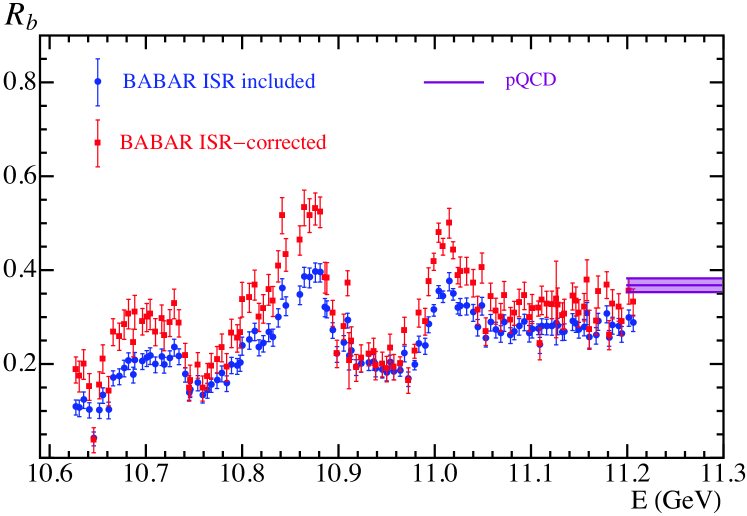
Refer to caption
Figure 8: BABAR experimental data before (blue) and after (red) the ISR correction is applied. The purple bar on the right refers to the pQCD prediction for the continuum region. We have removed one data point at E=10.8605𝐸10.8605E=10.8605 GeV.

6.2.3 Determination of the Unfolding Error Matrix

The BABAR collaboration splits the experimental uncertainties into statistical, systematic uncorrelated, and systematic correlated. We add the two former in quadrature to obtain the total uncorrelated uncertainty ϵuncorsuperscriptitalic-ϵuncor\epsilon^{\rm uncor} and rename the latter as the total correlated uncertainty ϵcorsuperscriptitalic-ϵcor\epsilon^{\rm{cor}}. The removal of the radiative tails of the ΥΥ\Upsilon mesons has no effect on these uncertainties. Therefore, the correlation matrix for the BABAR data after the subtraction of the radiative tails, before it is corrected for ISR effects, can be written as

Mij0 0=(ϵiuncor)2δij+ϵicorϵjcor.subscriptsuperscript𝑀00𝑖𝑗superscriptsuperscriptsubscriptitalic-ϵ𝑖uncor2subscript𝛿𝑖𝑗subscriptsuperscriptitalic-ϵcor𝑖subscriptsuperscriptitalic-ϵcor𝑗M^{0\,0}_{ij}=(\epsilon_{i}^{\rm{uncor}})^{2}\,\delta_{ij}+\epsilon^{\rm{cor}}_{i}\epsilon^{\rm{cor}}_{j}\,. (26)

One needs to compute a new correlation matrix after each iteration. In this way we determine the unfolding error matrix.

The master formula in Eq. (25) can be cast in a matrix form as follows:

Rij=Ri0+k=2iGikRkj1,subscriptsuperscript𝑅𝑗𝑖subscriptsuperscript𝑅0𝑖superscriptsubscript𝑘2𝑖subscript𝐺𝑖𝑘superscriptsubscript𝑅𝑘𝑗1R^{j}_{i}=R^{0}_{i}+\sum_{k=2}^{i}G_{ik}R_{k}^{j-1}\,, (27)

where Rijsubscriptsuperscript𝑅𝑗𝑖R^{j}_{i} is to be thought as the i𝑖i-th component of the column vector Rjsuperscript𝑅𝑗R^{j}, and Giksubscript𝐺𝑖𝑘G_{ik} represents the (i,k)𝑖𝑘(i,k)-component of a matrix G𝐺G. Here Rijsuperscriptsubscript𝑅𝑖𝑗R_{i}^{j} depends only on the initial value Ri0superscriptsubscript𝑅𝑖0R_{i}^{0} and the result of the previous iteration Rij1superscriptsubscript𝑅𝑖𝑗1R_{i}^{j-1}. The Giksubscript𝐺𝑖𝑘G_{ik} do not depend on Rkjsuperscriptsubscript𝑅𝑘𝑗R_{k}^{j} or the iteration step j𝑗j. Therefore, for the error propagation one uses

RijRk0=δik,RijRkj1=Gik,formulae-sequencesubscriptsuperscript𝑅𝑗𝑖subscriptsuperscript𝑅0𝑘subscript𝛿𝑖𝑘subscriptsuperscript𝑅𝑗𝑖subscriptsuperscript𝑅𝑗1𝑘subscript𝐺𝑖𝑘\frac{\partial R^{j}_{i}}{\partial R^{0}_{k}}=\delta_{ik}\,,\qquad\frac{\partial R^{j}_{i}}{\partial R^{j-1}_{k}}=G_{ik}\,, (28)

both of them j𝑗j-independent. We will denote with Mjjsuperscript𝑀𝑗𝑗M^{j\,j} the correlation matrix among the entries of the vector Rjsuperscript𝑅𝑗R^{j} for a given iteration j𝑗j. We also find it convenient to introduce the correlation matrix among Rjsuperscript𝑅𝑗R^{j} and R0superscript𝑅0R^{0}, referred to as Mj 0superscript𝑀𝑗 0M^{j\,0}. Finally we use the notation M0j(Mj 0)Tsuperscript𝑀0𝑗superscriptsuperscript𝑀𝑗 0𝑇M^{0\,j}\equiv(M^{j\,0})^{T}. We find for the correlation matrix after j𝑗j iterations:

Mjjsuperscript𝑀𝑗𝑗\displaystyle M^{j\,j} =M0 0+M0j1GT+GM(j1) 0+GM(j1)(j1)GT,absentsuperscript𝑀00superscript𝑀0𝑗1superscript𝐺𝑇𝐺superscript𝑀𝑗1 0𝐺superscript𝑀𝑗1𝑗1superscript𝐺𝑇\displaystyle=M^{0\,0}+M^{0\,j-1}\ G^{T}+G\ M^{(j-1)\,0}+G\ M^{(j-1)\,(j-1)}\,G^{T}, (29)
Mj 0superscript𝑀𝑗 0\displaystyle M^{j\,0} =M0 0+GM(j1) 0,absentsuperscript𝑀00𝐺superscript𝑀𝑗1 0\displaystyle=M^{0\,0}+G\,M^{(j-1)\,0},

where the elements of the matrix M0 0superscript𝑀00M^{0\,0} are given in Eq. (26). We find that after five iterations the result has converged already to a level well below the experimental uncertainties. Our unfolded BaBar data agrees well with that worked out in Ref. Chetyrkin:2010ic .

6.2.4 Contribution of the Threshold Region

After having corrected BABAR data for ISR and vacuum polarization effects, we use the trapezoidal rule for integrating the threshold region between 10.62GeV10.62GeV10.62\,\rm{GeV} and 11.20GeV11.20GeV11.20\,\rm{GeV}:

Mnthr=12n[i=2N1Ri(1Ei12n1Ei+12n)+RN(1EN11EN)],subscriptsuperscript𝑀thr𝑛12𝑛delimited-[]superscriptsubscript𝑖2𝑁1subscript𝑅𝑖1superscriptsubscript𝐸𝑖12𝑛1superscriptsubscript𝐸𝑖12𝑛subscript𝑅𝑁1subscript𝐸𝑁11subscript𝐸𝑁M^{\rm{thr}}_{n}=\dfrac{1}{2n}\bigg{[}\sum_{i=2}^{N-1}R_{i}\bigg{(}\frac{1}{E_{i-1}^{2n}}-\frac{1}{E_{i+1}^{2n}}\bigg{)}+R_{N}\bigg{(}\frac{1}{E_{N-1}}-\frac{1}{E_{N}}\bigg{)}\bigg{]}\,, (30)

where Risubscript𝑅𝑖R_{i} has been already ISR corrected and N𝑁N is the number of data points. We have added the boundary condition point R1=R(10.62)=0subscript𝑅1𝑅10.620R_{1}=R(10.62)=0. From Eq. (30) one can compute the correlation matrix among Mnthrsubscriptsuperscript𝑀thr𝑛M^{\rm{thr}}_{n} for various n𝑛n values, using the unfolding matrix among the Risubscript𝑅𝑖R_{i} computed in Sec. 6.2.3.

6.3 Continuum Region

For the determination of the experimental moments from the region above 11.211.211.2 GeV we use pQCD (which has essentially negligible errors) supplemented by a modeling uncertainty. Comparing pQCD (purple line in Fig. 9) to a linear fit to the BaBar data in the region between 11.0611.0611.06\,GeV and 11.211.211.2\,GeV (red dotted line in Fig. 9) we find a 10%percent1010\% discrepancy concerning the central values. The fit function has a roughly constant 4%percent44\% relative uncertainty. The fit linear function shows a growing pattern such that it would meet the pQCD prediction at around 11.511.511.5\,GeV. This result is very robust, since a quadratic fit yields the same meeting point. To model the continuum in the region between 11.211.211.2 GeV and 11.5211.5211.52\,GeV we patch together the linear fit function to the BaBar data and the result of pQCD above 11.5211.5211.52\,GeV using a cubic function, demanding continuity and smoothness at 11.211.211.2 GeV and 11.5211.5211.52\,GeV. The result is shown as the central red line in Fig. 9. Given that the relative discrepancy between experiment and pQCD for Rbsubscript𝑅𝑏R_{b} at the Z𝑍Z-pole is about 0.3%percent0.30.3\% ALEPH:2010aa , we adopt a relative modeling error that decreases linearly from 4%percent44\% at 11.211.211.2 GeV to 0.3%percent0.30.3\% at mZsubscript𝑚𝑍m_{Z}, and stays constant for energies larger than mZsubscript𝑚𝑍m_{Z}. This is shown as the red band in Fig. 9. This uncertainty makes up for 96.9%percent96.996.9\% of the total error for the first moment M1Vsuperscriptsubscript𝑀1𝑉M_{1}^{V} (which has an total 2.45%percent2.452.45\% relative error), and 86.15%percent86.1586.15\% of the second moment M2Vsuperscriptsubscript𝑀2𝑉M_{2}^{V} (which has a total 1.85%percent1.851.85\% relative error). Note that if we would adopt a constant 4%percent44\% error for all energies above 11.211.211.2 GeV, this continuum uncertainty would make up for 97.24%percent97.2497.24\% of the total error for the first moment M1Vsuperscriptsubscript𝑀1𝑉M_{1}^{V} (from a total 2.60%percent2.602.60\% relative error), and 86.46%percent86.4686.46\% of the second moment M2Vsuperscriptsubscript𝑀2𝑉M_{2}^{V} (from a total 1.87%percent1.871.87\% relative error). The difference is small because contributions from higher energies are suppressed. Following our procedure in Ref. Dehnadi:2011gc we consider this uncertainty as fully correlated for the various moments, but without any correlation to the narrow resonances or the threshold region.
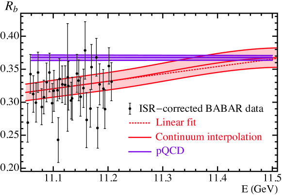
Refer to caption
Figure 9: Comparison of ISR-corrected BABAR data in the continuum region (black dots with error bars) with pQCD (purple band). The red band shows our reconstruction of the continuum, which includes a linear fit to the BaBar data, patched to the pQCD prediction in a smooth way using a cubic polynomial in the energy.

The perturbative QCD theoretical expression which we use to determine this contribution includes the non-singlet massless quark cross section supplemented with bottom mass corrections up to O(m¯b 4/s2O(\overline{m}_{b}^{\,4}/s^{2}).999We note that the double massive fermion bubble contribution to Rbbsubscript𝑅𝑏𝑏R_{bb} in Eq. (6.3) includes both virtual and real radiation terms in the large energy expansion. However, when this formula is used to compare pQCD to the existing BABAR data, below the four-bottom-quarks threshold, the real radiation should be excluded. We have checked that this inconsistency has an effect below 0.10.10.1%. It takes into account only contributions from the electromagnetic current coupled to the bottom quark. It reads: Bernreuther:1981sp ; Gorishnii:1986pz ; Chetyrkin:1993hi ; Chetyrkin:1994ex ; Chetyrkin:2000zk 101010The authors of Ref. Chetyrkin:2010ic use the pole mass instead of the MS¯¯MS\overline{\rm MS}, and include αs4superscriptsubscript𝛼𝑠4\alpha_{s}^{4} and QED corrections. This explains some numerical differences in the analyses.

Rbb¯th(s)=NcQb2Rns(s,m¯b 2(s),nf=5,αs(nf=5)(s)),R^{\rm{th}}_{b\bar{b}}(s)=N_{c}\,Q_{b}^{2}\,R^{\rm{ns}}(s,\overline{m}^{\,2}_{b}(\sqrt{s}),n_{f}=5,\alpha_{s}^{(n_{f}=5)}(\sqrt{s}))\,, (31)

where

Rns(s,m¯b 2(μ),nf=5,αs(nf=5)(μ),μ)\displaystyle R^{\rm{ns}}(s,\overline{m}^{\,2}_{b}(\mu),n_{f}=5,\alpha_{s}^{(n_{f}=5)}(\mu),\mu)
=1+αsπ+(αsπ)2(1.409231.91667Ls)+(αsπ)3( 12.76717.81872Ls+3.67361Ls2)absent1subscript𝛼𝑠𝜋superscriptsubscript𝛼𝑠𝜋21.409231.91667subscript𝐿𝑠superscriptsubscript𝛼𝑠𝜋312.76717.81872subscript𝐿𝑠3.67361superscriptsubscript𝐿𝑠2\displaystyle=1+\frac{\alpha_{s}}{\pi}+\Big{(}\frac{\alpha_{s}}{\pi}\Big{)}^{2}(1.40923-1.91667\,L_{s})+\Big{(}\frac{\alpha_{s}}{\pi}\Big{)}^{3}(-\,12.7671-7.81872\,L_{s}+3.67361\,L_{s}^{2}\,)
+m¯b 2(μ)s[12αsπ+(αsπ)2(104.83347Ls)+(αsπ)3(541.753724.861Ls+137.083Ls2)]subscriptsuperscript¯𝑚2𝑏𝜇𝑠delimited-[]12subscript𝛼𝑠𝜋superscriptsubscript𝛼𝑠𝜋2104.83347subscript𝐿𝑠superscriptsubscript𝛼𝑠𝜋3541.753724.861subscript𝐿𝑠137.083superscriptsubscript𝐿𝑠2\displaystyle+\,\frac{\overline{m}^{\,2}_{b}(\mu)}{s}\Big{[}12\frac{\alpha_{s}}{\pi}+\Big{(}\frac{\alpha_{s}}{\pi}\Big{)}^{2}(104.833-47\,L_{s})+\Big{(}\frac{\alpha_{s}}{\pi}\Big{)}^{3}(541.753-724.861\,L_{s}+137.083\,L_{s}^{2}\,)\Big{]}
+m¯b4(μ)s2[6+(αsπ)( 22+24Ls)+(αsπ)2(139.0144.83333Lm+214.5Ls71Ls2)\displaystyle+\,\frac{\overline{m}_{b}^{\!4}(\mu)}{s^{2}}\Big{[}-6+\Big{(}\frac{\alpha_{s}}{\pi}\Big{)}(-\,22+24\,L_{s})+\Big{(}\frac{\alpha_{s}}{\pi}\Big{)}^{2}(139.014-4.83333\,L_{m}+214.5\,L_{s}-71\,L_{s}^{2}\,)
+(αsπ)3(3545.81158.311Lm+9.66667Lm2538.813Ls+37.8611LmLs\displaystyle+\Big{(}\frac{\alpha_{s}}{\pi}\Big{)}^{3}\ (3545.81-158.311\,L_{m}+9.66667\,L_{m}^{2}-538.813\,L_{s}+37.8611\,L_{m}\,L_{s}
 1037.79Ls2+185.389Ls3)],\displaystyle-\,1037.79\,L_{s}^{2}+185.389\,L_{s}^{3}\,)\Big{]}\,, (32)

with

Lsln(sμ2),Lmln(m¯b 2(μ)s),αs=αs(nf=5)(μ).formulae-sequencesubscript𝐿𝑠𝑠superscript𝜇2formulae-sequencesubscript𝐿𝑚subscriptsuperscript¯𝑚2𝑏𝜇𝑠subscript𝛼𝑠superscriptsubscript𝛼𝑠subscript𝑛𝑓5𝜇L_{s}\equiv\ln\Big{(}\frac{s}{\mu^{2}}\Big{)},\quad L_{m}\equiv\ln\Big{(}\frac{\overline{m}^{\,2}_{b}(\mu)}{s}\Big{)}\,,\quad\alpha_{s}=\alpha_{s}^{(n_{f}=5)}(\mu)\,. (33)

We use the initial conditions m¯b(m¯b)=4.2GeVsubscript¯𝑚𝑏subscript¯𝑚𝑏4.2GeV\overline{m}_{b}(\overline{m}_{b})=4.2\,\rm{GeV} and αs(mZ)=0.118subscript𝛼𝑠subscript𝑚𝑍0.118\alpha_{s}(m_{Z})=0.118.

Therefore, for the continuum region we use the following expression,

MnpQCD=subscriptsuperscript𝑀pQCD𝑛absent\displaystyle M^{\rm pQCD}_{n}= s0s1dsRbbcubic(s)sn+1[1+γ0.04(mZ2s)+0.003(ss0)mZ2s0]superscriptsubscriptsubscript𝑠0subscript𝑠1differential-d𝑠subscriptsuperscript𝑅cubic𝑏𝑏𝑠superscript𝑠𝑛1delimited-[]1superscript𝛾0.04superscriptsubscript𝑚𝑍2𝑠0.003𝑠subscript𝑠0superscriptsubscript𝑚𝑍2subscript𝑠0\displaystyle\int_{s_{0}}^{s_{1}}{\rm d}s\,\frac{R^{\rm{cubic}}_{bb}(s)}{s^{n+1}}\bigg{[}1+\gamma^{\prime}\dfrac{0.04(m_{Z}^{2}-s)+0.003(s-s_{0})}{m_{Z}^{2}-s_{0}}\bigg{]} (34)
+s1mZ2dsRbbth(s)sn+1[1+γ0.04(mZ2s)+0.003(ss0)mZ2s0]superscriptsubscriptsubscript𝑠1superscriptsubscript𝑚𝑍2differential-d𝑠subscriptsuperscript𝑅th𝑏𝑏𝑠superscript𝑠𝑛1delimited-[]1superscript𝛾0.04superscriptsubscript𝑚𝑍2𝑠0.003𝑠subscript𝑠0superscriptsubscript𝑚𝑍2subscript𝑠0\displaystyle+\int_{s_{1}}^{m_{Z}^{2}}{\rm d}s\,\frac{R^{\rm{th}}_{bb}(s)}{s^{n+1}}\bigg{[}1+\gamma^{\prime}\dfrac{0.04(m_{Z}^{2}-s)+0.003(s-s_{0})}{m_{Z}^{2}-s_{0}}\bigg{]}
+(1+0.003γ)mZ2dsRbbth(s)sn+1,γ=0±1,10.003superscript𝛾superscriptsubscriptsuperscriptsubscript𝑚𝑍2differential-d𝑠subscriptsuperscript𝑅th𝑏𝑏𝑠superscript𝑠𝑛1superscript𝛾plus-or-minus01\displaystyle+(1+0.003\,\gamma^{\prime})\int_{m_{Z}^{2}}^{\infty}{\rm d}s\,\frac{R^{\rm{th}}_{bb}(s)}{s^{n+1}}\,,\qquad\gamma^{\prime}=0\pm 1\,,

with s0=(11.2062GeV)2subscript𝑠0superscript11.2062GeV2s_{0}=(11.2062\,{\rm GeV})^{2}, s1=(11.52GeV)2subscript𝑠1superscript11.52GeV2s_{1}=(11.52\,{\rm GeV})^{2} and Rbbcubicsubscriptsuperscript𝑅cubic𝑏𝑏R^{\rm{cubic}}_{bb} is a cubic function that smoothly interpolates between the linear fit to BaBar data and pQCD. Here γsuperscript𝛾\gamma^{\prime} is the auxiliary variable used to parametrize our uncertainty, which we consider as 100%percent100100\% correlated among the various moments. The related entries of the correlation matrix are trivially computed as

CnnpQCD=MnpQCDγMnpQCDγ.superscriptsubscript𝐶𝑛superscript𝑛pQCDsubscriptsuperscript𝑀pQCD𝑛superscript𝛾subscriptsuperscript𝑀pQCDsuperscript𝑛superscript𝛾C_{nn^{\prime}}^{\rm{pQCD}}=\frac{\partial M^{\rm{pQCD}}_{n}}{\partial\gamma^{\prime}}\ \frac{\partial M^{\rm{pQCD}}_{n^{\prime}}}{\partial\gamma^{\prime}}\,. (35)

6.4 Final Results for the Experimental Moments

n Resonances 10.6211.206210.6211.206210.62-11.2062 11.206211.206211.2062-\infty Total
111 1.394(12|22)1.394conditional12221.394(12|22) 0.270(2|9)0.270conditional290.270(2|9) 2.862(0|108)2.862conditional01082.862(0|108) 4.526(12|111)4.526conditional121114.526(12|111)
222 1.459(12|22)1.459conditional12221.459(12|22) 0.226(1|8)0.226conditional180.226(1|8) 1.148(0|45)1.148conditional0451.148(0|45) 2.834(12|51)2.834conditional12512.834(12|51)
333 1.538(12|22)1.538conditional12221.538(12|22) 0.190(1|7)0.190conditional170.190(1|7) 0.611(0|24)0.611conditional0240.611(0|24) 2.338(12|34)2.338conditional12342.338(12|34)
444 1.630(13|22)1.630conditional13221.630(13|22) 0.159(1|6)0.159conditional160.159(1|6) 0.365(0|15)0.365conditional0150.365(0|15) 2.154(13|27)2.154conditional13272.154(13|27)
Table 3: Results for our computations of the experimental moments. The second column collects the contribution from the first four ΥΥ\Upsilon resonances (using the narrow width approximation). The third to fifth columns show the contributions from the threshold (using ISR-corrected BABAR data) and continuum (using an interpolation between a linear fit to the BaBar data with highest energy and pQCD as a model for the lack of data) regions, and the total moment determinations, respectively. The two numbers quoted in parentheses correspond to the uncorrelated and correlated experimental uncertainties, respectively. All numbers are given in units of 10(2n+1)GeV2nsuperscript102𝑛1superscriptGeV2n10^{-(2n+1)}\,\rm{GeV}^{-2n}.

The full result for the experimental moments is obtained by summing up all the portions described before,

Mnexp=Mnres+Mnthr+MnpQCD.subscriptsuperscript𝑀exp𝑛subscriptsuperscript𝑀res𝑛subscriptsuperscript𝑀thr𝑛subscriptsuperscript𝑀pQCD𝑛M^{\rm exp}_{n}=M^{\rm res}_{n}+M^{\rm thr}_{n}+M^{\rm pQCD}_{n}\,. (36)

We determine two correlation matrices among the first four moments. One of them comes from the various uncorrelated uncertainties, whereas the other encodes the systematic uncertainties. We denote them as the correlated and uncorrelated correlation matrices, respectively. These are computed by summing up the respective individual matrices from each region, and in the same way as we did for our charm analysis Dehnadi:2011gc , we assume there is no region-to-region correlation. We find:

Cucexp=(0.00020.00020.00020.00020.00020.00020.00020.00020.00020.00020.00020.00020.00020.00020.00020.0002),Ccorexp=(0.01220.00550.00320.00210.00550.00260.00170.00120.00320.00170.00110.00090.00210.00120.00090.0007),formulae-sequencesubscriptsuperscript𝐶expuc0.00020.00020.00020.00020.00020.00020.00020.00020.00020.00020.00020.00020.00020.00020.00020.0002subscriptsuperscript𝐶expcor0.01220.00550.00320.00210.00550.00260.00170.00120.00320.00170.00110.00090.00210.00120.00090.0007\!\!\!\!C^{\rm exp}_{\rm uc}=\left(\begin{array}[]{cccc}0.0002&0.0002&0.0002&0.0002\\ 0.0002&0.0002&0.0002&0.0002\\ 0.0002&0.0002&0.0002&0.0002\\ 0.0002&0.0002&0.0002&0.0002\\ \end{array}\right)\!,\,C^{\rm exp}_{\rm cor}=\left(\begin{array}[]{cccc}0.0122&0.0055&0.0032&0.0021\\ 0.0055&0.0026&0.0017&0.0012\\ 0.0032&0.0017&0.0011&0.0009\\ 0.0021&0.0012&0.0009&0.0007\\ \end{array}\right)\!, (37)

where the (n,m)𝑛𝑚(n,m) entry of each matrix is given in units of 102(n+m+1)GeV2(n+m)superscript102𝑛𝑚1superscriptGeV2nm10^{-2(n+m+1)}\,\rm{GeV}^{-2(n+m)} , and the total correlation matrix is the sum of Cucexpsubscriptsuperscript𝐶expucC^{\rm exp}_{\rm uc} and Ccorexpsubscriptsuperscript𝐶expcorC^{\rm exp}_{\rm cor}. The contribution of each region to the final experimental moments and the corresponding uncertainties are presented in Table 3.

7 Comparison to other Determinations of the Experimental Moments

In this section we compare our result for the experimental moments for the bottom vector current correlator with previous determinations. These are collected in Table 4.111111In the case of Ref. Corcella:2002uu , we reconstruct the experimental moments from their Table 3, where the moments are split in several different contributions. For the reconstructed uncertainty, we take one half of the error of the narrow resonances correlated to each other, and the other half as uncorrelated. The errors from patches where theory input is used are taken as fully correlated to one another. The total narrow-resonance error, and the total “theory-patch” error are added in quadrature to get the final uncertainty. The most relevant comparison is between the second and third columns, where the most recent data on the narrow resonances and the BABAR continuum data are used. For the contributions from the narrow resonances we have a perfect agreement with Chetyrkin:2009fv , although slightly larger errors. For the threshold region our results are slightly smaller, and our uncertainties are almost identical; however, this is not a one-to-one comparison, since our integration region is slightly smaller. Indeed if we consider their energy range we agree with their numbers almost perfectly. The main difference between these two determinations is the estimate of the uncertainties coming from the continuum region, where the pQCD prediction for the Rbsubscript𝑅𝑏R_{b}-ratio is employed. Whereas we adopt the more conservative approach described in Sec. 6.3, Ref. Chetyrkin:2009fv employs only the perturbative uncertainties related to the purple band in Fig. 9. In Ref. Chetyrkin:2010ic the same collaboration presents a more critical analysis of their errors. In particular they observe that the last experimental measurement of BABAR, after being corrected for ISR, disagrees with the pQCD prediction at the 20%percent2020\% level (way outside the corresponding uncertainties).121212From our own computation of the ISR-corrected Rbsubscript𝑅𝑏R_{b}-ratio, we only observe a 10%percent1010\% deviation between the last data point and the pQCD prediction, see Fig. 9. To resolve this discrepancy they assume two possible scenarios: a) pQCD starts being reliable at energies above 131313 GeV (therefore the authors interpolate between the last experimental point and pQCD at 131313 GeV); b) BABAR systematic errors have been underestimated (therefore the central values of the experimental measurements are rescaled by a factor of 1.211.211.21). Ref. Chetyrkin:2010ic quotes the values of the experimental moments and the resulting values for the bottom mass for these two scenarios. Since the effect of these differences of the two bottom masses obtained from M2Vsuperscriptsubscript𝑀2𝑉M_{2}^{V} is only slightly larger than the size of the other uncertainties (that is, the uncertainties of the theoretical moments plus the other experimental errors) added quadratically, it is argued that this issue can be ignored. We disagree with this argument, since the issue constitutes an independent source of uncertainty not covered by the other errors and, in particular, being unrelated to uncertainties in the theoretical moments. Therefore this shift must be taken as an additional source of error on the experimental moments (and indeed would then dominate the corresponding total error). The additional error (to be added in quadrature to the one in round brackets) is quoted in square brackets in the third column of Table 4. It amounts to an additional error of 30,18,1130181130,18,11 and 777 MeV for m¯b(m¯b)subscript¯𝑚𝑏subscript¯𝑚𝑏\overline{m}_{b}(\overline{m}_{b}) extracted from moments M1Vsuperscriptsubscript𝑀1𝑉M_{1}^{V} to M4Vsuperscriptsubscript𝑀4𝑉M_{4}^{V}, respectively.

Refs. Kuhn:2007vp ; Boughezal:2006px ; Corcella:2002uu have used the older CLEO and CUSB experimental measurements, resulting in relatively large uncertainties. In Ref. Kuhn:2007vp the CLEO measurements are divided by a factor of 1.281.281.28, and an error of 10%percent1010\% is assigned. It is argued that this procedure is necessary to reconcile old and new CLEO measurements, as well as to improve the agreement with pQCD predictions. Ref. Corcella:2002uu uses values for the ΥΥ\Upsilon-states electronic partial widths given by the PDG 2002, which have larger uncertainties. This makes their determination of the experimental moments rather imprecise.

Concerning the continuum region where no measurements exist, while some previous analyses have taken a less conservative approach than ours, in Ref. Beneke:2014pta a much more conservative approach is adopted. In this region they consider the Rbsubscript𝑅𝑏R_{b}-ratio as constant with a 66%percent6666\% uncertainty. In Ref. Corcella:2002uu also a more conservative approach is adopted. Between 11.111.111.1 and 121212 GeV 𝒪(αs2)𝒪superscriptsubscript𝛼𝑠2\mathcal{O}(\alpha_{s}^{2}) pQCD errors are used, which are larger than 101010%; for energies above 121212 GeV a global 10%percent1010\% correlated error is assigned.

n𝑛n This work Chetyrkin et al. ’09 Chetyrkin:2009fv Kuhn et al. ’07 Kuhn:2007vp Corcella et al. ’03 Corcella:2002uu
111 4.526(12|111)4.526conditional121114.526(12|111) 4.592(31)[67]4.59231delimited-[]674.592(31)[67] 4.601(43)4.601434.601(43) 4.46(17)4.46174.46(17)
222 2.834(12|51)2.834conditional12512.834(12|51) 2.872(28)[51]2.87228delimited-[]512.872(28)[51] 2.881(37)2.881372.881(37) 2.76(15)2.76152.76(15)
333 2.338(12|34)2.338conditional12342.338(12|34) 2.362(26)[40]2.36226delimited-[]402.362(26)[40] 2.370(34)2.370342.370(34) 2.26(13)2.26132.26(13)
444 2.154(13|27)2.154conditional13272.154(13|27) 2.170(26)[35]2.17026delimited-[]352.170(26)[35] 2.178(32)2.178322.178(32) 2.08(12)2.08122.08(12)
Table 4: Comparison of our results for the experimental moments of the bottom vector correlator (2nd column) to previous determinations (3rd to 5th columns). The 2nd and 3rd columns use BABAR data from Ref. :2008hx , while 4th and 5th use older data from Refs. Besson:1984bd ; Ammar:1997sk . The 3rd and 4th columns use perturbative uncertainties in the continuum region, while 2nd and 5th use a more conservative estimate based on the agreement of data and pQCD. In the 3rd column, we quote in square brackets our own estimate of an additional systematic error from the considerations made in Ref. Chetyrkin:2010ic . All numbers are given in units of 10(2n+1)GeV2nsuperscript102𝑛1superscriptGeV2n10^{-(2n+1)}\,\rm{GeV}^{-2n}.
Refer to caption
Refer to caption
Refer to caption
Refer to caption
Figure 10: Comparison of various determinations of the experimental moments for the bottom vector correlator. Results in blue correspond to analyses of the same collaboration. The green result and the determination at the top do not use the new BABAR results.

8 Computation of the Experimental Values for the Ratios of Moments

Once the experimental values for the moments of the vector and pseudoscalar correlators have been computed, it is in principle a straightforward exercise to calculate ratios of them. The central value is obtained by simply taking the ratio of the corresponding central values. To obtain the uncertainties (or more generally, the correlation matrix among the different ratios of moments), one needs to have access to the complete correlation matrix among the moments. Our computation in Ref. Dehnadi:2011gc [see Eqs. (3.21) and (3.22)] for the charm experimental moments, and the procedure presented in Sec. 6 [see Eq. (37)] to determine the bottom experimental moments, yield the two desired correlation matrices, for statistical and systematical correlations. For the pseudoscalar moments the information on correlations is not provided in Ref. Allison:2008xk . Therefore we make the simplest possible assumption, which is that the moments are fully uncorrelated. This will most certainly overestimate the uncertainties for the ratios of moments, but given that we are anyway dominated by perturbative uncertainties, our approach appears justified. We collect our results for the computation of the ratios of experimental moments in Table. 5. Readers interested in the full correlation matrix among them can send a request to the authors.

n𝑛n Vector nf=4subscript𝑛𝑓4n_{f}=4 Vector nf=5subscript𝑛𝑓5n_{f}=5 Pseudoscalar nf=4subscript𝑛𝑓4n_{f}=4
111 6.969(32|59)6.969conditional32596.969(32|59) 6.262(10|53)6.262conditional10536.262(10|53) 0.971(32)0.971320.971(32)
222 8.807(23|26)8.807conditional23268.807(23|26) 8.251(09|48)8.251conditional09488.251(09|48) 1.048(53)1.048531.048(53)
333 9.547(14|13)9.547conditional14139.547(14|13) 9.212(08|35)9.212conditional08359.212(08|35) 1.092(77)1.092771.092(77)
Table 5: Ratios of experimental moments for the vector correlator with 444 and 555 flavors (second and third column, respectively), and for the pseudoscalar correlator with 444 flavors (fourth column). For the vector current, the first error in parenthesis corresponds to the statistical uncertainty, whereas the second corresponds to the systematic one. For the pseudoscalar correlator we only quote the lattice error. Moments given in units of 102superscript10210^{-2} GeV-2, 103superscript10310^{-3} GeV-2 and, 101superscript10110^{-1} GeV-2 for the second, third, and fourth column, respectively.

9 Results

In this section we present the final results for our analyses at 𝒪(αs3)𝒪superscriptsubscript𝛼𝑠3\mathcal{O}(\alpha_{s}^{3}). We take method (c) (linearized iterative expansion) as our default expansion. For the estimate of the perturbative uncertainty, we perform double scale variation in the ranges m¯c(m¯c)μα,μm4formulae-sequencesubscript¯𝑚𝑐subscript¯𝑚𝑐subscript𝜇𝛼subscript𝜇𝑚4\overline{m}_{c}(\overline{m}_{c})\leq\mu_{\alpha},\mu_{m}\leq 4 GeV for charm (either correlator), and m¯b(m¯b)μα,μm15formulae-sequencesubscript¯𝑚𝑏subscript¯𝑚𝑏subscript𝜇𝛼subscript𝜇𝑚15\overline{m}_{b}(\overline{m}_{b})\leq\mu_{\alpha},\mu_{m}\leq 15 GeV for bottom, and we discard 3% of the series with the worst convergence (that is, with highest values of the Vcsubscript𝑉𝑐V_{c} convergence parameter). For the charm mass determinations (either vector or pseudoscalar correlator) we use the first moment as our default, given that it is theoretically more reliable than the higher moments. For the analysis of the bottom mass from regular moments, we use M2Vsuperscriptsubscript𝑀2𝑉M_{2}^{V} as our default, since it is less afflicted by systematic experimental errors than the first moment, and is nevertheless theoretically sound. For the charm and the bottom mass analyses we also examine the ratio of the second over the first moment as a cross check and validation of the results from regular moments. The results for the experimental moments are collected in: the last column of Table 9 in Ref. Dehnadi:2011gc (charm vector correlator regular moments); the last column of Table 3 (bottom vector correlator regular moments); Table 1 (lattice regular moments); and Table 5 (all ratios of moments).

We also analyzed higher (and also lower for the case of bottom) moments and ratios of moments for all correlator and quark species. Since, as already discussed, fixed-order and contour-improved higher moments are particularly afflicted by their nonlinear dependence on the quark mass, we only consider the linearized and iterative methods for this analysis. In any case, since higher moments have a larger sensitivity to infrared effects and are therefore theoretically less sound, the analysis involving higher moments mainly aims at providing cross checks. The results are collected in a graphical form in Fig. 11, and the numerical results can be obtained from the authors upon request.
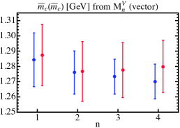
Refer to caption
Refer to caption
Refer to caption
Refer to caption
Refer to caption
Refer to caption
Figure 11: Charm and bottom quark mass determinations for different moments (upper row) or ratios of moments (lower row), for the linearized (in blue) and iterative (in red) methods. Panels (a), (b) [(e), (f)] show the results for the charm mass from moments [ratios of moments] of the vector and pseudoscalar correlator, respectively. Panels (c) and (g) show the results for the bottom mass from the vector correlator, for moments and ratios of moments, respectively.

Our final determinations include nonperturbative effects through the gluon condensate including its Wilson coefficients at order 𝒪(αs)𝒪subscript𝛼𝑠\mathcal{O}(\alpha_{s}). Furthermore, we assign as a conservative estimate of the nonperturbative uncertainty twice the shift caused by including the gluon condensate. In any case, this error is very small, particularly for the bottom mass determination. One source of uncertainty which we have not discussed so far is that coming from the strong coupling constant. Although the world average αs(mZ)=0.1185±0.006subscript𝛼𝑠subscript𝑚𝑍plus-or-minus0.11850.006\alpha_{s}(m_{Z})=0.1185\pm 0.006 has a very small error, see Ref. Agashe:2014kda , one cannot ignore the fact that it is fairly dominated by lattice determinations, e.g. Chakraborty:2014aca . Furthermore, there are other precise determinations with lower central values and in disagreement with the world average from event-shapes Abbate:2010xh ; Abbate:2012jh ; Gehrmann:2012sc ; Hoang:2015hka and DIS Alekhin:2012ig . A review on recent αssubscript𝛼𝑠\alpha_{s} determinations can be found in Refs. Bethke:2011tr ; Bethke:2012jm ; Pich:2013sqa . Therefore, in analogy with Ref. Dehnadi:2011gc , we perform our analyses for several values of αs(mZ)subscript𝛼𝑠subscript𝑚𝑍\alpha_{s}(m_{Z}) between 0.1130.1130.113 and 0.1190.1190.119, and provide the central values and perturbative errors as (approximate) linear functions of αs(mZ)subscript𝛼𝑠subscript𝑚𝑍\alpha_{s}(m_{Z}). The other uncertainties are essentially αssubscript𝛼𝑠\alpha_{s}-independent, so we just provide the average. We also quote quark mass results for αssubscript𝛼𝑠\alpha_{s} taken from the world average:

αs(mZ)=0.1185±0.0021,subscript𝛼𝑠subscript𝑚𝑍plus-or-minus0.11850.0021\alpha_{s}(m_{Z})=0.1185\pm 0.0021\,, (38)

where we adopt an uncertainty 3.53.53.5 times larger than the current world average Agashe:2014kda . We note that in Ref. Dehnadi:2011gc we have taken αs(mZ)=0.1184±0.0021subscript𝛼𝑠subscript𝑚𝑍plus-or-minus0.11840.0021\alpha_{s}(m_{Z})=0.1184\pm 0.0021 as an input which causes only tiny sub-MeV differences in the quark masses. We refrain ourselves from presenting the αssubscript𝛼𝑠\alpha_{s} dependence of the higher-moment result, which the reader can get from the authors upon request.

For the numerical analyses that we carry out in this article we have created two completely independent codes: one using Mathematica mathematica and another using Fortran gfortran , which is much faster and suitable for parallelized runs on computer clusters. The two codes agree for the extracted quark masses at the level of 111\,eV.

9.1 Results for the Charm Mass from the Vector Correlator
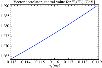
Refer to caption
Refer to caption
Refer to caption
Refer to caption
Figure 12: Dependence on αs(mZ)subscript𝛼𝑠subscript𝑚𝑍\alpha_{s}(m_{Z}) of the central values of m¯c(m¯c)subscript¯𝑚𝑐subscript¯𝑚𝑐{\overline{m}_{c}}({\overline{m}_{c}}) and the corresponding perturbative (red), statistical (orange), systematical (blue) and nonperturbative uncertainties (green), for the analysis of the first moment [panels (a) and (b)] and the ratio of the second over the first moment, [panels (c) and (d)], corresponding to the vector correlator.

For the analysis using the first moment of the charm vector correlator we use the experimental value quoted in Eq. (4.1) of Ref. Dehnadi:2011gc : M1V,exp=(0.2121± 0.0020stat± 0.0030syst)GeV2superscriptsubscript𝑀1𝑉expplus-or-minus0.2121subscript0.0020statsubscript0.0030systsuperscriptGeV2M_{1}^{V,\,\rm exp}=(0.2121\,\pm\,0.0020_{\rm stat}\,\pm\,0.0030_{\rm syst})\,{\rm GeV}^{-2}. The outcome of this analysis, and one of the main results of this paper, is:

m¯c(m¯c)=subscript¯𝑚𝑐subscript¯𝑚𝑐absent\displaystyle\overline{m}_{c}(\overline{m}_{c})=  1.288±(0.006)stat±(0.009)syst±(0.014)pertplus-or-minus1.288subscript0.006statsubscript0.009systsubscript0.014pert\displaystyle\,1.288\,\pm\,(0.006)_{\rm stat}\,\pm\,(0.009)_{\rm syst}\,\pm\,(0.014)_{\rm pert} (39)
±(0.010)αs±(0.002)GGGeV,plus-or-minusplus-or-minussubscript0.010subscript𝛼𝑠subscript0.002delimited-⟨⟩𝐺𝐺GeV\displaystyle\,\pm\,(0.010)_{\alpha_{s}}\,\pm\,(0.002)_{\langle GG\rangle}\,{\rm GeV}\,,

where the quoted errors are (from left to right) experimental uncorrelated, experimental correlated, peturbative, due to the uncertainty in αssubscript𝛼𝑠\alpha_{s} as given in Eq. (38), and nonperturbative. If we adopt the correlated scale variation 2GeVμα=μm42GeVsubscript𝜇𝛼subscript𝜇𝑚42\,{\rm GeV}\leq\mu_{\alpha}=\mu_{m}\leq 4 GeV, we obtain for method (c) 1.297±(0.005)pertplus-or-minus1.297subscript0.005pert1.297\,\pm\,(0.005)_{\rm pert}, with the other errors essentially unchanged. For method (a) we would get 1.290±(0.0007)pertplus-or-minus1.290subscript0.0007pert1.290\,\pm\,(0.0007)_{\rm pert}, with a scale variation even smaller than the nonperturbative uncertainty, and 202020 times smaller than our perturbative error estimate with double scale variation [333 times for method (c)]. The dependence on αs(mZ)subscript𝛼𝑠subscript𝑚𝑍\alpha_{s}(m_{Z}) is shown graphically in Figs. 12 and 12, and analytically the result reads:

m¯c(m¯c)subscript¯𝑚𝑐subscript¯𝑚𝑐\displaystyle\overline{m}_{c}(\overline{m}_{c}) =\displaystyle= (1.288+4.40×[αs(mZ)0.1185])±(0.006)stat±(0.009)systplus-or-minus1.2884.40delimited-[]subscript𝛼𝑠subscript𝑚𝑍0.1185subscript0.006statsubscript0.009syst\displaystyle(1.288+4.40\times[\alpha_{s}(m_{Z})-0.1185])\,\pm\,(0.006)_{\rm stat}\,\pm\,(0.009)_{\rm syst}
±(0.014+0.95×[αs(mZ)0.1185])pert±(0.002)GG.plus-or-minusplus-or-minussubscript0.0140.95delimited-[]subscript𝛼𝑠subscript𝑚𝑍0.1185pertsubscript0.002delimited-⟨⟩𝐺𝐺\displaystyle\,\pm\,(0.014+0.95\times[\alpha_{s}(m_{Z})-0.1185])_{\rm pert}\,\pm\,(0.002)_{\langle GG\rangle}\,.

Eqs. (39) and (9.1) supersede the results given in Eqs. (4.5) and (4.2) of Ref. Dehnadi:2011gc , respectively.

For the ratio of the second over the first moment of the vector correlator we use as the experimental input R1V,exp=(6.969± 0.032stat± 0.059syst)×102superscriptsubscript𝑅1𝑉expplus-or-minus6.969subscript0.032statsubscript0.059systsuperscript102R_{1}^{V,\,\rm exp}=(6.969\,\pm\,0.032_{\rm stat}\,\pm\,0.059_{\rm syst})\times 10^{-2} GeV-2, which yields the following result for the charm mass:

m¯c(m¯c)=subscript¯𝑚𝑐subscript¯𝑚𝑐absent\displaystyle\overline{m}_{c}(\overline{m}_{c})=  1.271±(0.003)stat±(0.005)syst±(0.016)pertplus-or-minus1.271subscript0.003statsubscript0.005systsubscript0.016pert\displaystyle\,1.271\,\pm\,(0.003)_{\rm stat}\,\pm\,(0.005)_{\rm syst}\,\pm\,(0.016)_{\rm pert} (41)
±(0.004)αs±(0.004)GGGeV.plus-or-minusplus-or-minussubscript0.004subscript𝛼𝑠subscript0.004delimited-⟨⟩𝐺𝐺GeV\displaystyle\,\pm\,(0.004)_{\alpha_{s}}\,\pm\,(0.004)_{\langle GG\rangle}\,{\rm GeV}\,.

With correlated variation 2GeVμα=μm4GeV2GeVsubscript𝜇𝛼subscript𝜇𝑚4GeV2\,{\rm GeV}\leq\mu_{\alpha}=\mu_{m}\leq 4\,{\rm GeV} we get 1.258±(0.005)pertplus-or-minus1.258subscript0.005pert1.258\,\pm\,(0.005)_{\rm pert} and 1.279±(0.007)pertplus-or-minus1.279subscript0.007pert1.279\,\pm\,(0.007)_{\rm pert} for methods (a) and (c), respectively. In this case the scale variations are a factor of 222 to 333 smaller than our perturbative error estimate.131313Had we taken the fixed-order expansion (a) and correlated scale variation 2GeVμα=μm4GeV2GeVsubscript𝜇𝛼subscript𝜇𝑚4GeV2\,{\rm GeV}\leq\mu_{\alpha}=\mu_{m}\leq 4\,{\rm GeV} as the estimate for the perturbative uncertainty, the result from R1Vsuperscriptsubscript𝑅1𝑉R_{1}^{V} with all errors added quadratically would be 1.258±0.013plus-or-minus1.2580.0131.258\pm 0.013 GeV, whereas the result from M1Vsuperscriptsubscript𝑀1𝑉M_{1}^{V} would read 1.290±0.015plus-or-minus1.2900.0151.290\pm 0.015 GeV. Both results would not be consistent to each other. The αssubscript𝛼𝑠\alpha_{s} dependence, which can be seen in Figs. 12 and 12, has the form:

m¯c(m¯c)subscript¯𝑚𝑐subscript¯𝑚𝑐\displaystyle\overline{m}_{c}(\overline{m}_{c}) =(1.271+1.64×[αs(mZ)0.1185])±(0.003)stat±(0.005)systabsentplus-or-minus1.2711.64delimited-[]subscript𝛼𝑠subscript𝑚𝑍0.1185subscript0.003statsubscript0.005syst\displaystyle=(1.271+1.64\times[\alpha_{s}(m_{Z})-0.1185])\,\pm\,(0.003)_{\rm stat}\,\pm\,(0.005)_{\rm syst} (42)
±(0.016+1.081×[αs(mZ)0.1185])pert±(0.004)GG.plus-or-minusplus-or-minussubscript0.0161.081delimited-[]subscript𝛼𝑠subscript𝑚𝑍0.1185pertsubscript0.004delimited-⟨⟩𝐺𝐺\displaystyle\,\pm\,(0.016+1.081\times[\alpha_{s}(m_{Z})-0.1185])_{\rm pert}\,\pm\,(0.004)_{\langle GG\rangle}\,.

We observe that the central value for the ratios of moments is 171717 MeV smaller than for the first moment analysis, but fully compatible within theoretical uncertainties. Furthermore, the dependence on αssubscript𝛼𝑠\alpha_{s} of the central value obtained from the regular moment analysis is larger, which translates into a corresponding larger error due to the uncertainty in αssubscript𝛼𝑠\alpha_{s}. Both determinations have very similar perturbative uncertainties for any value of αssubscript𝛼𝑠\alpha_{s}. We also see that the charm mass from the ratio of moments has smaller experimental uncertainties, as a result of cancellations between correlated errors. Moreover, the charm mass result from R1Vsuperscriptsubscript𝑅1𝑉R_{1}^{V} has a nonperturbative error twice as large as that from M1Vsuperscriptsubscript𝑀1𝑉M_{1}^{V}. The two charm mass results from the first moment and the moment ratio are compared graphically in Fig. 15.

9.2 Results for the Charm Mass from the Pseudoscalar Correlator
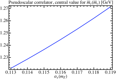
Refer to caption
Refer to caption
Refer to caption
Refer to caption
Figure 13: Dependence on αs(mZ)subscript𝛼𝑠subscript𝑚𝑍\alpha_{s}(m_{Z}) of the central values of m¯c(m¯c)subscript¯𝑚𝑐subscript¯𝑚𝑐{\overline{m}_{c}}({\overline{m}_{c}}) and the corresponding perturbative (red), lattice (blue) and nonperturbative uncertainties (green), for the analysis of the first moment [panels (a) and (b)] and the ratio of the second over the first moment, [panels (c) and (d)], corresponding to the pseudoscalar correlator.

For the analysis of the first moment of the charm pseudoscalar correlator we employ M1P,latt=(0.1402± 0.0020latt)GeV2superscriptsubscript𝑀1𝑃lattplus-or-minus0.1402subscript0.0020lattsuperscriptGeV2M_{1}^{P,\,{\rm latt}}\,=\,(0.1402\,\pm\,0.0020_{\rm latt})\,{\rm GeV}^{-2} Allison:2008xk , which yields the following charm mass determination:

m¯c(m¯c)= 1.267±(0.008)lat±(0.035)pert±(0.019)αs±(0.002)GGGeV.subscript¯𝑚𝑐subscript¯𝑚𝑐plus-or-minus1.267subscript0.008latsubscript0.035pertsubscript0.019subscript𝛼𝑠subscript0.002delimited-⟨⟩𝐺𝐺GeV\displaystyle\overline{m}_{c}(\overline{m}_{c})=\,1.267\,\pm\,(0.008)_{\rm lat}\,\pm\,(0.035)_{\rm pert}\,\pm\,(0.019)_{\alpha_{s}}\,\pm\,(0.002)_{\langle GG\rangle}\,{\rm GeV}\,. (43)

With correlated scale variation 2GeVμα=μm4GeV2GeVsubscript𝜇𝛼subscript𝜇𝑚4GeV2\,{\rm GeV}\leq\mu_{\alpha}=\mu_{m}\leq 4\,{\rm GeV} we obtain the central values 1.2781.2781.278 and 1.2761.2761.276 GeV, for methods (b) and (c), respectively. In both cases the scale variation is 444 MeV, 8 times smaller than our perturbative error estimate with double scale variation. For the αssubscript𝛼𝑠\alpha_{s} dependence, we find

m¯c(m¯c)subscript¯𝑚𝑐subscript¯𝑚𝑐\displaystyle\overline{m}_{c}(\overline{m}_{c}) =(1.267+8.36×[αs(mZ)0.1185])±(0.008)latabsentplus-or-minus1.2678.36delimited-[]subscript𝛼𝑠subscript𝑚𝑍0.1185subscript0.008lat\displaystyle=(1.267+8.36\times[\alpha_{s}(m_{Z})-0.1185])\,\pm\,(0.008)_{\rm lat} (44)
±(0.035+2.38×[αs(mZ)0.1185])pert±(0.002)GG,plus-or-minusplus-or-minussubscript0.0352.38delimited-[]subscript𝛼𝑠subscript𝑚𝑍0.1185pertsubscript0.002delimited-⟨⟩𝐺𝐺\displaystyle\,\pm\,(0.035+2.38\times[\alpha_{s}(m_{Z})-0.1185])_{\rm pert}\,\pm\,(0.002)_{\langle GG\rangle}\,,

which is also displayed in Figs. 13 and 13. As expected, the perturbative error is much larger than for the vector correlator, and has a stronger dependence on αssubscript𝛼𝑠\alpha_{s}. We see that the central value has a much stronger dependence on αssubscript𝛼𝑠\alpha_{s} as well, which again translates into a large error due to the uncertainty in the strong coupling. The central value is 212121 MeV lower than Eq. (39), but fully compatible within errors [see Fig 15]. The nonperturbative uncertainties are identical to the vector current case.

For the ratio of second over the first moment of the pseudoscalar correlator we use R1P,latt=(0.0971± 0.0032latt)superscriptsubscript𝑅1𝑃lattplus-or-minus0.0971subscript0.0032lattR_{1}^{P,\,\rm latt}=(0.0971\,\pm\,0.0032_{\rm latt})\,GeV-2. We find for the charm mass

m¯c(m¯c)= 1.266±(0.020)latt±(0.018)pert±(0.006)αs±(0.002)GGGeV.subscript¯𝑚𝑐subscript¯𝑚𝑐plus-or-minus1.266subscript0.020lattsubscript0.018pertsubscript0.006subscript𝛼𝑠subscript0.002delimited-⟨⟩𝐺𝐺GeV\displaystyle\overline{m}_{c}(\overline{m}_{c})=\,1.266\,\pm\,(0.020)_{\rm latt}\,\pm\,(0.018)_{\rm pert}\,\pm\,(0.006)_{\alpha_{s}}\,\pm\,(0.002)_{\langle GG\rangle}\,{\rm GeV}\,. (45)

Using correlated variation 2GeVμα=μm4GeV2GeVsubscript𝜇𝛼subscript𝜇𝑚4GeV2\,{\rm GeV}\leq\mu_{\alpha}=\mu_{m}\leq 4\,{\rm GeV} one obtains 1.270±(0.007)pertplus-or-minus1.270subscript0.007pert1.270\,\pm\,(0.007)_{\rm pert} and 1.278±(0.003)pertplus-or-minus1.278subscript0.003pert1.278\,\pm\,(0.003)_{\rm pert} for methods (a) and (c), respectively. These scale variations are a factor 333 and 666 smaller than our perturbative error estimate, respectively. The αssubscript𝛼𝑠\alpha_{s} dependence is

m¯c(m¯c)subscript¯𝑚𝑐subscript¯𝑚𝑐\displaystyle\overline{m}_{c}(\overline{m}_{c}) =(1.266+2.31×[αs(mZ)0.1185])±(0.020)lattabsentplus-or-minus1.2662.31delimited-[]subscript𝛼𝑠subscript𝑚𝑍0.1185subscript0.020latt\displaystyle=(1.266+2.31\times[\alpha_{s}(m_{Z})-0.1185])\,\pm\,(0.020)_{\rm latt} (46)
±(0.018+1.25×[αs(mZ)0.1185])pert±(0.002)GG.plus-or-minusplus-or-minussubscript0.0181.25delimited-[]subscript𝛼𝑠subscript𝑚𝑍0.1185pertsubscript0.002delimited-⟨⟩𝐺𝐺\displaystyle\,\pm\,(0.018+1.25\times[\alpha_{s}(m_{Z})-0.1185])_{\rm pert}\,\pm\,(0.002)_{\langle GG\rangle}\,.

The central values for both M1Psuperscriptsubscript𝑀1𝑃M_{1}^{P} and R1Psuperscriptsubscript𝑅1𝑃R_{1}^{P} are almost identical, but their αssubscript𝛼𝑠\alpha_{s} dependence is not: the latter is much smaller (even smaller than for M1Vsuperscriptsubscript𝑀1𝑉M_{1}^{V}, but larger than for R1Vsuperscriptsubscript𝑅1𝑉R_{1}^{V}). Note that the lattice error is larger for the ratio since we made the very conservative assumption that they are fully uncorrelated. This is because the correlation matrix for various lattice moments is unknown. The perturbative error reduces by a factor of two for any value of αssubscript𝛼𝑠\alpha_{s} when using the ratio, but we have checked that this only happens for the iterative expansion. On the other hand, the αssubscript𝛼𝑠\alpha_{s} dependence of the perturbative uncertainty is smaller for the regular moment determination. The nonperturbative errors are identical.

All charm determinations are illustrated graphically in Fig. 15, where in red we show our preferred determination from the first moment of the vector correlator.

9.3 Results for the Bottom Mass from the Vector Correlator
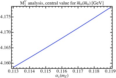
Refer to caption
Refer to caption
Refer to caption
Refer to caption
Figure 14: Dependence on αs(mZ)subscript𝛼𝑠subscript𝑚𝑍\alpha_{s}(m_{Z}) of the central values of m¯b(m¯b)subscript¯𝑚𝑏subscript¯𝑚𝑏{\overline{m}_{b}}({\overline{m}_{b}}) and the corresponding perturbative (red), statistical (orange), systematical (blue) and nonperturbative uncertainties (green), for for the analysis of the second moment [panels (a) and (b)] and the ratio of the second over the the first moment [panels (c) and (d)] of the vector correlator.

For our determination of the bottom quark mass from the second moment of the vector correlator we use for the experimental moment M2V,exp=(2.834± 0.012stat± 0.051syst)×105superscriptsubscript𝑀2𝑉expplus-or-minus2.834subscript0.012statsubscript0.051systsuperscript105M_{2}^{V,\,\rm exp}=(2.834\,\pm\,0.012_{\rm stat}\,\pm\,0.051_{\rm syst})\times 10^{-5} GeV-4, and we obtain

m¯b(m¯b)=subscript¯𝑚𝑏subscript¯𝑚𝑏absent\displaystyle\overline{m}_{b}(\overline{m}_{b})=  4.176±(0.004)stat±(0.019)syst±(0.010)pertplus-or-minus4.176subscript0.004statsubscript0.019systsubscript0.010pert\displaystyle\,4.176\,\pm\,(0.004)_{\rm stat}\,\pm\,(0.019)_{\rm syst}\,\pm\,(0.010)_{\rm pert} (47)
±(0.007)αs±(0.0001)GGGeV.plus-or-minusplus-or-minussubscript0.007subscript𝛼𝑠subscript0.0001delimited-⟨⟩𝐺𝐺GeV\displaystyle\,\pm\,(0.007)_{\alpha_{s}}\,\pm\,(0.0001)_{\langle GG\rangle}\,{\rm GeV}\,.

The perturbative error is 30%percent3030\% smaller than for the charm vector correlator analysis, as a result of the smaller value of αssubscript𝛼𝑠\alpha_{s} at the scales close to the bottom mass. This is consistent with our discussion on the convergence properties of perturbation series for the bottom quark carried out in Sec. 4. The total error is dominated by the experimental systematic uncertainty, which in turn mainly comes from the continuum region where one relies on modeling in the absence of any experimental measurements. The nonperturbative error is completely negligible. This is expected since it is suppressed by two powers of the bottom mass. Using the correlated scale variation 5GeVμα=μm15GeV5GeVsubscript𝜇𝛼subscript𝜇𝑚15GeV5\,{\rm GeV}\leq\mu_{\alpha}=\mu_{m}\leq 15\,{\rm GeV} for methods (a) and (c) we get 4.1784.1784.178 and 4.1824.1824.182 for the central values and scale variations which are 202020 and 333 times smaller, respectively. The αssubscript𝛼𝑠\alpha_{s} dependence reads

m¯b(m¯b)subscript¯𝑚𝑏subscript¯𝑚𝑏\displaystyle\overline{m}_{b}(\overline{m}_{b}) =(4.176+3.22×[αs(mZ)0.1185])±(0.004)stat±(0.019)systabsentplus-or-minus4.1763.22delimited-[]subscript𝛼𝑠subscript𝑚𝑍0.1185subscript0.004statsubscript0.019syst\displaystyle=(4.176+3.22\times[\alpha_{s}(m_{Z})-0.1185])\,\pm\,(0.004)_{\rm stat}\,\pm\,(0.019)_{\rm syst} (48)
±(0.010+0.472×[αs(mZ)0.1185])pert±(0.0001)GG.plus-or-minusplus-or-minussubscript0.0100.472delimited-[]subscript𝛼𝑠subscript𝑚𝑍0.1185pertsubscript0.0001delimited-⟨⟩𝐺𝐺\displaystyle\,\pm\,(0.010+0.472\times[\alpha_{s}(m_{Z})-0.1185])_{\rm pert}\,\pm\,(0.0001)_{\langle GG\rangle}\,.

For the analysis based on the ratio of the second moment over the first, we use R2V,exp=(6.262± 0.010stat± 0.053syst)×103superscriptsubscript𝑅2𝑉expplus-or-minus6.262subscript0.010statsubscript0.053systsuperscript103R_{2}^{V,\,\rm exp}=(6.262\,\pm\,0.010_{\rm stat}\,\pm\,0.053_{\rm syst})\times 10^{-3} GeV-2, and with this value we obtain the bottom mass

m¯b(m¯b)=subscript¯𝑚𝑏subscript¯𝑚𝑏absent\displaystyle\overline{m}_{b}(\overline{m}_{b})=  4.179±(0.003)stat±(0.017)syst±(0.009)pertplus-or-minus4.179subscript0.003statsubscript0.017systsubscript0.009pert\displaystyle\,4.179\,\pm\,(0.003)_{\rm stat}\,\pm\,(0.017)_{\rm syst}\,\pm\,(0.009)_{\rm pert} (49)
±(0.003)αs±(0.0002)GGGeV.plus-or-minusplus-or-minussubscript0.003subscript𝛼𝑠subscript0.0002delimited-⟨⟩𝐺𝐺GeV\displaystyle\,\pm\,(0.003)_{\alpha_{s}}\,\pm\,(0.0002)_{\langle GG\rangle}\,{\rm GeV}\,.

With correlated scale variation 5GeVμα=μm15GeV5GeVsubscript𝜇𝛼subscript𝜇𝑚15GeV5\,{\rm GeV}\leq\mu_{\alpha}=\mu_{m}\leq 15\,{\rm GeV} we obtain 4.175±(0.003)pertplus-or-minus4.175subscript0.003pert4.175\,\pm\,(0.003)_{\rm pert} and 4.182±(0.004)pertplus-or-minus4.182subscript0.004pert4.182\,\pm\,(0.004)_{\rm pert} for methods (a) and (c), respectively. In this case the scale variation is smaller by a factor 333 and 222, respectively. The αssubscript𝛼𝑠\alpha_{s} dependence reads as follows:

m¯b(m¯b)subscript¯𝑚𝑏subscript¯𝑚𝑏\displaystyle\overline{m}_{b}(\overline{m}_{b}) =(4.179+1.199×[αs(mZ)0.1185])±(0.003)stat±(0.017)systabsentplus-or-minus4.1791.199delimited-[]subscript𝛼𝑠subscript𝑚𝑍0.1185subscript0.003statsubscript0.017syst\displaystyle=(4.179+1.199\times[\alpha_{s}(m_{Z})-0.1185])\,\pm\,(0.003)_{\rm stat}\,\pm\,(0.017)_{\rm syst} (50)
±(0.009+0.426×[αs(mZ)0.1185])pert±(0.0002)GG.plus-or-minusplus-or-minussubscript0.0090.426delimited-[]subscript𝛼𝑠subscript𝑚𝑍0.1185pertsubscript0.0002delimited-⟨⟩𝐺𝐺\displaystyle\,\pm\,(0.009+0.426\times[\alpha_{s}(m_{Z})-0.1185])_{\rm pert}\,\pm\,(0.0002)_{\langle GG\rangle}\,.

Although the central value for the ratio analysis is 333 MeV higher, this has no significance given the size of the uncertainties. The dependence of the central value on αssubscript𝛼𝑠\alpha_{s} is three times smaller for the ratio analysis. The perturbative error and its αssubscript𝛼𝑠\alpha_{s} dependence are roughly the same for the ratio and the single moment analysis. Moreover, the two experimental errors are very similar. This is because, even though there is some cancellation of correlated errors in the ratio, a significant part of the huge systematic error of the first moment remains uncanceled.

A graphical illustration of the two bottom mass determinations is shown in Fig. 15. Both combined uncertainties and central values are rather similar, and we adopt the result from the second moment (in red) as our default result.
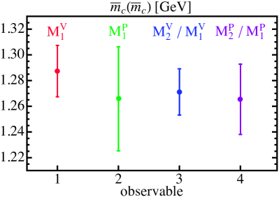
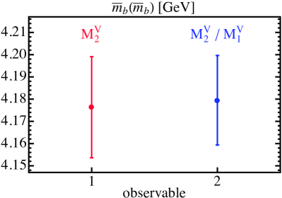
Refer to caption
Refer to caption
Figure 15: Charm (a) [bottom (b)] mass determinations from the first [second] moment of the vector correlator (in red), the first moment of the pseudoscalar correlator (green, charm only), and the ratio of the second over the first moment of the vector (blue) and pseudoscalar correlator (purple, charm only).

10 Comparison to other Determinations

In this section we make a comparison to previous analyses of our updated charm mass determination from the vector correlator, our new results for the charm mass from the pseudoscalar current correlator and of our bottom mass determination. We restrict our discussion to determinations which use QCD sum rules with infinite as well as finite energy range for the vector or pseudoscalar current correlators, and including relativistic and nonrelativistic versions of the sum rules. We do not cover charm mass determinations from DIS or bottom mass determinations from jets (which are in any case rather imprecise), as well as determinations which are based on the mass of bound states (B mesons or quarkonia) or B decays.

In Figs. 16 and 16 we present in a graphical form a compilation of recent sum rule determinations of the charm and bottom masses, respectively. We have labeled them from top to bottom with numbers from 111 to 141414. We note that comparing these results, one has to keep in mind that different analyses in general employed different values and uncertainties for the strong coupling. Only the analyses in Refs. Hoang:2004xm ; Chetyrkin:2009fv ; Bodenstein:2010qx ; Dehnadi:2011gc ; Hoang:2012us and ours have provided the dependence of their results on the value of αs(mZ)subscript𝛼𝑠subscript𝑚𝑍\alpha_{s}(m_{Z}).

10.1 Charm Mass

Let us first focus our attention on the charm mass, Fig. 16. Within each color, determinations are ordered according to publication date. In red (determinations 121212 to 141414) we show the results of our collaboration: 121212 and 131313 for the vector correlator, the former (dashed) corresponding to Ref. Dehnadi:2011gc without trimming procedure, and the latter (solid) corresponding to this work, which includes the trimming procedure. Determinations 121212 to 141414 are the only analyses using uncorrelated scale variation. Determination 666 (gray) Hoang:2004xm sets μm=m¯c(m¯c)subscript𝜇𝑚subscript¯𝑚𝑐subscript¯𝑚𝑐\mu_{m}=\overline{m}_{c}(\overline{m}_{c}), and all the other analyses have set μm=μαsubscript𝜇𝑚subscript𝜇𝛼\mu_{m}=\mu_{\alpha}. Determinations in blue (111 Chakraborty:2014aca , 222 McNeile:2010ji and 333 Allison:2008xk ) were performed by the HPQCD collaboration, which employ method (b) for the pseudoscalar correlator moments used for the mass determination in their lattice analyses. Only 111 to 333 and 141414 use pseudoscalar moments, while all the other analyses use the vector correlator. Among those 777 Bodenstein:2011ma , 888 Chetyrkin:2009fv , 999 Kuhn:2007vp and 101010 Boughezal:2006px use data in the threshold region only up to 4.84.84.8 GeV; analysis 666 uses two patches of data in the threshold region, one from threshold to 4.74.74.7 GeV, and another between 7.27.27.2 and 111111 GeV; analyses 121212 and 131313 use all available data (see Ref. Dehnadi:2011gc for the complete bibliographic information on charm data). The result in 666 uses only 𝒪(αs2)𝒪superscriptsubscript𝛼𝑠2\mathcal{O}(\alpha_{s}^{2}) perturbative input [all the other analyses utilize 𝒪(αs3)𝒪superscriptsubscript𝛼𝑠3\mathcal{O}(\alpha_{s}^{3}) computations] and older information on the narrow resonances, from the PDG 2006. They also study the fixed-order expansion and two methods of contour improvement. In black (888 to 101010) we display results using fixed order analyses at 𝒪(αs3)𝒪superscriptsubscript𝛼𝑠3{\cal O}(\alpha_{s}^{3}) from the Karlsruhe (888 and 999) and Würzburg (101010) collaborations.

Analysis 777 (orange) corresponds to weighted finite-energy sum rules. They employ a kernel which enhances the sensitivity to the charm mass, and at the same time reduces the sensitivity to the continuum region. Green color analyses, collected in 444 Narison:2010cg ; Narison:2011xe and 555 Bodenstein:2010qx , apply other kinds of sum rules. Analysis 555 uses a finite energy sum rule similar to 777, but the kernel makes the sensitivity to the charm mass quite small. On the other hand, the two determinations of 444 use shifted moments, ratios of shifted moments, and exponential sum rules, and consider only the contributions from the first 6 vector resonances in the narrow width approximation, and the pQCD prediction for the continuum. The lower analysis of 444 Narison:2010cg includes contributions from condensates up to dimension 6; the higher Narison:2011xe includes condensates up to dimension 8. In purple (111111 Signer:2008da ) we show the only analysis which uses large-n𝑛n moments for the charm mass fits, employing NRQCD methods to sum up large logs and threshold enhanced perturbative corrections, supplemented with fixed order predictions for the formally power suppressed terms. This analysis uses contributions from narrow resonances, plus a crude model for the threshold and continuum patches, for which a conservative uncertainty is assigned. We note, however, that this analysis might be questioned since perturbative NRQCD is in general not applicable for the charmonium states.

Our new vector correlator result agrees well with the world average, having a similar uncertainty. Our result is fully compatible with the other determinations shown in Fig. 16. As mentioned already before, we disagree with the small perturbative uncertainties related to the scale variations of the vector and/or pseudoscalar moments adopted in analyses 111 to 333 and 777 to 101010.

10.2 Bottom Mass

Let us now turn our attention to the bottom mass results, see Fig. 16. The coloring and chronological conventions are analogous to Fig. 16, and we try to keep a similar ordering. We show three nonrelativistic determinations (111111 Hoang:2012us , 121212 Beneke:2014pta and 131313 Penin:2014zaa ) in purple; 𝒪(αs2)𝒪superscriptsubscript𝛼𝑠2\mathcal{O}(\alpha_{s}^{2}) fixed-order analyses are shown in gray (555 Corcella:2002uu ), black (101010 Erler:2002bu ) and green (444 Bordes:2002ng ); finite energy sum rules also based on fixed-order appear in orange (666 Bodenstein:2012 ) and green (444); there are two lattice analyses in blue, collected in 111 Colquhoun:2014ica ; McNeile:2010ji . Analyses 333, 666, 777 and 111111 to 131313 use the new BABAR data, whereas the others use the older CLEO and CUSB data. Analyses 444 and 111111 include only the contributions of the first six vector resonances. Analyses 444 and 555 use older measurements of the electronic width for the narrow resonances. Analyses 333, 444, 666 to 999 use pQCD in the high-energy spectrum for the experimental moments. The theoretical treatment of the bottom mass analyses in red, gray, black, blue and green are in complete analogy to their charm mass analyses: 333 and 444 for bottom correspond to 444 and 555 for charm, respectively; 111 in bottom corresponds to 111 and 222 for charm.

The upper analysis of 111 Colquhoun:2014ica uses a nonrelativistic lattice action to compute ratios of large-n𝑛n moments, which are later compared to relativistic continuum perturbation theory. Because the continuum computation do not sum up Sommerfeld enhanced terms, this procedure is questionable. The analysis 101010 uses a combination of M6Vsuperscriptsubscript𝑀6𝑉M_{6}^{V} with the infinite momentum transfer moment, both in fixed-order, in order to constrain the continuum region. They only use experimental information on narrow resonances, and model the rest of the spectrum with theory predictions. Finally, they make the following scale choice: μα=μm=m¯b(m¯b)subscript𝜇𝛼subscript𝜇𝑚subscript¯𝑚𝑏subscript¯𝑚𝑏\mu_{\alpha}=\mu_{m}=\overline{m}_{b}(\overline{m}_{b}) and estimate the truncation error from an ansatz for the 𝒪(αs3)𝒪superscriptsubscript𝛼𝑠3\mathcal{O}(\alpha_{s}^{3}) term.141414Ref. Erler:2002bu also makes a determination of the charm mass. We exclude it from our comparison since it is not used in the PDG average. Analyses 111111 and 131313 use large-n𝑛n moments and NRQCD methods for their theoretical moments. Analysis 121212 uses NRQCD fixed-order perturbation theory at N3LO (which accounts for the summation of the Coulomb singularities) and 131313 uses renormalization group improved perturbation theory in the framework of vNRQCD at N2LL order. Both analyses employ low-scale short-distance masses to avoid ambiguities related to the pole mass renormalon. Analysis 121212 also uses N3LO NRQCD fixed-order input, but is incomplete concerning the contributions from the continuum region in the theoretical moments. Moreover, they extract the pole mass which is then converted to the MS¯¯MS{\overline{\rm MS}} scheme.

Our result 141414 is in full agreement with the world average, having a slightly smaller uncertainty. It also agrees with the other analyses shown, with slightly smaller or comparable uncertainties. We disagree with the small perturbative uncertainties related to scale variations quoted in 666 to 101010.

Refer to caption
Refer to caption
Figure 16: Comparison of recent determinations of charm (a) and bottom (b) quark masses from sum rule analyses. Red results correspond to our determination. Black and gray correspond to 𝒪(αs2)𝒪superscriptsubscript𝛼𝑠2\mathcal{O}(\alpha_{s}^{2}) and 𝒪(αs3)𝒪superscriptsubscript𝛼𝑠3\mathcal{O}(\alpha_{s}^{3}) analyses, respectively. Purple results use nonrelativistic sum rules. Orange use weighted finite energy sum rules. Blue results are based on QCD sum rules using lattice simulation results as experimental data. Green labels other kinds of sum rule analyses (FESR, Q2superscript𝑄2Q^{2}-dependent moments, ratios of moments).

11 Conclusions

In this work we have determined the MS¯¯MS\overline{\rm MS} charm and bottom quark masses from quarkonium sum rules in the framework of the OPE, using 𝒪(αs3)𝒪superscriptsubscript𝛼𝑠3\mathcal{O}(\alpha_{s}^{3}) perturbative computations, plus nonperturbative effects from the gluon condensate including its Wilson coefficient at 𝒪(αs)𝒪subscript𝛼𝑠\mathcal{O}(\alpha_{s}). For the determination of the perturbative uncertainties we independently varied the renormalization scales of the strong coupling and the quark masses, in order to account for the variations due to different possible types of αssubscript𝛼𝑠\alpha_{s} expansions, as suggested earlier in Ref. Dehnadi:2011gc .

In order to avoid a possible overestimate of the perturbative uncertainties, coming from the double scale variation in connection with a low scale of αssubscript𝛼𝑠\alpha_{s} and resulting in badly convergent series, we have re-examined the charm mass determination from charmonium sum rules (vector correlator) supplementing the analysis with a convergence test. The convergence test is based on Cauchy’s radical test, which is adapted to the situation in which only a few terms of the series are known, and quantifies the convergence rate of each series by the parameter Vcsubscript𝑉𝑐V_{c}. We find that the distribution of the convergence parameter Vcsubscript𝑉𝑐V_{c} coming from the complete set of series peaks around its mean value, and allows to quantify the overall convergence rate of the set of series for each moment in a meaningful way. This justifies discarding (or “trimming”) series with values of Vcsubscript𝑉𝑐V_{c} much larger than the average. For our analysis we discard 3%percent33\% of the series having the highest Vcsubscript𝑉𝑐V_{c} values, which results in a reduction of the perturbative uncertainty for the MS¯¯MS\overline{\rm MS} charm mass m¯c(m¯c)subscript¯𝑚𝑐subscript¯𝑚𝑐\overline{m}_{c}(\overline{m}_{c}) from 191919 MeV in Dehnadi:2011gc to 141414 MeV (which amounts to 26%), and a small shift of + 55+\,5 MeV in the central value. Our new determination of the charm mass from the first moment (which is theoretically the cleanest) of the vector correlator reads:

m¯c(m¯c)= 1.288±0.020GeV,[VectorCorrelator]subscript¯𝑚𝑐subscript¯𝑚𝑐plus-or-minus1.2880.020GeVdelimited-[]VectorCorrelator\overline{m}_{c}(\overline{m}_{c})=\,1.288\,\pm 0.020\,\rm GeV\,,\qquad{\rm[Vector~{}Correlator]} (51)

where all sources of uncertainty have been added in quadrature. This result supersedes our corresponding earlier result from Ref. Dehnadi:2011gc , which was 1.282± 0.024plus-or-minus1.2820.0241.282\,\pm\,0.024 GeV. This makes it clear that the trimming procedure discards series which produce small values of the charm mass.

We have applied the same method of theory uncertainty estimate to analyze the HPQCD lattice simulation results for the pseudoscalar correlator. Our convergence test signals that the pseudoscalar moments have far worse convergence than the corresponding vector ones. This translates into an uncertainties of 353535 MeV due to the truncation of the perturbative series and the error in αssubscript𝛼𝑠\alpha_{s} (roughly twice as big as for the vector determination). In contrast, using correlated scale variation (e.g. setting the scales in the mass and the strong coupling equal) the scale variation can be smaller by a factor of 888. Our new determination from the first moment (again being the most reliable theoretical prediction) of the pseudoscalar correlator reads m¯c(m¯c)=1.267±0.041subscript¯𝑚𝑐subscript¯𝑚𝑐plus-or-minus1.2670.041\overline{m}_{c}(\overline{m}_{c})=1.267\pm 0.041 GeV, where again all individual errors have been added in quadrature. The combined total error is twice as big as for the vector correlator, and therefore we consider it as a validation of Eq. (51) in connection with the convergence test. The result is in sharp contrast with the analyses carried out by the HPQCD collaboration Allison:2008xk ; McNeile:2010ji ; Chakraborty:2014aca , where perturbative uncertainties of 444 MeV are claimed. We have checked that, as for the vector correlator, for the different possible types of αssubscript𝛼𝑠\alpha_{s}-expansion the correlated variation in general leads to a bad order-by-order convergence of the charm mass determination.

The second important result of this work is the determination of the bottom quark mass from the vector correlator. We have reanalyzed the experimental moments by combining experimental measurements of the first four narrow resonances, the threshold region covered by BABAR, and a theoretical model for the continuum. This theoretical model is an interpolation between a linear fit to the BaBar data points with highest energy and pQCD, to which we assign a 4%percent44\% systematic uncertainty which decreases linearly to reach 0.3%percent0.30.3\% at the Z𝑍Z-pole, and stays constant at 0.3%percent0.30.3\% for higher energies. Our treatment is motivated by the error function yielded by the fit to BaBar data in the energy range between 11.011.011.0 and 11.211.211.2 GeV and the discrepancy between pQCD and experimental measurements at the Z𝑍Z-pole. This results into a large error for the first moment, and therefore we choose the second moment (which is theoretically as clean as the first one for the case of the bottom quark) for our final analysis, giving a total experimental uncertainty of 181818 MeV. Our treatment of the experimental continuum uncertainty is in contrast to Ref. Chetyrkin:2009fv , where instead the very small perturbative QCD uncertainties (less than 111%) are used, claiming an experimental uncertainties of 666 MeV. In the light of the analysis carried out here, supported by the observations made in Ref. Chetyrkin:2010ic , we believe this is not justified. Our convergence test reveals that, as expected for the heavier bottom quark, the perturbative series converge faster than for the charm quark. Correspondingly, the perturbative and αssubscript𝛼𝑠\alpha_{s} uncertainties are 30%similar-toabsentpercent30\sim 30\% smaller than those for charm. Taking correlated scale variation as used in Refs. Chetyrkin:2009fv ; Bodenstein:2012 the perturbative error estimate can shrink up to a factor of 202020. We also find that correlated variation leads to incompatible results for the different types of αssubscript𝛼𝑠\alpha_{s}-expansions. Our final result for the bottom mass from the second moment, with all errors added in quadrature, reads:

m¯b(m¯b)= 4.176±0.023GeV,[VectorCorrelator]subscript¯𝑚𝑏subscript¯𝑚𝑏plus-or-minus4.1760.023GeVdelimited-[]VectorCorrelator\overline{m}_{b}(\overline{m}_{b})=\,4.176\,\pm 0.023\,\rm GeV\,,\qquad{\rm[Vector~{}Correlator]} (52)

where the total error is fairly dominated by the systematic error, which comes from the continuum region of the spectrum. Our uncertainty is very similar to the one obtained by the HPQCD analysis, but 30%percent3030\% larger than the 161616 MeV claimed by Chetyrkin:2009fv . Our central value is 131313 MeV larger than the latter. This good agreement is a result of two effects that push in opposite directions: smaller value of the second experimental moment, and different perturbative analysis. Curiously enough, a similar accidental cancellation was observed for the charm mass in Dehnadi:2011gc .

In order to further validate the results discussed above, we have also analyzed the ratios of consecutive moments of each one of the three correlators as alternative observables. In all cases the results from the moment ratios agree very well the regular moment analyses.


Acknowledgements.
This work was supported in part by the European Community’s Marie-Curie Research Network under contract PITN-GA-2010-264564 (LHCphenOnet). VM has been partially supported by a Marie Curie Fellowship under contract PIOF-GA-2009-251174. BD thanks the FWF Doktoratskollegs “Particles and Interactions” (DK W 1252-N27) for partial support. We thank the Erwin Schrödinger International Institute for Mathematical Physics (ESI Vienna), where a part of this work has been accomplished, for partial support. We thank Riccardo Faccini for information on the treatment of vacuum polarization effects by the BaBar collaboration, and Matthias Steinhauser and Christian Sturm for pointing out that they were missing in a previous version of the manuscript.

Appendix A Numerical Values for the Perturbative Coefficients

In this appendix we succinctly collect the numerical values for all of the coefficients appearing in the perturbative series, such that our analysis can be reproduced. We organize these values in tables, each of them corresponding to a different equation.

n=1𝑛1n=1 n=2𝑛2n=2 n=3𝑛3n=3 n=4𝑛4n=4
[aV(nf=5)]n0,0superscriptsubscriptdelimited-[]subscript𝑎𝑉subscript𝑛𝑓5𝑛00[a_{V}(n_{f}=5)]_{n}^{0,0}  4.0114.011-\,4.011  6.68426.6842-\,6.6842  9.72249.7224-\,9.7224  13.087913.0879-\,13.0879
[aV(nf=5)]n1,0superscriptsubscriptdelimited-[]subscript𝑎𝑉subscript𝑛𝑓5𝑛10[a_{V}(n_{f}=5)]_{n}^{1,0}  36.960436.9604-\,36.9604  69.912369.9123-\,69.9123  112.669112.669-\,112.669  165.326165.326-\,165.326
[aP(nf=4)]n0,0superscriptsubscriptdelimited-[]subscript𝑎𝑃subscript𝑛𝑓4𝑛00[a_{P}(n_{f}=4)]_{n}^{0,0} 8.021018.021018.02101 00  9.722449.72244-\,9.72244  20.940620.9406-\,20.9406
[aP(nf=4)]n1,0superscriptsubscriptdelimited-[]subscript𝑎𝑃subscript𝑛𝑓4𝑛10[a_{P}(n_{f}=4)]_{n}^{1,0} 39.143939.143939.1439  36.384236.3842-\,36.3842  152.67152.67-\,152.67  309.925309.925-\,309.925
Table 6: Numerical values for the coefficients of Eq. (13) for the vector correlator with nf=5subscript𝑛𝑓5n_{f}=5 (first two columns), and for the pseudoscalar correlator with nf=4subscript𝑛𝑓4n_{f}=4 (last two columns). (Gluon condensate contribution).
[CV]0,i0,0superscriptsubscriptdelimited-[]subscript𝐶𝑉0𝑖00[C_{V}]_{0,i}^{0,0} [CV]0,i1,0superscriptsubscriptdelimited-[]subscript𝐶𝑉0𝑖10[C_{V}]_{0,i}^{1,0} [CV]0,i0,1superscriptsubscriptdelimited-[]subscript𝐶𝑉0𝑖01[C_{V}]_{0,i}^{0,1} [CV]0,i0,2superscriptsubscriptdelimited-[]subscript𝐶𝑉0𝑖02[C_{V}]_{0,i}^{0,2} [CP]0,i0,0superscriptsubscriptdelimited-[]subscript𝐶𝑃0𝑖00[C_{P}]_{0,i}^{0,0} [CP]0,i1,0superscriptsubscriptdelimited-[]subscript𝐶𝑃0𝑖10[C_{P}]_{0,i}^{1,0} [CP]0,i0,1superscriptsubscriptdelimited-[]subscript𝐶𝑃0𝑖01[C_{P}]_{0,i}^{0,1} [CP]0,i0,2superscriptsubscriptdelimited-[]subscript𝐶𝑃0𝑖02[C_{P}]_{0,i}^{0,2}
nf=5subscript𝑛𝑓5n_{f}=5 nf=4subscript𝑛𝑓4n_{f}=4
i=0𝑖0i=0 00 00 00 00 1.333331.333331.33333 00 00 00
i=1𝑖1i=1 1.444441.444441.44444 00 00 00 3.111113.111113.11111 00 00 00
i=2𝑖2i=2 3.210523.210523.21052 00  2.768522.76852-\,2.76852 00 0.1153530.1153530.115353 00  6.481486.48148-\,6.48148 00
i=3𝑖3i=3  6.287646.28764-\,6.28764 5.537045.537045.53704  15.797715.7977-\,15.7977 5.306335.306335.30633  1.222411.22241-\,1.22241 12.96312.96312.963  10.462110.4621-\,10.4621 13.503113.503113.5031
Table 7: Numerical values of the coefficients for Eq. (11) for Π^V(0)subscript^Π𝑉0\widehat{\Pi}_{V}(0) in the MS¯¯MS\overline{\mbox{MS}} scheme and nf=5subscript𝑛𝑓5n_{f}=5, and P(q2=0)𝑃superscript𝑞20P(q^{2}=0) for nf=4subscript𝑛𝑓4n_{f}=4.
[CV]n,i0,0superscriptsubscriptdelimited-[]subscript𝐶𝑉𝑛𝑖00[C_{V}]_{n,i}^{0,0} [CV]n,i1,0superscriptsubscriptdelimited-[]subscript𝐶𝑉𝑛𝑖10[C_{V}]_{n,i}^{1,0} [CV]n,i2,0superscriptsubscriptdelimited-[]subscript𝐶𝑉𝑛𝑖20[C_{V}]_{n,i}^{2,0} [CV]n,i3,0superscriptsubscriptdelimited-[]subscript𝐶𝑉𝑛𝑖30[C_{V}]_{n,i}^{3,0} [CV]n,i0,1superscriptsubscriptdelimited-[]subscript𝐶𝑉𝑛𝑖01[C_{V}]_{n,i}^{0,1} [CV]n,i1,1superscriptsubscriptdelimited-[]subscript𝐶𝑉𝑛𝑖11[C_{V}]_{n,i}^{1,1} [CV]n,i2,1superscriptsubscriptdelimited-[]subscript𝐶𝑉𝑛𝑖21[C_{V}]_{n,i}^{2,1} [CV]n,i0,2superscriptsubscriptdelimited-[]subscript𝐶𝑉𝑛𝑖02[C_{V}]_{n,i}^{0,2} [CV]n,i1,2superscriptsubscriptdelimited-[]subscript𝐶𝑉𝑛𝑖12[C_{V}]_{n,i}^{1,2}
n=1𝑛1n=1
i=0𝑖0i=0 1.066671.066671.06667 00 00 00 00 00 00 00 00
i=1𝑖1i=1 2.554732.554732.55473 2.133332.133332.13333 00 00 00 00 00 00 00
i=2𝑖2i=2 3.158993.158993.15899 8.339098.339098.33909 4.177784.177784.17778 00  4.896574.89657-\,4.89657  4.088894.08889-\,4.08889 00 00 00
i=3𝑖3i=3  7.762447.76244-\,7.76244 18.223518.223518.2235 29.322129.322129.3221 8.123468.123468.12346  18.283418.2834-\,18.2834  37.122137.1221-\,37.1221 16.014816.0148-16.0148 9.385099.385099.38509 7.837047.837047.83704
n=2𝑛2n=2
i=0𝑖0i=0 0.4571430.4571430.457143 00 00 00 00 00 00 00 00
i=1𝑖1i=1 1.109561.109561.10956 1.828571.828571.82857 00 00 00 00 00 00 00
i=2𝑖2i=2 3.231933.231933.23193 7.206497.206497.20649 5.409525.409525.40952 00  2.126652.12665-\,2.12665  3.504763.50476-\,3.50476 00 00 00
i=3𝑖3i=3  2.643812.64381-\,2.64381 19.080519.080519.0805 35.222935.222935.2229 14.124914.124914.1249  15.070515.0705-\,15.0705  32.043932.0439-\,32.0439  20.736520.7365-\,20.7365 4.076094.076094.07609 6.717466.717466.71746
n=3𝑛3n=3
i=0𝑖0i=0 0.2708990.2708990.270899 00 00 00 00 00 00 00 00
i=1𝑖1i=1 0.5193960.5193960.519396 1.62541.62541.6254 00 00 00 00 00 00 00
i=2𝑖2i=2 2.067682.067682.06768 5.577055.577055.57705 6.433866.433866.43386 00  0.9955090.995509-\,0.995509  3.115343.11534-\,3.11534 00 00 00
i=3𝑖3i=3  1.174491.17449-\,1.17449 14.830914.830914.8309 36.895336.895336.8953 21.088821.088821.0888  9.181329.18132-\,9.18132  25.306725.3067-\,25.3067  24.663124.6631-\,24.6631 1.908061.908061.90806 5.971085.971085.97108
n=4𝑛4n=4
i=0𝑖0i=0 0.1847040.1847040.184704 00 00 00 00 00 00 00 00
i=1𝑖1i=1 0.2031210.2031210.203121 1.477631.477631.47763 00 00 00 00 00 00 00
i=2𝑖2i=2 1.220391.220391.22039 3.861943.861943.86194 7.32667.32667.3266 00  0.389316,0.389316-\,0.389316,  2.832132.83213-\,2.83213 00 00 00
i=3𝑖3i=3  1.3861.386-\,1.386 9.107169.107169.10716 34.858134.858134.8581 28.899428.899428.8994  5.169025.16902-\,5.16902  18.375118.3751-\,18.3751  28.085328.0853-\,28.0853 0.7461890.7461890.746189 5.428255.428255.42825
Table 8: Numerical values of the coefficients for Eq. (5) for the vector current with nf=5subscript𝑛𝑓5n_{f}=5. (Standard fixed-order expansion).
[C¯V]n,i0,0superscriptsubscriptdelimited-[]subscript¯𝐶𝑉𝑛𝑖00[\bar{C}_{V}]_{n,i}^{0,0} [C¯V]n,i1,0superscriptsubscriptdelimited-[]subscript¯𝐶𝑉𝑛𝑖10[\bar{C}_{V}]_{n,i}^{1,0} [C¯V]n,i2,0superscriptsubscriptdelimited-[]subscript¯𝐶𝑉𝑛𝑖20[\bar{C}_{V}]_{n,i}^{2,0} [C¯V]n,i3,0superscriptsubscriptdelimited-[]subscript¯𝐶𝑉𝑛𝑖30[\bar{C}_{V}]_{n,i}^{3,0} [C¯V]n,i0,1superscriptsubscriptdelimited-[]subscript¯𝐶𝑉𝑛𝑖01[\bar{C}_{V}]_{n,i}^{0,1} [C¯V]n,i1,1superscriptsubscriptdelimited-[]subscript¯𝐶𝑉𝑛𝑖11[\bar{C}_{V}]_{n,i}^{1,1} [C¯V]n,i2,1superscriptsubscriptdelimited-[]subscript¯𝐶𝑉𝑛𝑖21[\bar{C}_{V}]_{n,i}^{2,1} [C¯V]n,i0,2superscriptsubscriptdelimited-[]subscript¯𝐶𝑉𝑛𝑖02[\bar{C}_{V}]_{n,i}^{0,2} [C¯V]n,i1,2superscriptsubscriptdelimited-[]subscript¯𝐶𝑉𝑛𝑖12[\bar{C}_{V}]_{n,i}^{1,2}
n=1𝑛1n=1
i=0𝑖0i=0 1.03281.03281.0328 00 00 00 00 00 00 00 00
i=1𝑖1i=1 1.23681.23681.2368 1.03281.03281.0328 00 00 00 00 00 00 00
i=2𝑖2i=2 0.7887840.7887840.788784 2.800342.800342.80034 1.506161.506161.50616 00  2.370542.37054-\,2.37054  1.979521.97952-\,1.97952 00 00 00
i=3𝑖3i=3  4.702574.70257-\,4.70257 4.680124.680124.68012 9.591489.591489.59148 2.426592.426592.42659  6.012626.01262-\,6.01262  13.230613.2306-\,13.2306  5.773615.77361-\,5.77361 4.543544.543544.54354 3.794093.794093.79409
n=2𝑛2n=2
i=0𝑖0i=0 0.8222670.8222670.822267 00 00 00 00 00 00 00 00
i=1𝑖1i=1 0.4989440.4989440.498944 0.8222670.8222670.822267 00 00 00 00 00 00 00
i=2𝑖2i=2 0.9991960.9991960.999196 1.743761.743761.74376 1.199141.199141.19914 00  0.9563090.956309-\,0.956309  1.576011.57601-\,1.57601 00 00 00
i=3𝑖3i=3 3.191483.19148-3.19148 1.499911.499911.49991 6.927946.927946.92794 1.931951.931951.93195  5.036035.03603-\,5.03603  8.671588.67158-\,8.67158  4.59674.5967-\,4.5967 1.832921.832921.83292 3.020693.020693.02069
n=3𝑛3n=3
i=0𝑖0i=0 0.8043930.8043930.804393 00 00 00 00 00 00 00 00
i=1𝑖1i=1 0.2570440.2570440.257044 0.8043930.8043930.804393 00 00 00 00 00 00 00
i=2𝑖2i=2 0.8179280.8179280.817928 1.47481.47481.4748 1.173071.173071.17307 00  0.4926670.492667-\,0.492667  1.541751.54175-\,1.54175 00 00 00
i=3𝑖3i=3 1.975581.97558-1.97558 0.07226770.07226770.0722677 6.440386.440386.44038 1.889951.889951.88995  3.756583.75658-\,3.75658  7.597377.59737-\,7.59737  4.496784.49678-\,4.49678 0.9442790.9442790.944279 2.955032.955032.95503
n=4𝑛4n=4
i=0𝑖0i=0 0.8096730.8096730.809673 00 00 00 00 00 00 00 00
i=1𝑖1i=1 0.1113010.1113010.111301 0.8096730.8096730.809673 00 00 00 00 00 00 00
i=2𝑖2i=2 0.6151640.6151640.615164 1.337061.337061.33706 1.180771.180771.18077 00  0.2133270.213327-\,0.213327  1.551871.55187-\,1.55187 00 00 00
i=3𝑖3i=3 1.366121.36612-1.36612  0.9237340.923734-\,0.923734 6.267666.267666.26766 1.902361.902361.90236  2.627112.62711-\,2.62711  7.082097.08209-\,7.08209  4.52634.5263-\,4.5263 0.4088760.4088760.408876 2.974422.974422.97442
Table 9: Numerical values of the coefficients for Eq. (6) for the vector current with nf=5subscript𝑛𝑓5n_{f}=5. (Linearized expansion).
[C~V]n,i0,0superscriptsubscriptdelimited-[]subscript~𝐶𝑉𝑛𝑖00[\tilde{C}_{V}]_{n,i}^{0,0} [C~V]n,i1,0superscriptsubscriptdelimited-[]subscript~𝐶𝑉𝑛𝑖10[\tilde{C}_{V}]_{n,i}^{1,0} [C~V]n,i2,0superscriptsubscriptdelimited-[]subscript~𝐶𝑉𝑛𝑖20[\tilde{C}_{V}]_{n,i}^{2,0} [C~V]n,i3,0superscriptsubscriptdelimited-[]subscript~𝐶𝑉𝑛𝑖30[\tilde{C}_{V}]_{n,i}^{3,0} [C~V]n,i0,1superscriptsubscriptdelimited-[]subscript~𝐶𝑉𝑛𝑖01[\tilde{C}_{V}]_{n,i}^{0,1} [C~V]n,i1,1superscriptsubscriptdelimited-[]subscript~𝐶𝑉𝑛𝑖11[\tilde{C}_{V}]_{n,i}^{1,1} [C~V]n,i2,1superscriptsubscriptdelimited-[]subscript~𝐶𝑉𝑛𝑖21[\tilde{C}_{V}]_{n,i}^{2,1} [C~V]n,i0,2superscriptsubscriptdelimited-[]subscript~𝐶𝑉𝑛𝑖02[\tilde{C}_{V}]_{n,i}^{0,2} [C~V]n,i1,2superscriptsubscriptdelimited-[]subscript~𝐶𝑉𝑛𝑖12[\tilde{C}_{V}]_{n,i}^{1,2}
n=1𝑛1n=1
i=0𝑖0i=0 111 00 00 00 00 00 00 00 00
i=1𝑖1i=1 1.197531.197531.19753 111 00 00 00 00 00 00 00
i=2𝑖2i=2 3.15883.15883.1588 4.711424.711424.71142 1.458331.458331.45833 00  2.295272.29527-\,2.29527 1.916671.91667-1.91667 00 00 00
i=3𝑖3i=3 1.326981.326981.32698 14.786714.786714.7867 13.203613.203613.2036 2.349542.349542.34954  15.002815.0028-\,15.0028  20.477120.4771-\,20.4771  5.590285.59028-\,5.59028 4.399264.399264.39926 3.673613.673613.67361
n=2𝑛2n=2
i=0𝑖0i=0 111 00 00 00 00 00 00 00 00
i=1𝑖1i=1 0.606790.606790.60679 111 00 00 00 00 00 00 00
i=2𝑖2i=2 2.428752.428752.42875 4.120684.120684.12068 1.458331.458331.45833 00  1.163011.16301-\,1.16301 1.916671.91667-1.91667 00 00 00
i=3𝑖3i=3 1.77021.77021.7702 11.980811.980811.9808 12.342112.342112.3421 2.349542.349542.34954  10.776610.7766-\,10.7766  18.212618.2126-\,18.2126  5.590285.59028-\,5.59028 2.229112.229112.22911 3.673613.673613.67361
n=3𝑛3n=3
i=0𝑖0i=0 111 00 00 00 00 00 00 00 00
i=1𝑖1i=1 0.319550.319550.31955 111 00 00 00 00 00 00 00
i=2𝑖2i=2 1.655931.655931.65593 3.833443.833443.83344 1.458331.458331.45833 00  0.6124710.612471-\,0.612471  1.916671.91667-\,1.91667 00 00 00
i=3𝑖3i=3 1.534081.534081.53408 10.198710.198710.1987 11.923211.923211.9232 2.349542.349542.34954  7.119977.11997-\,7.11997  17.111517.1115-\,17.1115  5.590285.59028-\,5.59028 1.17391.17391.1739 3.673613.673613.67361
n=4𝑛4n=4
i=0𝑖0i=0 111 00 00 00 00 00 00 00 00
i=1𝑖1i=1 0.1374640.1374640.137464 111 00 00 00 00 00 00 00
i=2𝑖2i=2 1.03471.03471.0347 3.651353.651353.65135 1.458331.458331.45833 00  0.2634730.263473-\,0.263473  1.916671.91667-\,1.91667 00 00 00
i=3𝑖3i=3 0.7448090.7448090.744809 8.937598.937598.93759 11.657611.657611.6576 2.349542.349542.34954  4.298544.29854-\,4.29854  16.413516.4135-\,16.4135  5.590285.59028-\,5.59028 0.5049890.5049890.504989 3.673613.673613.67361
Table 10: Numerical values of the coefficients for Eq. (7) for the vector current with nf=5subscript𝑛𝑓5n_{f}=5. (Iterative linearized expansion).
[CP]n,i0,0superscriptsubscriptdelimited-[]subscript𝐶𝑃𝑛𝑖00[C_{P}]_{n,i}^{0,0} [CP]n,i1,0superscriptsubscriptdelimited-[]subscript𝐶𝑃𝑛𝑖10[C_{P}]_{n,i}^{1,0} [CP]n,i2,0superscriptsubscriptdelimited-[]subscript𝐶𝑃𝑛𝑖20[C_{P}]_{n,i}^{2,0} [CP]n,i3,0superscriptsubscriptdelimited-[]subscript𝐶𝑃𝑛𝑖30[C_{P}]_{n,i}^{3,0} [CP]n,i0,1superscriptsubscriptdelimited-[]subscript𝐶𝑃𝑛𝑖01[C_{P}]_{n,i}^{0,1} [CP]n,i1,1superscriptsubscriptdelimited-[]subscript𝐶𝑃𝑛𝑖11[C_{P}]_{n,i}^{1,1} [CP]n,i2,1superscriptsubscriptdelimited-[]subscript𝐶𝑃𝑛𝑖21[C_{P}]_{n,i}^{2,1} [CP]n,i0,2superscriptsubscriptdelimited-[]subscript𝐶𝑃𝑛𝑖02[C_{P}]_{n,i}^{0,2} [CP]n,i1,2superscriptsubscriptdelimited-[]subscript𝐶𝑃𝑛𝑖12[C_{P}]_{n,i}^{1,2}
n=1𝑛1n=1
i=0𝑖0i=0 0.53330.53330.5333 00 00 00 00 00 00 00 00
i=1𝑖1i=1 2.06422.06422.0642 1.066671.066671.06667 00 00 00 00 00 00 00
i=2𝑖2i=2 7.236187.236187.23618 5.891365.891365.89136 2.177782.177782.17778 00  4.300414.30041-\,4.30041  2.222222.22222-\,2.22222 00 00 00
i=3𝑖3i=3 7.065937.065937.06593 29.188229.188229.1882 19.560919.560919.5609 4.476544.476544.47654  36.773436.7734-\,36.7734  27.969527.9695-\,27.9695  9.074079.07407-\,9.07407 8.959198.959198.95919 4.629634.629634.62963
n=2𝑛2n=2
i=0𝑖0i=0 0.304760.304760.30476 00 00 00 00 00 00 00 00
i=1𝑖1i=1 1.211711.211711.21171 1.219051.219051.21905 00 00 00 00 00 00 00
i=2𝑖2i=2 5.99925.99925.9992 6.861666.861666.86166 3.707943.707943.70794 00  2.52442.5244-\,2.5244  2.539682.53968-\,2.53968 00 00 00
i=3𝑖3i=3 14.578914.578914.5789 36.246836.246836.2468 31.494531.494531.4945 10.093810.093810.0938  28.884228.8842-\,28.8842  32.501432.5014-\,32.5014 15.449715.4497-15.4497 5.259165.259165.25916 5.291015.291015.29101
n=3𝑛3n=3
i=0𝑖0i=0 0.203180.203180.20318 00 00 00 00 00 00 00 00
i=1𝑖1i=1 0.712760.712760.71276 1.219051.219051.21905 00 00 00 00 00 00 00
i=2𝑖2i=2 4.267014.267014.26701 6.291356.291356.29135 4.926984.926984.92698 00  1.484911.48491-\,1.48491  2.539682.53968-\,2.53968 00 00 00
i=3𝑖3i=3 13.327813.327813.3278 34.830534.830534.8305 38.06638.06638.066 16.69716.69716.697  20.06620.066-\,20.066  30.125130.1251-\,30.1251  20.529120.5291-\,20.5291 3.093563.093563.09356 5.291015.291015.29101
n=4𝑛4n=4
i=0𝑖0i=0 0.1477630.1477630.147763 00 00 00 00 00 00 00 00
i=1𝑖1i=1 0.4013170.4013170.401317 1.182111.182111.18211 00 00 00 00 00 00 00
i=2𝑖2i=2 2.914932.914932.91493 5.16435.16435.1643 5.959795.959795.95979 00  0.8360770.836077-\,0.836077  2.462722.46272-\,2.46272 00 00 00
i=3𝑖3i=3 9.99489.99489.9948 29.512929.512929.5129 40.245940.245940.2459 24.170324.170324.1703 13.433113.4331-13.4331 25.310525.3105-25.3105 24.832524.8325-24.8325 1.741831.741831.74183 5.130675.130675.13067
Table 11: Numerical values of the coefficients for Eq. (5) for the pseudoscalar correlator with nf=4subscript𝑛𝑓4n_{f}=4. (Standard fixed-order expansion).
[C¯P]n,i0,0superscriptsubscriptdelimited-[]subscript¯𝐶𝑃𝑛𝑖00[\bar{C}_{P}]_{n,i}^{0,0} [C¯P]n,i1,0superscriptsubscriptdelimited-[]subscript¯𝐶𝑃𝑛𝑖10[\bar{C}_{P}]_{n,i}^{1,0} [C¯P]n,i2,0superscriptsubscriptdelimited-[]subscript¯𝐶𝑃𝑛𝑖20[\bar{C}_{P}]_{n,i}^{2,0} [C¯P]n,i3,0superscriptsubscriptdelimited-[]subscript¯𝐶𝑃𝑛𝑖30[\bar{C}_{P}]_{n,i}^{3,0} [C¯P]n,i0,1superscriptsubscriptdelimited-[]subscript¯𝐶𝑃𝑛𝑖01[\bar{C}_{P}]_{n,i}^{0,1} [C¯P]n,i1,1superscriptsubscriptdelimited-[]subscript¯𝐶𝑃𝑛𝑖11[\bar{C}_{P}]_{n,i}^{1,1} [C¯P]n,i2,1superscriptsubscriptdelimited-[]subscript¯𝐶𝑃𝑛𝑖21[\bar{C}_{P}]_{n,i}^{2,1} [C¯P]n,i0,2superscriptsubscriptdelimited-[]subscript¯𝐶𝑃𝑛𝑖02[\bar{C}_{P}]_{n,i}^{0,2} [C¯P]n,i1,2superscriptsubscriptdelimited-[]subscript¯𝐶𝑃𝑛𝑖12[\bar{C}_{P}]_{n,i}^{1,2}
n=1𝑛1n=1
i=0𝑖0i=0 0.7302970.7302970.730297 00 00 00 00 00 00 00 00
i=1𝑖1i=1 1.413261.413261.41326 0.7302970.7302970.730297 00 00 00 00 00 00 00
i=2𝑖2i=2 3.586813.586813.58681 2.620282.620282.62028 1.125871.125871.12587 00  2.944292.94429-\,2.94429  1.521451.52145-\,1.52145 00 00 00
i=3𝑖3i=3  2.103442.10344-\,2.10344 11.326211.326211.3262 8.593388.593388.59338 1.939011.939011.93901  19.479319.4793-\,19.4793  13.260913.2609-\,13.2609  4.691144.69114-\,4.69114 6.133946.133946.13394 3.169693.169693.16969
n=2𝑛2n=2
i=0𝑖0i=0 0.7430020.7430020.743002 00 00 00 00 00 00 00 00
i=1𝑖1i=1 0.7385310.7385310.738531 0.7430020.7430020.743002 00 00 00 00 00 00 00
i=2𝑖2i=2 2.555352.555352.55535 1.966551.966551.96655 1.145461.145461.14546 00  1.538611.53861-\,1.53861  1.547921.54792-\,1.54792 00 00 00
i=3𝑖3i=3 0.5361470.5361470.536147 6.359786.359786.35978 7.664787.664787.66478 1.972741.972741.97274  13.016713.0167-\,13.0167  10.577810.5778-\,10.5778  4.772764.77276-\,4.77276 3.205433.205433.20543 3.224843.224843.22484
n=3𝑛3n=3
i=0𝑖0i=0 0.7667340.7667340.766734 00 00 00 00 00 00 00 00
i=1𝑖1i=1 0.4482960.4482960.448296 0.7667340.7667340.766734 00 00 00 00 00 00 00
i=2𝑖2i=2 2.028512.028512.02851 1.715541.715541.71554 1.182051.182051.18205 00  0.933950.93395-\,0.93395  1.597361.59736-\,1.59736 00 00 00
i=3𝑖3i=3 1.941681.941681.94168 4.128184.128184.12818 7.425787.425787.42578 2.035752.035752.03575 9.890399.89039-9.89039  9.608019.60801-\,9.60801  4.92524.9252-\,4.9252 1.945731.945731.94573 3.327843.327843.32784
n=4𝑛4n=4
i=0𝑖0i=0 0.7874010.7874010.787401 00 00 00 00 00 00 00 00
i=1𝑖1i=1 0.2673170.2673170.267317 0.7874010.7874010.787401 00 00 00 00 00 00 00
i=2𝑖2i=2 1.6241.6241.624 1.568721.568721.56872 1.213911.213911.21391 00  0.556910.55691-\,0.55691  1.640421.64042-\,1.64042 00 00 00
i=3𝑖3i=3 2.582512.582512.58251 2.656752.656752.65675 7.32837.32837.3283 2.090622.090622.09062  7.624317.62431-\,7.62431  9.062569.06256-\,9.06256  5.057965.05796-\,5.05796 1.160231.160231.16023 3.417543.417543.41754
Table 12: Numerical values of the coefficients for Eq. (6) for the pseudoscalar current with nf=4subscript𝑛𝑓4n_{f}=4. (Linearized expansion).
[C~P]n,i0,0superscriptsubscriptdelimited-[]subscript~𝐶𝑃𝑛𝑖00[\tilde{C}_{P}]_{n,i}^{0,0} [C~P]n,i1,0superscriptsubscriptdelimited-[]subscript~𝐶𝑃𝑛𝑖10[\tilde{C}_{P}]_{n,i}^{1,0} [C~P]n,i2,0superscriptsubscriptdelimited-[]subscript~𝐶𝑃𝑛𝑖20[\tilde{C}_{P}]_{n,i}^{2,0} [C~P]n,i3,0superscriptsubscriptdelimited-[]subscript~𝐶𝑃𝑛𝑖30[\tilde{C}_{P}]_{n,i}^{3,0} [C~P]n,i0,1superscriptsubscriptdelimited-[]subscript~𝐶𝑃𝑛𝑖01[\tilde{C}_{P}]_{n,i}^{0,1} [C~P]n,i1,1superscriptsubscriptdelimited-[]subscript~𝐶𝑃𝑛𝑖11[\tilde{C}_{P}]_{n,i}^{1,1} [C~P]n,i2,1superscriptsubscriptdelimited-[]subscript~𝐶𝑃𝑛𝑖21[\tilde{C}_{P}]_{n,i}^{2,1} [C~P]n,i0,2superscriptsubscriptdelimited-[]subscript~𝐶𝑃𝑛𝑖02[\tilde{C}_{P}]_{n,i}^{0,2} [C~P]n,i1,2superscriptsubscriptdelimited-[]subscript~𝐶𝑃𝑛𝑖12[\tilde{C}_{P}]_{n,i}^{1,2}
n=1𝑛1n=1
i=0𝑖0i=0 111 00 00 00 00 00 00 00 00
i=1𝑖1i=1 1.935191.935191.93519 111 00 00 00 00 00 00 00
i=2𝑖2i=2 8.781828.781828.78182 5.587965.587965.58796 1.541671.541671.54167 00  4.031644.03164-\,4.03164  2.083332.08333-\,2.08333 00 00 00
i=3𝑖3i=3 9.221269.221269.22126 25.797725.797725.7977 15.850315.850315.8503 2.655092.655092.65509  42.799642.7996-\,42.7996  26.491526.4915-\,26.4915  6.423616.42361-\,6.42361 8.399248.399248.39924 4.340284.340284.34028
n=2𝑛2n=2
i=0𝑖0i=0 111 00 00 00 00 00 00 00 00
i=1𝑖1i=1 0.993980.993980.99398 111 00 00 00 00 00 00 00
i=2𝑖2i=2 5.427185.427185.42718 4.646764.646764.64676 1.541671.541671.54167 00 2.070792.07079-2.07079 2.083332.08333-2.08333 00 00 00
i=3𝑖3i=3 11.73311.73311.733 19.00519.00519.005 14.399314.399314.3993 2.655092.655092.65509 25.802325.8023-25.8023 22.569822.5698-22.5698 6.423616.42361-6.42361 4.314164.314164.31416 4.340284.340284.34028
n=3𝑛3n=3
i=0𝑖0i=0 111 00 00 00 00 00 00 00 00
i=1𝑖1i=1 0.5846830.5846830.584683 111 00 00 00 00 00 00 00
i=2𝑖2i=2 3.815013.815013.81501 4.237464.237464.23746 1.541671.541671.54167 00  1.218091.21809-\,1.21809  2.083332.08333-\,2.08333 00 00 00
i=3𝑖3i=3 11.012611.012611.0126 15.897815.897815.8978 13.768313.768313.7683 2.655092.655092.65509  17.771717.7717-\,17.7717  20.864420.8644-\,20.8644  6.423616.42361-\,6.42361 2.537682.537682.53768 4.340284.340284.34028
n=4𝑛4n=4
i=0𝑖0i=0 111 00 00 00 00 00 00 00 00
i=1𝑖1i=1 0.3394930.3394930.339493 111 00 00 00 00 00 00 00
i=2𝑖2i=2 2.741472.741472.74147 3.992273.992273.99227 1.541671.541671.54167 00  0.7072770.707277-\,0.707277  2.083332.08333-\,2.08333 00 00 00
i=3𝑖3i=3 9.519969.519969.51996 13.928613.928613.9286 13.390313.390313.3903 2.655092.655092.65509  12.51212.512-\,12.512  19.842819.8428-\,19.8428  6.423616.42361-\,6.42361 1.473491.473491.47349 4.340284.340284.34028
Table 13: Numerical values of the coefficients for Eq. (7) for the pseudoscalar current with nf=4subscript𝑛𝑓4n_{f}=4. (Iterative linearized expansion).
[RV]n,i0,0superscriptsubscriptdelimited-[]subscript𝑅𝑉𝑛𝑖00[R_{V}]_{n,i}^{0,0} [RV]n,i1,0superscriptsubscriptdelimited-[]subscript𝑅𝑉𝑛𝑖10[R_{V}]_{n,i}^{1,0} [RV]n,i2,0superscriptsubscriptdelimited-[]subscript𝑅𝑉𝑛𝑖20[R_{V}]_{n,i}^{2,0} [RV]n,i3,0superscriptsubscriptdelimited-[]subscript𝑅𝑉𝑛𝑖30[R_{V}]_{n,i}^{3,0} [RV]n,i0,1superscriptsubscriptdelimited-[]subscript𝑅𝑉𝑛𝑖01[R_{V}]_{n,i}^{0,1} [RV]n,i1,1superscriptsubscriptdelimited-[]subscript𝑅𝑉𝑛𝑖11[R_{V}]_{n,i}^{1,1} [RV]n,i2,1superscriptsubscriptdelimited-[]subscript𝑅𝑉𝑛𝑖21[R_{V}]_{n,i}^{2,1} [RV]n,i0,2superscriptsubscriptdelimited-[]subscript𝑅𝑉𝑛𝑖02[R_{V}]_{n,i}^{0,2} [RV]n,i1,2superscriptsubscriptdelimited-[]subscript𝑅𝑉𝑛𝑖12[R_{V}]_{n,i}^{1,2}
n=1𝑛1n=1
i=0𝑖0i=0 0.4285710.4285710.428571 00 00 00 00 00 00 00 00
i=1𝑖1i=1 0.01375660.01375660.0137566 0.8571430.8571430.857143 00 00 00 00 00 00 00
i=2𝑖2i=2 1.567361.567361.56736 1.444181.444181.44418 1.751.751.75 00  0.02865960.0286596-\,0.0286596  1.785711.78571-\,1.78571 00 00 00
1.727751.727751.72775 1.325131.325131.32513 1.678571.678571.67857 00  0.02636680.0263668-\,0.0263668  1.642861.64286-\,1.64286 00 00 00
i=3𝑖3i=3  4.795264.79526-\,4.79526 2.668312.668312.66831 9.001619.001619.00161 3.597223.597223.59722  6.574816.57481-\,6.57481  8.767428.76742-\,8.76742  7.291677.29167-\,7.29167 0.05970750.05970750.0597075 3.720243.720243.72024
 3.538553.53855-\,3.53855 1.290721.290721.29072 7.814797.814797.81479 3.263893.263893.26389  6.656296.65629-\,6.65629  7.15117.1511-\,7.1511  6.434526.43452-\,6.43452 0.05053640.05053640.0505364 3.148813.148813.14881
n=2𝑛2n=2
i=0𝑖0i=0 0.5925930.5925930.592593 00 00 00 00 00 00 00 00
i=1𝑖1i=1  0.3021390.302139-\,0.302139 1.185191.185191.18519 00 00 00 00 00 00 00
i=2𝑖2i=2 0.7184160.7184160.718416 1.354571.354571.35457 2.419752.419752.41975 00 0.6294550.6294550.629455  2.469142.46914-\,2.46914 00 00 00
1.066851.066851.06685 1.189961.189961.18996 2.320992.320992.32099 00 0.5790990.5790990.579099  2.27162.2716-\,2.2716 00 00 00
i=3𝑖3i=3  1.590811.59081-\,1.59081  1.607861.60786-\,1.60786 11.135311.135311.1353 4.973944.973944.97394  2.024042.02404-\,2.02404  9.446519.44651-\,9.44651  10.082310.0823-\,10.0823  1.311371.31137-\,1.31137 5.144035.144035.14403
0.4046360.4046360.404636  3.063093.06309-\,3.06309 9.547769.547769.54776 4.513034.513034.51303  3.359423.35942-\,3.35942  7.425727.42572-\,7.42572  8.897128.89712-\,8.89712  1.109941.10994-\,1.10994 4.353914.353914.35391
n=3𝑛3n=3
i=0𝑖0i=0 0.6818180.6818180.681818 00 00 00 00 00 00 00 00
i=1𝑖1i=1  0.5574470.557447-\,0.557447 1.363641.363641.36364 00 00 00 00 00 00 00
i=2𝑖2i=2  0.1191760.119176-\,0.119176 1.138891.138891.13889 2.784092.784092.78409 00 1.161351.161351.16135  2.840912.84091-\,2.84091 00 00 00
0.3696550.3696550.369655 0.9494990.9494990.949499 2.670452.670452.67045 00 1.068441.068441.06844  2.613642.61364-\,2.61364 00 00 00
i=3𝑖3i=3  1.615061.61506-\,1.61506  5.309285.30928-\,5.30928 11.955111.955111.9551 5.722855.722855.72285 2.285042.285042.28504  9.120399.12039-\,9.12039  11.600411.6004-\,11.6004  2.419482.41948-\,2.41948 5.918565.918565.91856
1.38581.38581.3858  6.679536.67953-\,6.67953 10.163610.163610.1636 5.192555.192555.19255  0.06984620.0698462-\,0.0698462 6.93526.9352-6.9352  10.236710.2367-\,10.2367  2.047852.04785-\,2.04785 5.009475.009475.00947
Table 14: Numerical values for the coefficients of the standard fixed-order expansion of the ratios of vector moments. We display results for the vector current with nf=4,(5)subscript𝑛𝑓45n_{f}=4,(5) for the upper (lower) number.
[RP]n,i0,0superscriptsubscriptdelimited-[]subscript𝑅𝑃𝑛𝑖00[R_{P}]_{n,i}^{0,0} [RP]n,i1,0superscriptsubscriptdelimited-[]subscript𝑅𝑃𝑛𝑖10[R_{P}]_{n,i}^{1,0} [RP]n,i2,0superscriptsubscriptdelimited-[]subscript𝑅𝑃𝑛𝑖20[R_{P}]_{n,i}^{2,0} [RP]n,i3,0superscriptsubscriptdelimited-[]subscript𝑅𝑃𝑛𝑖30[R_{P}]_{n,i}^{3,0} [RP]n,i0,1superscriptsubscriptdelimited-[]subscript𝑅𝑃𝑛𝑖01[R_{P}]_{n,i}^{0,1} [RP]n,i1,1superscriptsubscriptdelimited-[]subscript𝑅𝑃𝑛𝑖11[R_{P}]_{n,i}^{1,1} [RP]n,i2,1superscriptsubscriptdelimited-[]subscript𝑅𝑃𝑛𝑖21[R_{P}]_{n,i}^{2,1} [RP]n,i0,2superscriptsubscriptdelimited-[]subscript𝑅𝑃𝑛𝑖02[R_{P}]_{n,i}^{0,2} [RP]n,i1,2superscriptsubscriptdelimited-[]subscript𝑅𝑃𝑛𝑖12[R_{P}]_{n,i}^{1,2}
n=1𝑛1n=1
i=0𝑖0i=0 0.5714290.5714290.571429 00 00 00 00 00 00 00 00
i=1𝑖1i=1 0.06031750.06031750.0603175 1.142861.142861.14286 00 00 00 00 00 00 00
i=2𝑖2i=2 3.2623.2623.262 2.009522.009522.00952 2.333332.333332.33333 00  0.1256610.125661-\,0.125661  2.380952.38095-\,2.38095 00 00 00
i=3𝑖3i=3 6.321186.321186.32118 6.215776.215776.21577 12.173512.173512.1735 4.79634.79634.7963  13.785213.7852-\,13.7852  12.039712.0397-\,12.0397  9.722229.72222-\,9.72222 0.2617950.2617950.261795 4.960324.960324.96032
n=2𝑛2n=2
i=0𝑖0i=0 0.6666670.6666670.666667 00 00 00 00 00 00 00 00
i=1𝑖1i=1  0.3118870.311887-\,0.311887 1.333331.333331.33333 00 00 00 00 00 00 00
i=2𝑖2i=2 2.11792.11792.1179 1.579931.579931.57993 2.722222.722222.72222 00 0.6497650.6497650.649765  2.777782.77778-\,2.77778 00 00 00
i=3𝑖3i=3 9.559459.559459.55945 1.019891.019891.01989 12.641612.641612.6416 5.595685.595685.59568  7.823957.82395-\,7.82395  10.860810.8608-\,10.8608  11.342611.3426-\,11.3426  1.353681.35368-\,1.35368 5.787045.787045.78704
n=3𝑛3n=3
i=0𝑖0i=0 0.7272730.7272730.727273 00 00 00 00 00 00 00 00
i=1𝑖1i=1  0.576110.57611-\,0.57611 1.454551.454551.45455 00 00 00 00 00 00 00
i=2𝑖2i=2 1.094031.094031.09403 1.251821.251821.25182 2.96972.96972.9697 00 1.200231.200231.20023  3.03033.0303-\,3.0303 00 00 00
i=3𝑖3i=3 9.747029.747029.74702  3.082693.08269-\,3.08269 12.827712.827712.8277 6.104386.104386.10438  2.710092.71009-\,2.71009  9.882589.88258-\,9.88258  12.373712.3737-\,12.3737  2.500482.50048-\,2.50048 6.313136.313136.31313
Table 15: Numerical values for the coefficients of the linearized expansion of the ratios of pseudoscalar moments with nf=4subscript𝑛𝑓4n_{f}=4.
[R¯V]n,i0,0superscriptsubscriptdelimited-[]subscript¯𝑅𝑉𝑛𝑖00[\bar{R}_{V}]_{n,i}^{0,0} [R¯V]n,i1,0superscriptsubscriptdelimited-[]subscript¯𝑅𝑉𝑛𝑖10[\bar{R}_{V}]_{n,i}^{1,0} [R¯V]n,i2,0superscriptsubscriptdelimited-[]subscript¯𝑅𝑉𝑛𝑖20[\bar{R}_{V}]_{n,i}^{2,0} [R¯V]n,i3,0superscriptsubscriptdelimited-[]subscript¯𝑅𝑉𝑛𝑖30[\bar{R}_{V}]_{n,i}^{3,0} [R¯V]n,i0,1superscriptsubscriptdelimited-[]subscript¯𝑅𝑉𝑛𝑖01[\bar{R}_{V}]_{n,i}^{0,1} [R¯V]n,i1,1superscriptsubscriptdelimited-[]subscript¯𝑅𝑉𝑛𝑖11[\bar{R}_{V}]_{n,i}^{1,1} [R¯V]n,i2,1superscriptsubscriptdelimited-[]subscript¯𝑅𝑉𝑛𝑖21[\bar{R}_{V}]_{n,i}^{2,1} [R¯V]n,i0,2superscriptsubscriptdelimited-[]subscript¯𝑅𝑉𝑛𝑖02[\bar{R}_{V}]_{n,i}^{0,2} [R¯V]n,i1,2superscriptsubscriptdelimited-[]subscript¯𝑅𝑉𝑛𝑖12[\bar{R}_{V}]_{n,i}^{1,2}
n=1𝑛1n=1
i=0𝑖0i=0 0.6546540.6546540.654654 00 00 00 00 00 00 00 00
i=1𝑖1i=1 0.01050680.01050680.0105068 0.6546540.6546540.654654 00 00 00 00 00 00 00
i=2𝑖2i=2 1.197011.197011.19701 1.09251.09251.0925 1.009261.009261.00926 00  0.02188910.0218891-\,0.0218891  1.363861.36386-\,1.36386 00 00 00
1.319511.319511.31951 1.001581.001581.00158 0.9547030.9547030.954703 00  0.0201380.020138-\,0.020138  1.254751.25475-\,1.25475 00 00 00
i=3𝑖3i=3  3.681653.68165-\,3.68165 0.8234150.8234150.823415 5.766395.766395.76639 1.738171.738171.73817  5.021245.02124-\,5.02124  6.652456.65245-\,6.65245  4.205244.20524-\,4.20524 0.04560240.04560240.0456024 2.841382.841382.84138
 2.723792.72379-\,2.72379  0.3497760.349776-\,0.349776 4.951744.951744.95174 1.538131.538131.53813  5.08355.0835-\,5.0835  5.421475.42147-\,5.42147  3.65973.6597-\,3.6597 0.03859790.03859790.0385979 2.404942.404942.40494
n=2𝑛2n=2
i=0𝑖0i=0 0.76980.76980.7698 00 00 00 00 00 00 00 00
i=1𝑖1i=1  0.1962450.196245-\,0.196245 0.76980.76980.7698 00 00 00 00 00 00 00
i=2𝑖2i=2 0.4416110.4416110.441611 1.076061.076061.07606 1.186781.186781.18678 00 0.4088430.4088430.408843  1.603751.60375-\,1.60375 00 00 00
0.6679250.6679250.667925 0.9691470.9691470.969147 1.122631.122631.12263 00 0.3761360.3761360.376136  1.475451.47545-\,1.47545 00 00 00
i=3𝑖3i=3  0.920680.92068-\,0.92068  1.211631.21163-\,1.21163 6.459056.459056.45905 2.043892.043892.04389  1.210431.21043-\,1.21043  6.953386.95338-\,6.95338  4.94494.9449-\,4.9449  0.8517570.851757-\,0.851757 3.341153.341153.34115
0.4330930.4330930.433093  2.41042.4104-\,2.4104 5.51855.51855.5185 1.808671.808671.80867  2.086122.08612-\,2.08612  5.575425.57542-\,5.57542  4.30344.3034-\,4.3034  0.7209270.720927-\,0.720927 2.827952.827952.82795
n=3𝑛3n=3
i=0𝑖0i=0 0.8257230.8257230.825723 00 00 00 00 00 00 00 00
i=1𝑖1i=1  0.3375510.337551-\,0.337551 0.8257230.8257230.825723 00 00 00 00 00 00 00
i=2𝑖2i=2  0.1411590.141159-\,0.141159 1.027191.027191.02719 1.272991.272991.27299 00 0.7032320.7032320.703232  1.720261.72026-\,1.72026 00 00 00
0.1548430.1548430.154843 0.9125010.9125010.912501 1.204181.204181.20418 00 0.6469730.6469730.646973  1.582641.58264-\,1.58264 00 00 00
i=3𝑖3i=3  1.035671.03567-\,1.03567 2.653862.65386-2.65386 6.73246.73246.7324 2.192372.192372.19237 1.671141.671141.67114  6.929136.92913-\,6.92913  5.304125.30412-\,5.30412  1.465071.46507-\,1.46507 3.583873.583873.58387
0.9024430.9024430.902443 3.826473.82647-3.82647 5.734115.734115.73411 1.940071.940071.94007 0.2221850.2221850.222185  5.493425.49342-\,5.49342  4.616024.61602-\,4.61602  1.240031.24003-\,1.24003 3.033383.033383.03338
Table 16: Numerical values for the coefficients of the linearized expansion of the ratios of vector moments. We display results for the vector current with nf=4,(5)subscript𝑛𝑓45n_{f}=4,(5) for the upper (lower) number.
[R¯P]n,i0,0superscriptsubscriptdelimited-[]subscript¯𝑅𝑃𝑛𝑖00[\bar{R}_{P}]_{n,i}^{0,0} [R¯P]n,i1,0superscriptsubscriptdelimited-[]subscript¯𝑅𝑃𝑛𝑖10[\bar{R}_{P}]_{n,i}^{1,0} [R¯P]n,i2,0superscriptsubscriptdelimited-[]subscript¯𝑅𝑃𝑛𝑖20[\bar{R}_{P}]_{n,i}^{2,0} [R¯P]n,i3,0superscriptsubscriptdelimited-[]subscript¯𝑅𝑃𝑛𝑖30[\bar{R}_{P}]_{n,i}^{3,0} [R¯P]n,i0,1superscriptsubscriptdelimited-[]subscript¯𝑅𝑃𝑛𝑖01[\bar{R}_{P}]_{n,i}^{0,1} [R¯P]n,i1,1superscriptsubscriptdelimited-[]subscript¯𝑅𝑃𝑛𝑖11[\bar{R}_{P}]_{n,i}^{1,1} [R¯P]n,i2,1superscriptsubscriptdelimited-[]subscript¯𝑅𝑃𝑛𝑖21[\bar{R}_{P}]_{n,i}^{2,1} [R¯P]n,i0,2superscriptsubscriptdelimited-[]subscript¯𝑅𝑃𝑛𝑖02[\bar{R}_{P}]_{n,i}^{0,2} [R¯P]n,i1,2superscriptsubscriptdelimited-[]subscript¯𝑅𝑃𝑛𝑖12[\bar{R}_{P}]_{n,i}^{1,2}
n=1𝑛1n=1
i=0𝑖0i=0 0.75592900.75592900.7559290 00 00 00 00 00 00 00 00
i=1𝑖1i=1 0.03989620.03989620.0398962 0.7559290.7559290.755929 00 00 00 00 00 00 00
i=2𝑖2i=2 2.156562.156562.15656 1.289281.289281.28928 1.165391.165391.16539 00  0.08311720.0831172-\,0.0831172  1.574851.57485-\,1.57485 00 00 00
i=3𝑖3i=3 4.067254.067254.06725 1.886741.886741.88674 6.701266.701266.70126 2.007062.007062.00706  9.113669.11366-\,9.11366  7.797277.79727-\,7.79727  4.855794.85579-\,4.85579 0.1731610.1731610.173161 3.280943.280943.28094
n=2𝑛2n=2
i=0𝑖0i=0 0.8164970.8164970.816497 00 00 00 00 00 00 00 00
i=1𝑖1i=1  0.1909910.190991-\,0.190991 0.8164970.8164970.816497 00 00 00 00 00 00 00
i=2𝑖2i=2 1.274611.274611.27461 1.15851.15851.1585 1.258771.258771.25877 00 0.3978980.3978980.397898  1.701031.70103-\,1.70103 00 00 00
i=3𝑖3i=3 6.152096.152096.15209  0.3790670.379067-\,0.379067 6.877316.877316.87731 2.167872.167872.16787  4.69814.6981-\,4.6981  7.446667.44666-\,7.44666  5.244865.24486-\,5.24486  0.8289540.828954-\,0.828954 3.543823.543823.54382
n=3𝑛3n=3
i=0𝑖0i=0 0.8528030.8528030.852803 00 00 00 00 00 00 00 00
i=1𝑖1i=1  0.3377750.337775-\,0.337775 0.8528030.8528030.852803 00 00 00 00 00 00 00
i=2𝑖2i=2 0.5745380.5745380.574538 1.071721.071721.07172 1.314741.314741.31474 00 0.7036970.7036970.703697  1.776671.77667-\,1.77667 00 00 00
i=3𝑖3i=3 5.942255.942255.94225  1.957441.95744-\,1.95744 6.969916.969916.96991 2.264272.264272.26427  1.310211.31021-\,1.31021  7.201577.20157-\,7.20157  5.478075.47807-\,5.47807  1.466041.46604-\,1.46604 3.70143.70143.7014
Table 17: Numerical values for the coefficients of the linearized expansion of the ratios of pseudoscalar moments with nf=4subscript𝑛𝑓4n_{f}=4.
[R~V]n,i0,0superscriptsubscriptdelimited-[]subscript~𝑅𝑉𝑛𝑖00[\tilde{R}_{V}]_{n,i}^{0,0} [R~V]n,i1,0superscriptsubscriptdelimited-[]subscript~𝑅𝑉𝑛𝑖10[\tilde{R}_{V}]_{n,i}^{1,0} [R~V]n,i2,0superscriptsubscriptdelimited-[]subscript~𝑅𝑉𝑛𝑖20[\tilde{R}_{V}]_{n,i}^{2,0} [R~V]n,i3,0superscriptsubscriptdelimited-[]subscript~𝑅𝑉𝑛𝑖30[\tilde{R}_{V}]_{n,i}^{3,0} [R~V]n,i0,1superscriptsubscriptdelimited-[]subscript~𝑅𝑉𝑛𝑖01[\tilde{R}_{V}]_{n,i}^{0,1} [R~V]n,i1,1superscriptsubscriptdelimited-[]subscript~𝑅𝑉𝑛𝑖11[\tilde{R}_{V}]_{n,i}^{1,1} [R~V]n,i2,1superscriptsubscriptdelimited-[]subscript~𝑅𝑉𝑛𝑖21[\tilde{R}_{V}]_{n,i}^{2,1} [R~V]n,i0,2superscriptsubscriptdelimited-[]subscript~𝑅𝑉𝑛𝑖02[\tilde{R}_{V}]_{n,i}^{0,2} [R~V]n,i1,2superscriptsubscriptdelimited-[]subscript~𝑅𝑉𝑛𝑖12[\tilde{R}_{V}]_{n,i}^{1,2}
n=1𝑛1n=1
i=0𝑖0i=0 111 00 00 00 00 00 00 00 00
i=1𝑖1i=1 0.01604940.01604940.0160494 111 00 00 00 00 00 00 00
i=2𝑖2i=2 1.860561.860561.86056 3.668833.668833.66883 1.541671.541671.54167 00  0.03343620.0334362-\,0.0334362  2.083332.08333-\,2.08333 00 00 00
2.047682.047682.04768 3.529943.529943.52994 1.458331.458331.45833 00  0.03076130.0307613-\,0.0307613  1.916671.91667-\,1.91667 00 00 00
i=3𝑖3i=3  1.850461.85046-\,1.85046 11.866211.866211.8662 12.891612.891612.8916 2.655092.655092.65509 7.803827.80382-7.80382 18.495118.4951-18.4951 6.423616.42361-6.42361 0.06965880.06965880.0696588 4.340284.340284.34028
 0.01743240.0174324-\,0.0174324 9.523949.523949.52394 11.480611.480611.4806 2.349542.349542.34954  7.888227.88822-\,7.88822  15.948115.9481-\,15.9481  5.590285.59028-\,5.59028 0.05895920.05895920.0589592 3.673613.673613.67361
n=2𝑛2n=2
i=0𝑖0i=0 111 00 00 00 00 00 00 00 00
i=1𝑖1i=1  0.2549290.254929-\,0.254929 111 00 00 00 00 00 00 00
i=2𝑖2i=2 0.06381030.06381030.0638103 3.397853.397853.39785 1.541671.541671.54167 00 0.5311030.5311030.531103  2.083332.08333-\,2.08333 00 00 00
0.3578010.3578010.357801 3.258963.258963.25896 1.458331.458331.45833 00 0.4886150.4886150.488615  1.916671.91667-\,1.91667 00 00 00
i=3𝑖3i=3  2.116862.11686-\,2.11686 9.079659.079659.07965 12.473912.473912.4739 2.655092.655092.65509 0.5520220.5520220.552022  17.36617.366-\,17.366  6.423616.42361-\,6.42361  1.106461.10646-\,1.10646 4.340284.340284.34028
0.3222010.3222010.322201 6.881876.881876.88187 11.085411.085411.0854 2.349542.349542.34954  0.7554910.755491-\,0.755491  14.909314.9093-\,14.9093  5.590285.59028-\,5.59028  0.9365120.936512-\,0.936512 3.673613.673613.67361
n=3𝑛3n=3
i=0𝑖0i=0 111 00 00 00 00 00 00 00 00
i=1𝑖1i=1  0.4087950.408795-\,0.408795 111 00 00 00 00 00 00 00
i=2𝑖2i=2  0.9885420.988542-\,0.988542 3.243983.243983.24398 1.541671.541671.54167 00 0.8516560.8516560.851656  2.083332.08333-\,2.08333 00 00 00
 0.6300660.630066-\,0.630066 3.105093.105093.10509 1.458331.458331.45833 00 0.7835230.7835230.783523  1.916671.91667-\,1.91667 00 00 00
i=3𝑖3i=3  5.111835.11183-\,5.11183 7.465267.465267.46526 12.236712.236712.2367 2.655092.655092.65509 5.430485.430485.43048  16.724916.7249-\,16.7249  6.423616.42361-\,6.42361  1.774281.77428-\,1.77428 4.340284.340284.34028
 1.878451.87845-\,1.87845 5.353345.353345.35334 10.86110.86110.861 2.349542.349542.34954 3.403173.403173.40317  14.319514.3195-\,14.3195  5.590285.59028-\,5.59028  1.501751.50175-\,1.50175 3.673613.673613.67361
Table 18: Numerical values for the coefficients of the iterative linearized expansion of the ratios of vector moments. We display results for the vector current with nf=4,(5)subscript𝑛𝑓45n_{f}=4,(5) for the upper (lower) number.
[R~P]n,i0,0superscriptsubscriptdelimited-[]subscript~𝑅𝑃𝑛𝑖00[\tilde{R}_{P}]_{n,i}^{0,0} [R~P]n,i1,0superscriptsubscriptdelimited-[]subscript~𝑅𝑃𝑛𝑖10[\tilde{R}_{P}]_{n,i}^{1,0} [R~P]n,i2,0superscriptsubscriptdelimited-[]subscript~𝑅𝑃𝑛𝑖20[\tilde{R}_{P}]_{n,i}^{2,0} [R~P]n,i3,0superscriptsubscriptdelimited-[]subscript~𝑅𝑃𝑛𝑖30[\tilde{R}_{P}]_{n,i}^{3,0} [R~P]n,i0,1superscriptsubscriptdelimited-[]subscript~𝑅𝑃𝑛𝑖01[\tilde{R}_{P}]_{n,i}^{0,1} [R~P]n,i1,1superscriptsubscriptdelimited-[]subscript~𝑅𝑃𝑛𝑖11[\tilde{R}_{P}]_{n,i}^{1,1} [R~P]n,i2,1superscriptsubscriptdelimited-[]subscript~𝑅𝑃𝑛𝑖21[\tilde{R}_{P}]_{n,i}^{2,1} [R~P]n,i0,2superscriptsubscriptdelimited-[]subscript~𝑅𝑃𝑛𝑖02[\tilde{R}_{P}]_{n,i}^{0,2} [R~P]n,i1,2superscriptsubscriptdelimited-[]subscript~𝑅𝑃𝑛𝑖12[\tilde{R}_{P}]_{n,i}^{1,2}
n=1𝑛1n=1
i=0𝑖0i=0 111 00 00 00 00 00 00 00 00
i=1𝑖1i=1 0.05277780.05277780.0527778 111 00 00 00 00 00 00 00
i=2𝑖2i=2 2.958412.958412.95841 3.705563.705563.70556 1.541671.541671.54167 00  0.1099540.109954-\,0.109954  2.083332.08333-\,2.08333 00 00 00
i=3𝑖3i=3 11.462911.462911.4629 13.098213.098213.0982 12.948312.948312.9483 2.655092.655092.65509  12.496112.4961-\,12.4961  18.648118.6481-\,18.6481  6.423616.42361-\,6.42361 0.229070.229070.22907 4.340284.340284.34028
n=2𝑛2n=2
i=0𝑖0i=0 111 00 00 00 00 00 00 00 00
i=1𝑖1i=1  0.2339150.233915-\,0.233915 111 00 00 00 00 00 00 00
i=2𝑖2i=2 1.093241.093241.09324 3.418863.418863.41886 1.541671.541671.54167 00 0.4873240.4873240.487324  2.083332.08333-\,2.08333 00 00 00
i=3𝑖3i=3 8.774738.774738.77473 10.185810.185810.1858 12.506312.506312.5063 2.655092.655092.65509  3.804683.80468-\,3.80468  17.453617.4536-\,17.4536  6.423616.42361-\,6.42361  1.015261.01526-\,1.01526 4.340284.340284.34028
n=3𝑛3n=3
i=0𝑖0i=0 111 00 00 00 00 00 00 00 00
i=1𝑖1i=1  0.39607600.3960760-\,0.3960760 111 00 00 00 00 00 00 00
i=2𝑖2i=2  0.1184460.118446-\,0.118446 3.25673.25673.2567 1.541671.541671.54167 00 0.8251580.8251580.825158  2.083332.08333-\,2.08333 00 00 00
i=3𝑖3i=3 4.924994.924994.92499 8.381828.381828.38182 12.256312.256312.2563 2.655092.655092.65509 1.764271.764271.76427  16.777916.7779-\,16.7779  6.423616.42361-\,6.42361  1.719081.71908-\,1.71908 4.340284.340284.34028
Table 19: Numerical values for the coefficients of the iterative linearized expansion of the ratios of pseudoscalar moments with nf=4subscript𝑛𝑓4n_{f}=4.

References

  • (1) LHC Higgs Cross Section Working Group Collaboration, S. Heinemeyer et al., Handbook of LHC Higgs Cross Sections: 3. Higgs Properties, arXiv:1307.1347.
  • (2) A. A. Petrov, S. Pokorski, J. D. Wells, and Z. Zhang, Role of low-energy observables in precision Higgs boson analyses, Phys.Rev. D91 (2015), no. 7 073001, [arXiv:1501.0280].
  • (3) M. Antonelli et al., Flavor Physics in the Quark Sector, Phys. Rept. 494 (2010) 197–414, [arXiv:0907.5386].
  • (4) M. A. Shifman, A. I. Vainshtein, and V. I. Zakharov, QCD and Resonance Physics. Sum Rules, Nucl. Phys. B147 (1979) 385–447.
  • (5) M. A. Shifman, A. I. Vainshtein, and V. I. Zakharov, QCD and Resonance Physics: Applications, Nucl. Phys. B147 (1979) 448–518.
  • (6) B. Dehnadi, A. H. Hoang, V. Mateu, and S. M. Zebarjad, Charm Mass Determination from QCD Charmonium Sum Rules at Order αs3superscriptsubscript𝛼𝑠3\alpha_{s}^{3}, JHEP 1309 (2013) 103, [arXiv:1102.2264].
  • (7) G. Corcella and A. Hoang, Uncertainties in the MS¯¯MS\overline{\rm MS} bottom quark mass from relativistic sum rules, Phys.Lett. B554 (2003) 133–140, [hep-ph/0212297].
  • (8) HPQCD Collaboration, I. Allison et al., High-Precision Charm-Quark Mass from Current-Current Correlators in Lattice and Continuum QCD, Phys. Rev. D78 (2008) 054513, [arXiv:0805.2999].
  • (9) J. H. Kuhn and M. Steinhauser, Determination of αssubscript𝛼𝑠\alpha_{s} and heavy quark masses from recent measurements of R(s)𝑅𝑠R(s), Nucl. Phys. B619 (2001) 588–602, [hep-ph/0109084].
  • (10) A. O. G. Kallen and A. Sabry, Fourth order vacuum polarization, Kong. Dan. Vid. Sel. Mat. Fys. Med. 29N17 (1955) 1–20.
  • (11) K. Chetyrkin, J. H. Kuhn, and M. Steinhauser, Heavy quark vacuum polarization to three loops, Phys.Lett. B371 (1996) 93–98, [hep-ph/9511430].
  • (12) K. Chetyrkin, J. H. Kuhn, and M. Steinhauser, Three loop polarization function and 𝒪(αs2)𝒪superscriptsubscript𝛼𝑠2\mathcal{O}(\alpha_{s}^{2}) corrections to the production of heavy quarks, Nucl.Phys. B482 (1996) 213–240, [hep-ph/9606230].
  • (13) R. Boughezal, M. Czakon, and T. Schutzmeier, Four-loop tadpoles: Applications in QCD, Nucl. Phys. Proc. Suppl. 160 (2006) 160–164, [hep-ph/0607141].
  • (14) M. Czakon and T. Schutzmeier, Double fermionic contributions to the heavy-quark vacuum polarization, JHEP 0807 (2008) 001, [arXiv:0712.2762].
  • (15) A. Maier, P. Maierhofer, and P. Marquard, Higher Moments of Heavy Quark Correlators in the Low Energy Limit at O(αs2)𝑂superscriptsubscript𝛼𝑠2O(\alpha_{s}^{2}), Nucl. Phys. B797 (2008) 218–242, [arXiv:0711.2636].
  • (16) K. G. Chetyrkin, J. H. Kuhn, and C. Sturm, Four-loop moments of the heavy quark vacuum polarization function in perturbative QCD, Eur. Phys. J. C48 (2006) 107–110, [hep-ph/0604234].
  • (17) R. Boughezal, M. Czakon, and T. Schutzmeier, Charm and bottom quark masses from perturbative QCD, Phys. Rev. D74 (2006) 074006, [hep-ph/0605023].
  • (18) C. Sturm, Moments of Heavy Quark Current Correlators at Four-Loop Order in Perturbative QCD, JHEP 0809 (2008) 075, [arXiv:0805.3358].
  • (19) A. Maier, P. Maierhofer, and P. Marqaurd, The second physical moment of the heavy quark vector correlator at O(αs3)𝑂superscriptsubscript𝛼𝑠3O(\alpha_{s}^{3}), Phys. Lett. B669 (2008) 88–91, [arXiv:0806.3405].
  • (20) A. Maier, P. Maierhofer, P. Marquard, and A. V. Smirnov, Low energy moments of heavy quark current correlators at four loops, Nucl. Phys. B824 (2010) 1–18, [arXiv:0907.2117].
  • (21) A. H. Hoang, V. Mateu, and S. Mohammad Zebarjad, Heavy Quark Vacuum Polarization Function at O(αs2)𝑂superscriptsubscript𝛼𝑠2O(\alpha_{s}^{2}) and O(αs3)𝑂superscriptsubscript𝛼𝑠3O(\alpha_{s}^{3}), Nucl. Phys. B813 (2009) 349–369, [arXiv:0807.4173].
  • (22) Y. Kiyo, A. Maier, P. Maierhofer, and P. Marquard, Reconstruction of heavy quark current correlators at O(αs3)𝑂superscriptsubscript𝛼𝑠3O(\alpha_{s}^{3}), Nucl. Phys. B823 (2009) 269–287, [arXiv:0907.2120].
  • (23) D. Greynat and S. Peris, Resummation of Threshold, Low- and High-Energy Expansions for Heavy-Quark Correlators, Phys. Rev. D82 (2010) 034030, [arXiv:1006.0643].
  • (24) D. Greynat, P. Masjuan, and S. Peris, Analytic Reconstruction of heavy-quark two-point functions at 𝒪(αs3)𝒪superscriptsubscript𝛼𝑠3\mathcal{O}(\alpha_{s}^{3}), Phys.Rev. D85 (2012) 054008, [arXiv:1104.3425].
  • (25) D. J. Broadhurst et al., Two loop gluon condensate contributions to heavy quark current correlators: Exact results and approximations, Phys. Lett. B329 (1994) 103–110, [hep-ph/9403274].
  • (26) S. Bodenstein, J. Bordes, C. Dominguez, J. Penarrocha, and K. Schilcher, QCD sum rule determination of the charm-quark mass, Phys.Rev. D83 (2011) 074014, [arXiv:1102.3835].
  • (27) K. G. Chetyrkin et al., Charm and Bottom Quark Masses: an Update, Phys. Rev. D80 (2009) 074010, [arXiv:0907.2110].
  • (28) C. McNeile, C. T. H. Davies, E. Follana, K. Hornbostel, and G. P. Lepage, High-Precision c and b Masses, and QCD Coupling from Current-Current Correlators in Lattice and Continuum QCD, Phys. Rev. D82 (2010) 034512, [arXiv:1004.4285].
  • (29) B. Chakraborty, C. Davies, B. Galloway, P. Knecht, J. Koponen, et al., High-precision quark masses and QCD coupling from nf=4subscript𝑛𝑓4n_{f}=4 lattice QCD, Phys.Rev. D91 (2015), no. 5 054508, [arXiv:1408.4169].
  • (30) B. Colquhoun, R. Dowdall, C. Davies, K. Hornbostel, and G. Lepage, ΥΥ\Upsilon and ΥsuperscriptΥ\Upsilon^{\prime} Leptonic Widths, aμbsuperscriptsubscript𝑎𝜇𝑏a_{\mu}^{b} and mbsubscript𝑚𝑏m_{b} from full lattice QCD, Phys.Rev. D91 (2015), no. 7 074514, [arXiv:1408.5768].
  • (31) S. Bodenstein, J. Bordes, C. A. Dominguez, J. Penarrocha, and K. Schilcher, Bottom-quark mass from finite energy QCD sum rules, Phys. Rev. D85 (2012) 034003, [hep-ph/1111.5742v2].
  • (32) F. Le Diberder and A. Pich, The perturbative QCD prediction to Rτsubscript𝑅𝜏R_{\tau} revisited, Phys. Lett. B286 (1992) 147–152.
  • (33) A. A. Pivovarov, Renormalization group analysis of the tau-lepton decay within QCD, Z. Phys. C53 (1992) 461–464, [hep-ph/0302003].
  • (34) E. Braaten, S. Narison, and A. Pich, QCD analysis of the tau hadronic width, Nucl. Phys. B373 (1992) 581–612.
  • (35) S. Narison and A. Pich, QCD Formulation of the tau Decay and Determination of ΛMSsubscriptΛ𝑀𝑆\Lambda_{MS}, Phys. Lett. B211 (1988) 183.
  • (36) E. Braaten, The Perturbative QCD Corrections to the Ratio R for tau Decay, Phys. Rev. D39 (1989) 1458.
  • (37) E. Braaten, QCD Predictions for the Decay of the tau Lepton, Phys. Rev. Lett. 60 (1988) 1606–1609.
  • (38) A. H. Hoang and M. Jamin, MS¯¯MS\overline{\rm MS} Charm Mass from Charmonium Sum Rules with Contour Improvement, Phys. Lett. B594 (2004) 127–134, [hep-ph/0403083].
  • (39) V. A. Novikov et al., Charmonium and Gluons: Basic Experimental Facts and Theoretical Introduction, Phys. Rept. 41 (1978) 1–133.
  • (40) P. A. Baikov, V. A. Ilyin, and V. A. Smirnov, Gluon condensate fit from the two loop correction to the coefficient function, Phys. Atom. Nucl. 56 (1993) 1527–1530.
  • (41) K. Chetyrkin et al., Precise Charm- and Bottom-Quark Masses: Theoretical and Experimental Uncertainties, arXiv:1010.6157.
  • (42) S. Narison and R. Tarrach, Higher dimension renormalization group invariant vacuum condensates in Quantum Chromodynamics, Phys. Lett. B125 (1983) 217.
  • (43) B. L. Ioffe, QCD at low energies, Prog. Part. Nucl. Phys. 56 (2006) 232–277, [hep-ph/0502148].
  • (44) J. H. Kuhn, M. Steinhauser, and C. Sturm, Heavy quark masses from sum rules in four-loop approximation, Nucl. Phys. B778 (2007) 192–215, [hep-ph/0702103].
  • (45) B. Dehnadi, A. H. Hoang, and V. Mateu, Charm and Bottom Masses from Sum Rules with a Convergence Test, arXiv:1411.5597.
  • (46) BABAR Collaboration Collaboration, B. Aubert et al., Measurement of the e+ebb¯superscript𝑒superscript𝑒𝑏¯𝑏e^{+}e^{-}\to b\bar{b} cross section between s𝑠\sqrt{s} = 10.54 GeV and 11.20 GeV, Phys.Rev.Lett. 102 (2009) 012001, [arXiv:0809.4120].
  • (47) A. Hoang, P. Ruiz-Femenia, and M. Stahlhofen, Renormalization Group Improved Bottom Mass from Upsilon Sum Rules at NNLL Order, JHEP 1210 (2012) 188, [arXiv:1209.0450].
  • (48) Particle Data Group Collaboration, K. Olive et al., Review of Particle Physics, Chin. Phys. C38 (2014) 090001.
  • (49) CLEO Collaboration, J. Rosner et al., Di-electron widths of the ΥΥ\Upsilon(1S,2S,3S) resonances, Phys.Rev.Lett. 96 (2006) 092003, [hep-ex/0512056].
  • (50) CLEO Collaboration, R. Ammar et al., Measurement of the total cross section for e+esuperscript𝑒superscript𝑒absente^{+}e^{-}\to hadrons at s1/2superscript𝑠12s^{1/2} = 10.52 GeV, Phys. Rev. D57 (1998) 1350–1358, [hep-ex/9707018].
  • (51) CLEO Collaboration, D. Besson et al., Observation of New Structure in the e+esuperscript𝑒superscript𝑒e^{+}e^{-} Annihilation Cross-Section Above B B¯¯𝐵\bar{B} Threshold, Phys. Rev. Lett. 54 (1985) 381.
  • (52) CLEO Collaboration, G. Huang et al., Measurement of B(Υ(5S)BsB¯s)𝐵Υ5𝑆subscriptsuperscript𝐵𝑠subscriptsuperscript¯𝐵𝑠B(\Upsilon(5S)\to B^{*}_{s}\bar{B}^{*}_{s}) Using ϕitalic-ϕ\phi Mesons, Phys.Rev. D75 (2007) 012002, [hep-ex/0610035].
  • (53) D. Lovelock, J. Horstkotte, C. Klopfenstein, J. Lee-Franzini, L. Romero, et al., Masses, Widths, and Leptonic Widths of the Higher Upsilon Resonances, Phys.Rev.Lett. 54 (1985) 377–380.
  • (54) S. Jadach and B. Ward, Yfs2: The Second Order Monte Carlo for Fermion Pair Production at LEP / SLC With the Initial State Radiation of Two Hard and Multiple Soft Photons, Comput.Phys.Commun. 56 (1990) 351–384.
  • (55) K. Chetyrkin, J. H. Kuhn, and T. Teubner, Extracting αssubscript𝛼𝑠\alpha_{s} from electron - positron annihilation around 10 GeV, Phys.Rev. D56 (1997) 3011–3018, [hep-ph/9609411].
  • (56) ALEPH Collaboration, CDF Collaboration, D0 Collaboration, DELPHI Collaboration, L3 Collaboration, OPAL Collaboration, SLD Collaboration, LEP Electroweak Working Group, Tevatron Electroweak Working Group, SLD Electroweak and Heavy Flavour Groups Collaboration, Precision Electroweak Measurements and Constraints on the Standard Model, arXiv:1012.2367.
  • (57) W. Bernreuther and W. Wetzel, Order αs2subscriptsuperscript𝛼2𝑠\alpha^{2}_{s} Massive Quark Contribution to the Vacuum Polarization of Massless Quarks, Z.Phys. C11 (1981) 113.
  • (58) S. Gorishnii, A. Kataev, and S. Larin, Three Loop Corrections of Order O(M2)𝑂superscript𝑀2O(M^{2}) to the Correlator of Electromagnetic Quark Currents, Nuovo Cim. A92 (1986) 119–131.
  • (59) K. Chetyrkin and A. Kwiatkowski, Mass corrections to the tau decay rate, Z.Phys. C59 (1993) 525–532, [hep-ph/9805232].
  • (60) K. Chetyrkin and J. H. Kuhn, Quartic mass corrections to Rhadsubscript𝑅hadR_{\rm had}, Nucl.Phys. B432 (1994) 337–350, [hep-ph/9406299].
  • (61) K. Chetyrkin, R. Harlander, and J. H. Kuhn, Quartic mass corrections to Rhadsubscript𝑅hadR_{\rm had} at order αs3subscriptsuperscript𝛼3𝑠\alpha^{3}_{s}, Nucl.Phys. B586 (2000) 56–72, [hep-ph/0005139].
  • (62) M. Beneke, A. Maier, J. Piclum, and T. Rauh, The bottom-quark mass from non-relativistic sum rules at NNNLO, Nucl.Phys. B891 (2015) 42–72, [arXiv:1411.3132].
  • (63) R. Abbate, M. Fickinger, A. H. Hoang, V. Mateu, and I. W. Stewart, Thrust at N3LL with Power Corrections and a Precision Global Fit for αs(mZ)subscript𝛼𝑠subscript𝑚𝑍\alpha_{s}(m_{Z}), Phys. Rev. D83 (2011) 074021, [arXiv:1006.3080].
  • (64) R. Abbate, M. Fickinger, A. H. Hoang, V. Mateu, and I. W. Stewart, Precision Thrust Cumulant Moments at N3LL, Phys. Rev. D86 (2012) 094002, [arXiv:1204.5746].
  • (65) T. Gehrmann, G. Luisoni, and P. F. Monni, Power corrections in the dispersive model for a determination of the strong coupling constant from the thrust distribution, Eur. Phys. J. C73 (2013) 2265, [arXiv:1210.6945].
  • (66) A. H. Hoang, D. W. Kolodrubetz, V. Mateu, and I. W. Stewart, A Precise Determination of αssubscript𝛼𝑠\alpha_{s} from the C-parameter Distribution, arXiv:1501.0411.
  • (67) S. Alekhin, J. Blumlein, and S. Moch, Parton Distribution Functions and Benchmark Cross Sections at NNLO, Phys. Rev. D86 (2012) 054009, [arXiv:1202.2281].
  • (68) S. Bethke, A. H. Hoang, S. Kluth, J. Schieck, I. W. Stewart, et al., Workshop on Precision Measurements of αssubscript𝛼𝑠\alpha_{s}, arXiv:1110.0016.
  • (69) S. Bethke, World Summary of αssubscript𝛼𝑠\alpha_{s} (2012), Nucl.Phys.Proc.Suppl. 234 (2013) 229–234, [arXiv:1210.0325].
  • (70) A. Pich, Review of αssubscript𝛼𝑠\alpha_{s} determinations, PoS ConfinementX (2012) 022, [arXiv:1303.2262].
  • (71) I. Wolfram Research, Mathematica Edition: Version 10.0. Wolfram Research, Inc., Champaign, Illinois, 2014.
  • (72) GFortran, Gnu compiler collection (gcc), Version 5.0.0. Copyright (C) 2014 Free Software Foundation, Inc., 2014.
  • (73) S. Bodenstein, J. Bordes, C. A. Dominguez, J. Penarrocha, and K. Schilcher, Charm-quark mass from weighted finite energy QCD sum rules, Phys. Rev. D82 (2010) 114013, [arXiv:1009.4325].
  • (74) S. Narison, Gluon condensates and c, b quark masses from quarkonia ratios of moments, Phys. Lett. B693 (2010) 559–566, [arXiv:1004.5333].
  • (75) S. Narison, Gluon Condensates and mc,bsubscript𝑚𝑐𝑏m_{c,b} from QCD-Moments and their ratios to Order αs3superscriptsubscript𝛼𝑠3\alpha_{s}^{3} and G4delimited-⟨⟩superscript𝐺4\left<G^{4}\right>, Phys.Lett. B706 (2012) 412–422, [arXiv:1105.2922].
  • (76) A. Signer, The Charm quark mass from non-relativistic sum rules, Phys.Lett. B672 (2009) 333–338, [arXiv:0810.1152].
  • (77) A. A. Penin and N. Zerf, Bottom Quark Mass from ΥΥ\Upsilon Sum Rules to 𝒪(αs3)𝒪superscriptsubscript𝛼𝑠3{\cal O}(\alpha_{s}^{3}), JHEP 1404 (2014) 120, [arXiv:1401.7035].
  • (78) J. Erler and M.-x. Luo, Precision determination of heavy quark masses and the strong coupling constant, Phys.Lett. B558 (2003) 125–131, [hep-ph/0207114].
  • (79) J. Bordes, J. Penarrocha, and K. Schilcher, Bottom quark mass and QCD duality, Phys.Lett. B562 (2003) 81–86, [hep-ph/0212083].