Monte-Carlo study of anisotropic scaling generated by disorder
Abstract
We analyze the critical properties of the three-dimensional Ising model with linear parallel extended defects. Such a form of disorder produces two distinct correlation lengths, a parallel correlation length in the direction along defects, and a perpendicular correlation length in the direction perpendicular to the lines. Both and diverge algebraically in the vicinity of the critical point, but the corresponding critical exponents and take different values. This property is specific for anisotropic scaling and the ratio defines the anisotropy exponent . Estimates of quantitative characteristics of the critical behaviour for such systems were only obtained up to now within the renormalization group approach. We report a study of the anisotropic scaling in this system via Monte Carlo simulation of the three-dimensional system with Ising spins and non-magnetic impurities arranged into randomly distributed parallel lines. Several independent estimates for the anisotropy exponent of the system are obtained, as well as an estimate of the susceptibility exponent . Our results corroborate the renormalization group predictions obtained earlier.
pacs:
05.10.Ln, 64.60.F-, 75.10.HkI Introduction
The effect of structural disorder on criticality remains one of the most attractive issues in condensed matter physics. disorder Realistic systems always contain some imperfections of their structure. Thus the question of how disorder does influence the critical properties of a system deserves considerable interest. Obviously the modifications introduced depend on the amount of disorder as well as on the type of disorder. Quenched disorder is usually studied in the form of dilution (random site dilution-site or random bond dilution-bond systems), or as a random field, rfields random connectivityrconnectivity or anisotropy. ranisotropy ; Dudka05
In our study we will focus on the effect of weak disorder in the form of random sites. In the simplest case, such disorder may be considered as uncorrelated, randomly distributed point-like defects. The relevance of point-like disorder for critical behaviour is predicted by the Harris criterion: Harris74 it changes the universality class of -dimensional system if the heat capacity critical exponent of the corresponding homogenous (pure) system is positive. Since in the pure Ising model has , weak point-like disorder there leads to a new critical behaviour. Results of analytical, numerical, and experimental studies of this celebrated system are reviewed in Ref. dilution-site, .
Many real systems contain more complex forms of disorder, for instance dislocations, disordered layers, grain boundaries, cavities or other extended defects. To take this into account Weinrib and Halperin have proposed a model,Weinrib83 in which defects are correlated with a correlation function decaying with distance according to a power law: . There is possible interpretation for integer value of : the case () describes lines (planes) of random orientation, while corresponds to above-mentioned uncorrelated defects. The critical properties of such systems have been extensively studied by the renormalization group (RG) approach Weinrib83 ; Korutcheva ; Prudnikov_RG ; Holovatch_RG as well as through Monte Carlo (MC) simulations Ballesteros99 ; Prudnikov_MC ; Ivaneyko08 .
Another possible implementation of extended defects was proposed by Dorogovtsev Dorogovtsev80 within the model of a -dimensional spin system with quenched random impurities that are strongly correlated in dimensions and randomly distributed over the remaining dimensions. On the contrary of the model of Weinrib and Halperin which is isotropic, Weinrib83 Dorogovtsev’s model describes a system which is expected to behave differently along the directions “parallel” to the -dimensional impurity and in the “perpendicular” hyper-planes. The case corresponds to point-like defects, and extended parallel linear (planar) defects are respectively given by . Generalization of to nonnegative real numbers may be interpreted as an effective fractal dimension of a complex random defect system. However, the relation of analytically continuation to non-integer Euclidean dimension and a fractal dimension is not straightforward.fractal_dim Critical behaviour of these systems was extensively studied by RG methods with the help of double -expansions Dorogovtsev80 ; Boyanovsky82 as well as applying resummation technique to the RG asymptotic series directly at and fixed .Lawrie84 ; Blavatska02 ; Blavatska03 ; Blavatska05
There exist also investigations in the mean-field approximationBerche98 as well as MC simulations which have some connections with Dorogovtsev’s model with Ising spins and extended defects with .Lee92 ; Vojta In these latter studies, disorder was modeled by random bonds between planes of spins. To our best knowledge, the model with parallel linear extended defects in dimension has not been studied numerically so far, although the existing analytical predictions are accurate enough to challenge MC verification. Therefore we present such MC study in our paper. The aim of this paper is therefore precisely to report such an extended numerical study.
The paper is organized as follows. In the next section we briefly present the analytical predictions for scaling of three dimensional (3d) system with parallel extended defects as well as the RG estimates for the critical exponents of the Ising system with randomly distributed parallel linear defects. In Section III we remind the essentials of anisotropic finite size scaling. The formulation of our model, definition of the observables as well as details of the simulation are listed in Section IV. We eventually present the results of simulations in Section V and Section VI summarizes our study.
II Analytical results for a spin model with extended defects
The critical behaviour of the model under consideration is described by the following effective Hamiltonian:
| (1) | |||||
Here, is an -component vector field: , and are the bare mass and the coupling of the magnetic model, is the bare anisotropy constant, and represents the impurity potential, which is assumed to be Gaussian distributed with zero mean and correlator:
| (2) |
Here, overline stands for the average over the potential distribution, (-) is a positive constant proportional to both the concentration of impurities and the strength of their potential. The impurities are envisaged as -dimensional objects, each extending throughout the system along the coordinate directions symbolized as , whereas in the remaining dimensions they are randomly distributed. Operators and mean differentiation in the coordinates and , correspondingly. One assumes that the linear size of the defects is much larger than the spin-correlation length and also larger than the linear separation between any pair of defects. This assumption is valid for defect concentrations well below the percolation threshold.
The static critical behaviorDorogovtsev80 ; Boyanovsky82 ; Lawrie84 ; Blavatska02 ; Blavatska03 ; Blavatska05 of this model as well as critical dynamics near equilibrium Prudnikov83 ; Lawrie84 ; Blavatska05 ; Blavatska06 were examined by means of the RG method. A double expansion in both was suggested and RG functions were calculated to the first order.Dorogovtsev80 These results were consistent with a crossover to a new universality class in the presence of extended defects. These calculations were extended to the second order in Ref. Boyanovsky82, . Here, it was argued that the Harris criterion is modified in the presence of extended impurities: randomness is relevant, if
| (3) |
where is the correlation length critical exponent of the pure system. For point-like defects () Eq. (3) reproduces the usual Harris criterion. Resummation technique applied to the RG asymptotic series Lawrie84 ; Blavatska02 ; Blavatska03 ; Blavatska05 lead to reliable estimates of the critical exponents for this model. Furthermore, different scenarios for the effective critical behaviour were discussed.Blavatska05 Within RG approach, the influence of cubic anisotropy of the order parameterYamazaki and the effect of replica symmetry breaking on the disorder averagersb were studied. Reports of short time critical dynamics in systems with extended defects are also available in the literature.Fedorenko For completeness, we also mention here several papers more, where models with more complex forms of disorder, including extended defects as a particular case, were analyzed.deCesare94 ; Korzhenevski96
The model described by the effective Hamiltonian (1) has rich scaling behavior. As it was already mentioned, such a system is no longer isotropic. Due to the spatial anisotropy, two correlation lengths exist, one perpendicular and one parallel to the extended impurities direction: ( and ). As the critical temperature is approached, their divergences are characterized by corresponding critical exponents , :
| (4) |
where is the reduced distance to the critical temperature . The correlation of the order parameter fluctuations in two different points acquires an orientational dependence.Dorogovtsev80 Thus, the critical exponents and , that characterize the behavior of the correlation function in the directions, perpendicular and parallel to the extended defects, must be distinguished. Spatial anisotropy also modifies the critical dynamics near equilibrium producing two dynamical exponents and .Prudnikov83 On the other hand, as far as the interaction of all order parameter components with defects is the same, the system susceptibility is isotropic Dorogovtsev80 and can be expressed by the pair correlation function:Yamazaki
| (7) | |||||
In (7), , are the components of the momenta along and directions, respectively, is the magnetic susceptibility critical exponent and is the scaling function. The following scaling relations hold:Boyanovsky82 ; Lawrie84 ; Yamazaki
| (8) |
The critical exponent of the specific heat is related to , by the hyperscaling relation that differs from the ordinary one:Dorogovtsev80
| (9) |
All the other scaling relations are of the standard form. This implies that one should calculate at least three independent static exponents (e.g., ) instead of two, as in the standard case, to find the others static exponents by scaling relations.
We are mostly interested in the case of Ising spins and linear parallel extended defects . For this case we list below the numerical estimates of critical exponents obtained within RG approaches. These estimates based on expansions are the following:Lawrie84
| (10) |
More reliable estimates are obtained with help of resummation of two-loop RG functions for static exponents:Blavatska03
| (11) |
and for dynamic exponents:Blavatska05
| (12) |
It is desirable to check these results with MC simulations. In the following section we show how finite size scaling may be used to extract quantitative characteristics of the critical behaviour from MC data obtained for finite systems.
III Anisotropic finite size scaling
Systems studied by MC simulations have limited sizes. Therefore finite size scaling (FSS) Fisher71 ; Fisher72 ; Barber83 ; Privman90 ; Privman94 plays a key role to extract the critical exponents of thermodynamical functions from MC data. According to FSS theory, in the vicinity of critical point the order parameter and the susceptibility of isotropic systems scale with the linear size as:
| (13) | |||||
| (14) |
where , are magnetization and susceptibility scaling functions. A quantity of special interest often used within MC simulation, namely of the fourth-order Binder’s cumulant,Binder81 obeys the following behavior:
| (15) |
where , are second and fourth moments of the distribution of order parameters, is the scaling function. In isotropic models all curves of the temperature dependence of for different system sizes intersect in one point, indicating the location of the critical temperature. It is true even if one keeps different aspect ratios for the simulation box: the curves for different sizes at a given generalized aspect ratio all intersect in the thermodynamic limit at the critical temperature.Kaneda99
There exist different systems that manifest strong anisotropic scaling at criticality, i.e. the critical exponents for their correlation lengths differ in different directions. Among them we mention as examples the behaviour of the next nearest neighbor Ising model at the Lifshitz point,Lifshitz non-equilibrium phase transition in driven diffusive systems,driven dipolar in-plane Ising model,dipolar driven Ising model with friction,friction Ising model under shear,shear ; shear2 interface localization-delocalization problem.interface A common feature of the above mentioned systems is the presence a single anisotropy axis which results in the existence of two characteristic length scales: along the anisotropy axis and in the perpendicular directions. According to the generalization of the FSS concept for systems with two characteristic length scales,Binder89 the properties of the thermodynamical functions depend on the “generalized aspect ratio” , with an anisotropy exponent . Therefore relations (13), (14) are modified:
| (16) | |||||
| (17) |
Note that (16), (17) can be equivalently represented as:
| (18) | |||||
| (19) |
Anisotropic finite size scaling for Binder’s cumulant at the critical point predicts
| (20) |
Therefore, one has to keep generalized aspect ratio fixed while performing MC simulations to extract critical exponents. One can use the values of the exponents (10)-(12) to evaluate the anisotropy exponent for the model under consideration. Using results of expansions (10) we can estimate . Taking into account that Lawrie84 we can get the second estimate of the expansions: . Next estimates can be obtained with help of the results of resummation of two-loop RG functions: from (11) and from (12). All estimates give . This reflects the physical situation: in parallel directions, the fluctuations are stronger because they are not limited by defects and the correlation length in this direction diverges more sharply.
In order to obtain an estimate of directly from the MC simulations, independently of the RG predictions, we can make use of the relation that characterizes systems possessing anisotropic scaling when at :Henkel01 ; dipolar
| (21) |
Such a relation was successfully applied for the analysis of the second order phase transitions in Ising models with frictions friction and under shear.shear2
IV Details of the simulations
We consider the 3d Ising model on a simple cubic lattice of sites. Each site , , , , is characterized by the occupation number with if the site is occupied by a spin , while corresponds to a non-magnetic site . Nearest neighbour spins interact ferromagnetically with constant exchange . Explicitly, the Hamiltonian of the model may be written
| (22) |
where the sum is taken over the pairs of nearest-neighbor spins. We use periodic boundary conditions.
The non-magnetic sites () in our model have to be arranged into parallel lines and oriented along a given axis, say the axis. The length of these lines coincides with the system size in direction, . Fig. 1 shows one possible configuration of such lines.
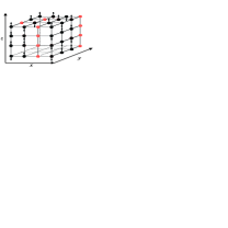
We generate the impurity distribution for a given impurity concentration for a lattice of size in the following way. We compute the integer number of impurity lines of length . We distribute randomly intersections of these lines with the plane, as shown in Fig. 1.
We compute powers of the magnetization ()
| (23) |
where means the lattice summation over all sites. From powers of the magnetization we construct the magnetic susceptibility and Binder cumulant in the following way
| (24) |
| (25) |
Here at first step we perform the thermal averaging of the power of magnetization for each impurity realization (denoted by angle brackets, e.g. ). Then we average these results over different impurity realizations. The averaging over impurity realizations is denoted by the overline. In our simulation we fix , in which case is the inverse temperature.
We compute also the correlation lengths for directions parallel to impurity lines and perpendicular to them with the help of the Fourier transform in a similar way as it was done for isotropic systems.Cooper89 Let us introduce where the wave vector is and we denote , , thermal average of Fourier components for particular realization of impurities. Then we can compute the corresponding correlation lengths averaged over impurity realizations
The simulation is performed with hybrid MC method. LB Each of MC step consists of one flip of Wolff cluster followed by attempts to flip spins in accordance with Metropolis rule.
In our study we deal with a concentration of impurities . Such concentration is very often used in MC simulations of Ising model with disorder,Ballesteros99 ; Prudnikov_MC ; Ivaneyko08 ; Ballesteros98 since in this case concentration of magnetic sites is far from the percolation threshold and from the pure system. Additional empirical reason to take this value of is the following: for 3d Ising model with uncorrelated impurities, correction-to-scaling terms were found to be minimal at concentration of magnetic sites .Ballesteros98
V Results and analysis of simulations
In this section, applying the above described formalism, we give three estimates of the anisotropy exponent obtained from anisotropic FSS predictions for different quantities. From the FSS of susceptibility we get also an estimate for .
V.1 Computation of the correlation length
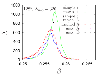
To use relation (21) we need to perform calculations at the critical temperature of an infinite system. Let us assume that the value of the critical temperature of an infinite system is very close to the value of the pseudo-critical temperature of the system with maximal size. In this case that is the temperature of the susceptibility maximum . We perform the computation for a cubical system of size with concentration of impurities . Disorder average may be performed in either of two possible protocols: In the first procedure, at each disorder realization, the temperature dependence of the susceptibility is obtained. Then all these curves are averaged to get a single curve of that depends on . Then the value at which has a maximum is associated with the critical temperature (we refer this way as method A). The second alternative is to average temperatures at which is achieved for each disorder realization (we refer this way as method B).
The results obtained with both methods are given in Fig. 2. The two curves displayed by continuous lines in the figure show behaviour for two separate samples, whereas the dotted curve shows the averaged over 320 samples. Using the method A we first average the susceptibility and then find the point – magenta diamond in Fig. 2. Using the method B we first find a maximum of susceptibility for each disorder configurations, and then average location of these maxima over samples – black square in Fig. 2.
With the value of the critical temperature at hand we can perform a study through relation (21) to extract the anisotropy exponent . To this end, we analyze the correlation length of the system of size varying for both values of . Results of simulations for are given in Fig. 3, where we plot for and directions as function of .
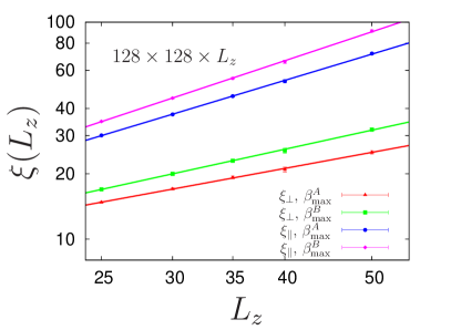
Then we perform the fit of data for in accordance with formulae:
| (27) |
using fitting parameters , . For method A we get , , while for method B we estimate , . Comparing (27) with (21) we get with the following estimates: (method A) and (method B). Taking these values as an accuracy interval of determining, we see that they are in reasonable agreement with existing analytic RG estimates (see Section III).
V.2 Computation of the Binder cumulant
Another way to identify the right value of the exponent is the following. We expect that all curves for the temperature dependence of the Binder cumulant for systems of different sizes but fixed generalized aspect ratio with proper will intersect at the critical point. Therefore we can consider the system of size with and keeping for various values of . For this system we compute the cumulant as a function of the inverse temperature for various values of . At the proper value we expect the intersection of graphs. We perform simulations for , the averaging is performed over realization of impurities.
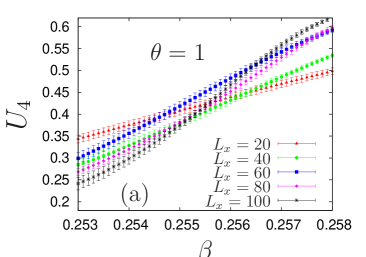
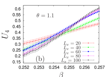
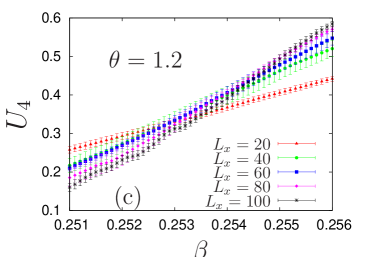
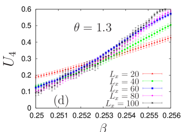
In Fig. 4(a)-(d) we plot the cumulant for values , respectively. Each curve corresponds to averaged over 128 disorder realizations. As one can see, the presence of disorder smears the single crossing point into a region of temperatures where all curves cross. The narrowest region is expected for the value of which is sufficiently close to the real one. To analyze this situation for different values of , we use the following procedure. We split the total set of different impurity realizations onto eight series, and compute the average value (averaged over realizations) of the invariant for each set . Later on we use the averaging over for evaluation of numerical inaccuracy. In Fig. 5(a) we plot for comparison results for as a function of for two different series (lines) and (triangles) for and various sizes . In this figure we observe an important difference between graphs for two series due to impurity induced fluctuations. Our aim is to study the scattering of intersection points. Ideally, graphs for five system sizes should intersect in ten points. In Fig. 5(b) we plot data for and indicate the intersection points by black circles. Here a pair of indexes labels two system sizes for . The graphs for some system sizes have intersections outside of considered interval for , e.g., for and for . In this case we select as “intersection point” the point between left side or right side ends of these two lines selecting the side with the smaller distance between the endpoints.
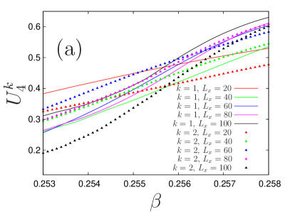
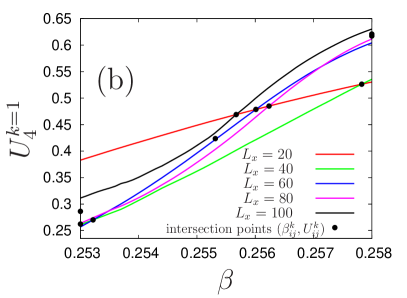
Another possible situation with multiple intersection points may happen due to big scattering of the points in graphs caused by numerical inaccuracy. In this case we perform the averaging over all intersection points and proceed with this averaged point. Then we compute the average values of the inverse temperature
and of the cumulant
over ten intersection points for five system sizes for each set . We observe (as expected), that average of crossing points do not coincide with crossing of average lines.
Now we can compute the average values of the square of deviations from the mean values for the inverse temperature
and for the cumulant
and evaluate numerical inaccuracy. In Fig. 6(a) we plot as a function of .
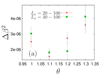
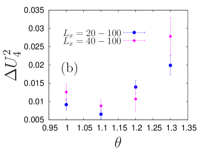
The amplitude of the square of the inverse temperature deviation is about which is consistent with the average distance between points . We do not observe pronounced minima in the interval , and the numerical inaccuracy is comparable with the scattering of the points. In Fig. 6(b) we plot data for the average square of the deviation for the cumulant . The point distribution is very similar to the ones obtained for the inverse temperature. The point for is below its neighbors, but the distance between these points is of the order of the numerical inaccuracy. Therefore the above described procedure corroborates as the optimal one.
V.3 Computations of the susceptibility
In this subsection we describe the results of the computation of the magnetic susceptibility at the critical point with various values of the exponent . Before we obtained two estimates for the critical : (for method A) and (for method B). In Figs. 7(a) and (b) we plot the magnetic susceptibility as a function of the system size in the log-log scale for and , respectively. We expect the power law behavior for the more satisfying value of the exponent . In Fig. 7(a) the deviation of the data from a straight line is less than in Fig. 7(b) therefore we select the estimate for future analysis. This is consistent with the analysis of Binder cumulants where it appears that seems to be out of the crossing window of .
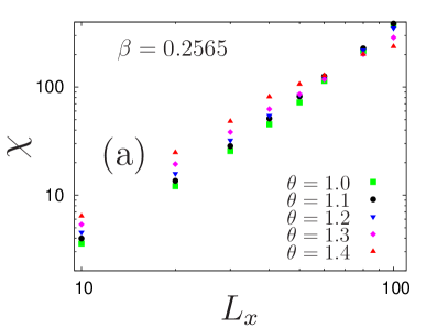
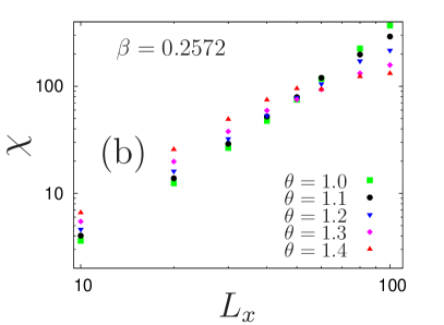
We perform a fit of the magnetic susceptibility by a linear function of in the log-log scale: with and being the parameters of the fit. Then we estimate the deviation of the values of susceptibility measured numerically from those obtained via the fitting function with the help of a chi-square defined as
| (28) |
where is the number of values calculated for values of the system size , is the fitting function, is the appropriate variance defined by the error bars.
The same number of MC steps is used for a given value of the exponent . Therefore, the variance is minimal for small values of the system size and increases for larger values of . The total number of MC steps decreases with increasing of (from for to for ).
The parameter of the fitting procedure characterizes the “quality” of the data with respect to the proposed functional dependence. In our case this parameter describes the deviation of points from the straight line in the log-log representation. We plot as a function of in Fig. 8. The general tendency is the decrease of with an increase of , because due to the smaller number of MC steps the variance is larger in this case.
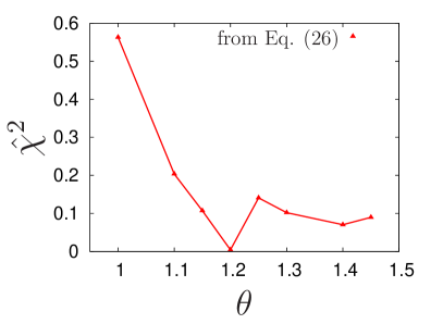
We observe a minimum in the region . Unfortunately, for this procedure we cannot evaluate the variance (inaccuracy) . Therefore we repeat the procedure in more regular way. We split 320 impurity realizations (for each value of for a fixed ) into 10 series and perform the fit by the formula for every series obtaining some value . Then we average these values, compute numerical inaccuracy and plot the results in Fig. 9(a) (black circles for and red triangles for the average value).
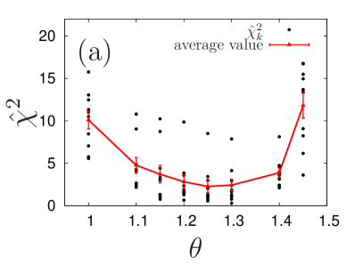
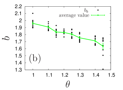
We can see, that reaches the minimum for . In Fig. 9(b) we plot the resulting power as a function of . Value of at gives an estimate for , using the window . We present here also estimate obtained from data of Fig. 9 for the value recognized as an optimal value in subsection V.2 at cumulant analysis.
VI Conclusion
In this paper we have studied by MC simulations the scaling behaviour of thermodynamical quantities in the vicinity of critical point for 3d Ising system with randomly distributed parallel linear extended defects, modeled as non-magnetic impurities collected into lines along spatial direction . We considered combined algorithm using Wolff and Metropolis methods. Our results are consistently interpreted using the theory of anisotropic finite size scaling.
We have estimated the value of the anisotropy exponent using three different methods, namely, from dependence of correlation length on the linear size of the system near the critical point, from a temperature dependence of the fourth-order Binder’s cumulant, from finite-size scaling of the susceptibility. The values estimated are in the range and corroborate RG predictions for the model under consideration.
We have also measured the value of from anisotropic finite-size scaling for the susceptibility. The value reported here is a little bit below the corresponding RG estimates , . Value estimated for is in better agreement with theoretical results. We applied procedure described in this subsection to compute magnetization. However it does not give satisfactory results in this case. This is because magnetization is vanishing quantity at the critical point and therefore it is very sensitive to proper determination of critical temperature.
Finally, let us mention that in spite of the substantial computation effort reported in this paper, the numerical values of the critical exponents are not extremely accurate. This is due to the difficulty of the numerical techniques to deal with anisotropic systems (see e.g. Ref. Chatelain99, ), but from the MC simulations presented in this paper, we believe that we can safely conclude in favor of the anisotropic critical point, since anisotropic scaling is overall nicely confirmed.
Acknowledgements.
This work was supported in part by the 7th FP, IRSES projects No 269139 “Dynamics and Cooperative phenomena in complex physical and biological environments” and No 295302 “Statistical Physics in Diverse Realizations”.References
- (1) Order, Disorder and Criticality, edited by Yu. Holovatch (World Scientific, Singapore,2004); Yu. Holovatch, V. Blavats’ka, M. Dudka, C. von Ferber, R. Folk, T. Yavors’kii, Int. J. Mod. Phys. B, 16, 4027 (2002).
- (2) For the recent reviews on criticality of diluted magnets see e.g.: A. Pelissetto, E. Vicari, Phys. Rep. 368, 549 (2002); R. Folk, Yu. Holovatch, and T. Yavors’kii, Physics - Uspekhi 46, 169 (2003), [Uspekhi Fizicheskikh Nauk 173, 175 (2003)].
- (3) P. E. Berche, C.Chatelain, B. Berche, and W. Janke, Eur. Phys. J. B 39, 463 (2004); B. Berche, P. E. Berche, C.Chatelain, and W. Janke, Condens. Matter Phys. 8, 47 (2005).
- (4) D.P. Belanger and A.P. Young, Jour. Magn. Magn. Mater. 100, 272 (1991).
- (5) W. Janke and M. Weigel, Phys. Rev. B 69, 144208 (2004). J.M. Luck, Europhys. Lett. 24, 359, (1993).
- (6) A review of early work on random anisotropy magnets may be found in: R. W. Cochrane, R. Harris, and M.J. Zuckermann, Phys. Reports 48, 1 (1978). More recent experimental, numerical, and theoretical studies are reviewed in Ref. Dudka05, .
- (7) M. Dudka, R. Folk, and Yu. Holovatch, Journ. Mag. Mag. Mat. 294, 305 (2005).
- (8) A.B. Harris, J. Phys. C 7, 1671 (1974).
- (9) A. Weinrib and B.I. Halperin, Phys. Rev. B 27, 413 (1983).
- (10) E.R. Korutcheva and D.I. Uzunov, Phys. Stat. Sol. (b) 126, K19 (1984), E. Korutcheva and F.J. dela Rubia, Phys. Rev. B 58, 5153 (1998).
- (11) V.V. Prudnikov, P.V. Prudnikov, and A.A. Fedorenko, J. Phys. A 32, L399 (1999); V.V. Prudnikov, P.V. Prudnikov, and A.A. Fedorenko, J. Phys. A 32, 8587 (1999); V.V. Prudnikov, P.V. Prudnikov, and A.A. Fedorenko, Phys. Rev. B 62, 8777 (2000).
- (12) V. Blavats’ka, C. von Ferber, and Yu. Holovatch, Phys. Rev. E 64, 041102 (2001); for recent papers see V. Blavatska, C. von Ferber, and Yu. Holovatch, Phys. Rev. E 83, 011803 (2011) and references therein.
- (13) H.G. Ballesteros and G. Parisi, Phys. Rev. B 60, 12912 (1999).
- (14) V.V. Prudnikov, P.V. Prudnikov, S.V. Dorofeev, and V.Yu. Kolesnikov, Condens. Matter Phys. 8, 213 (2005); V. Prudnikov, P. Prudnikov, B. Zheng, S. Dorofeev, and V. Kolesnikov, Progr. Theor. Phys. 117, 973 (2007).
- (15) D. Ivaneyko, B. Berche, Yu. Holovatch, and J. Ilnytskyi, Physica A 387, 4497 (2008).
- (16) S.M. Dorogovtsev, Fiz. Tverd. Tela (Leningrad) 22, 321 (1980) [Sov. Phys. Solid State 22, 188 (1980)]; S.M. Dorogovtsev, Fiz. Tverd. Tela (Leningrad) 22, 3659 (1980) [Sov. Phys. Solid State 22, 2141 (1980)].
- (17) Y. Gefen, B.B. Mandelbrot, and A. Aharony, Phys. Rev. Lett. 45, 855 (1980); Y.K. Wu and B. Hu, Phys. Rev. A 35, 1404 (1987); Yu. Holovatch, Lecture Notes in Physics, 447, 224, Springer-Verlag, Heidelberg, 1996; Yu. Holovatch and N. Shpot., J. Stat. Phys. 66, 867 (1992); Yu. Holovatch and T. Yavors’kii, J. Stat. Phys. 92, 785 (1998).
- (18) D. Boyanovsky and J.L. Cardy, Phys. Rev. B 26, 154 (1982); D. Boyanovsky and J.L. Cardy, Phys. Rev. B 27, 6971 (1983).
- (19) I.D. Lawrie and V.V. Prudnikov, J. Phys. C 17, 1655 (1984).
- (20) V. Blavats’ka, C. von Ferber, and Yu. Holovatch, Acta Phys. Slovaca 52, 317 (2002).
- (21) V. Blavats’ka, C. von Ferber, and Yu. Holovatch, Phys. Rev. B 67, 094404 (2003).
- (22) V. Blavats’ka, M. Dudka, R. Folk, and Yu. Holovatch, Phys. Rev. B 72, 064417 (2005).
- (23) V.V. Prudnikov, J. Phys. C 16, 3685 (1983).
- (24) V. Blavatska, M. Dudka, R. Folk, and Yu. Holovatch, J. Mol. Liq. 127, 60 (2006).
- (25) B. Berche, P.E. Berche, F. Iglói, and G. Palagyi, Journ. Phys. A: Math. Gen. 31, 5193 (1998).
- (26) J.C. Lee and R.L. Gibbs, Phys. Rev. B 45, 2217 (1992).
- (27) T. Vojta, J. Phys. A: Math. Gen. 36, 10921 (2003); R. Sknepnek and T. Vojta, Phys. Rev. B 69, 174410 (2004).
- (28) Y. Yamazaki, A. Holz, M. Ochiai, and Y. Fukuda, Physica A 150, 576 (1988); Y. Yamazaki, A. Holz, M. Ochiai, and Y. Fukuda, Phys. Rev. B 33, 3460 (1986); Y. Yamazaki, A. Holz, M. Ochiai, and Y. Fukuda, Physica A 136, 303 (1986); Y. Yamazaki, M. Ochiai, A. Holz, and Y. Fukuda, Phys. Rev. B 33, 3474 (1986).
- (29) L. De Cesare and M.T. Mercado, Phys. Rev. 59, 855 (1999).
- (30) A.A. Fedorenko, Phys. Rev. B 69, 134301 (2004).
- (31) L. De Cesare, Phys. Rev. B 49, 11742 (1994); L. De Cesare, M.T. Mercado, Phys. Letts. A 186, 179 (1994); L. De Cesare and M.T. Mercado, Phys. Letts. A 264, 214 (1994).
- (32) A.L. Korzhenevskii, K. Herrmanns, and W. Schirmacher, Phys. Rev. B 53, 14834 (1996).
- (33) M.E. Fisher, in Critical Phenomena, edited by M.S. Green (Academic, New York, 1971).
- (34) M.E. Fisher and M.N. Barber, Phys. Rev. Lett. 28, 1516 (1972).
- (35) M.N. Barber, in Phase Transitions and Critical Phenomena edited by C. Domb and J. Lebowitz (Academic, New York, 1983), Vol.8.
- (36) V. Privman, in Finite Size Scaling and Numerical Simulations of statistical SystemsPhase Transitions and Critical Phenomena edited by V. Privman (Singapore, World scientific, 1990).
- (37) V. Privman and M.E. Fisher, Phys. Rev. B 30, 322 (1984).
- (38) K. Binder, Z. Phys. B 43, 119 (1981).
- (39) K. Kaneda, Y. Okabe, and M. Kikuchi, J. Phys. A, 32, 7263 (1999).
- (40) H.W. Diehl and M. Shpot, Phys. Rev. B 62, 12338 (2000).
- (41) J.-S. Wang, Journal of Statistical Physics 82, 1409 (1996); K. Leung and J.-S. Wang, International Journal of Modern Physics C 10, 853 (1999); K. Leung, International Journal of Modern Physics C 3, 367 (1992); K. Leung and J.L. Cardy, Journal of Statistical Physics 44, 567, (1986).
- (42) A. Hucht, J.Phys. A 35, L481 (2002).
- (43) A. Hucht, Phys. Rev. E 80, 061138 (2009); S. Angst, A. Hucht, and D. E. Wolf, Phys. Rev. E 85, 051120 (2012).
- (44) D. Winter, P. Virnau, J. Horbach, and K. Binder, EPL 91, 60002 (2010).
- (45) A. Hucht and S. Angst, EPL 100, 20003 (2012).
- (46) A. Milchev, M. Müller, K. Binder, and D.P. Landau, Phys. Rev. Lett. 90, 136101 (2003).
- (47) K. Binder and J.-S. Wang, J. Stat. Phys. 55, 87 (1989).
- (48) M. Henkel and U. Schollwöck, J. Phys. A 34, 3333 (2001).
- (49) D.P. Landau and K. Binder, A Guide to Monte Carlo Simulations in Statistical Physics (Cambridge University Press, London, 2005), p. 155.
- (50) F. Copper, B. Freedman, and D. Preston, Nucl. Phys. B 210, 210 (1989).
- (51) H.G. Ballesteros, L.A. Fernández, V. Martín-Mayor, A. Muñoz Sudupe, G. Parisi, and J.J. Ruiz-Lorenzo, Phys. Rev. B 58, 2740 (1998).
- (52) C. Chatelain, P.E. Berche, and B. Berche, Eur. Phys. J. B 7, 439 (1999).