Deep Neural Networks Regularization for Structured Output Prediction

1 Implementation

In this work, we implement our framework throughout a deep neural network. The main supervised task is performed using a deep neural network (DNN) with $K$ layers. Secondary reconstruction tasks are carried out by auto-encoders (AE): the input task is achieved using an AE that has $K_{in}$ layers in its encoding part, with an encoded representation of the same dimension as $\tilde{\mathbf{x}}$. Similarly, the output task is achieved using an AE that has $K_{out}$ layers in its decoding part, with an encoded representation of the same dimension as $\tilde{\mathbf{y}}$. At least one layer must be dedicated in the DNN to link $\tilde{\mathbf{x}}$ and $\tilde{\mathbf{y}}$ in the intermediate spaces. Therefore, $K_{in}+K_{out}<K$.

Parameters $\mathbf{w}_{in}$ are the parameters of the whole input AE, $\mathbf{w}_{out}$ are the parameters of the whole output AE and $\mathbf{w}_{sup}$ are the parameters of the main neural network (NN). The encoding layers of the input AE are tied to the first layers of the main NN, and the decoding layers of the output AE are in turn tied to the last layers of the main NN. If $\mathbf{w}_{i}$ are the parameters of layer $i$ of a neural network, then $\mathbf{w}_{1}$ to $\mathbf{w}_{K_{in}}$ parameters of the input AE are shared with $\mathbf{w}_{1}$ to $\mathbf{w}_{K_{in}}$ parameters of the main NN. Moreover, if $\mathbf{w}_{-i}$ are the parameters of last minus $i-1$ layer of a neural network, then parameters $\mathbf{w}_{-K_{out}}$ to $\mathbf{w}_{-1}$ of the output AE are shared with the parameters $\mathbf{w}_{-K_{out}}$ to $\mathbf{w}_{-1}$ of the main NN.

During training, the loss function of the input AE is used as $\mathcal{J}_{in}$, the loss function of the output AE is used as $\mathcal{J}_{out}$, and the loss function of the main NN is used as $\mathcal{J}_{s}$.

Optimizing Eq.LABEL:eq:eq5 can be performed using Stochastic Gradient Descent. In the case of task combination, one way to perform the optimization is to alternate between the tasks when needed [9, 50]. In the case where the training set does not contain unlabeled data, the optimization of Eq.LABEL:eq:eq5 can be done in parallel over all the tasks. When using unlabeled data, the gradient for the whole cost can not be computed at once. Therefore, we need to split the gradient for each sub-cost according to the nature of the samples at each mini-batch. For the sake of clarity, we illustrate our optimization scheme in Algorithm 1 using on-line training (i.e. training one sample at a time). Mini-batch training can be performed in the same way.

Algorithm 1 Our training strategy for one epoch

1:$\mathcal{D}$ is the shuffled training set. $B$ a sample.

2:for $B$ in $\mathcal{D}$ do

3:     if $B$ contains $\mathbf{x}$ then

4:         Update $\mathbf{w}_{in}$: Make a gradient step toward $\lambda_{in}\times\mathcal{J}_{in}$ using $B$ (Eq.LABEL:eq:eq2).

5:     end if

6:     if $B$ contains $\mathbf{y}$ then

7:         Update $\mathbf{w}_{out}$: Make a gradient step toward $\lambda_{out}\times\mathcal{J}_{out}$ using $B$ (Eq.LABEL:eq:eq3).

8:     end if

9:     # parallel parameters update

10:     if $B$ contains $\mathbf{x}$ and $\mathbf{y}$ then

11:         Update $\mathbf{w}$: Make a gradient step toward $\mathcal{J}$ using $B$ (Eq.LABEL:eq:eq5).

12:     end if

13:     Update $\lambda_{sup}$, $\lambda_{in}$ and $\lambda_{out}$.

14:end for

2 Experiments

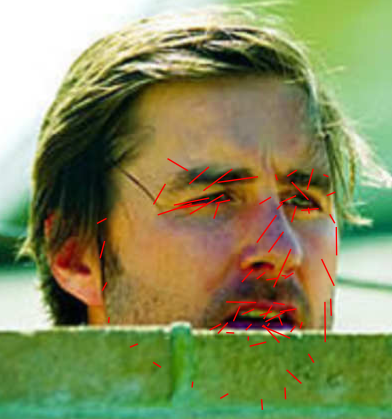
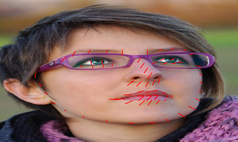
We evaluate our framework on a facial landmark detection problem which is typically a structured output problem since the facial landmarks are spatially inter-dependent. Facial landmarks are a set of key points on human face images as shown in Fig. LABEL:fig:fig0. Each key point is defined by the coordinates $(x,y)$ in the image ($x,y\in\mathbb{R}$). The number of landmarks is dataset or application dependent.

It must be emphasized here that the purpose of our experiments in this paper was not to outperform the state of the art in facial landmark detection but to show that learning the output dependencies helps improving the performance of DNN on that task. Thus, we will compare a model with/without input and output training. [48] use a cascade of neural networks. In their work, they provide the performance of their first global network. Therefore, we will use it as a reference to compare our performance (both networks has close architectures) except they use larger training dataset.

We first describe the datasets followed by a description of the evaluation metrics used in facial landmark problems. Then, we present the general setup of our experiments followed by two types of experiments: without and with unlabeled data. An opensource implementation of our MTL deep instantiation is available online.

2.1 Datasets

We have carried out our evaluation over two challenging public datasets for facial landmark detection problem: LFPW [4] and HELEN [22].

LFPW dataset consists of 1132 training images and 300 test images taken under unconstrained conditions (in the wild) with large variations in the pose, expression, illumination and with partial occlusions (Fig.LABEL:fig:fig0). This makes the facial point detection a challenging task on this dataset. From the initial dataset described in LFPW [4], we use only the 811 training images and the 224 test images provided by the ibug website. Ground truth annotations of 68 facial points are provided by [36]. We divide the available training samples into two sets: validation set (135 samples) and training set (676 samples).

HELEN dataset is similar to LFPW dataset, where the images have been taken under unconstrained conditions with high resolution and collected from Flikr using text queries. It contains 2000 images for training, and 330 images for test. Images and face bounding boxes are provided by the same site as for LFPW. The ground truth annotations are provided by [36]. Examples of dataset are shown in Fig.1.

Figure 1: Samples from HELEN [22] dataset.

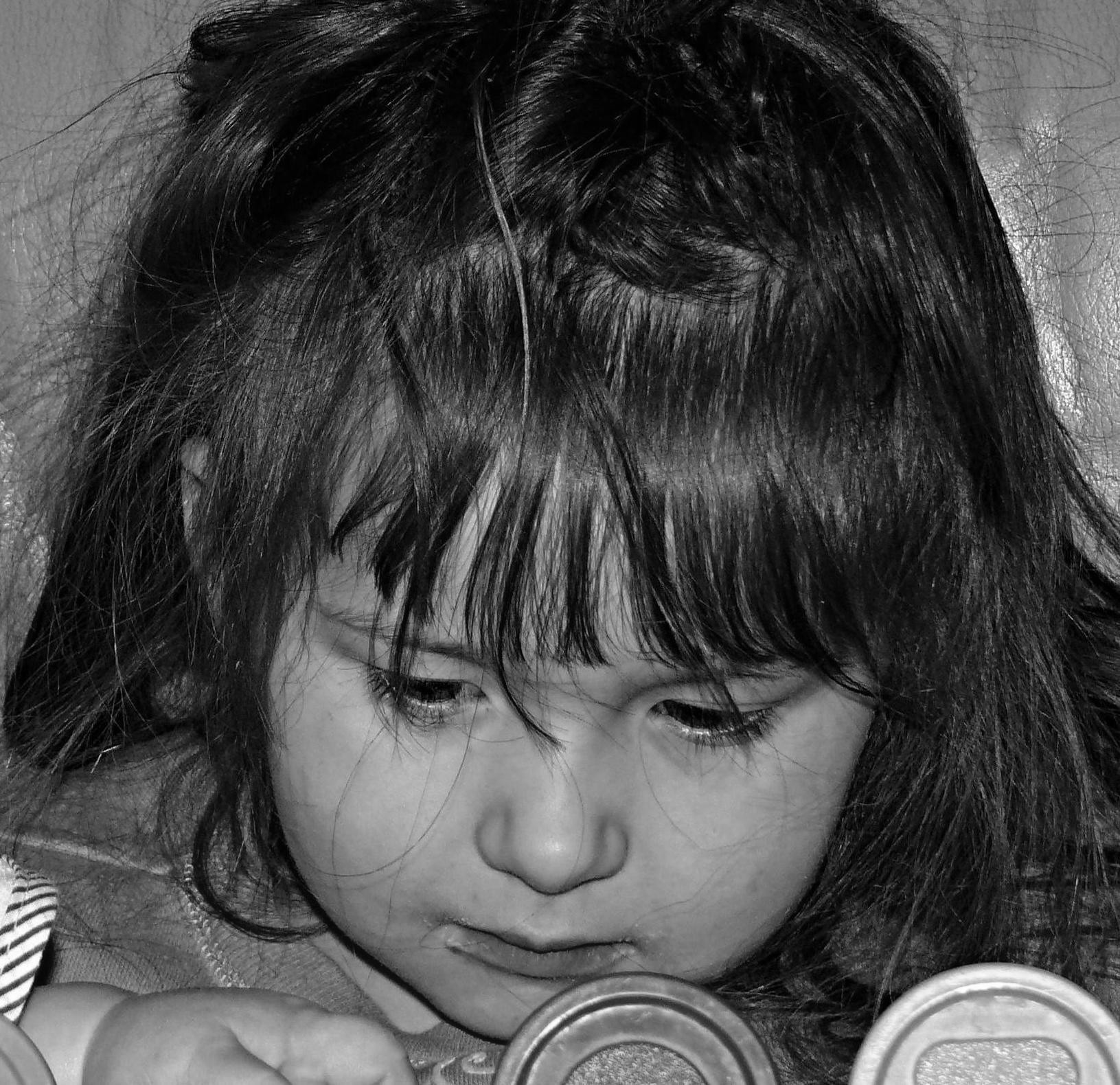
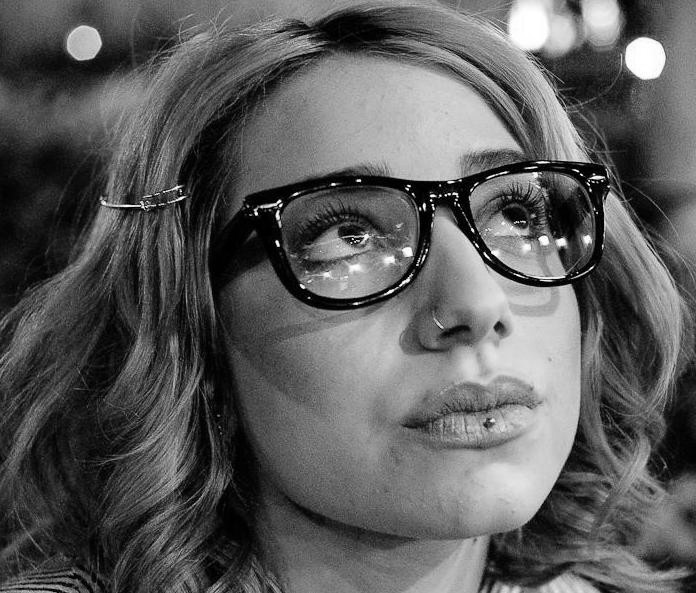
All faces are cropped into the same size ($50\times 50$) and pixels are normalized in [0,1]. The facial landmarks are normalized into [-1,1].

2.2 Metrics

In order to evaluate the prediction of the model, we use the standard metrics used in facial landmark detection problems.

The Normalized Root Mean Squared Error (NRMSE)[10] (Eq.1) is the Euclidean distance between the predicted shape and the ground truth normalized by the product of the number of points in the shape and the inter-ocular distance $D$ (distance between the eyes pupils of the ground truth),

$$NRMSE(s_{p},s_{g})=\frac{1}{N*D}\sum^{N}_{i=1}||s_{pi}-s_{gi}||_{2}\enspace,$$ (1)

where $s_{p}$ and $s_{g}$ are the predicted and the ground truth shapes, respectively. Both shapes have the same number of points $N$. $D$ is the inter-ocular distance of the shape $s_{g}$.

Using the NMRSE, we can calculate the Cumulative Distribution Function for a specific NRMSE ($CDF_{NRMSE}$) value (Eq.2) overall the database,

$$CDF_{x}=\frac{CARD(NRMSE\leq x)}{n}\enspace,$$ (2)

where $CARD(.)$ is the cardinal of a set. $n$ is the total number of images.

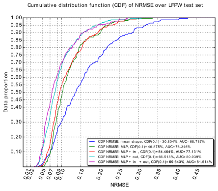
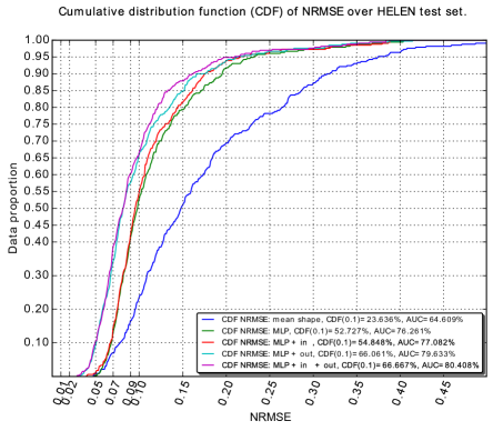
The $CDF_{NRMSE}$ represents the percentage of images with error less or equal than the specified NRMSE value. For example a $CDF_{0.1}=0.4$ over a test set means that $40\%$ of the test set images have an error less or equal than $0.1$. A CDF curve can be plotted according to these $CDF_{NRMSE}$ values by varying the value of $NRMSE$.

These are the usual evaluation criteria used in facial landmark detection problem. To have more numerical precision in the comparison in our experiments, we calculate the Area Under the CDF Curve (AUC), using only the NRMSE range [0,0.5] with a step of $10^{-3}$.

2.3 General training setup

To implement our framework, we use: - a DNN with four layers $K=4$ for the main task; - an input AE with one encoding layer $K_{in}=1$ and one decoding layer; - an output AE with one encoding layer and one decoding layer $K_{out}=1$. Referring to Fig.LABEL:fig:fig0.1, the size of the input representation $\mathbf{x}$ and estimation $\hat{\mathbf{x}}$ is $2500=50\times 50$; the size of the output representation $\mathbf{y}$ and estimation $\hat{\mathbf{y}}$ is $136=68\times 2$, given the 68 landmarks in a 2D plane; the dimension of intermediate spaces $\tilde{\mathbf{x}}$ and $\tilde{\mathbf{y}}$ have been set to 1025 and 64 respectively; finally, the hidden layer in the $m$ link between $\tilde{\mathbf{x}}$ and $\tilde{\mathbf{y}}$ is composed of 512 units. The size of each layer has been set using a validation procedure on the LFPW validation set.

Sigmoid activation functions are used everywhere in the main NN and in the two AEs, except for the last layer of the main NN and the tied last layer of output AE which use a hyperbolic tangent activation function to suite the range $[-1,\;1]$ for the output $\mathbf{y}$.

We use the same architecture through all the experiments for the different training configurations. To distinguish between the multiple configurations we set the following notations:

1. MLP, a DNN for the main task with no concomitant training;

2. MLP + in, a DNN with input AE parallel training;

3. MLP + out, a DNN with output AE parallel training;

4. MLP + in + out, a DNN with both input and output reconstruction secondary tasks.

We recall that the auto-encoders are used only during the training phase. In the test phase, they are dropped. Therefore, the final test networks have the same architecture in all the different configurations.

Beside these configurations, we consider the mean shape (the average of the $\mathbf{y}$ in the training data) as a simple predictive model. For each test image, we predict the same estimated mean shape over the train set.

To clarify the benefit of our approach, all the configurations must start from the same initial weights to make sure that the obtained improvement is due to the training algorithm, not to the random initialization.

For the input reconstruction tasks, we use a denoising auto-encoder with a corruption level of $20\%$ for the first hidden layer. For the output reconstruction task, we use a simple auto-encoder. To avoid overfitting, the auto-encoders are trained using $L_{2}$ regularization with a weight decay of $10^{-2}$.

In all the configurations, the update of the parameters of each task (supervised and unsupervised) is performed using Stochastic Gradient Descent with momentum [41] with a constant momentum coefficient of $0.9$. We use mini-batch size of 10. The training is performed for 1000 epochs with a learning rate of $10^{-3}$.

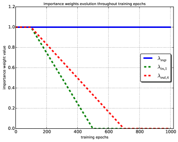
In these experiments, we propose to use a simple linear evolution scheme for the importance weights $\lambda_{sup}$ (supervised task), $\lambda_{in}$ (input task) and $\lambda_{out}$ (output task). We retain the evolution proposed in [3], and presented in Fig.2.

Figure 2: Linear evolution of the importance weights during training.

The hyper-parameters (learning rate, batch size, momentum coefficient, weight decay, the importance weights) have been optimized on the LFPW validation set. We apply the same optimized hyper-parameters for HELEN dataset.

Using these configurations, we perform two types of experiments: with and without unlabeled data. We present in the next sections the obtained results.

2.3.1 Experiments with fully labeled data

In this setup, we use the provided labeled data from each set in a classical way. For LFPW set, we use the 676 available samples for training and 135 samples for validation. For HELEN set, we use 1800 samples for training and 200 samples for validation.

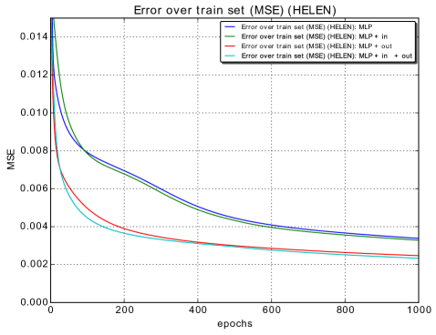
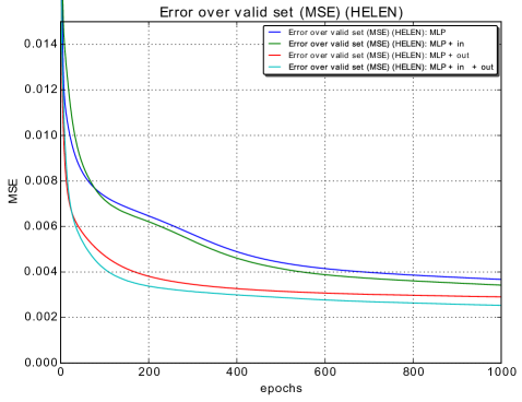
In order to evaluate the different configurations, we first calculate the Mean Squared Error (MSE) of the best models found using the validation during the training. Column 1 (no unlabeled data) of Tab.1, 2 shows the MSE over the train and valid sets of LFPW and HELEN datasets, respectively. Compared to an MLP alone, adding the input training of the first hidden layer slightly reduces the train and validation error in both datasets. Training the output layer also reduces the train and validation error, with a more important factor. Combining the input train of the first hidden layer and output train of the last layer gives the best performance. We plot the tracked MSE over the train and valid sets of HELEN dataset in Fig.5, 5. One can see that the input training reduces slightly the validation MSE. The output training has a major impact over the training speed and the generalization of the model which suggests that output training is useful in the case of structured output problems. Combining the input and the output training improves even more the generalization. Similar behavior was found on LFPW dataset.

At a second time, we evaluate each configuration over the test set of each datasets using the $CDF_{0.1}$ metric. The results are depicted in Tab.3, 4 in the first column for LFPW and HELEN datasets, respectively. Similarly to the results previously found over the train and validation set, one can see that the joint training (supervised, input, output) outperforms all the other configurations in terms of $CDF_{0.1}$ and AUC. The CDF curves in Fig.6 also confirms this result. Compared to the global DNN in [48] over LFPW test set, our joint trained MLP performs better ([48]: $CDF_{0.1}=65\%$, ours: $CDF_{0.1}=69.64\%$), despite the fact that their model was trained using larger supervised dataset (combination of multiple supervised datasets beside LFPW).

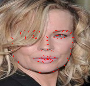
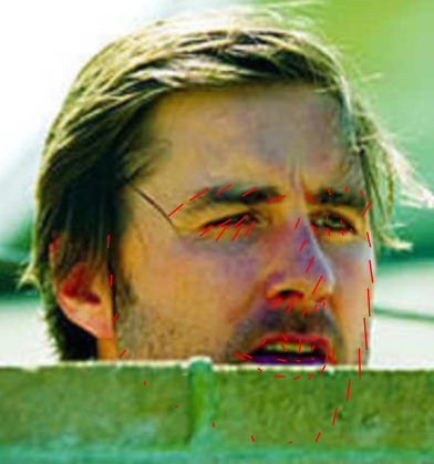
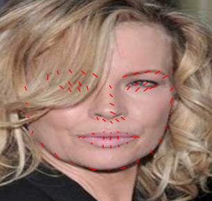
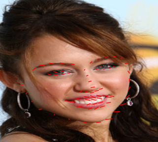
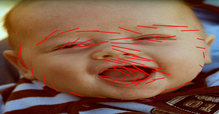
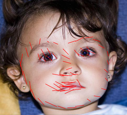
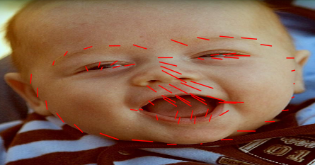
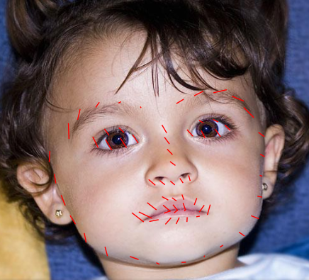
An illustrative result of our method is presented in Fig.3, 4 for LFPW and HELEN using an MLP and MLP with input and output training.

Figure 3: Examples of prediction on LFPW test set. For visualizing errors, red segments have been drawn between ground truth and predicted landmark. Top row: MLP. Bottom row: MLP+in+out. (no unlabeled data)

Figure 4: Examples of prediction on HELEN test set. Top row: MLP. Bottom row: MLP+in+out. (no unlabeled data)

Table 1: MSE over LFPW: train and valid sets, at the end of training with and without unlabeled data.

	No unlabeled data		With unlabeled data
	MSE train	MSE valid	MSE train	MSE valid
Mean shape	$7.74\text{\times}{10}^{-3}$	$8.07\text{\times}{10}^{-3}$	$7.78\text{\times}{10}^{-3}$	$8.14\text{\times}{10}^{-3}$
MLP	$3.96\text{\times}{10}^{-3}$	$4.28\text{\times}{10}^{-3}$	-	-
MLP + in	$3.64\text{\times}{10}^{-3}$	$3.80\text{\times}{10}^{-3}$	$1.44\text{\times}{10}^{-3}$	$2.62\text{\times}{10}^{-3}$
MLP + out	$2.31\text{\times}{10}^{-3}$	$2.99\text{\times}{10}^{-3}$	$1.51\text{\times}{10}^{-3}$	$2.79\text{\times}{10}^{-3}$
MLP + in + out	$2.12\text{\times}{10}^{-3}$	$2.56\text{\times}{10}^{-3}$	$1.10\text{\times}{10}^{-3}$	$2.23\text{\times}{10}^{-3}$

Table 2: MSE over HELEN: train and valid sets, at the end of training with and without data augmentation.

	Fully labeled data only		Adding unlabeled or label-only data
	MSE train	MSE valid	MSE train	MSE valid
Mean shape	$7.59\text{\times}{10}^{-3}$	$6.95\text{\times}{10}^{-3}$	$7.60\text{\times}{10}^{-3}$	$0.95\text{\times}{10}^{-3}$
MLP	$3.39\text{\times}{10}^{-3}$	$3.67\text{\times}{10}^{-3}$	-	-
MLP + in	$3.28\text{\times}{10}^{-3}$	$3.42\text{\times}{10}^{-3}$	$2.31\text{\times}{10}^{-3}$	$2.81\text{\times}{10}^{-3}$
MLP + out	$2.48\text{\times}{10}^{-3}$	$2.90\text{\times}{10}^{-3}$	$2.00\text{\times}{10}^{-3}$	$2.74\text{\times}{10}^{-3}$
MLP + in + out	$2.34\text{\times}{10}^{-3}$	$2.53\text{\times}{10}^{-3}$	$1.92\text{\times}{10}^{-3}$	$2.40\text{\times}{10}^{-3}$

Figure 5: MSE during training epochs over HELEN train (a) and valid (b) sets using different training setups for the MLP.

Figure 6: CDF curves of different configurations on: (a) LFPW, (b) HELEN.

Table 3: AUC and $\mathbf{CDF_{0.1}}$ performance over LFPW test dataset with and without unlabeled data.

	Fully labeled data only		Adding unlabeled or label-only data
	AUC	$\mathbf{CDF_{0.1}}$	AUC	$\mathbf{CDF_{0.1}}$
Mean shape	68.78%	30.80%	77.81%	22.33%
MLP	76.34%	46.87%	-	-
MLP + in	77.13%	54.46%	80.78%	67.85%
MLP + out	80.93%	66.51%	81.77%	67.85%
MLP + in + out	81.51%	69.64%	82.48%	71.87%

Table 4: AUC and $\mathbf{CDF_{0.1}}$ performance over HELEN test dataset with and without unlabeled data.

	Fully labeled data only		Adding unlabeled or label-only data
	AUC	$\mathbf{CDF_{0.1}}$	AUC	$\mathbf{CDF_{0.1}}$
Mean shape	64.60%	23.63%	64.76%	23.23%
MLP	76.26%	52.72%	-	-
MLP + in	77.08%	54.84%	79.25%	63.33%
MLP + out	79.63%	66.60%	80.48%	65.15%
MLP + in + out	80.40%	66.66%	81.27%	71.51%

2.3.2 Data augmentation using unlabeled data or label-only data

In this section, we experiment our approach when adding unlabeled data (input and output). Unlabeled data (i.e. image faces without the landmarks annotation) are abundant and can be found easily for example from other datasets or from the Internet which makes it practical and realistic. In our case, we use image faces from another dataset.

In the other hand, label-only data (i.e. the landmarks annotation without image faces) are more difficult to obtain because we usually have the annotation based on the image faces. One way to obtain accurate and realistic facial landmarks without image faces is to use a 3D face model as a generator. We use an easier way to obtain facial landmarks annotation by taking them from another dataset.

In this experiment, in order to add unlabeled data for LFPW dataset, we take all the image faces of HELEN dataset (train, valid and test) and vice versa for HELEN dataset by taking all LFPW image faces as unlabeled data. The same experiment is performed for the label-only data using the facial landmarks annotation. We summarize the size of each train set in Tab.5..

Table 5: Size of augmented LFPW and HELEN train sets.

Train set / size of	Supervised data	Unsupervised input $\mathbf{x}$	Unsupervised output $\mathbf{y}$
LFPW	676	2330	2330
HELEN	1800	1035	1035

We use the same validation sets as in Sec.2.3.1 in order to have a fair comparison. The MSE are presented in the second column of Tab.1, 2 over LFPW and HELEN datasets. One can see that adding unlabeled data decreases the MSE over the train and validation sets. Similarly, we found that the input training along with the output training gives the best results. Identically, these results are translated in terms of $CDF_{0.1}$ and AUC over the test sets (Tab.3, 4). All these results suggest that adding unlabeled input and output data can improve the generalization of our framework and the training speed.

Acknowledgments

This work has been partly supported by the grant ANR-11-JS02-010 LeMon, the grant ANR-16-CE23-0006 “Deep in France” and has benefited from computational means from CRIANN, the contributions of which are greatly appreciated.

References

- [1] Michael Auli, Michel Galley, Chris Quirk, and Geoffrey Zweig. Joint language and translation modeling with recurrent neural networks. In Proceedings of the 2013 Conference on Empirical Methods in Natural Language Processing, EMNLP 2013, 18-21 October 2013, Grand Hyatt Seattle, Seattle, Washington, USA, A meeting of SIGDAT, a Special Interest Group of the ACL, pages 1044–1054, 2013.
- [2] David Belanger and Andrew McCallum. Structured prediction energy networks. In Proceedings of the 33nd International Conference on Machine Learning, ICML 2016, New York City, NY, USA, June 19-24, 2016, pages 983–992, 2016.
- [3] S. Belharbi, R.Hérault, C. Chatelain, and S. Adam. Deep multi-task learning with evolving weights. In European Symposium on Artificial Neural Networks (ESANN), 2016.
- [4] Peter N. Belhumeur, David W. Jacobs, David J. Kriegman, and Neeraj Kumar. Localizing parts of faces using a consensus of exemplars. In CVPR, pages 545–552. IEEE, 2011.
- [5] Yoshua Bengio, Pascal Lamblin, Dan Popovici, and Hugo Larochelle. Greedy Layer-Wise Training of Deep Networks. In B. Schölkopf, J.C. Platt, and T. Hoffman, editors, NIPS, pages 153–160. 2007.
- [6] Daniel M Bikel, Richard Schwartz, and Ralph M Weischedel. An algorithm that learns what’s in a name. Machine learning, 34(1-3):211–231, 1999.
- [7] R. Caruana. Multitask learning. Machine Learning, 28(1):41–75, 1997.
- [8] Dan C. Ciresan, Alessandro Giusti, Luca Maria Gambardella, and Jürgen Schmidhuber. Deep neural networks segment neuronal membranes in electron microscopy images. In Advances in Neural Information Processing Systems 25: 26th Annual Conference on Neural Information Processing Systems 2012. Proceedings of a meeting held December 3-6, 2012, Lake Tahoe, Nevada, United States., pages 2852–2860, 2012.
- [9] R. Collobert and J. Weston. A unified architecture for natural language processing: deep neural networks with multitask learning. In ICML, pages 160–167, 2008.
- [10] D. Cristinacce and T. Cootes. Feature Detection and Tracking with Constrained Local Models. In BMVC, pages 95.1–95.10, 2006.
- [11] M. El-Yacoubi, M. Gilloux, and J-M Bertille. A statistical approach for phrase location and recognition within a text line: An application to street name recognition. IEEE PAMI, 24(2):172–188, 2002.
- [12] Clément Farabet, Camille Couprie, Laurent Najman, and Yann LeCun. Learning Hierarchical Features for Scene Labeling. IEEE PAMI, 35(8):1915–1929, 2013.
- [13] Moshe Fridman. Hidden markov model regression. PhD thesis, Graduate School of Arts and Sciences, University of Pennsylvania, 1993.
- [14] Alex Graves and Navdeep Jaitly. Towards end-to-end speech recognition with recurrent neural networks. In Proceedings of the 31th International Conference on Machine Learning, ICML 2014, Beijing, China, 21-26 June 2014, pages 1764–1772, 2014.
- [15] Alex Graves, Marcus Liwicki, Santiago Fernández, Roman Bertolami, Horst Bunke, and Jürgen Schmidhuber. A novel connectionist system for unconstrained handwriting recognition. IEEE transactions on pattern analysis and machine intelligence, 31(5):855–868, 2009.
- [16] Judy Hoffman, Dequan Wang, Fisher Yu, and Trevor Darrell. Fcns in the wild: Pixel-level adversarial and constraint-based adaptation. CoRR, abs/1612.02649, 2016.
- [17] Max Jaderberg, Karen Simonyan, Andrea Vedaldi, and Andrew Zisserman. Deep structured output learning for unconstrained text recognition. CoRR, abs/1412.5903, 2014.
- [18] David T. Jones. Protein secondary structure prediction based on position-specific scoring matrices. Journal of Molecular Biology, 292(2):195–202, 1999.
- [19] Andrej Karpathy and Fei-Fei Li. Deep visual-semantic alignments for generating image descriptions. In IEEE Conference on Computer Vision and Pattern Recognition, CVPR 2015, Boston, MA, USA, June 7-12, 2015, pages 3128–3137, 2015.
- [20] Alex Krizhevsky, Ilya Sutskever, and Geoffrey E. Hinton. ImageNet Classification with Deep Convolutional Neural Networks. In F. Pereira, C.J.C. Burges, L. Bottou, and K.Q. Weinberger, editors, Advances in Neural Information Processing Systems 25, pages 1097–1105. Curran Associates, Inc., 2012.
- [21] John D. Lafferty, Andrew McCallum, and Fernando C. N. Pereira. Conditional Random Fields: Probabilistic Models for Segmenting and Labeling Sequence Data. In ICML, pages 282–289, 2001.
- [22] Vuong Le, Jonathan Brandt, Zhe Lin, Lubomir D. Bourdev, and Thomas S. Huang. Interactive Facial Feature Localization. In ECCV, 2012, Proceedings, Part III, pages 679–692, 2012.
- [23] J. Lerouge, R. Herault, C. Chatelain, F. Jardin, and R. Modzelewski. IODA: An Input Output Deep Architecture for image labeling. Pattern Recognition, 2015.
- [24] Xirong Li, Tiberio Uricchio, Lamberto Ballan, Marco Bertini, Cees G. M. Snoek, and Alberto Del Bimbo. Socializing the semantic gap: A comparative survey on image tag assignment, refinement, and retrieval. ACM Comput. Surv., 49(1):14:1–14:39, 2016.
- [25] Shujie Liu, Nan Yang, Mu Li, and Ming Zhou. A recursive recurrent neural network for statistical machine translation. In Proceedings of the 52nd Annual Meeting of the Association for Computational Linguistics (Volume 1: Long Papers), pages 1491–1500, Baltimore, Maryland, June 2014. Association for Computational Linguistics.
- [26] Jonathan Long, Evan Shelhamer, and Trevor Darrell. Fully convolutional networks for semantic segmentation. In IEEE Conference on Computer Vision and Pattern Recognition, CVPR 2015, Boston, MA, USA, June 7-12, 2015, pages 3431–3440, 2015.
- [27] Alireza Makhzani, Jonathon Shlens, Navdeep Jaitly, and Ian J. Goodfellow. Adversarial autoencoders. CoRR, abs/1511.05644, 2015.
- [28] Volodymyr Mnih, Hugo Larochelle, and Geoffrey E. Hinton. Conditional restricted boltzmann machines for structured output prediction. In UAI 2011, Proceedings of the Twenty-Seventh Conference on Uncertainty in Artificial Intelligence, Barcelona, Spain, July 14-17, 2011, pages 514–522, 2011.
- [29] Stéphane Nicolas, Thierry Paquet, and Laurent Heutte. A Markovian Approach for Handwritten Document Segmentation. In ICPR (3), pages 292–295, 2006.
- [30] F. Ning, D. Delhomme, Yann LeCun, F. Piano, Léon Bottou, and Paolo Emilio Barbano. Toward automatic phenotyping of developing embryos from videos. IEEE Trans. Image Processing, 14(9):1360–1371, 2005.
- [31] Hyeonwoo Noh, Seunghoon Hong, and Bohyung Han. Learning deconvolution network for semantic segmentation. In 2015 IEEE International Conference on Computer Vision, ICCV 2015, Santiago, Chile, December 7-13, 2015, pages 1520–1528, 2015.
- [32] Keith Noto and Mark Craven. Learning Hidden Markov Models for Regression using Path Aggregation. CoRR, abs/1206.3275, 2012.
- [33] Franz Josef Och. Minimum error rate training in statistical machine translation. In Proceedings of the ACL, volume 1, 2003.
- [34] Lawrence Rabiner. A tutorial on hidden Markov models and selected applications in speech recognition. Proceedings of the IEEE, 77(2):257–286, 1989.
- [35] Olaf Ronneberger, Philipp Fischer, and Thomas Brox. U-net: Convolutional networks for biomedical image segmentation. In Medical Image Computing and Computer-Assisted Intervention - MICCAI 2015 - 18th International Conference Munich, Germany, October 5 - 9, 2015, Proceedings, Part III, pages 234–241, 2015.
- [36] C. Sagonas, G. Tzimiropoulos, S. Zafeiriou, and M. Pantic. A semi-automatic methodology for facial landmark annotation. In CVPR Workshops, pages 896–903, 2013.
- [37] H. Schmid. Part-of-speech tagging with neural networks. conference on Computational linguistics, 12:44–49, 1994.
- [38] Daniel Dominic Sleator and David Temperley. Parsing English with a Link Grammar. CoRR, 1995.
- [39] Kihyuk Sohn, Honglak Lee, and Xinchen Yan. Learning structured output representation using deep conditional generative models. In NIPS 2015, pages 3483–3491, 2015.
- [40] Bruno Stuner, Clément Chatelain, and Thierry Paquet. Cohort of LSTM and lexicon verification for handwriting recognition with gigantic lexicon. CoRR, abs/1612.07528, 2016.
- [41] I. Sutskever, J. Martens, G. Dahl, and G. Hinton. On the importance of initialization and momentum in deep learning. In ICML, volume 28, pages 1139–1147, 2013.
- [42] Ilya Sutskever, Oriol Vinyals, and Quoc V. Le. Sequence to sequence learning with neural networks. In Advances in Neural Information Processing Systems 27: Annual Conference on Neural Information Processing Systems 2014, December 8-13 2014, Montreal, Quebec, Canada, pages 3104–3112, 2014.
- [43] U. Syed and G. Yona. Enzyme function prediction with interpretable models. Computational Systems Biology. Humana press, pages 373–420, 2009.
- [44] M. Szummer and Y. Qi. Contextual Recognition of Hand-drawn Diagrams with Conditional Random Fields. In IWFHR, pages 32–37, 2004.
- [45] G. Tsechpenakis, Jianhua Wang, B. Mayer, and D. Metaxas. Coupling CRFs and Deformable Models for 3D Medical Image Segmentation. In ICCV, pages 1–8, 2007.
- [46] P. Vincent, H. Larochelle, I. Lajoie, Y. Bengio, and P. Manzagol. Stacked Denoising Autoencoders: Learning Useful Representations in a Deep Network with a Local Denoising Criterion. JMLR, 11:3371–3408, 2010.
- [47] H. Zen, K. Tokuda, and A. Black. Statistical parametric speech synthesis. Speech Communication, 51(11):1039–1064, 2009.
- [48] J. Zhang, S. Shan, M. Kan, and X. Chen. Coarse-to-Fine Auto-Encoder Networks (CFAN) for Real-Time Face Alignment. In ECCV, Part II, pages 1–16, 2014.
- [49] Yang Zhang, Philip David, and Boqing Gong. Curriculum domain adaptation for semantic segmentation of urban scenes. CoRR, abs/1707.09465, 2017.
- [50] Z. Zhang, P. Luo, C. C. Loy, and X. Tang. Facial landmark detection by deep multi-task learning. In ECCV, pages 94–108, 2014.