SUPA, School of Physics and Astronomy, University of Edinburgh, Edinburgh EH9 3FD, United Kingdom
Active Brownian Particles and Run-and-Tumble Particles: a Comparative Study
Abstract
Active Brownian particles (ABPs) and Run-and-Tumble particles (RTPs) both self-propel at fixed speed along a body-axis that reorients either through slow angular diffusion (ABPs) or sudden complete randomisation (RTPs). We compare the physics of these two model systems both at microscopic and macroscopic scales. Using exact results for their steady-state distribution in the presence of external potentials, we show that they both admit the same effective equilibrium regime perturbatively that breaks down for stronger external potentials, in a model-dependent way. In the presence of collisional repulsions such particles slow down at high density: their propulsive effort is unchanged, but their average speed along becomes . A fruitful avenue is then to construct a mean-field description in which particles are ghost-like and have no collisions, but swim at a variable speed that is an explicit function or functional of the density . We give numerical evidence that the recently shown equivalence of the fluctuating hydrodynamics of ABPs and RTPs in this case, which we detail here, extends to microscopic models of ABPs and RTPs interacting with repulsive forces.
1 Introduction
Outside the realm of exact results, and despite recent progress Derrida2007 , non-equilibrium statistical mechanics largely remains (paraphrasing Harish-Chandra Kac ) messy, elusive and non-rigorous. However, we may say (paraphrasing Dyson Kac ) that this is precisely why it is such an interesting research field. While a fully general extension of the well-established framework of equilibrium statistical physics remains out of reach, there are important classes of non-equilibrium systems for which progress towards a comprehensive theory seems achievable. Colloidal self-propelled particles (SPPs), which represent a central focus of research into active matter sriram ; RoP ; romanczuk ; RMP , arguably offer such a prospect. This applies at least in some simplified limits, such as spherical SPPs interacting by central forces only (a restriction that excludes hydrodynamic interactions). In developing theories of such systems, an important general question is how far macroscopic behaviour is sensitive to the detailed dynamical rules. For thermal systems, steady-state properties are governed by Boltzmann equilibrium, and hence sensitive to the energy landscape but not the dynamics used to explore it – so long as this dynamics obeys the principle of detailed balance (as it must do in such cases). For non-equilibrium systems, such as SPPs, the question must be asked afresh. In this article we address this issue, by studying two classes of active particles, ABPs and RTPs. These have related but distinct dynamics, and have become two major workhorses of recent simulation and theoretical studies of active matter. We will find instances where their dynamical differences disappear on coarse-graining, to give the same macroscopic physics; and other instances where these differences remain important – typically when there is short-scale structure in the problem, such as confinement in small traps.
In active matter, a continuous supply of energy destroys microscopic time-reversal symmetry (TRS) and allows phenomena to arise that are impossible in thermal equilibrium systems, where detailed balance restores TRS in the steady state. Inspired in large part by experiments on synthetic self-propelled colloidal particles PennState ; Jones ; golestanian ; Palacci2010PRL ; Bocquet2012 ; bechinger ; palacci ; herminghaus , many recent theory and simulation papers have addressed the physics of a simplified model comprising spherical active Brownian particles (ABPs) fily ; baskaran ; sten1 ; gompper ; sten2 ; speck ; redner ; mallory ; Cristina ; Brady ; Henkes . In parallel, growing experimental interest in bacterial motion Galajda2007 ; Leonardo2010PNAS ; Sokolov2010PNAS ; Saragosti2011PNAS ; Hwa1 ; Vladescu2015PRL ; SchwarzLinek2012PNAS has brought run-and-tumble particles (RTPs) to the fore as a second prototypical model of self-propelled particles at the colloidal scale.
In these models, each particle feels a constant external force oriented along its swim direction . At low density this is equal and opposite to the local drag force felt by a particle moving at speed . (At high density the external force may be partly opposed instead by conservative interparticle forces.) This is a one-body drag and thus the models entirely omit hydrodynamic interactions and all the other physics associated with the presence of an incompressible solvent. These can have important effects, for instance generating self-pumping states Nash2010 ; Stark1 or causing rotation by collision Fielding ; Stark . On the contrary, in the spherical ABP model the angular dynamics comprises rotational diffusion with a fixed diffusivity . Idealized RTPs differ from ABPs only in their rotational relaxation; instead of continuous diffusion, RTPs undergo discrete tumbling events of short duration that completely randomize their swimming direction; these events occur randomly in time at mean rate and the mean time between two tumbles is therefore exponentially distributed 111Other type of distributions, possibly with large tails, may also be considered. See, e.g., Cluzel2004Nature ; ThielPRE2012 . Both models share an important simplification, which would be inadmissible for any particles capable of exerting significant torques on one another (such as non-spherical SPPs at high density). Specifically, the angular dynamics of each particle remains unperturbed by interactions of any kind, and proceeds independent of the positions or orientations of all other particles in the system. In what follows, the terms ABP and RTP refer to this spherical, torque-free case unless stated otherwise.
Another key feature of these two models is that each particle exchanges momentum with external driving and drag forces, not with a suspending solvent. The resulting non-conservation of momentum within the system greatly complicates the discussion of the macroscopic force balances that normally underly mechanical properties such as pressure mallory ; Cristina ; Brady . Indeed, the force per unit area on a wall in general depends on the wall-particle interactions Solon1 ; this dependence does cancel out for the case of spherical (torque-free) ABPs moving with constant propulsive force Solon2 , but not if the propulsive force is itself density-dependent Solon1 (a case we return to below).
In this paper, we present a comparative study of these simplified models of self-propelled particles. We first consider the steady-state distribution of non-interacting SPPs submitted to an external potential . Using exact results on the sedimentation of active particles, we show that ABPs and RTPs each admit an “effective temperature” regime when the Stokes speed is small compared to the swim speed . We show how the effective temperature concept breaks down outside this regime in model-specific ways; this issue has attracted lots of interest recently Palacci2010PRL ; Stark1 ; TailleurCates2009EPL ; Szamel2014PRE ; Ginot2011PRX . We then consider the confinement of SPPs in circular or spherical traps, and show how the different angular dynamics between the two systems result in qualitatively different behaviours outside the effective equilibrium regime.
We then turn to interacting SPPs and consider models that replace interparticle collisions with a density-dependent propulsion force. Therefore we avoid any detailed discussion of the mechanical pressure, although it may offer an interesting alternative perspective on phase equilibria Brady ; Solon2 ; Brady2 . We explore an approximation scheme for torque-free SPPs with collisional interactions whereby the conservative forces responsible for collisional slow-down of the particles are replaced at mean-field level by a “programmed” slow-down, that is, an effective reduction in the propulsive force at high density. This path was first sketched out in TC and pursued further in sten1 ; sten2 ; CT ; Thompson2011JSM ; ModelB . In a more general context it is both legitimate and interesting to consider, in its own right, the case with no conservative force field between particles, and ask about the effects of programmed slow-down among such “ghost” particles. While not forgetting its original motivation in the collisional case, we will often adopt this viewpoint here. Indeed, the concept of a programmed slow-down is well established in biological systems such as bacteria, where density-dependent dynamics can be effectively introduced through a biochemical pathway called quorum sensing RoP ; Hwa1 ; Hwa2 ; quorum . This causes bacteria to change behaviour in response to the concentration of a short-lived chemical that they also emit. Because of the short lifetime, the response is then directly sensitive to the number of neighbours within a short but finite distance, and hence to a local coarse-grained density. Note that this is distinct from chemotaxis Berg ; Schnitzer in which organisms swim preferentially up or down gradients of a long-lived chemical signal—effectively creating a long-range repulsion or attraction. (Chemotaxis might also arise in synthetic, self-phoretic colloids SriramGolestanian .) An interesting study of chemotactic interactions in ABPs, showing some features resembling phase separation of the type discussed below, can be found in Meyer .
In bacteria such as E. coli angular relaxation is an RTP process, for which the consequences of density-dependent speed were first worked out in TC . However, some bacterial types, including mutant strains of E. coli known as “smooth swimmers”, do not tumble. In practice the genetic engineering strategies used in Hwa1 ; Hwa2 to give density-dependent slow-down primarily achieve this by altering tumble times and frequencies (reducing the time-averaged speed). However, were it possible to directly link the actual propulsion speed of bacteria to their local density in a smooth-swimming strain, then this would offer an unambiguous physical realization of ABPs (as opposed to RTPs) with a density dependent speed. As in Hwa1 ; Hwa2 , this could probably be made to happen at densities too low for collisional or crowding effects to be important.
In summary, the study of SPPs with density-dependent propulsion speed is motivated (i) as an approximate representation of the collisional slow-down in SPPs with pairwise repulsions; (ii) as a representation of smooth-swimming or run-and-tumble bacteria with slow-down caused by quorum sensing or a related, non-collisional mechanism; and (iii) as a model in its own right, with which to explore generic collective phenomena in active matter systems. In the last context, it offers further insights into the degree to which macroscopic outcomes depend on local dynamical rules, and we shall focus on this below in comparing the ABP and RTP cases in some detail.
The most striking many-body phenomenon seen in this class of models is motility-induced phase separation, or MIPS. This is by now a well-established concept RoP ; TC ; CT ; Thompson2011JSM ; ModelB ; Farrell2012PRL ; MIPS ; PNAS ; Loewen1 ; Loewen2a and is the result of two effects in combination. First, the mean speed of a motile particle along its propulsion direction decreases with density (in contrast to the equilibrium case where the velocity statistics of a particle are separable, and fixed solely by equipartition). Second, particles tend to accumulate in spatial regions where they move slowly (a possibility ruled out, in isothermal equilibrium, by the fact that the speed distribution cannot depend on position). This combination creates a positive feedback which is the origin of MIPS RoP ; TC ; MIPS .
In what follows, after exploring in Section 2 the one-body behaviour of ABPs and RTPs in external potentials, we turn in Section 3 to their many-body physics, showing first how the large-scale dynamics with density-dependent can in each case be mapped on the equilibrium dynamics of passive particles with attractive forces, and then outlining how gradient terms affect this mapping. Sections 2 and 3 offer a more complete presentation of results reported in TailleurCates2009EPL ; CT respectively. In fact we add substantially to these results: our discussion of ABPs in traps and of angular distributions for ABPs and RTPs under gravity are both new to the current paper. In the many-body section we carefully compare our approach with recent work by others on the role of leading order nonlocality (gradient corrections) in an effective free energy picture. We show further that, somewhat surprisingly, the large-scale equivalence between ABPs and RTPs established at the level of fluctuating hydrodynamics for particles with density-dependent swim speed CT effectively extends to microscopic simulations of ABPs and RTPs interacting with repulsive forces.
2 Steady-state of active particles in external potential
Consider the classical experimental geometry, devised by Jean Perrin, in which dilute colloidal particles are allowed to sediment under gravity in a cuvette. Equilibrium statistical mechanics asserts that we can forget all details of the diffusive dynamics of the colloids: the steady-state probability of finding a particle at a given height is a Boltzmann distribution, , where is the mass difference between the particle and a corresponding volume of liquid 222Note that in all this article but the sedimentation sections, we silently assume the mass of particles to be equal to one.. Let us now replace the Brownian random-walk diffusion of the colloids by an active random walk, powered by some microscopic non-equilibrium process. In the SPP context the latter is a persistent random walk of fixed speed, with either continuous (ABP) or discrete (RTP) changes of direction. (Its persistence length is much longer than for true Brownian motion, although the latter is finite in principle. More importantly, the instantaneous speed of true Brownian motion is not fixed, but has unbounded fluctuations given by the Maxwell-Boltzmann distribution.) Though not identical, clearly the equilibrium and non-equilibrium diffusive processes cannot be completely unrelated, at least in a limit where the persistence length is much smaller than the sedimentation length. Outside this regime, however, very different physics may be encountered.
Previous studies of sedimenting active particles confirm this line of reasoning. Exact results for RTPs in one, two and three spatial dimensions have shown the density profile to be exponential far away from the containing boundaries TailleurCates2009EPL ; TC . The sedimentation length reduces to , with and the inverse mobility of the particle; this result holds in the limit where the sedimentation speed is much smaller than the swim speed .
This effective equilibrium regime, where the sedimentation profile is given by a Boltzmann weight with a temperature independent of the potential , was observed experimentally for ABPs in Palacci2010PRL ; Ginot2011PRX and derived analytically in Stark1 . Its breakdown for stronger confinement, predicted in TailleurCates2009EPL , was not observed experimentally so far Palacci2010PRL ; Ginot2011PRX , triggering a debate about the generic sedimentation behaviour for SPPs Szamel2014PRE . Below, for both RTPs and ABPs (Sections 2.1,2.2) we derive in 2D the full probability distribution for finding a particle at height swimming in direction . The outcome is that ABPs and RTPs both admit the same effective equilibrium regime – up to a simple parameter mapping between and . However, beyond this regime the density profiles are dynamics-dependent, and various definitions of the “effective temperature”, which all coincide within the regime of small , are found to differ beyond it.
In Section 2.4 we turn from sedimentation (which has uniform in space) to address the steady-state distributions of ABPs and RTPs in harmonic traps, where . Again, ABPs and RTPs yield the same limiting effective equilibrium regime but lead to very different physics once the persistence length (respectively or ) is much larger than the trap radius . In this regime, the cases of continuous (ABP) and discrete (RTP) angular rotation give entirely different statistics for the density at the centre of the trap, for reasons we discuss.
2.1 Sedimentation of 2D RTPs
Let us consider the dynamics of a 2D RTP in the presence of an external potential . The self-propulsion velocity is supplemented by a sedimentation velocity so that the master equation reads
| (1) |
We consider a system which is not free-falling, i.e. such that a wall at prevents the particles from crossing this plane. A number of boundary conditions can be used to model the relevant interaction; for example, one can simply cancel the component of the particles velocity Wan2008PRL , or take into account the torque that a wall would exert on actual bacteria TailleurCates2009EPL . Different boundary layer structures then arise proximal to the wall, depending on the details of the dynamics and the boundary condition, which typically show strong particle accumulation in this region Elgeti1 ; Elgeti2 . Beyond this proximal regime (typically a few run lengths in height) a stationary profile is reached at larger whose form is independent of the boundary condition.
In what follows we consider only this distal part of the profile. Its form can be found by assuming a factorized steady-state ; from Eq. 1, the factors must then satisfy
| (2) |
where is a constant, a priori unknown. Eqs. (2) directly give
| (3) |
The constant can then be fixed by the normalization condition , which yields
| (4) |
Finally, the inverse sedimentation length is given by
| (5) |
so that
| (6) |
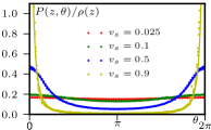
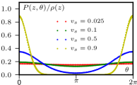
These exact results extend those of TailleurCates2009EPL where only was computed; they perfectly fit simulations of sedimenting RTPs, as shown in figure 1.
2.2 Sedimentation of 2D ABPs
A similar path can be followed for sedimenting ABPs in 2D, starting from the master equation
| (7) |
Again, a separation of spatial and angular variables is confirmed numerically beyond a boundary layer proximal to the wall. The steady-state is found by using the ansatz in Eq.7, to give
| (8) |
which yields
| (9) |
As before, this yields an exponential atmosphere where the inverse sedimentation length is set by the normalisation of . The equation for is the Mathieu equation. Given that is even, it admits the general solution
| (10) |
where is the cosine Mathieu function dlmf . For fixed , this is -periodic in only for a countable subset of values, , which satisfy . Since when , the solution of interest has which implies
| (11) |
Solving this numerically gives . (The numerics can be done using either a formal solver like Mathematica or by procedures based on series expansion of the ’s refsmathieu .) The resulting values of match perfectly the results found by simulating sedimenting ABPs; the full distribution is then obtained by plotting the corresponding Mathieu function, and also agrees very well with the numerics (see Fig 1).
2.3 Effective equilibrium regimes
Boltzmann distributions.
When , both ABPs and RTPs admit an effective equilibrium regime. This is most easily seen for RTPs where can be readily expanded:
| (12) |
Keeping only the dominant contribution, the steady-state thus reduces to the Boltzmann form
| (13) |
where the last equality is an effective Stokes-Einstein relation that connects the mobility to the diffusivity through an effective temperature .
For ABPs, one can use the expansion
| (14) |
to get
| (15) |
Again, the system admits a Boltzmann distribution as steady-state, at the dominant order in , with an effective temperature
| (16) |
Equating the mean time between two tumbles in RTPs and the rotational diffusion time in ABPs, the two effective equilibrium regimes match. (In general dimensions, the parameter mapping is from to , which are the angular autocorrelation times for RTPs and ATPs respectively CT .) However, even the first order corrections in (12) and (15) are different in form (see Fig. 1). Matching the angular relaxation times gives exponential decay of the angular correlator in both cases, but unless the sedimentation length depends on the details of the angular dynamics.
Note that one can also expand the angular distribution close to the effective temperature regime . For 2d RTPs, this gives (using the normalisation )
| (17) | ||||
| (18) |
where on the last line we used that
| (19) |
We can do the same for 2d ABPs using the Fourier expansion of characteristic Mathieu functions dlmf , to get
| (20) | ||||
| (21) |
where on the last line we used that
| (22) |
The difference between for ABPs and RTPs can thus be seen at the level of the second harmonics. As for the difference between the density profiles of RTPs and ABPs, it appears at second order in . Note that the first order correction to however suffices to distinguish these distributions from equilibrium ones.
Fluctuation-dissipation relations.
A quantity that is frequently looked at in non-equilibrium statistical physics is the ratio between correlation and response functions Temperature . Here we examine this for active particles in a sedimentation setup. For simplicity we only consider RTPs where we have explicit formulae, but conceptually what follows applies equally to ABPs. Let us consider a small force applied along and compute the response function
| (23) |
The steady-state distribution is then where is obtained by replacing in Eq. (5). Since , is given by
| (24) |
Since the correlation function , one directly gets
| (25) |
In the effective equilibrium regime, where this gives
| (26) |
which is the usual form for a system with an effective temperature; the system satisfies a fluctuation dissipation theorem (as it should) governed by that temperature.
For larger , the same ratio can be computed explicitly for RTPs using the exact result 5, yielding
| (27) |
In this regime, there is no longer an FDT at temperature for the response to a force along . Moreover, an alternative definition of the effective temperature (which coincides with the fluctuation-dissipation ratio in the effective equilibrium regime) is found by applying a force instead along , and asserting a Stokes-Einstein relation between the mobility and the lateral diffusivity defined via the mean-square displacement along . This yields , just as in Eq.(26), with no dependence at all on . For large , the resulting “horizontal” effective temperature controls neither the density profile nor the fluctuation-dissipation in the direction.
In summary, outside the effective equilibrium regime, the three equally plausible definitions
| (28) |
yield three different effective temperatures. It follows that none is really effective, in the sense that if a new one is needed to describe each property measured, the concept of effective temperature is itself ineffective. In contrast, for both ABPs and RTPs within the effective equilibrium regime (arising in the limit of weak gravity) all three definitions of temperature coincide and the dynamics effectively reduces to an equilibrium problem. For this reason we prefer the term “effective equilibrium” to describe this regime over the less explicit “effective temperature” name used earlier TailleurCates2009EPL .
Interestingly it was recently shown experimentally, by measuring density profiles, that the addition of repulsive interactions between the particles does not immediately destroy the effective equilibrium regime Ginot2011PRX . Note that observing its breakdown experimentally requires a rather large ratio of (for , the difference in is only for ABPs). This may explain why this breakdown has not been reported experimentally so far. The more general question of effective equilibrium in active particles remains a subtle one. For instance, if the fixed self-propulsion speed is replaced by a fluctuating one, using an Ornstein-Uhlenbeck process Szamel2014PRE ; Ginot2011PRX , the effective equilibrium regime extends to arbitrary sedimentation speed , which clearly differs from the RTP and ABP cases treated here. As discussed in TailleurCates2009EPL , fixed propulsion speed is qualitatively different from any dynamics that can sample very high speeds, even if these are rare (as they are in the thermal Maxwell-Boltzmann distribution). One reason for this is clear: if there is a fixed maximum speed, then when exceeds this, all particles are moving only downwards and the sedimentation length must be strictly zero (in the absence of particle-particle interactions). Rare sampling of high molecular speeds is why, in thermal equilibrium, a nonzero sedimentation length is maintained even for very large .
2.4 Trapping of SPPs
Apart from RTPs in one dimension TC , there are no exact results available for the full steady-state distribution of ABPs and RTPs in a harmonic trap. While the approach presented in the previous section does not apply here, because is not factorized, some progress is still possible as we show below. The Stokes velocities of SPPs are now position-dependent and read , where is measured from the center of the trap. The physics is very different from the sedimentation case since the particles are effectively confined to ; At the trapping and propulsive forces compensate exactly, hence preventing the particles from moving further outside.
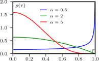
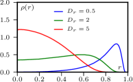
The effective equilibrium regimes correspond to and, as expected, are the same for ABPs and RTPs, with Boltzmann weights for the steady-state distribution (see Fig. 2)
| (29) |
As the ratio between the persistence-length and the trap radius increases, the time needed for the particles to cross the trap becomes much smaller than the mean reorientation time. Particles thus accumulate at the outskirts of the trap where, on average, they point outward radially. How long they persist in this state depends on the dynamical details; in consequence, the density distributions of RTPs and ABPs differ in this regime, particularly in the central region of the trap. Note that, once again, this scenario differs from the fluctuating speed model of Szamel2014PRE where the steady-state in a harmonic trap is always a Gaussian, with fast enough particles reaching arbitrarily large distances and slow enough particles remaining in the center of the trap.
RTP in a harmonic trap.
RTPs pointing outward at the trap boundary undergo instantaneous tumble events at rate whereafter they move across the trap along a certain path. Despite the trap force, and somewhat surprisingly, we show below this path to be a straight line segment, which fully crosses the trap for large ; In this limit, the trajectory is thus a succession of chords of the circle in 2D. The fraction of time spent by a particle in the bulk then corresponds to the fraction of its run-time needed to reach the other side of the trap; this time is proportional to . (This scaling is correct although in practice the path is not followed at constant speed.)
Beyond the scaling in the bulk, one can furthermore compute a limiting shape of as . Let us consider a particle at position on the trap boundary which tumbles to make an angle with the horizontal axis. Its trajectory until the next tumble is simply given by
| (30) |
which generalizes the intuitive result for and . (The latter describes overdamped relaxation across a diameter of the circle to a new equilibrium position opposite the previous one, and applies in the case where the tumble exactly reverses the swim direction.) Eq. (30) describes a linear trajectory joining to , where the trap force balances again the propulsion force. The angular momentum about the initial position satisfies and so that . The velocity and are thus always parallel: the torques about exerted by the trap force and the propulsion force balance to produce a straight trajectory at an angle intermediate between and ; Only the speed is thus varying.
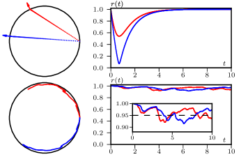
Let us now consider . As shown in Fig. 3, the distance to the center of the trap first decreases from to , which is reached after a time . The distance then increases again until (almost) reaching before the next tumble happens. (Since the speed vanishes as , the particle never reaches exactly the trap boundary.) The trajectory thus crosses twice any annulus of radius within the trap, where it spends a fraction of its duration . Here, we have assumed that the total duration of the trajectory is and are the times at which the particle reaches . These times satisfy
| (31) |
so that the probability of finding a particle at position can be computed as
| (32) |
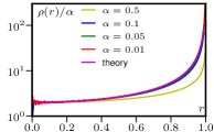
Note that formally diverges as ; in practice this is cut off because the finite duration () of the trajectory ensures that no particle exactly reaches the maximal radius at which its net speed vanishes. The smaller , the closer to the trap boundary this cut-off takes place. We have taken out of the normalization to make the scaling of apparent; is then independent of and equals . The bottom-left quadrant of Fig 2 shows a very good agreement between Eq. (32) and simulations of RTPs for .
ABP in a harmonic trap.
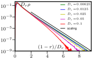
Contrary to RTPs, the orientation of ABPs diffuse slowly so that, as varies, they simply slide along the boundary of the trap, rarely visiting its inner region. This was used recently Yaouen ; Yaouen2 to compute the distribution of ABPs along the boundary of small traps of arbitrary shapes, assuming that the particles effectively never leave the boundary of the trap. As we show below, this asumption is a sound one since the density of particles decreases exponentially as one moves away from the boundary and is exponentially small in at the trap centre. Introducing the angle between the direction of the particle and the normal to the trap , the dynamics in the variables become
| (33) |
where is a Gaussian unit white noise. Using dimensionless variables , , and , Eqs. (33) become
| (34) |
where is also a Gaussian unit white noise. The angle thus undergoes rotational diffusion in an effective potential whose amplitude diverges as . In this limit, oscillates around with Gaussian fluctuations . Consequently, : the particle is almost always at the border of the trap, although the fluctuations of prevent it from reaching exactly (see Fig. 3). The density of particles in the bulk of the trap is thus much smaller than in the RTP case since in a time , the particles are exponentially unlikely to escape the trap boundary while RTPs would typically cross the trap in times . (Recall that these two times are interchangeable in the effective equilibrium regime.) The occurrence of an effective potential, preventing particles from diffusing in angle away from the outward normal direction, at first seems to violate the fact that the dynamics of ABPs is torque-free. Note however that there is no real potential for the angle ; the effective potential for arises not because there is a torque, but because the translational motion of a particle along the trap boundary naturally leads it towards a location where the outward normal is parallel to the current orientation, hence leading to . This effect is also present for RTPs but the discrete angular dynamics effectively allows the RTP to immediately escape the reorientation potential.
To reach the bulk part of the trap, Eq. (34) tells us that needs to climb the effective potential to turn and face its destination. In principle, there are many stochastic paths leading from the boundary to some inner target point at distance from the center. As , however, the transition probability is dominated by the most probable path leading to such a point Tailleur2008JPA (an instanton). The probability of this path will be given by , where is a geometric function depending on the exact location of the target. Since reaching the center of the trap requires a fluctuation of much larger than any required to reach another point close to the trap boundary, the energy barrier increases as the distance of a target from the boundary increases. In practice, a linear function fits very well the effective energy barrier:
| (35) |
where is a dimensionless constant. The density in the center of the trap indeed decreases much faster than for RTPs, as . Somewhat surprisingly, this simple argument gives reasonably good agreement, with a geometric factor whose fit yields , with the bulk density measured in numerical simulations (See Fig. 2).
2.5 Effective equilibrium for generic potentials
In this section we show that for generic potentials , sufficient conditions to observe an effective equilibrium regime are given by
| (36) |
To show this, let us consider a system for which (36) holds. The fluctuating hydrodynamics for ABPs and RTPs in the presence of external drifts derived in CT reads:
| (37) | |||||
| (38) |
where is the surface of the unit sphere in dimensions and equals for RTPs and for ABPs. This description is valid at times and for fields whose gradients are small on the scale of the persistence length of SPPs, ; its derivation in the isotropic case is the subject of section 3, whose notation differs slightly through introduction of a quantity .
Expanding the second term of the r.h.s of Eq. (38) then yields
| (39) |
Equation (39) thus shows that . Using (36), the Laplacian of can then be neglected and (39) simplifies into
| (40) |
The dynamics of is then given by
| (41) |
which is nothing but the equilibrium Fokker-Planck equation of a colloid of mobility subject to an external potential , at a temperature
| (42) |
The steady-state solution of this equation is the Boltzmann weight , which satisfies
| (43) |
which is indeed small, thanks to (36).
The two conditions (36) are enough to show the long time dynamics of the SPP to amount to the equilibrium dynamics of a colloid subject to an external potential . Physically, they require that the Stokes speed be much smaller that the self-propulsion speed of the SPP, but also that its variations over a run-length be much smaller than .
3 Fluctuating Hydrodynamics of ABPs and RTPs
Following CT , we address a model using a general angular relaxation dynamics, combining smooth angular diffusion with diffusivity with pointwise random reorientations (tumbles) at rate . The model has ABPs as one limit and RTPs as another. An intrinsic translational diffusivity is also allowed for; the swim speed is allowed to be position-dependent in the first part of the derivation, , and we will then turn to density-dependent . For a single particle, the probability density of finding the particle at position moving in direction obeys exactly (in )
| (44) | ||||
where is the rotational gradient acting on and the integral is over the unit sphere of area . The first term on the right is the divergence of the advective current resulting from self propulsion and the last two terms are loss and gain due to tumbling out of and into the direction . The second and third terms account for rotational and translational diffusion.
3.1 Coarse-graining procedure
The first part of the derivation below consists in using a moment expansion to show that at large time and space scales, the dynamics (44) amount to a Langevin equation, whose drift and diffusion terms can be fully characterised. Using Itō calculus, we will then start from this single-particle Langevin dynamics to derive a collective Langevin dynamics of the density field of non-interacting active particles. Since all the computations will be done allowing for dependence of the microscopic parameters , , on the spatial position of the active particle, our computation applies to the case where these dependencies occur through the density field . This derivation will thus provide the stochastic dynamics for the density field of interacting active particles. Were we to consider purely ABPs, one could directly use Itō calculus to construct the dynamics of the density field, as was done in Farrell2012PRL ; Romanczuk2012IF ; Peruani2014JSM . In the general case, it is the presence of the tumbles that makes it necessary to take a first diffusive limit. Note that in lattice models, field theoretic methods can be used directly that bypass this limitation and give the same final result Thompson2011JSM .
3.1.1 Moment expansion
We first decompose as
| (45) |
Here, are functions of , which parameterize the zeroth, first and second angular () or spherical () harmonic components of , while projects onto the higher harmonics. Note that in 2 dimensions, the angular harmonics are Fourier sine and cosine series in ; clearly
span the subspaces generated by the first and second harmonics, respectively. The same holds in , where the components of any unit vector are linear combinations of whereas the components of the traceless tensor are linear combinations of .
We now proceed order by order in the harmonics. Integrating Eq. (44) over gives
| (46) |
whereas multiplying eq. (44) by u and then integrating over gives
| (47) |
Finally, multiplying eq. (44) by and integrating over yields
| (48) |
where and , which comes from higher order harmonics, will not play any role in the following. The derivations of Eqs. (46-48) are detailed in Appendix A.
3.1.2 Diffusion-drift equations
So far, beyond the assumed isotropy of and , no approximation has been made; Eqs. (46-48) are exact results for the time evolution of the zeroth, first and second harmonics of . We then note that Eq. (46) is a mass conservation equation:
| (49) |
with a current which involves the first harmonic . We will now use a large time and space scale limit to obtain as a function of .
We first note that is locally conserved and is thus a slow mode: the relaxation of a density perturbation on a scale occurs in a time that diverges as . On the contrary, and are fast modes, whose relaxation rates are given by and . For times greater than , one thus assumes . Eqs. (47) and (48) then give the ordinary differential equations that and satisfy quasi-statically as evolves on time-scales much larger than . By itself, this creates a non-local constitutive relation between and which still involves all harmonics.
Next we explicitly carry out a gradient expansion, yielding for :
| (50) |
from which the quasi-stationary then follows via (47) as
| (51) |
At this order in the gradient expansion, closure is achieved without needing further information on harmonics beyond the first; the current is given by
| (52) |
At this order, Eq.(49) corresponds to a diffusion-drift approximation of the microscopic master equation (44), given by:
| (53) |
where the diffusivity and drift velocity obey
| (54) |
At this level of description, though not for the exact results that preceded it, RTPs and ABPs are seen to be equivalent. That is, in (53), the tumble rate and rotational diffusivity enter only through the combination , so that the two types of angular relaxation are fully interchangeable. Conversely, given a sequence of snapshots showing the large-scale evolution of the local densities of SPPs, one cannot determine whether the system is composed of ABPs or RTPs. Note that “large scale” here excludes some of the trap problems considered in Section 2 where the confinement length is smaller than the persistence length of the self-propelled motion.
3.1.3 Many-body physics
Eqs. (49) and (53) give the evolution for the probability density of one particle at diffusion-drift level. Following TC we can now consider an assembly of particles whose motility parameters and depend on position both directly and indirectly, through a functional dependence on the microscopic density . Since we are considering a multiplicative noise whose variance is a functional of the density field , the construction of the Langevin equation associated to is technically more involved than in the additive case Dean . First, we go from the Fokker-Planck equation (53) to the equivalent Itō-Langevin equation for an individual particle position :
| (55) |
where represents a gradient with respect to the first argument of and not with respect to its implicit dependence on through the field . On the contrary, the operator applies to the functional dependence of on the field and the subscript shows to apply to dependencies on and not on or that may appear in . (For more technical details, see Appendix B.) The two terms form the so-called “spurious drift” term due to the Itō time discretisation. (This term is, of course, not spurious, but necessary once one uses the Itō convention to define that discretization Risken ; oksendal .) The atypical form of this spurious drift is due to depending on both explicitly, which explains the first term, and implicitly—through — which explains the second one. In Appendix B, we show that the density then obeys the many-body Langevin equation TC
| (56) |
with white noise . The gradients in (56) have no subscript ‘’ since there are no more ambiguities at this stage: the derivatives are taken with respect to the spatial coordinate , which does not enter , and not with respect to the position of one of the particles as in (55). Note that when the diffusivity of particle does not include ‘self-interaction’, i.e. or is the result of a convolution between and a symmetric kernel , i.e. , then vanishes (see Appendix B for details) and one recovers the more standard equation
| (57) |
The functionals , and in (54) then define for the interacting particle system the many-body drift velocity and diffusivity and for use in Eq. (56).
Starting from the many-body Itō-Langevin equation (56), one can then derive a functional Fokker-Planck equation for the evolution of the probability density of finding the system with a density field at time :
| (58) |
The technical details, which show the importance of the atypical spurious drift, are detailed in appendix C.
3.1.4 Connection to large-deviation functionals; role of noise
A crucial observation, first made for RTPs in TC , is that (56) reduces, under specific conditions, to a description of passive Brownian particles (PBPs) with a specified free energy functional . (In what follows we use thermal units in which .) This is best seen by noting that the Fokker-Planck equation (58) admits flux-free solution
| (59) |
whenever there exists a functional which satisfies the condition
| (60) |
Indeed, in such a case satisfies (59). As was noted in Peruani2014JSM ; Thompson2011JSM , , with the volume of the system, is the large deviation function of the density profile
| (61) |
It is at first sight very surprising that one can compute this object for any kind of interacting out-of-equilibrium system. However its computability depends on (60) holding true, and indeed this is not true in any general manner. It is however satisfied to leading (zeroth) order in a gradient expansion of . If (60) holds, the system is completely equivalent to an equilibrium system of passive particles with excess chemical potential gradient . This equivalence holds not only at the level of the steady-state but also at the level of the dynamics (58). This means that, at this macroscopic level, the dynamics is effectively an equilibrium one and, for instance, satisfy the Onsager-Machlup symmetry between excursion and relaxation Tailleur2008JPA . However this does not mean that the phenomenology of the system reduces to an equilibrium one. For instance, the slowing down of active particles at high density causes an effective many-body attraction between the equivalent passive particles, characterized by a whose local part has negative curvature in . This kinetic slowdown can trigger a phase separation mechanism, which we detail in the following section, which would be impossible at equilibrium. (Making the viscous drag on each particle an increasing function of local density would generate a similar kinetic slowdown in an equilibrium system, but the Boltzmann distribution would be insensitive to this effect.)
If the condition (60) is not met, however, the dynamics is not equivalent to PBPs with conservative interactions and is therefore “irreducibly” active. As we will show later, the equivalence established above will only hold for homogeneous systems and, when the kinetic slow-down triggers a phase-separation, higher-order gradient terms comes into play at the large-deviation level, and break the mapping to equilibrium.
3.1.5 Mapping to equilibrium
The simplest case is where . Here the left hand side of (60) is and we then require . The simplest first approach is to assume that the functional dependence of swim speed on density is strictly local, so that . We then have where . This structure in the free energy is equivalent to having a passive system whose chemical potential obeys ; the mean particle current then obeys
| (62) |
Noting that in our chosen units () the mobility coincides with the diffusivity , this is the expected form for the stated chemical potential. When is a nonzero constant, the result for generalizes to
| (63) |
This case is explored in MIPS .
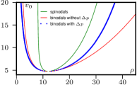
To approximate the excess free energy by a local function is a widely used approximation in equilibrium systems which makes sense at (Landau) mean-field level where fluctuations are neglected. (If the excess free energy were genuinely local, short-length scale fluctuations would be out of control, so to go beyond mean field theory requires treatment of nonlocality even if that is weak). The chosen form (with ) leads to a spinodal instability whenever TC ; MIPS . The system is then equivalent to an equilibrium system undergoing liquid-gas phase separation due to attractive forces and the spinodal instability is complemented by binodals, which can be characterised analytically in some cases (See MIPS for a recent review).
For ABPs with collisions, one finds empirically that with a near-close-packed density beyond which self-propulsion is effectively arrested. The system is then spinodally unstable for fily ; sten1 ; sten2 . Stability is restored by packing constraints at high enough density, but in the present approach (collisions replaced by an effective density-dependent propulsion speed), empirical corrections to are needed to account for this sten1 . An alternative is to impose a sharp cutoff so that for ; this is used in Solon2 .
The presence of a finite , either due to Brownian motion or resulting from the random collision of particles (in which case will depend on ), alters the shape of the spinodal curves which instead obey . This causes the spinodals to meet at a critical point; while in qualitative agreement with the shape of the phase diagram reported for ABPs with repulsions (see, e.g. fily ; sten1 ; redner ), this is somewhat accidental since the actual role of in the simulated dynamics is negligible. The observed critical point is better viewed in terms of the competition between slowing down at high density (promoting motility-induced phase separation) and the buildup of particle mechanical pressure Solon2 . The latter stems primarily from the pair interaction, rather than the small ideal gas part which is proportional to Brady ; Solon2 . Numerically, the spinodals are hard to locate precisely, whereas binodals can be located by looking directly at the coexisting densities in phase-separated states. The point at which phase separate is seen kinetically in ABP simulations often lies in between the spinodal and binodal; it depends in general on nucleation rates and is subject to large finite-size corrections. Very large scale simulations are thus required for accurate phase diagram determination sten1 ; sten2 .
3.1.6 Beyond the local approximation
When a system phase separates, large gradients develop and the gradient expansion cannot be truncated at lowest order: the local approximation to no longer yields a good approximation to the large deviation functional. In such a case, one has to look for higher order gradient terms, which stem from two different mechanisms. First, for real particles, the interactions between particles are never perfectly local: even for hard-core repulsions, the particle size defines a finite interaction range. Second, we have dropped higher angular harmonic contributions by appeal to a gradient approximation. Retaining higher order gradients thus requires two different type of terms whose impact on motility-induced phase separation we now discuss.
Non-local .
The local form of the free energy can be used to predict the binodal densities for phase coexistence via the the common tangent construction on TC . In this construction one equates the chemical potential and the ‘thermodynamic’ pressure in the two phases; this means that a single line can be drawn on a plot of that is tangent at the binodal densities and lies below everywhere else. However, there is a hidden pitfall here: this construction implicitly assumes that, whatever the nonlocal terms are, these continue to obey (60). Whenever they do, a free energy still exists and, so long as it does, the binodal densities do not depend on the precise form of the nonlocal terms. Conversely, if a free energy does not exist, then the binodal conditions can depend explicitly on the nonlocal terms. This is explored in some detail, within the simplification of a effective field theory, in ModelB . For ABPs, numerical evidence of the breakdown of the common tangent construction was reported in sten1 ; sten2 .
The lowest order nonlocal theory can be constructed by assuming that the functional dependence of swim speed on density takes the form TC
| (64) |
This represents a quasi-local dependence on a quantity that samples the local density isotropically in a region of size . For programmed slowing-down (e.g., quorum-sensing) the simplest assumption is that is a density-independent constant. However for collisional slowing down in ABPs, a better estimate is which, with of order unity, is the distance travelled during one angular relaxation time. Substituting the nonlocal form for in (62) gives to leading order
| (65) | |||||
| (66) |
Only if is a constant, independent of density , does this form of chemical potential support the existence of a free energy. If this combination is constant – such as for the case where is constant and TC – then the common tangent can legitimately be used to predict the binodal densities. In all other cases it cannot be relied upon sten1 ; ModelB . Note that in practice, only quantitative differences with the local theory have been noticed when simulating models with such non-local sten1 ; ModelB : the phase separation still occurs, the coarsening law is not much affected, and one only observes quantitative shifts of the binodals. Importantly, the concept of a binodal is maintained: the densities of coexisting phases do not change as the global average density in the system is varied between the two coexistence values.
Other gradient terms.
The second source of higher order gradient terms is the gradient expansion used to close the spherical harmonics expansion in Section 3.1.2. Were we to pursue this gradient expansion to higher orders, we would obtain a set of ordinary differential equations for , , etc. rather than the simple algebraic relation (51) between , and . Solving these equations in terms of and reinjecting into would then not lead to a simple Fokker-Planck equation, from which we would not be able to derive a microscopic Langevin equation like (55), which is the starting point of our approach. The equivalence between ABPs and RTPs at this higher order in gradients is thus questionable. This echoes the fact that the difference between the two models becomes more important at short length scales. As we will show in Section 3.1.7, however, these differences hardly impact the phase diagram.
For ABPs, since one directly starts at the microscopic level with coupled Langevin equations, one can bypass the construction of the microscopic Langevin equation (55) and directly use Itō calculus to obtain a stochastic equation for the probability density of finding particles at going in the direction Farrell2012PRL ; Romanczuk2012IF ; Peruani2014JSM . One then has to project this equation onto successive harmonics and use an appropriate truncation. Again, the equation (56) amounts to second order gradient expansion. It is then easier to pursue this development to higher orders, which would yield coupled stochastic equations for , , , etc.. As far as we are aware, this has not be carried out in the literature for ABPs or RTPs, but progress along this path can be found for aligning nematic particles Bertin2013NJP .
For ABPs, a similar path has been followed at mean-field level, albeit without a proper derivation of the noise terms, to arrive at fily ; Henkes ; Loewen2a
| (67) | ||||
One can then always complete these equation by adding ad-hoc Gaussian noise fily or by assuming that, were the coupled equations (67) to be written in a gradient form (implying the existence of a free energy functional) the noise terms would be whatever is required to give an equilibrium like-dynamics. As we have shown in Section 3.1.4, however, the derivation of the noise terms is a crucial step to determine whether or not the system really maps onto an equilibrium one. Indeed, the integrability criterion (60) is derived by requiring a flux-free steady-state in the Fokker-Planck equation. This condition crucially relies on the fact that the variance of the noise obeys a fluctuation-dissipation relation with the mobility.
Nevertheless, since the derivations of these noise terms are particularly difficult, a first strategy can be to look at whether the equations (67) have the gradient structure of an equilibrium model. While analyzing the linear stability of (67) for a linearly decreasing reveals a spinodal decomposition scenario very similar to the one described in section (3.1.5), it was explicitly shown in Loewen2a that these equations are not of gradient form. However, expanding close to the linear instability, the authors of Loewen2a were able to map these equations onto a Cahn-Hilliard model, but with an effective free energy which depends on where in the phase diagram the expansion is carried out. This revealed a rather surprising feature: the addition of the terms breaks the global mapping to equilibrium but seems to preserve a local one. This however fundamentally changes the structure of the phase diagram: there is nothing to guarantee that the binodals stay in fixed positions as one moves along the ‘tie line’ between them (and without this property the concept of a binodal is inapplicable). Moreover, according to this calculation, a large part of the transition line is changed from a first order to a second order transition, in contrast to the isolated critical point usually seen in liquid-gas type phase-separation.
To test the predictions of this approach, we simulated directly the equations (67) using spectral-methods and semi-implicit time-stepping. We chose a form of which does not lead to at any density and thus does not require an ad-hoc cut-off at the level of the effective free energies:
| (68) |
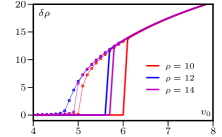
For this choice, we can compute analytically spinodals and binodals predicted by the local theory MIPS and hence evaluate precisely the impact of the term. The scenario revealed by our simulations does not show any of the surprising phenomenology predicted by the methods of Loewen2a : the binodals are quantitatively shifted by this new gradient term, in qualitative agreement with the effect of gradient terms stemming from a non-local ModelB , but the binodals do not vary along the tie-line in the coexistence region (where the lever rule still applies). Also, the transition line seems to remain first-order on approach to the critical point, exhibiting the familiar hysteresis curves (see fig. 4).
In principle, this outcome could depend on our choice of ; note that direct comparison with Loewen2a is not possible since the theory developed there relies on the addition of confining terms at the level of the free energy that do not exist at the level of the PDE, Eq. (67). However this interpretation seems unlikely given the growing breadth of literature supporting the existence of well-defined binodals in MIPS. An alternative possibility is that the new and unusual phenomenology predicted from the approach of Loewen2a is an artefact of a quasi-linear, noiseless treatement of what is in fact a noisy nonlinear transition. Further study is needed to resolve this issue, for instance by carrying out the analytical procedure in Loewen2a for the particular chosen in (68).
3.1.7 Comparison between microscopic simulations of RTPs and ABPs
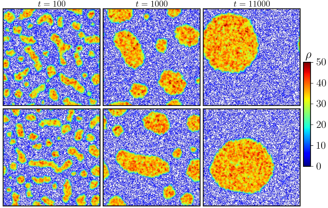
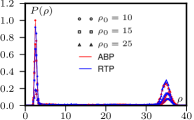
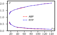
Since gradient terms can alter the equivalence between ABPs and RTPs, we carried out extensive microscopic simulations of MIPS for both models in two dimensions for particles in an square domain. We first compared the two models in the case of a density-dependent swim speed given by (68). The coarsening of both phase separating systems is shown in figure 5 and shows a strikingly similar dynamics. Beyond the apparent similarity of the two dynamics, one can compute the steady-state density distributions of the two systems in the phase separated region, which shows that both the mean densities and their fluctuations in each phase are also very similar (see Fig. 6). Note that as expected, the coexisting densities along the tie-line in the coexistence region do not depend on the mean density .
We then simulated both ABPs and RTPs in the case where slowing down is caused by repulsive interactions (represented as a WCA potential as in fily ; baskaran ; sten1 ). We know that the theory correctly captures the slowdown in these models but that it lacks the direct interparticle forces which are responsible for saturating density in the high-density phase Solon2 . Therefore, the dynamical equivalence of ABPs and RTPs at large scales might break down for the repulsive case where much of the physics depends on short-distance collisional events taking place below the coarse-graining length scale of the fluctuating hydrodynamics theory. Suprisingly however, the phase diagrams of repulsive ABPs and RTPs collapse onto each other upon the usual rescaling (see Fig. 6). Thus, although we have shown that the details of the angular dynamics are important for SPPs confined to traps of size comparable to the run-length or smaller, the presence of short-length scale physics in the mechanism for MIPS does not create a similar dependence on details, as judged either by the qualitative kinetic observations or a quantitative study of phase diagrams.
4 Conclusions
Motivated by a wish to understand for active systems the relation between microscopic dynamics and macroscopic behaviour, we have in this paper compared in detail two distinct but related classes of self-propelled particles: Active Brownian particles and run-and-tumble particles. These differ only in the details of their angular relaxation (continuous versus discrete). We considered first one-body-problems involving non-interacting particles in either uniform fields (e.g., gravity) or isotropic harmonic traps. In both cases, for weak enough forces there is an “effective equilibrium” regime in which the characteristic length scale set by the balance of external and propulsive forces is large compared to the run length, defined as the distance a free particle can travel during its orientational relaxation time. In this regime, the two types of dynamics (ABP and RTP) are equivalent modulo a simple mapping between parameters, which corresponds to equating the angular relaxation time in the two cases. However, for stronger confinement the corrections to this picture are specific to the chosen dynamics. In the case of harmonic traps, this difference is particularly striking: in the regime where the confinement length is large compared to the run length, there is an exponentially strong suppression of the density of ABPs at the trap centre when compared to RTPs of the same rotational relaxation time. This can be attributed to a subtle but physically simple mechanism whereby, in the strong trapping regime, particles tend to remain a long time at the outer edge of the trap, where external and propulsive forces balance. For RTPs this balance is suddenly destroyed with each tumble event, whereas for ABPs, which update their orientations gradually, there is a tendency to drift around the perimeter so that the balance is continually maintained, causing only an exponentially small escape rate from the surface region. We also considered the effect of the microscopic rotational dynamics on MIPs, or motility-induced phase separation. For this process we gave a fuller presentation of results summarized in our earlier papers concerning the derivation of collective equations for the particle density field, from which criteria for MIPS are easily found within a limiting approximation corresponding to neglect of gradient terms in the large deviation functional. This criterion is again insensitive to the choice of rotational dynamics. It is explicitly derived from a model where particles interact through a programmed dependence of their propulsion speed on the local density, but also describes, to reasonable accuracy, the case where slowing down is caused instead by collisions. We then considered the role of gradient corrections, arising either from nonlocality in the dependence of speed on density, or as additional terms in a combined expansion in spatial gradients and angular harmonics of the local distribution of particle orientations. Although the latter could in principle cause qualitative shifts in phase behaviour, in common with previous studies we do not find compelling evidence for anything more than a quantitative shift numerically. Specifically, although the “equilibrium” conditions for phase coexistence (those derivable from the local part of the large deviation functional) are violated, the system still exhibits conventional binodals whose defining property is that the density of coexisting phases is independent of the intermediate global density of the system. For the case where MIPS is caused by collisional rather than programmed speed reduction, we find, somewhat surprisingly, that there is once again almost no difference in phase behaviour between ABPs and RTPs with matched angular relaxation time. This is despite the fact that both the collisional dynamics, and the presence of sharp interfaces in the system, involve length scales below those at which the equivalence of the two models can be formally established by systematic coarse graining.
Acknowledgements: The authors thank Rosalind Allen, Ludovic Berthier, Cecile Cottin-Bizonne, Paul Goldbart, Davide Marenduzzo, Joakim Stenhammar and Raphael Wittkowski for discussions. MEC thanks the Royal Society for a Research Professorship. This work was supported in part by EPSRC Grant EP/J007404/1.
Appendix A Moment-expansion
We start from the master equation on the probability density :
| (69) |
with the rotational part of the Laplacian acting on . We then use the decomposition (45) of , which we recall here for clarity
| (70) |
In the following we will use the notation and the convention that repeated indices are implictly summed upon: . Because enters solely through the combination , it can always be chosen traceless symmetric. (Indeed, replacing by or does not change this sum.)
We will use the standard notation for the scalar product on the sphere
| (71) |
for which spherical (and angular) harmonics are orthogonal. To obtain equations for , , , we take the scalar product of equation (69) with , and . To do so, we compute
| (72) |
which rely on
| (73) | ||||
Projecting (69) on 1 then yields for
| (74) |
while projecting (69) on yields for
| (75) |
The last two terms are easy to compute since . Then, spherical and angular harmonics of order are eigenvectors of with eigenvalues and , respectively, and the projection on selects the term so that
| (76) |
The first term of the r.h.s. of (75) is harder to compute since is not directly developed in harmonics. It can however be brought to a simpler form:
| (77) | ||||
Note that always applies to everything on its right, unless specified otherwise. One then obtain for the evoluation of
| (78) |
Next, one projects (69) on to obtain
| (79) |
for the left hand side, and for the r.h.s.
| (80) |
Again, the last two terms are simple since . Only the second angular/spherical harmonics survive the projection on ; they are eigenvectors of , with eigenvalues for d=3 and for . Hence the rotational diffusion term contributes a factor
| (81) |
Again, the first term of (80) is slightly more difficult to handle and has to be split as
| (82) | ||||
where we have introduced which comes from the projection of on the second harmonics and whose precise expression we won’t need.
Appendix B From microscopic to mesoscopic Itō-Langevin equations
Itō drift with functional dependences.
The total gradient of with respect to , notated as for lack of a better notation, is given by the chain rule
| (84) |
where the first term on the r.h.s. comes from the explicit dependence of on and the second from the dependence of on which itself depends on . By convention, is thus a “partial gradient” which acts upon the explicit dependence of on (its first argument) but not on its implicit dependence through . Using the explicit expression of , one has
| (85) |
Equation (85) shows why the notation , which indicates that the gradient acts on and not on or , is essential—though cumbersome—to get the correct result. Inserting (85) into (84) and integrating by parts, one then finds that
| (86) | ||||
As a consistency check, and to understand how the operator works, let us consider a simple example where the diffusivity of a particle at position is a linear functional of the density of its neighbours, convoluted by some kernel :
| (87) |
In such a case, the total gradient of with respect to can be directly computed:
| (88) |
where is the standard gradient of the function . Applying the formula (86), one finds
| (89) |
where the first term comes from the explicit derivative and the second one from the functional derivative. Note that, in the latter term, does not act upon . The computation can now be readily pursued, to give
| (90) |
Using again that and integrating by parts, one gets
| (91) |
Interestingly, the functional derivative generates a term which will be absent whenever is a symmetric kernel or when the particles are not self-interacting. (By this we mean that the diffusivity of particle is a function of and a functional of ; as such it is functionally dependent only on the density field of other particles, which differs from the total density by the -function self-term.) For complete generality however, we must retain this term in the Langevin equation (55) and throughout the construction of the Langevin equation for , in order to derive a Fokker-Planck equation which is properly ordered as this is crucial to get the correct steady-state. Since the contribution of this term vanishes in many cases, it is often silently omitted in the literature.
Let us further note that, looking at the simple derivation of equation (88), all ambiguities can be overcome by coming back to the microscopic definition of . As often with functionals, the notational problem is present only when working at the field level, where it stems from an underlying ambiguity concerning the gradient symbol , which is used in different contexts to represent either a total derivative (acting on both implicit and explicit dependences of , and hence containing in practice a functional derivative) or a partial derivative acting only on the first argument of . This ambiguity translates into an ordering problem at the level of the Fokker-Planck equation. However, at the large deviation level—which corresponds here to the large size limit—we are effectively interested in the small noise limit of our stochastic partial differential equations. The various ordering of the Fokker-Planck equation differ by terms, similar to those that distinguish Itō and Stratonovich time-discretisation, which are generally negligible Tailleur2008JPA . This is why the issue was for instance (rightly) neglected in Peruani2014JSM .
Mesoscopic Langevin equation.
Let us now consider a function and compute the time evolution of where is solution of the Langevin equation (55). Using Itō’s formula Risken ; oksendal , one finds
| (92) |
where
| (93) |
Introducing and using that, for any function , , Eq. (92) can be rewritten
| (94) |
where the derivatives in and are now taken with respect to . The last term in (94), even though it looks harmless, requires some explanations. Indeed, has dependencies on both through its explicit dependence and through its functional dependence on . When going from (92) to (94), we use that
| (95) |
where we have replaced all the ’s by but the one in , i.e., has not been replaced by . There is thus no dependence of on through . From now on, gradients are not ambiguous anymore: they solely apply to the first argument of which is the only place where depends on . There is thus no need anymore for the notation . Integrating by part Eq. (94) then leads to
| (96) |
Alternatively, can also be written
| (97) |
Since the equations (96) and (97) hold for any function , one gets
| (98) |
Introducing the Gaussian white noise
| (99) |
whose statistics satisfy
| (100) |
one gets
| (101) |
which is Eq. (56) as required.
Appendix C Functional Fokker-Planck Equation
The easiest way to derive the Fokker-Planck equation (58) starting from the Langevin equation (56) is to spatially discretize the latter in one spatial dimension
| (102) |
where
| (103) | ||||
| (104) |
Note that we use centred differences to respect the isotropy of the equation. One can then use the general relation between Itō-Langevin dynamics and the Fokker-Planck equation Risken ,
| (105) |
to derive the Fokker-Planck equation satisfied by . To do so, we first note that
| (106) | ||||
| (107) |
To (slightly) lighten the notation, we write for the operator . The second order differential operator then becomes
Shifting by the indices in the two sums, one finally gets
| (108) |
We now have to compute the drift term in the Fokker-Planck equation . Noting that is a gradient, , where can be read in (103), the drift term can be rewritten
| (109) | ||||
Putting everything together yields
| (110) |
Let us now note that commutes with but not , since the latter is in principle a function of all the ’s. However, the application of on exactly cancels the one before last term in (110), so that
Taking at this stage the continuum limit and integrating once by part yields the correct Fokker-Planck equation
| (111) |
where one has recognised the operator
| (112) |
Equation (112) is actually the best way to make sense of this operator and to see that the gradient really applies to the field with respect to which we are taking a functional derivative and not to the argument of this functional derivative. The equation (111) directly generalizes to (58) in higher dimensions. We note that to get the correct ordering between and in the Fokker-Planck equation, it was necessary to correctly account for the atypical form of the spurious Itō drift as defined in the main text.
References
- (1) B. Derrida, J. Stat. Mech. P07023 (2007).
- (2) M. Kac. Enigmas of Chance: an Autobiography, Univ of California Press (1985).
- (3) S. Ramaswamy, Annu. Rev. Cond. Mat. Phys. 1, 323 (2010).
- (4) Cates M. E., Rep. Prog. Phys. 75,042601 (2012).
- (5) P. Romanczuk, M. Baer, W. Ebeling, B. Lindner, L. Schimansky-Geier, Eur. Phys. J. Special-Topics 202, 1 (2012).
- (6) M. C. Marchetti, J.-F. Joanny, S. Ramaswamy, T. B. Liverpool, J. Prost, M. Rao, R. A. Simha, Rev. Mod. Phys. 85, 1143 (2013).
- (7) W. F. Paxton, S. Sundararajan, T. E. Mallouk, A. Sen, Ang. Chimie - Int. Ed. 45, 5420 (2006).
- (8) J. R. Howse, R. A. L. Jones, A. J. Ryan, T. Gough, R. Vafabakhsh, R. Golestanian, Phys. Rev. Lett. 99, 048102 (2007).
- (9) R. Golestanian, T. B. Liverpool, A. Ajdari, New J. of Phys. 9, 126 (2007).
- (10) J. Palacci, C. Cottin-Bizonne, C. Ybert, L. Bocquet, Phys. Rev. Lett. 105, 088304 (2010).
- (11) I. Theurkauff, C. Cottin-Bizonne, J. Palacci, C. Ybert, L. Bocquet, Phys. Rev. Lett. 108, 268303 (2012).
- (12) I. Buttinoni, J. Bialké, F. Kümmel, H. Löwen, C. Bechinger, T. Speck, Phys. Rev. Lett. 110, 238301 (2013)
- (13) J. Palacci, S. Sacanna, A. P. Stenberg, D. J. Pine, P. M. Chaikin, Science 339, 936 (2013).
- (14) S. Thutupalli, R. Seeman, S. Herminghaus, New J. Phys. 13, 073021 (2011).
- (15) Y. Fily, M. C. Marchetti, Phys. Rev. Lett. 108, 235702 (2012).
- (16) G. S. Redner, M. F. Hagan, A. Baskaran, Phys. Rev. Lett. 110, 055701 (2013).
- (17) J. Stenhammar, A. Tiribocchi, R. J. Allen, D. Marenduzzo, M. E. Cates, Phys. Rev. Lett. 111, 147502 (2013).
- (18) A. Wysocki, R. G. Winkler, G. Gompper, Europhys. Lett. 105, 48004 (2014).
- (19) J. Stenhammar, D. Marenduzzo, R. J. Allen, M. E. Cates, Soft Matter 10, 1489 (2014).
- (20) T. Speck, J. Bialké, A. M. Menzel, H. Löwen, Phys. Rev. Lett. 112, 218304 (2014).
- (21) G. S. Redner, A. Baskaran, M. F. Hagan, Phys. Rev. E 88, 012305 (2013).
- (22) S. A. Mallory, A. Saric, C. Valeriani, A. Cacciuto, Phys. Rev. E 89, 052303 (2014).
- (23) X. B. Yang, L. M. Manning, M. C. Marchetti, Soft Matter 10, 6477 (2014).
- (24) S. C. Takatori, W. Yan, J. F. Brady, Phys. Rev. Lett. 113, 028103 (2014).
- (25) Y. Fily, S. Henkes, M. C. Marchetti, Soft Matter 10, 2132 (2014).
- (26) P. Galajda, J. Keymer, P. Chaikin, R. Austin, J. Bacteriol. 189, 8704 (2007); P. Galajda et al., J. Modern Optics 55, 3413-3422 (2008).
- (27) R. Di Leonardo, L. Angelani, D. Dell’Arciprete, G. Ruocco, V. Iebba, S. Schippa, M. P. Conte, F. Mecarini, F. De Angelis, E. Di Fabrizio, Proc. Natl. Acad. Sci. USA 107, 9541 (2010).
- (28) A. Sokolov, M. M. Apodaca, B. A. Grzybowski, I. S. Aranson, Proc. Natl. Acad. Sci. USA 107, 969 (2010).
- (29) J. Saragosti, V. Calvez, N. Bournaveas, B. Perthame, A. Buguin, P. Silberzan, Proc. Natl. Acad. Sci. USA 108, 16235 (2011).
- (30) C. Liu, X. Fu, L. Liu, X. Ren, C. K. L. Chau, S. Li, L. Xiang, H. Zeng, G. Chen, L.-H. Tang, P. Lenz, X. Cui, W. Huang, T. Hwa, J.-D. Huang,Science 334, 238 (2011).
- (31) I. D. Vladescu, E. J. Marsden, J. Schwarz-Linek, V. A. Martinez, J. Arlt, A. N. Morozov, D. Marenduzzo, M. E. Cates, W. C. K. Poon, Phys. Rev. Lett. 113, 268101 (2014).
- (32) J. Schwarz-Linek, C. Valeriani, A. Cacciuto, M. E. Cates, D. Marenduzzo, A. N. Morozov, W. C. K. Poon, Proc. Natl. Acad. Sci. USA 109, 4052 (2012).
- (33) R. W. Nash, R. Adhikari, J. Tailleur, M. E. Cates, Phys. Rev. Lett. 104, 258101 (2010).
- (34) M. Enculescu, H. Stark, Phys. Rev. Lett. 107 058301 (2011).
- (35) R. Matas-Navarro, R. Golestanian, T. B. Liverpool, S. M. Fielding, Phys. Rev. E. 90, 032304 (2014).
- (36) A. Zoettl, H. Stark, Phys. Rev. Lett. 112, 118101 (2014).
- (37) E. Korobkova, T. Emonet, J. M. G. Vilar, T.S. Shimizu, P. Cluzel, Nature 428, 574 (2004).
- (38) F. Thiel, L. Schimansky-Geier, I. M. Sokolov, Phys. Rev. E 86, 021117 (2012).
- (39) A. P. Solon, Y. Fily, A. Baskaran, M. E. Cates, Y. Kafri, M. Kardar, J. Tailleur, arXiv:1412.3952 (2014).
- (40) A. P. Solon, J. Stenhammar, R. Wittkowski, M. Kardar, Y. Kafri, M. E. Cates, J. Tailleur, Phys. Rev. Lett., In press, arXiv:1412.5475 (2014).
- (41) J. Tailleur, M.E. Cates, EPL 86, 60002 (2009).
- (42) G. Szamel, Phys. Rev. E 90, 012111 (2014).
- (43) F. Ginot, I. Theurkauff, D. Levis, C. Ybert, L. Bocquet, L. Berthier, C. Cotton-Bizonne, Phys. Rev. X 5 011004 (2015).
- (44) S. C. Takatori, J. F. Brady, Phys. Rev. E 91, 032117 (2015).
- (45) J. Tailleur, M. E. Cates, Phys. Rev. Lett.100, 218103 (2008).
- (46) M. E. Cates, J. Tailleur, EPL 101, 20010 (2013).
- (47) A. G. Thompson, J. Tailleur, M. E. Cates, R. A. Blythe, J Stat. Mech. P02029 (2011).
- (48) R. Wittkowski, A. Tiribocchi, J. Stenhammar, R. J. Allen, D. Marenduzzo, M. E. Cates, Nature Commun. 5, 4351 (2014).
- (49) Fu X. et al, Phys. Rev. Lett. 108, 198102 (2012).
- (50) M. B. Miller, B. L. Bassler, Ann. Rev. Microbiol. 55, 165 (2001).
- (51) H. C. Berg, E. coli in Motion Springer, NY (2004).
- (52) M. J. Schnitzer, Phys. Rev. E 48, 2553 (1993).
- (53) S. Saha, R. Golestanian, S. Ramaswamy, Phys. Rev. E 89, 062316 (2014)
- (54) M. Meyer, L. Schimansky-Geier, P. Romanczuk, Phys. Rev. E 89, 022711 (2014).
- (55) F. D. C. Farrell, J. Tailleur, D. Marenduzzo, M. C. Marchetti, Phys. Rev. Lett. 108, 248101 (2012).
- (56) M. E. Cates, J. Tailleur, Ann. Rev. Cond. Matt. Phys. 6, 219 (2015).
- (57) M. E. Cates, D. Marenduzzo, I. Pagonabarraga, J. Tailleur, Proc. Nat. Acad. Sci. USA 107, 11715 (2010).
- (58) J. Bialké, T. Speck, H. Löwen, Phys. Rev. Lett. 108, 168301 (2012).
- (59) T. Speck, J. Bialké, A. M. Menzel, H. Löwen, Phys. Rev. Lett. 112, 218304 (2014).
- (60) M. B. Wan, C. O. Reichhardt, Z. Nussinov, C. Reichhardt, Phys. Rev. Lett. 101, 018102 (2008).
- (61) J. Elgeti, G. Gompper EPL (Europhysics Letters) 85, 38002 (2009).
- (62) J. Elgeti, G. Gompper, EPL (Europhysics Letters) 101, 48003 (2013).
- (63) J. Elgeti, G. Gompper, EPL (Europhysics Letters) 109, 58003 (2015).
- (64) The Digital Library of Mathematical Functions, http://dlmf.nist.gov/28
- (65) F. A. Alhargan, SIAM Review 38, 239-255 (1996).
- (66) L. F. Cugliandolo, J. Phys. A 44, 3001 (2011). D. Loi, S. Mossa, L. F. Cugliandolo, Physical Review E 77 051111 (2008); D. Loi, S. Mossa, L. F. Cugliandolo, Soft Matter 7 3726 (2011).
- (67) Y. Fily, A. Baskaran, M. F. Hagan, Soft Matt. 10, 5609 (2014).
- (68) Y. Fily, A. Baskaran, M. F. Hagan, Phys. Rev. E 91, 012125 (2015).
- (69) J. Tailleur, J. Kurchan, V. Lecomte, J. Phys. A 41, 50500 (2008).
- (70) P. Romanczuk, L. Schimansky-Geier, Interface focus 2, 746 (2012).
- (71) J. Barré, R. Chétrite, M. Muratori, F. Peruani, J. Stat. Phys. 158 589 (2015).
- (72) D. S. Dean, J. Phys. A. Math. Gen. 29, L613 (1996).
- (73) H. Risken, The Fokker-Planck Equation: Methods of Solution and Applications, Springer Verlag, Berlin (1996).
- (74) B. K. Oksendal, Stochastic Differential Equations: An Introduction with Applications, 5th Edn., Springer Verlag, Berlin (2000)
- (75) E. Bertin et al., New J. Physics 15, 085032 (2013).