Cosmological parameters from the comparison of peculiar velocities with predictions from the 2M++ density field
Abstract
Peculiar velocity measurements are the only tool available in the low-redshift Universe for mapping the large-scale distribution of matter and can thus be used to constrain cosmology. Using redshifts from the 2M++ redshift compilation, we reconstruct the density of galaxies within 200 Mpc, allowing for the first time good sampling of important superclusters such as the Shapley Concentration. We compare the predicted peculiar velocities from 2M++ to Tully-Fisher and SNe peculiar velocities. We find a value of 0.431 0.021, suggesting 0.401 0.024, in good agreement with other probes. The predicted peculiar velocity of the Local Group arising from the 2M++ volume alone is km s-1, towards , , only out of alignment with the Cosmic Microwave Background dipole. To account for velocity contributions arising from sources outside the 2M++ volume, we fit simultaneously for and an external bulk flow in our analysis. We find that an external bulk flow is preferred at the 5.1 level, and the best fit has a velocity of towards , . Finally, the predicted bulk flow of a 50 Mpc Gaussian-weighted volume centred on the Local Group is 230 30 km s-1, in the direction , , in agreement with predictions from CDM.
1 Introduction
Peculiar velocities, i.e. deviations in the motions of galaxies from the Hubble flow, are valuable tools which probe the underlying distribution of dark matter, and are in fact the only practical means of doing so on large scales in the low redshift Universe. They can be used to constrain the amplitude of matter density fluctuations on a range of scales. As the amplitude of such fluctuations are themselves cosmology-dependent, the analysis of peculiar velocities provides a direct means of testing cosmological predictions.
In the current standard cosmological paradigm, the observed structure in the Universe is a result of gravitational instabilities which grew from density perturbations in an otherwise homogeneous background. This gravitational attraction of objects to surrounding structure results in peculiar motion, i.e. motion in addition to that resulting from the expansion of the Universe. Assuming only mass continuity and standard gravitation in an expanding universe, in the linear regime where these fluctuations in density are small, i.e. , peculiar velocities are proportional to gravitational accelerations. This relation, as expressed in integral form, is as follows:
| (1) |
where is the peculiar velocity field, is the mass density contrast, is the cosmological density parameter, and where distances are measured in km s-1 (i.e. , where is the Hubble parameter and is the comoving distance in Mpc). The growth rate of density perturbations, , is generally parameterized by , where for CDM (Wang & Steinhardt, 1998), which has recently been shown to be consistent with observations (Hudson & Turnbull, 2012).
As the total matter density contrast cannot be observed, however, to make use of Equation (1), an assumption must first be made as to how observed galaxies trace the underlying total matter. Assuming linear biasing holds on large scales, , where is the linear bias factor, and where we have used the subscript “” when referring to galaxies. Rewriting Equation (1) in terms of the observable density contrast of galaxies in the nearby Universe, the proportionality factor between gravitational acceleration and peculiar velocity is then . Thus, if linear theory holds, by comparing measured peculiar velocities to those predicted by the distribution of galaxies in redshift surveys, one can constrain cosmological parameters through the measurement of . Furthermore, under the assumption of linear biasing , where is the root mean square density fluctuations on an 8 Mpc scale.
By measuring directly from the redshift data, one can eliminate and constrain the degenerate cosmological parameter combination . Using this method of velocity-velocity comparison, a number of recent studies have constrained this parameter combination (Pike & Hudson, 2005; Davis et al., 2011; Branchini et al., 2012; Turnbull et al., 2012).
In addition to constraints placed on these parameters, when full sky surveys are used one can compute the velocity of the Local Group (hereafter LG) arising from the volume under consideration as predicted by linear theory. While it has long been assumed that the dipole in the Cosmic Microwave Background (CMB) temperature map is a Doppler effect due to the Sun’s motion, this has only been proved recently, via the aberration of the CMB temperature anisotropies (Planck Collaboration et al., 2013b). The motion of the Sun with respect to the Galaxy and of the Galaxy with respect to the barycentre of the LG are well known (e.g. Courteau & van den Bergh 1999), and when combined with the Sun’s motion with respect to the CMB (Hinshaw et al., 2009) allows a determination of the motion of the LG with respect to the CMB: in the direction , . A deviation from the predicted value with that derived from the CMB dipole would presumably arise from sources beyond the survey and would thus have implications for large scale structure. As the tidal field falls off as , to first order one can model additional velocity contributions to the LG arising from sources outside the survey volume as a dipole, with the magnitude of this dipole, or residual bulk flow, itself being a test for cosmological models. Past studies constraining cosmological parameters through comparison of predicted motion of the LG using linear theory and that derived from the CMB include Erdoğdu et al. (2006), and Bilicki et al. (2011). Recently such an analysis has been extended to the non-linear regime using a novel orbit-reconstruction algorithm to predict motions of nearby objects (Lavaux et al. 2010).
In addition to reconstructing the motion of the Local Group, one can explore the bulk motion of a large volume (typically the mean velocity of a 50 Mpc Gaussian-weighted window) as such motion probes the amplitude of matter power spectrum on large scales. As previous studies in this vein have found hints of excess power on large scales (cf. Watkins et al. 2009), there has been interest in performing such analyses using peculiar velocity surveys (e.g. Turnbull et al., 2012; Hong et al., 2014).
In this work we explore the methods used to self-consistently reconstruct the real space density field from redshift space while quantifying any biases intrinsic to this reconstruction method. We then use the recently constructed large full-sky 2M++ catalogue composed of 69,160 galaxy redshifts to measure to high precision and constrain . We further explore the growth of the LG’s dipole as predicted by linear theory arising from structures within 2M++, in addition to computing the bulk flow arising from this survey.
This paper is organized as follows: in §2 we briefly review construction of the 2M++ catalogue, we discuss accounting for incompleteness and functional dependence of galaxy bias on luminosity when computing the density field, and we outline details of the reconstruction procedure. In §3 we explore the growth of the LG velocity amplitude arising from 2M++ as a function of survey depth. In §4 we discuss peculiar velocity surveys used, the methods used in comparing predicted velocities to measured velocities, as well as the results obtained from such analyses. We discuss and compare our results to those from recent literature in §5, and conclude in §6.
2 Density Field Reconstruction
Redshift surveys measure positions of objects in redshift-space. As Equation (1) requires real-space positions, we must first map observed redshifts to real-space distances. The observed redshift, , is related to cosmological redshift resulting from the expansion of the Universe, , and that resulting from peculiar velocities, , through
| (2) |
where for non-relativistic peculiar motions . Note that in the above if is corrected to some frame of reference, such as the CMB, then is the peculiar velocity with respect to that frame. The comoving distance in the low-redshift Universe is then related to the cosmological redshift through
| (3) |
(Peebles 1993) where is the comoving distance, is the local value of the Hubble parameter, and where is the local value of the deceleration parameter, which is given by for a flat CDM Universe. As real-space positions are dependent on peculiar velocity predictions, which are themselves dependent on real-space positions, mapping redshifts to real-space must be done with care.
In this section, we discuss the 2M++ redshift catalogue, and outline the procedure used in reconstructing comoving positions of the galaxies therein. §2.1 reviews construction of 2M++, and in §2.2 we outline how galaxy weights were computed to account for the fact that 2M++ is magnitude limited. In §2.3 we briefly review the choice of smoothing kernel. We discuss the procedure used to normalize the smoothed density field to the same effective bias in §2.4. In §2.5 we outline the iterative scheme used to recover real-space positions from redshift-space, and in §2.6 we take a cosmographic tour through the recovered density field.
2.1 2M++ Redshift Compilation
The integral in Equation (1) is over all space. In reconstructing the velocity field of the local Universe, therefore, clearly one would like a redshift survey that is very deep and as close to all-sky as possible. Two such catalogues which have been used extensively in the past include the sparsely sampled IRAS Point Source Catalogue Redshift Survey (PSCz, Saunders et al. 2000), and more recently, the shallower but more densely sampled Two-Micron All-Sky Redshift Survey (2MRS, Huchra et al. 2012). In this work we use a superset of 2MRS, dubbed 2M++, constructed by Lavaux & Hudson (2011). This sample has greater depth than 2MRS, and superior sampling than PSCz. The photometry is from the Two-Micron-All-Sky-Survey (2MASS) Extended Source catalogue, (2MASS-XSC, Skrutskie et al. 2006), an all-sky survey in the , and bands. Redshifts in the band of the 2MASS Redshift Survey (2MRS) are supplemented by those from the Sloan Digital Sky Survey Data Release Seven (SDSS-DR7, Abazajian et al. 2009), and the Six-Degree-Field Galaxy Redshift Survey Data Release Three (6dFGRS, Jones et al. 2009). Data from SDSS was matched to that of 2MASS-XSC using the NYU-VAGC catalogue (Blanton et al., 2005). As 2M++ draws from multiple surveys, galaxy magnitudes from all sources were first recomputed by measuring the apparent magnitude in the band within a circular isophote at 20 mag arcsec-2. Following a prescription described in Lavaux & Hudson (2011), magnitudes were then corrected for Galactic extinction, cosmological surface brightness dimming and stellar evolution. After corrections the sample was limited to in regions not covered by 6dFGRS or SDSS, and limited to elsewhere.
Other relevant corrections which were made to this catalogue include accounting for incompleteness due to fibre-collisions in 6dF and SDSS, as well as treatment of the zone of avoidance (ZoA). Incompleteness due to fibre-collisions was treated by cloning redshifts of nearby galaxies within each survey region as described in Lavaux & Hudson (2011).
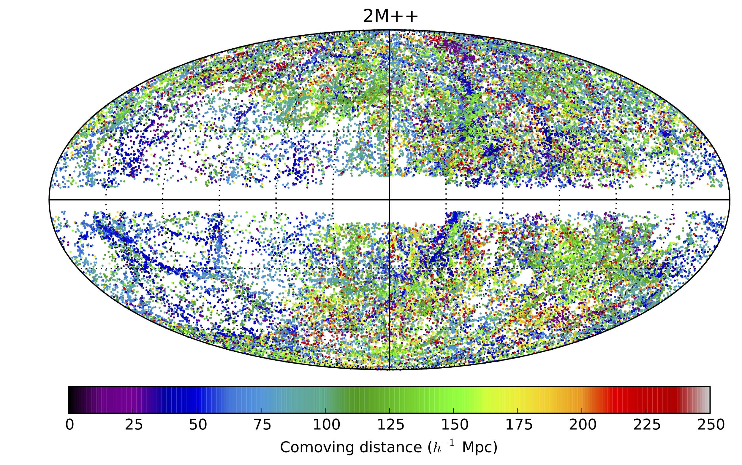
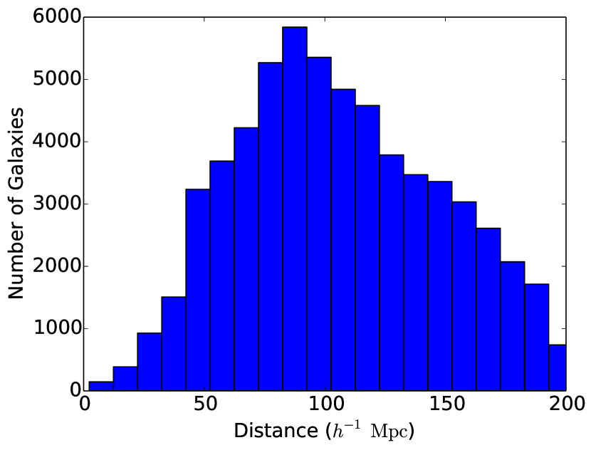
In treating the ZoA, for Galactic longitudes in the range [30∘, 330∘], lower latitudes (5∘) were first masked and then cloned with the redshifts from 2MRS in an equal-area strip just above the missing northern () Galactic strip, and, for the negative Galactic latitudes in the south, a strip below that was cloned. Near the Galactic centre, for longitudes in the range [-30∘, 30∘], the wider Galactic latitude strip 10∘ was filled with the redshifts from 6dFGRS in a similar way. A histogram of distances is shown in Figure 1.
2.2 Luminosity Function & Galaxy Weights
Before using the catalogue to construct the density field, we must first account for survey incompleteness. In this section we provide a summary of the method used to obtain the luminosity function fit to the catalogue; this luminosity function is in turn used to in the weighting scheme employed to account for incompleteness. For a complete description of these calculations as applied to this catalogue see Lavaux & Hudson (2011). The luminosity function used to characterize the dataset is the Schechter function (1976), which when written in terms of absolute magnitudes is given by:
| (4) |
where is the density normalization, is the absolute magnitude break, and is additional power-law parameter to be determined. Schechter function parameters are computed using likelihood formalism, where the product of all conditional probabilities of observing galaxies intrinsic magnitudes is maximized given their redshifts, Schechter parameter values, and survey completeness at their specified angular positions and distances.
Before computing weights we first discuss the different ways by which we can model the galaxy density contrast. As we cannot compute the mass density contrast of observed galaxies directly, we must use either the number-density of galaxies, or their luminosity-density in computing . In the context of linear biasing, our goal is to create a galaxy density contrast field which most closely traces the underlying total mass density contrast. Although luminosity-density may be a better proxy for stellar mass, and thus for the underlying mass distribution of dark matter, we will consider both schemes in this work.
To account for incompleteness, galaxies are weighted according to a common prescription similar to that of Davis & Huchra (1982). In the case of a number-density scheme, observed galaxies are weighted to account for the number of galaxies not observed at a given distance due to the magnitude limit of the survey. When using the galaxy number-density for a single homogeneous redshift survey, galaxies are weighted by
| (5) |
when , and unity otherwise. The flux limit, , corresponds to a band apparent magnitude limit of 11.5 for galaxies drawn from 2MRS and 12.5 otherwise. The luminosity used above corresponds to a band absolute magnitude of . Computed weights used in this work additionally account for the inhomogeneous incompleteness of 2M++ and a complete description of their determination can be found in Lavaux & Hudson (2011).
In this paper, by default, we will use luminosity-density to compute the galaxy density contrast. The weight assigned to each galaxy’s luminosity is again based on the fraction of the total luminosity expected, given the magnitude limit of the survey, to the luminosity one expects to observe at a given distance. Thus, for a single homogeneous redshift survey, galaxy luminosities are weighted by
| (6) |
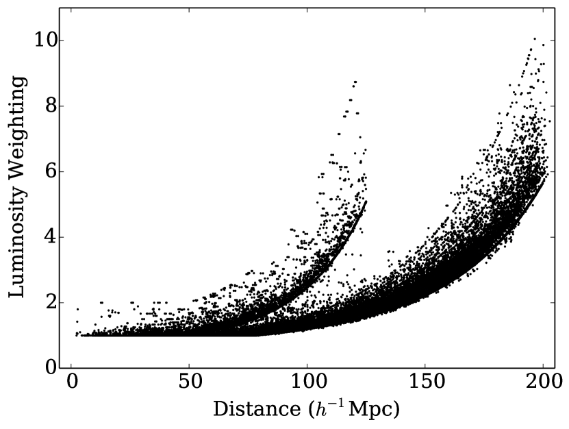
The calculated luminosity weights obtained for the best values of cosmological parameters are shown in Figure 2.
2.3 Smoothing
In order to use Equation (1), the density field must first be sufficiently smooth for linear theory to apply. The optimal scale on which to smooth the data was determined by comparing velocities from an N-body simulation to predictions obtained through linear theory using different smoothing lengths. Smoothing the density contrast with a 4 Mpc Gaussian was found to be the best compromise in minimizing the scatter in predicted velocities vs. simulation velocities, while simultaneously returning an unbiased slope in the comparison of observed nonlinear velocities (from the simulation) with the linear theory predictions from a smoothed, reconstructed density field of halos. These comparisons are discussed in greater detail in Appendix A.
2.4 Accounting for Magnitude Dependence of Galaxy-Matter Bias
For magnitude limited surveys such as 2M++, the mean luminosity of observed galaxies increases with depth. As galaxy-matter bias has been found to increase with luminosity, this means that objects observed at higher redshift are on average more biased than those observed nearby. In this section we account for this effect by rescaling the density field to the same effective bias. We do so using the bias model of Westover (2007) in which bias is a function of luminosity. By comparing the correlation function of 2MASS volume-limited subsamples, converting the binned absolute magnitude to a luminosity and defining , Westover (2007) found , where is the bias of an galaxy. This result is consistent with that of Norberg et al. (2001) and Tegmark et al. (2002), who did similar analyses using projected correlation functions of 2dFGRS and the SDSS power spectrum, respectively.
Since bias is a function of luminosity, this means that a naive computation of the density field using a magnitude limited survey would lead to a larger effective bias at larger distances. As our end goal is to compare predicted velocities with measured velocities and determine , we must first correct the density contrast field by normalizing the field to the same effective bias. The effective number-weighted bias is computed as follows:
| (7) |
Using a luminosity-weighting scheme in computing the density contrast, the effective luminosity-weighted bias is given by:
| (8) |
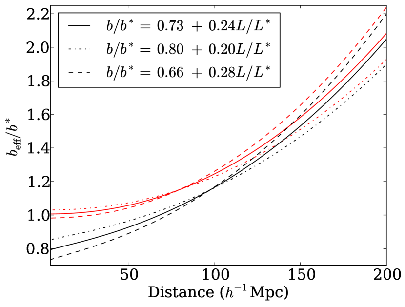
Using the functional form of quoted above from Westover (2007), this normalization procedure was applied to the 2M++ density contrast fields. Both the number-weighted and luminosity-weighted effective bias for , , and a magnitude limit of 12.5 are shown in Figure 3. We can then rewrite Equation (1) as
| (9) |
where we have defined , and .
2.5 Reconstruction Procedure
The weighted galaxies from 2M++ have measured redshifts , and not precise distances . However, application of (1) requires distances as opposed to redshifts. We refer to the inverse problem of determining the positions from redshifts as “reconstruction.” Reconstruction was accomplished via an iterative procedure modeled on that of Yahil et al. (1991). Objects were first grouped using the “Friends-of-friends” algorithm (Huchra & Geller, 1982), and then placed at the mean of their group redshift distance to suppress the “Fingers-of-God” effect. Gravity was then “adiabatically” turned on by increasing from 0 to 1 in steps of 0.01. The reconstruction took place in the LG frame, and on each iteration the following steps were taken:
- 1.
-
2.
Galaxies from 2MRS with distances greater than 125 Mpc are assigned a weight of zero. Galaxy properties, including newly computed weights are then cloned to account for incompleteness and fill the ZoA as described in §2.1.
-
3.
Number weighted galaxies or their weighted luminosities within 200 Mpc are then placed on a grid.
-
4.
The density constrast field is then computed and normalized to the same bias, , as described in §2.4. The field is in turn smoothed with a Gaussian kernel of width 4 Mpc.
-
5.
Using Equation (9) the density contrast field is then used to obtain predicted peculiar velocities for all objects in the catalogue.
- 6.
-
7.
The previous five predictions for a galaxy’s distance are then averaged to suppress oscillations arising from triple valued regions, i.e. regions of high-density near which there are multiple solutions for distance given redshift (discussed further in Appendix B). The averaged distance is in turn assigned to the galaxy and used to recompute the galaxy’s absolute magnitude. Computed distances and magnitudes are then used in the subsequent iteration.
Catalogues containing updated distances, luminosities and weights were saved at each iteration (corresponding to increasing values of ) in addition to the computed density and velocity fields.
It should be noted that this iterative reconstruction procedure was found to be unbiased in determining the best fit value of when the full analysis was run on an N-body simulation using a CDM cosmology (see Appendix A for more details).
2.6 Cosmography
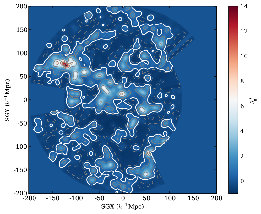
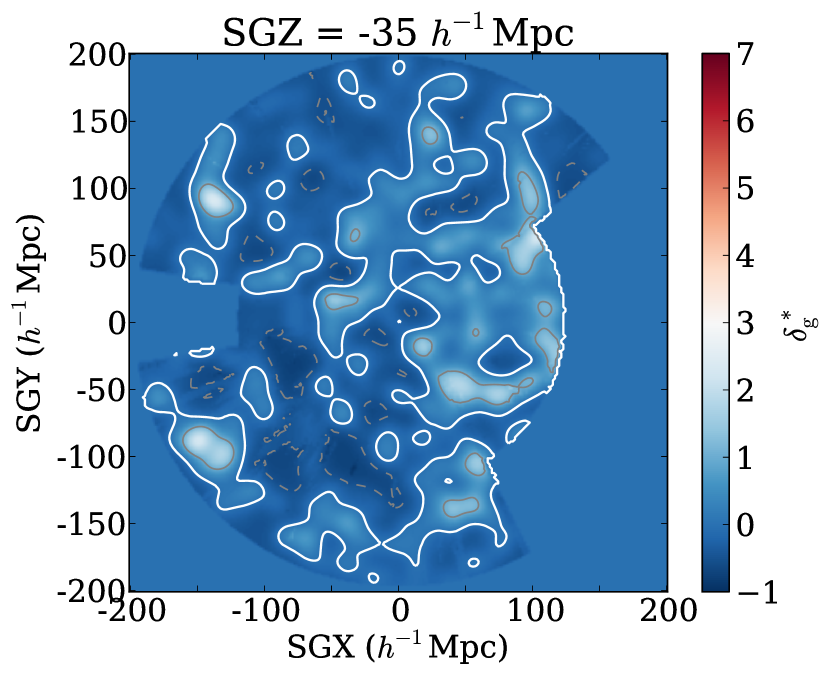
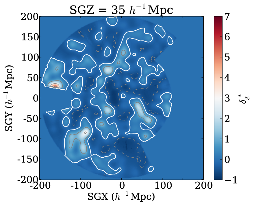
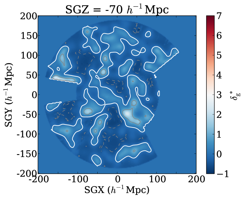
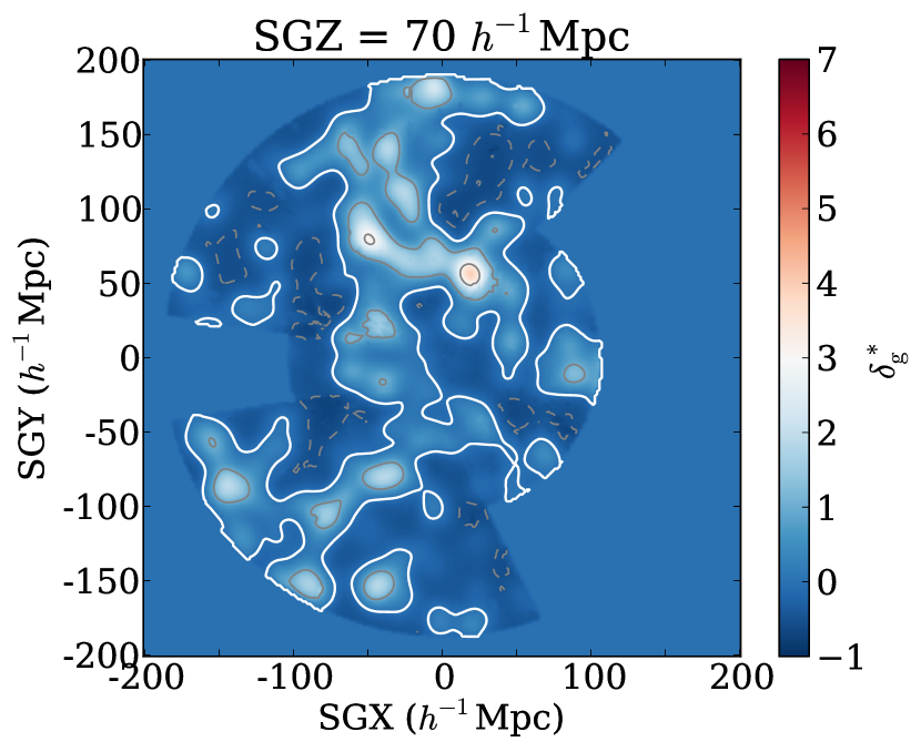
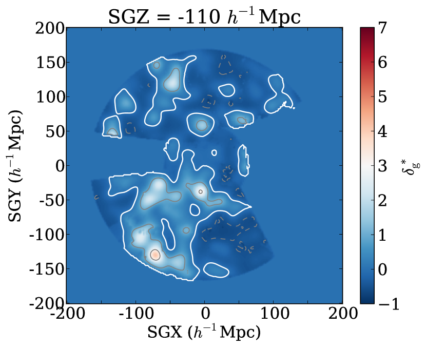
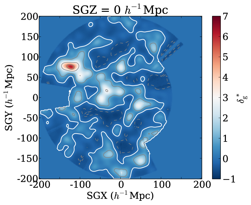
Figure 4 shows the luminosity-weighted density field of the Supergalactic Plane for , smoothed with a 4 Mpc Gaussian kernel. The incomplete coverage due to the lower magnitude limit of 2MRS is clearly visible in this figure beyond SGX 125 Mpc. The most prominent overdensity in this plane is the Shapley Concentration located at (SGX, SGY) (-125, 75) Mpc. Other notable structures in Figure 4 include the Virgo Supercluster directly above the LG, the Hydra-Centaurus Supercluster at (-40, 20) Mpc, and the Perseus-Pisces Supercluster (40, -30) Mpc. Additional slices through SGZ are shown in Figure 5, though smoothed on a 7 Mpc scale to enhance the contrast of large overdensities. For instance, Horologium-Reticulum Supercluster can be readily observed at SGZ -112 Mpc, SGX -70 Mpc, SGY -140 Mpc. The supergalactic plane is also shown with this smoothing for comparison.
3 2M++ Predicted Peculiar Velocity of the Local Group
The velocity of the LG as predicted by linear theory for an ideal distance-limited catalogue is given by:
| (10) |
where encapsulates contributions from beyond , and to first order, can be approximated as a dipole, or “residual” bulk flow. For a realistic flux-limited catalogue, we do not detect a continuous distribution of matter but a finite number of galaxies. As a result, our estimate of the velocity of the LG using 2M++ is subject to shot noise. To estimate the effect of shot noise on our predicted motion of the LG, we computed the standard deviation in each of the components of 500 bootstrap samples. The shot noise in the amplitude of the LG’s motion from this analysis was found to be 56 km s-1.
Under the assumption that the observed CMB dipole arises from the motion of the LG, there has been much debate as to the structures sourcing this motion. Most recent work has made use of 2MASS-XSC or 2MRS in reconstructing the motion of the LG, and there has yet to be consensus on the distance at which the LG’s motion coincides with that derived from the CMB. Erdoǧdu et al. (2006) argue that more than 70% of the LG’s motion results from structures within 50 Mpc, such as Hydra-Centaurus Supercluster. While others argue for convergence at distances greater than 120 Mpc such as Lavaux et al. (2010) using Monge-Ampère-Kantorovich orbit-reconstruction method, or Bilicki et al. (2011), who explored the convergence of the 2MASS dipole moment of the angular distribution of galaxies as a function of the limiting flux of the sample. As 2M++ is a superset of 2MRS and contains redshift measurements up to a magnitude limit of , this data is well suited to examine the influence of structures beyond 120 Mpc on the velocity of the Local Group.
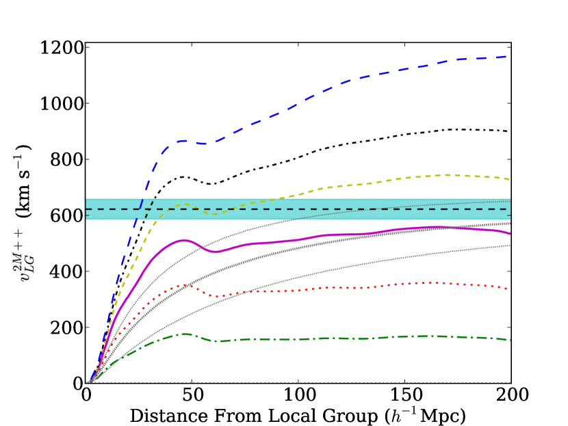
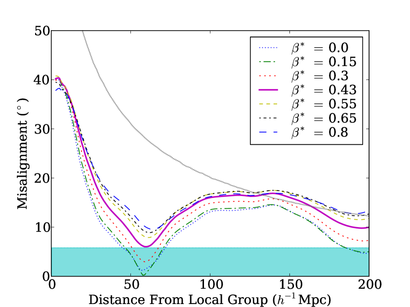
Using density fields for different values of that were obtained throughout the iteration procedure discussed in §2.5, the velocity field of increasingly larger concentric spheres centered on the LG was computed. The direction and amplitude of the LG velocity as a function of distance for different values of was then obtained. The amplitude of the LG velocity as predicted by 2M++ for different values of is shown in Figure 6a. The expected agreement between predictions using linear theory for a survey of a certain depth with values derived from the CMB are plotted for comparison. This conditional probability assumes a CDM WMAP9 cosmology. A derivation of this conditional velocity can be found in Appendix A of Lavaux et al. (2010), and is based on Lahav et al. (1990). The convergence of the direction of LG velocity with that derived from the CMB (, ) is plotted in Figure 6b. For our best fit value of from §4 below, the misalignment is . This misalignment angle is significantly better than those found by past studies using the shallower 2MRS, such as the misalignment found by Erdoğdu et al. (2006), found by Bilicki et al. (2011), or the misalignment found by Lavaux et al. (2010).
4 Peculiar Velocity Comparisons
In principle it is possible to constrain cosmological parameters by comparing the growth of predicted motion of the LG with its observed motion. This is difficult in practice because one expects contributions from sources beyond the survey limit, which we have modeled here as a residual dipole . There is therefore a degeneracy between and parameters appearing in equation (10). Very early studies of the growth of the LG gravity dipole observed the flatness at large radii from data similar to that shown in Figure 6, therefore assumed that was negligible, and hence solved for . This procedure, however, leads to a value of which is biased high, since and the integral in (10) are correlated. An alternative approach is to constrain by assuming a cosmological model of density fluctuations, but this then makes the exercise model-dependent.
A better approach is to break the degeneracy by measuring peculiar velocities of galaxies or groups other than the LG. In this section, we discuss comparisons between the predicted and observed motions of two samples of galaxies, derived from the Tully-Fisher (TF) relation and from Type Ia supernovae.
4.1 Peculiar Velocity Surveys
4.1.1 SFI++
SFI++ (Springob et al. 2007) builds primarily on Spiral Cluster I-band (SCI) and Spiral Field I-band (SFI) samples and uses a mixture of 21-cm line profile widths and optical rotation curves in determining the I-band Tully-Fisher (TF) relation from a subset of 807 galaxies in the fields of 31 clusters and groups Masters et al. (2006). From the derived TF relation they in turn determine the peculiar velocities of 5780 galaxies. Upon removing galaxies without high-quality width measurements and those that are located beyond the volume covered by 2M++, SFI++ can be divided in to two subsets of 2583 field galaxies and 735 galaxy groups.
As noted by Davis et al. (2011), the SFI++ TF relation has a kink in the faint end (), and an asymmetric distribution of outliers about the expected velocity width parameter (Springob et al. 2007). As we will be fitting for the inverse TF relation, we will account for the outliers and deviation from linearity of the relation by excluding galaxies with redshift-distance magnitudes fainter than -20. We then iteratively compute the TF relation parameters and remove those with a velocity width that deviates by more than 0.2 in (3.8) from the relation, until derived parameter values converge. Selection on both magnitude and velocity width resulted in the rejection of 503 field galaxies and 137 galaxy groups. Furthermore, when comparing predicted velocities from 2M++ with those from SFI++, the remaining objects which were found to differ by more than 3.5 with all velocity fields obtained through the reconstruction procedure were rejected (0.6%). The final sample was composed of 2067 field galaxies and 595 galaxy groups. The typical or characteristic depth of the sample can be quantified by a weighted mean distance, where the weights are the inverse square of the uncertainties. This yields depths of of 42 Mpc and 25 Mpc for field and group samples respectively.
For the TF relation, we will perform the fit two different ways. The first is a direct maximum-likelihood fit to the observed linewidths: the VELMOD method of Willick et al. (1997), as described in Section 4.2.1 below. The second method uses the estimated distances as given by Springob et al. (2007), but corrected for the fact that their peculiar velocities were obtained under the assumption that . Specifically, we use the analytic relation from Equation (2) to obtain velocities from measured positions.
4.1.2 First Amendment Supernovae
The First Amendment (A1) catalogue Type Ia Supernovae (SNe) datasets compiled by Turnbull et al. (2012). A1 is composed of SNe within 200 Mpc and draws 34 SNe from Jha et al. (2007), 185 from Hicken et al. (2009) and 26 from Folatelli et al. (2010). Of these 245 SNe, 237 are within the volume spanned by 2M++, and have an uncertainty-weighted depth of 31 Mpc.
4.2 Velocity-Velocity Comparisons
For the SFI++ subsets we use the distances as determined in Springob et al. (2007) which have not been corrected for Malmquist bias. We similarly do not use Malmquist bias corrected A1 distances. Of the comparison methods discussed below, VELMOD is unaffected by inhomogeneous Malmquist bias, and accounts for homogeneous Malmquist bias in the likelihoods. The Forward Likelihood method discussed accounts for both homogeneous and inhomogeneous Malmquist bias in the likelihoods. The simple comparison, however, neither accounts for homogeneous nor inhomogeneous Malmquist bias, and as such, the results yielded from this analysis are taken to be biased.
4.2.1 VELMOD
VELMOD is a rigorous maximum likelihood method first proposed and implemented by Willick et al. (1997) and described further in Willick & Strauss (1998). It is a velocity-velocity comparison method used to fit for the TF relation parameters (zero-point, slope and scatter) while simultaneously fitting for . VELMOD takes as inputs TF parameters, an object’s redshift and one of the observables (velocity-width or apparent magnitude), and maximizes the probability of observing one given the other. The strength of VELMOD analysis is that it neither assumes a one to one mapping from redshift space to real space (accounting for errors due to triple-valued regions), nor does it require calibration of the TF relation prior to its implementation.
Forward VELMOD uses the velocity-width to predict a galaxy’s apparent magnitude, whereas the inverse method uses the apparent magnitude to predict the velocity-width parameter. The forward method is strongly dependent on selection effects, and thus requires a well-modeled selection function. The inverse method, however, is much less sensitive to selection effects due to sample selection’s possible weak dependence on velocity-width. As the selection function of SFI++ is rather difficult to model accurately due to its being a compilation of various surveys with a range of selection criteria, we will make use of the inverse method in our analysis. This analysis assumes a TF relation of the form , where , is the absolute magnitude, is the luminosity distance, and where , and are the slope, intercept and rms scatter of the inverse relation, respectively.
The conditional probability of observing a measured velocity-width of a galaxy with an apparent magnitude, , and an observed redshift, , is given by:
| (11) |
where
| (12) |
| (13) |
| (14) |
| (15) |
where is related to the comoving distance through Equation (3), is the selection function, is the radial predicted velocity scaled to , is the scatter in the actual velocity compared to the linear theory prediction, and where is the distance modulus. We take based on the tests discussed in Appendix A. We can then compute the product of the conditional probability over all galaxies and minimize the quantity
| (16) |
for the parameters , , , and the three components of .
4.2.2 Forward Likelihood
We use a maximum likelihood method first described in Pike & Hudson (2005) which was developed to compare peculiar velocities obtained through SNe surveys while accounting for triple-valued regions. In addition to constraining and the three components of this method can be used to constrain , a nusiance parameter which permits a rescaling of published distances. The forward likelihood method maximizes the probability of a galaxy having its observed redshift
| (17) |
where
| (18) |
| (19) |
where is given through the relation
| (20) |
and where
| (21) |
is the distance as determined by the peculiar velocity survey, and where is the uncertainty is the measured distance. The product of for all objects is then computed, from which the quantity is minimized.
4.2.3 Minimization
In addition to the comparison method discussed above we also perform a simple minimization procedure to determine the best value of and . For this minimization procedure we compare the observed redshift of the object with the sum of its measured distance and predicted peculiar velocity at that distance, i.e.
| (22) |
where is given by Equation (19). Note that this expression does not account for the effects of density inhomogeneities along the line of sight. The recovered value of is affected by inhomogeneous Malmquist bias and results from this method are thus expected to be biased high as a result. Nevertheless, the statistic is useful to assess goodness-of-fit and so is included here.
4.3 Results
Key results obtained through velocity-velocity comparison methods discussed in §4.2 are summarized in Table 1. To determine the value of at which and are minimized, a cubic function was fit to resultant data. Comparison of the TF relation constants (, ) obtained to those found by Masters et al. (2006) are shown in Table 2. The best fit value for all parameters, including and its errors were obtained from 500 bootstrap samples of both 2M++ and the peculiar velocity datasets. Through bootstrap analysis it was found that peculiar velocity datasets and 2M++ contributed essentially equal amounts to overall parameter errors. The value obtained for the best fit residual bulk flow, , is given in Table 3 along with the bulk flow (50 Mpc Gaussian-weighted mean of the velocity field) and the predicted velocity of the LG arising from 2M++. A comparison of with and without the residual bulk flow results in a difference of 34 for the 3 degrees of freedom, the residual bulk flow model is thus preferred at the 5.1 level.
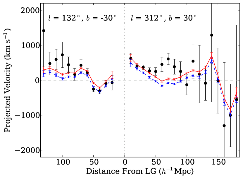
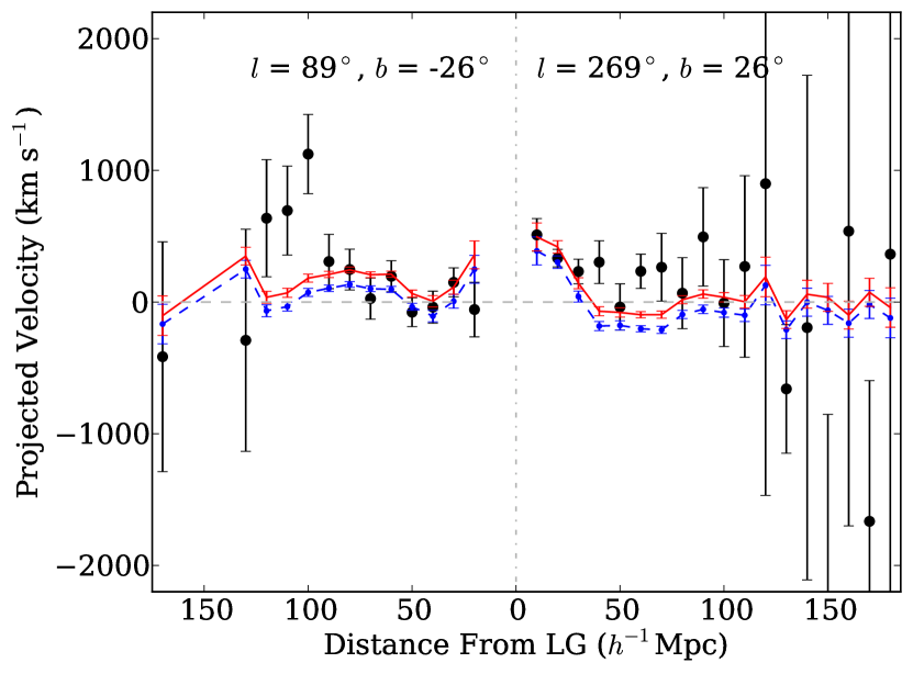
For a qualitative illustration of the agreement of predicted velocities arising from 2M++ with the published values from SFI++ and A1 we have plotted the projected line-of-sight (LOS) velocity within a cone centered on the Shapley Supercluster and Hydra Supercluster in Figure 7. These two structures were chosen as they lie in approximately the same direction as . From this figure it is apparent that predictions do in fact follow the trends observed in measured velocities. Furthermore, it is apparent that addition of to predicted velocities seems to provide better agreement, suggesting that such a residual bulk flow is in fact warranted.
In combination with a measurement of , can be used to constrain the cosmology dependent (and survey independent) degenerate parameter combination . To measure from 2M++ we follow a similar prescription to that of Efstathiou et al. (1990), we compute using counts in cells within radial shells. Using this maximum likelihood scheme we obtain the value , where the errors quoted are derived from the scatter among different shells, as this value was found to be more conservative then the formal errors from the likelihood analysis. This value is in good agreement with that found by Westover (2007) of obtained by fitting projected correlation functions to 2MRS galaxies within the magnitude range containing galaxies, i.e. . The product of the growth factor and non-linear is thus . By adopting the value of , we can transform our non-linear value of to a linearized value following the prescription of Juszkiewicz et al. (2010). We in turn obtain the constraint . It is important to note that linearization is only weakly dependent on the adopted value of ( results in ). We compare these results with those obtained using independent methods in the following section.
| (D.O.F.) | ||
|---|---|---|
| Forward Likelihood (LW) | ||
| A1 | 0.440 0.023 | - |
| SFI++ Galaxy Groups | 0.429 0.022 | - |
| SFI++ Field Galaxies | 0.423 0.045 | - |
| All | - | |
| Forward Likelihood (NW) | 0.439 0.020 | - |
| Inverse VELMOD (LW) | 0.387 0.048 | - |
| (LW) | 0.444 0.026 | 2194/2899 |
| (NW) | 0.442 0.028 | 2200/2899 |
| Masters et al. (2006) | -20.881 | -8.435 |
|---|---|---|
| This Study | -20.918 0.012 | -8.19 0.06 |
| (km s-1) | (km s-1) | (km s-1) | (km s-1) | longitude (∘) | latitude (∘) | |
|---|---|---|---|---|---|---|
| BF2M++ | -3 8 | -72 11 | 38 11 | 81 11 | 268 6 | 28 10 |
| LG2M++ | -18 27 | -422 41 | 328 37 | 535 40 | 268 4 | 38 6 |
| 89 21 | -131 23 | 17 26 | 159 23 | 304 11 | 6 13 | |
| BF2M++ + | 86 22 | -203 26 | 55 28 | 227 25 | 293 8 | 14 10 |
| LG2M++ + | 71 34 | -553 47 | 345 46 | 656 47 | 277 4 | 32 6 |
5 Discussion
5.1 Potential Systematic Effects
In this section we discuss the various effects which could bias our measurement of and our prediction of the motion of the LG. Possible contributing factors include:
-
1.
Choice of smoothing length used for Gaussian kernel may skew our estimate of .
-
2.
Non-linear contributions to velocities from nearby small scale structure may systematically bias results.
-
3.
Triple valued regions may result in incorrectly reconstructed galaxy positions skewing velocity predictions derived therefrom.
-
4.
As the reconstruction is being done in the LG frame, at each iteration we are subtracting the motion of the LG from all galaxies, our procedure may thus be susceptible to the Kaiser rocket effect.
-
5.
Sparseness of survey may result in an under-representation of structures within the survey volume.
-
6.
Structures which lie in the ZoA are not included in 2M++ and could contribute to the direction and amplitude of the motion of the LG as well as influencing predictions of peculiar velocities of galaxies near the galactic plane.
-
7.
A non-linear relation between mass and luminosity as well as scatter in the underlying relation may influence predictions.
We have addressed some of these concerns above, but will review them again here for completeness.
In addressing (i), the width of the Gaussian kernel was chosen to be 4 Mpc as this length was shown to be least biased when velocity predictions were compared to those derived from simulations. Furthermore, this smoothing length was found to produce minimal scatter in the derived relation. We have accounted for (ii) and by performing the full reconstruction and analysis on data derived from N-body simulations. It was found that a value of km s-1 should be used for the scatter around predictions to account for these effects. As for (iii), we used maximum likelihood methods which integrate likelihoods along the line-of-sight. As these methods account for uncertainty in a galaxy’s position, results should not be sensitive to a misallocation of a galaxy in the event that it is lies within a triple-valued region. The value of derived from this analysis was found to be unbiased when performed on simulations. A more complete discussion of the quantification of these systematics through analysis of N-body simulations can be found in Appendix A.
As seen in Figure 6 although the direction of the LG is not very susceptible to the value of , the overall amplitude varies by 1200 km s-1 between and . As we are doing the reconstruction in the LG frame, an error in the estimate of the motion of the LG may result in spurious distance estimates of objects along this line of motion. Putting objects at the incorrect distance may in turn result in incorrect object weights, and in turn, incorrect velocity predictions. This phenomenon has come to be known as the Kaiser “Rocket Effect”, as it was first discussed in Kaiser (1987). To account for this effect Strauss et al. (1992) explored a “Kaiser Fix” to the IRAS 1.2 Jy sample. This “fix” amounts to altering the predicted distances of objects to
| (23) |
where is the velocity of the LG as inferred from the CMB dipole, and where is 1,000 km s-1 as determined by the observed velocity correlation function (Bertschinger et al., 1990). Note that this fix assumes that galaxies more distant than are in fact at rest in the CMB frame, which may not be the case; indeed our data suggests otherwise. Nevertheless, to estimate the sensitivity of our results to this effect, we have implemented the Kaiser fix. We find that the final estimate of differs by only 3%, which is small compared to the random errors.
The impact of survey sparseness on the methodology applied in this work has been estimated in the past by Pike & Hudson (2005). For the 2MASS catalogue they found that under-sampling by 50% produced negligible results on their final estimate of (2-3%). Furthermore, we have accounted for the effects of sparse sampling by obtaining our quoted results and errors from bootstrap resampling of both 2M++ and peculiar velocity datasets. In addressing (vi) we measured at high latitudes () and found no deviation from previous results beyond that of the random errors.
When the density field was normalized to the same bias, number-weighting and luminosity-weighting schemes yielded consistent results. As the was found to be smaller for the luminosity weighted result than that obtained with number weighting, we hereafter will be quoting the best value of as that obtained from the luminosity weighting scheme. Results obtained in this paper account for neither a non-linear relation between mass and luminosity, nor do they account for scatter in mass-luminosity relation. More sophisticated models have been proposed, such as the halo-model of Marinoni & Hudson (2002), and recently an iterative prescription to reconstruct the density field from the distribution of halos (Wang et al., 2009). We will consider implementation of such methods in a future paper.
5.2 Comparison With Other Results
As the bias depends on luminosity and possibly morphology (cf. Pike & Hudson 2005), the value of obtained is survey dependent. As 2M++ draws primarily from 2MASS, however, a loose comparison can be made with other values of obtained therefrom. Most recently, in comparing the clustering dipole of galaxies from 2MASS-XSC to predictions from linear theory assuming a CDM cosmology and convergence of the LG dipole with that derived from the CMB, Bilicki et al. (2011) found . After constructing dependent predictions of peculiar velocities, Branchini et al. (2012) in turn estimate by minimizing the scatter of predicted 2MASS absolute magnitudes about a universal luminosity function and find . Davis et al. (2011) expand the velocity field in spherical harmonics and fit the inverse TF relation to SFI++ finding . The TF data span a range of distances, and because the effective bias changes with distance it is difficult to compare this directly with our number-weighted result . The characteristic, or error-weighted, depth of all individual SFI++ galaxies is . At this distance, the typical relative bias of a number-weighted sample with the magnitude limit of 2MRS is , and so applying this to the Davis et al. (2011) result yields
Our value of is in good agreement with those obtained using the same methodology, such as that of Turnbull et al. (2012) (), that of Pike & Hudson (2005) (), as well as with the weighted IRAS average of multiple studies reported therein (). As noted above, it is, however, in slight tension with that found by Davis et al. (2011) (). Note that where necessary the values quoted here have been linearized following the procedure discussed above in §4.3.
5.3 Cosmological Implications
5.3.1 The value of
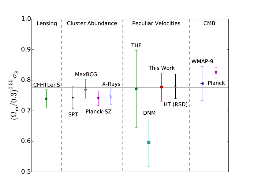
We can also compare our value to constraints placed on a degenerate combination of and through independent means. In particular our value is in excellent agreement with a different peculiar velocity probe, namely measurements of at different redshifts via redshift space distortions, which yield a best-fit value of (Hudson & Turnbull, 2012).
An analysis of second and third-order weak-lensing aperture-mass moments measured by CFHTLenS yields (Kilbinger et al., 2013). Constraints can also be obtained from the number counts and mass of galaxy clusters as measured through X-ray surface brightness (Vikhlinin et al. 2009) and measurements of the Sunyaev-Zeldovich (SZ) effect (Planck Collaboration et al. 2013a, Reichardt et al. 2013). Finally, we can obtain a value for from CMB temperature anisotropy from Planck ( ; Planck Collaboration et al., 2015) and WMAP9 ( ; Hinshaw et al., 2013). The measurements use different methods and are at different redshifts, and so their dependence on differs in the exponent. To make a quantitative comparisons between different results, we adopt (see Figure 8). There is some tension between some results e.g. Kilbinger et al. (2013) and Planck-SZ (Planck Collaboration et al., 2013a) versus Planck CMB temperature (Planck Collaboration et al., 2015). The peculiar velocity result presented here is consistent with all of these values.
5.3.2 The motion of the LG
For our best value of we can compare the predicted growth of the LG velocity amplitude with the result that one would expect to measure using linear theory for a CDM cosmology (conditional on ). For 0.431 0.021, as determined from peculiar velocity comparisons, we obtain the prediction for the motion of the Local Group arising from 2M++ to be 535 40 km s-1 in the direction , , only out of alignment with the direction of the motion as inferred from the CMB dipole. The residual LG motion is therefore 100 37 km s-1 in the direction , . This value is in reasonable agreement with the best fit residual bulk flow obtained through peculiar velocity comparisons in the CMB frame of 159 23 km s-1 in the direction , . Inclusion of this residual bulk flow with the predicted motion of the LG arising from 2M++ results in a total predicted motion of 656 47 km s-1 in the direction , , in even better agreement with both the amplitude and direction of the motion as inferred from the temperature dipole of the CMB.
5.3.3 The residual bulk flow
We find that the amplitudes and directions of fit to each of the SFI++ and A1 SNe datasets separately are consistent with one another. Furthermore, comparing A1 with PSCz (of comparable depth to 2M++), Turnbull et al. (2012) found a residual flow of km s-1, km s-1, km s-1, in reasonable agreement with the values found here of km s-1, km s-1, km s-1. This suggests that the residual bulk flow is not an artifact of either the analysis or redshift-catalogue and is sourced by structures outside the 2M++ and PSCz volumes.
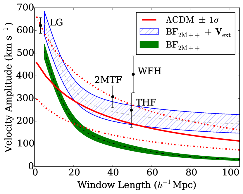
We can also use the 2M++ density field to predict the BF and compare this to the BF expected in a CDM universe in Figure 9. We have plotted this comparison for the Gaussian-weighted mean of the 2M++ velocity field. It is apparent from this figure that the resulting bulk flow from our analysis is in agreement with that expected for a CDM universe. Combining the cosmic variance in quadrature with observational errors, comparison of the measured bulk flow of a 100 Mpc Gaussian with predictions from CDM yield a of 1.4 for 3 degrees of freedom; clearly the measured value agrees well with the predicted value from the standard cosmological model.
5.3.4 A large-scale underdensity?
There have been recent claims that the Local Universe (150–200 Mpc) is under-dense (Whitbourn & Shanks 2013, Keenan et al. 2013). Such a phenomenon might account for the discrepancy between the larger value for the Hubble parameter when measured locally () and that obtained from studies of the CMB temperature anisotropies.
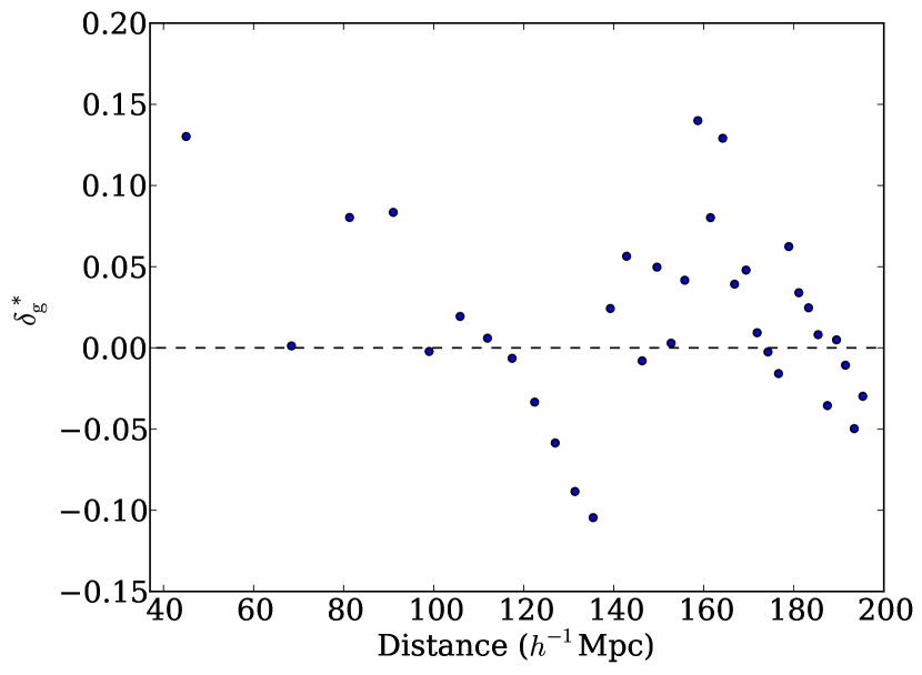
Although the majority of 2M++ lies within the suggested underdensity, we have nonetheless explored the possibility of a under-dense volume within 2M++. The luminosity-weighted density contrast of 2M++ in shells is shown in Figure 10. We have not observed any global systematic rise in density towards the periphery of the survey.
To compare our results with others in more detail, note that Whitbourn & Shanks (2013) use redshift data from three large regions: 6dF-SGC, 6dF-NGC & SDSS-NGC. Within , they quote mean density contrast of , and , respectively. For the same volumes, we find density contrasts of , and respectively, where the density is normalized with respect to the mean density within 200 Mpc (). Boehringer et al. (2014) studied the large-scale densities of X-ray clusters. For the 6dF-SGC and 6dF-NGC regions, they find mean cluster density contrast of and within . However, as they point out, galaxy clusters are highly biased () and so the corresponding mean matter density contrasts are and . These latter numbers are in good agreement with our nearly-unbiased galaxy luminosity results. We conclude that, while the 6dF-SGC region may be mildly underdense within , there is no evidence for a large-scale void.
5.3.5 Prospects for the future
There are several upcoming peculiar velocity surveys which should dramatically improve the constraints on both and . Among these is the survey dubbed “Transforming Astronomical Imaging surveys through Polychromatic Analysis of Nebulae” (TAIPAN). Using the UK Schmidt telescope, it is estimated that TAIPAN will acquire 45,000 Fundamental-Plane velocity measurements out to a redshift of 0.2 (Koda et al. 2013). The next generation of Tully-Fisher (TF) peculiar velocity surveys include the Widefield ASKAP L-band Legacy All-sky Blind surveY (WALLABY, Koribalski & Staveley-Smith 2009), and the Westerbork Northern Sky HI Survey (WNSHS)111http://www.astron.nl/jozsa/wnshs/. An HI survey acquired using the Australian Square Kilometer Array Pathfinder (ASKAP), WALLABY is planned to cover 3 steradian of sky. Its Northern Hemisphere counterpart, WNSHS, is planned to cover remaining steradian of the sky using the Westerbork Synthesis Radio. It is estimated that these surveys will obtain a total of 32,000 velocity measurements, and along with TAIPAN will not only enable -dependent measurements of but will improve constraints on this parameter combination at low-redshift () to within 3% (Koda et al. 2013). Clearly constraints on cosmology through peculiar velocities has a very promising future.
6 Conclusion
Under the assumption of gravitational instability, we reconstructed the galaxy density field within 200 Mpc using 2M++, a composite all-sky redshift redshift survey with high completeness. We compared the predicted peculiar velocities arising from this density field to the measured peculiar velocities of SFI++ and the First Amendment supernovae dataset using various comparison methods in order to measure . Using the VELMOD maximum likelihood comparison method with SFI++ spiral galaxies we simultaneously solved for the inverse TF relation zeropoint and slope, , as well as a residual bulk flow due to sources external to the 2M++ volume, denoted . We similarly compared peculiar velocities datasets to predictions from 2M++ using a forward-likelihood method in order to constrain and . All methods and data subsets yielded consistent values of , with our final result being 0.431 0.021. Combining our value of with as measured from 2M++ for 0.43, we in turn measured the parameter combination 0.401 0.024. This value was found to be consistent with the majority of results obtained by independent means, including those of WMAP9 and Planck.
For our measured value of we computed the velocity of the Local Group as predicted by linear theory arising from the reconstructed density field. Our value for the velocity was found to be consistent with the theoretical value that would be measured for a survey of this depth in a CDM Universe. Combining our predicted value for the motion of LG arising from 2M++ for our best value of with the value of obtained through comparing predicted velocities with peculiar-velocity surveys, we predict a motion of the LG to be km s-1, towards , , only 5∘ out of alignment with the direction as inferred from the CMB dipole. Similarly, with addition of this residual bulk flow to the 50 Mpc Gaussian-weighted mean of the velocity field, we obtained a predicted bulk-flow of km s-1 towards , , an amplitude that is consistent with that expected for a CDM Universe. We note, however, that although we find the inclusion of is preferred at the 5.1 level, it is unclear whether this residual bulk flow merely compensates for imperfect mapping between luminosity and mass towards the periphery of 2M++, or whether it is due to structures outside the 2M++ volume. Future work using more sophisticated biasing schemes may help in answering this question.
The resulting 2M++ density and peculiar velocity fields obtained from this analysis are made available at cosmicflows.uwaterloo.ca and cosmicflows.iap.fr .
7 Acknowledgements
All authors acknowledge support from the Natural Sciences and Engineering Council of Canada. This work made in the ILP LABEX (under reference ANR-10-LABX-63) was supported by French state funds managed by the ANR within the Investissements d’Avenir programme under reference ANR-11-IDEX-0004-02.
References
- Abazajian et al. (2009) Abazajian K. N. et al., 2009, ApJS, 182, 543
- Behroozi et al. (2013) Behroozi P. S., Wechsler R. H., Wu H.-Y., 2013, ApJ, 762, 109
- Berlind et al. (2000) Berlind A. A., Narayanan V. K., Weinberg D. H., 2000, ApJ, 537, 537
- Bertschinger et al. (1990) Bertschinger E., Gorski K. M., Dekel A., 1990, Nature, 345, 507
- Bilicki et al. (2011) Bilicki M., Chodorowski M., Jarrett T., Mamon G. A., 2011, ApJ, 741, 31
- Bilicki et al. (2011) Bilicki M., Chodorowski M., Mamon G. A., Jarrett T., 2011, ApJ, 741, 31
- Blanton et al. (2005) Blanton M. R. et al., 2005, AJ, 129, 2562
- Boehringer et al. (2014) Boehringer H., Chon G., Bristow M., Collins C. A., 2014, ArXiv e-prints
- Branchini et al. (2012) Branchini E., Davis M., Nusser A., 2012, MNRAS, 424, 472
- Courteau & van den Bergh (1999) Courteau S., van den Bergh S., 1999, AJ, 118, 337
- Davis & Huchra (1982) Davis M., Huchra J., 1982, ApJ, 254, 437
- Davis et al. (2011) Davis M., Nusser A., Masters K. L., Springob C., Huchra J. P., Lemson G., 2011, MNRAS, 413, 2906
- Efstathiou et al. (1990) Efstathiou G., Kaiser N., Saunders W., Lawrence A., Rowan-Robinson M., Ellis R. S., Frenk C. S., 1990, MNRAS, 247, 10P
- Erdoğdu et al. (2006) Erdoğdu P. et al., 2006, MNRAS, 368, 1515
- Erdoǧdu et al. (2006) Erdoǧdu P. et al., 2006, MNRAS, 373, 45
- Folatelli et al. (2010) Folatelli G., Phillips M. M., Burns C. R., Contreras C., 2010, AJ, 139, 120
- Hicken et al. (2009) Hicken M., Wood-Vasey W. M., Blondin S., Challis P., Jha S., Kelly P. L., Rest A., Kirshner R. P., 2009, ApJ, 700, 1097
- Hinshaw et al. (2013) Hinshaw G. et al., 2013, ApJS, 208, 19
- Hinshaw et al. (2009) Hinshaw G. et al., 2009, ApJS, 180, 225
- Hong et al. (2014) Hong T. et al., 2014, MNRAS, 445, 402
- Huchra & Geller (1982) Huchra J. P., Geller M. J., 1982, ApJ, 257, 423
- Huchra et al. (2012) Huchra J. P. et al., 2012, ApJS, 199, 26
- Hudson & Turnbull (2012) Hudson M. J., Turnbull S. J., 2012, ApJL, 751, L30
- Jha et al. (2007) Jha S., Riess A. G., Kirshner R. P., 2007, ApJ, 659, 122
- Jones et al. (2009) Jones D. H. et al., 2009, MNRAS, 399, 683
- Juszkiewicz et al. (2010) Juszkiewicz R., Feldman H. A., Fry J. N., Jaffe A. H., 2010, JCAP, 2, 21
- Kaiser (1987) Kaiser N., 1987, MNRAS, 227, 1
- Keenan et al. (2013) Keenan R. C., Barger A. J., Cowie L. L., 2013, ApJ, 775, 62
- Kilbinger et al. (2013) Kilbinger M., Fu L., Heymans C., Simpson F., Benjamin J., Erben T., Harnois-Deraps, 2013, MNRAS, 430, 735
- Koda et al. (2013) Koda J. et al., 2013, ArXiv e-prints
- Koribalski & Staveley-Smith (2009) Koribalski B., Staveley-Smith L., 2009, ASKAP Survey Science Proposal
- Lahav et al. (1990) Lahav O., Kaiser N., Hoffman Y., 1990, ApJ, 352, 448
- Lavaux & Hudson (2011) Lavaux G., Hudson M. J., 2011, MNRAS, 416, 2840
- Lavaux et al. (2010) Lavaux G., Tully R. B., Mohayaee R., Colombi S., 2010, ApJ, 709, 483
- Marinoni & Hudson (2002) Marinoni C., Hudson M. J., 2002, ApJ, 569, 101
- Masters et al. (2006) Masters K. L., Springob C. M., Haynes M. P., Giovanelli R., 2006, ApJ, 653, 861
- Norberg et al. (2001) Norberg P. et al., 2001, MNRAS, 328, 64
- Peebles (1993) Peebles P. J. E., 1993, Principles of Physical Cosmology. Princeton University Press
- Pike & Hudson (2005) Pike R. W., Hudson M. J., 2005, ApJ, 635, 11
- Planck Collaboration et al. (2013a) Planck Collaboration et al., 2013a, ArXiv e-prints
- Planck Collaboration et al. (2015) Planck Collaboration et al., 2015, ArXiv e-prints
- Planck Collaboration et al. (2013b) Planck Collaboration et al., 2013b, ArXiv e-prints
- Reichardt et al. (2013) Reichardt C. L. et al., 2013, ApJ, 763, 127
- Rozo et al. (2010) Rozo E. et al., 2010, ApJ, 708, 645
- Saunders et al. (2000) Saunders W. et al., 2000, MNRAS, 317, 55
- Schechter (1976) Schechter P., 1976, ApJ, 203, 297
- Skrutskie et al. (2006) Skrutskie M. F. et al., 2006, AJ, 131, 1163
- Springel (2005) Springel V., 2005, MNRAS, 364, 1105
- Springob et al. (2007) Springob C. M., Masters K. L., Haynes M. P., Giovanelli R., Marinoni C., 2007, ApJS, 172, 599
- Strauss et al. (1992) Strauss M. A., Yahil A., Davis M., Huchra J. P., Fisher K., 1992, ApJ, 397, 395
- Tegmark et al. (2002) Tegmark M., Dodelson S., Eisenstein D. J., Narayanan V., 2002, ApJ, 571, 191
- Turnbull et al. (2012) Turnbull S. J., Hudson M. J., Feldman H. A., Hicken M., Kirshner R. P., Watkins R., 2012, MNRAS, 420, 447
- Vikhlinin et al. (2009) Vikhlinin A. et al., 2009, ApJ, 692, 1060
- Wang et al. (2009) Wang H., Mo H. J., Jing Y. P., Guo Y., van den Bosch F. C., Yang X., 2009, MNRAS, 394, 398
- Wang & Steinhardt (1998) Wang L., Steinhardt P. J., 1998, ApJ, 508, 483
- Watkins et al. (2009) Watkins R., Feldman H. A., Hudson M. J., 2009, MNRAS, 392, 743
- Westover (2007) Westover M., 2007, PhD dissertation, Harvard University, Department of Astronomy
- Whitbourn & Shanks (2013) Whitbourn J. R., Shanks T., 2013, MNRAS
- Willick & Strauss (1998) Willick J. A., Strauss M. A., 1998, ApJ, 507, 64
- Willick et al. (1997) Willick J. A., Strauss M. A., Dekel A., Kolatt T., 1997, ApJ, 486, 629
- Yahil et al. (1991) Yahil A., Strauss M. A., Davis M., Huchra J. P., 1991, ApJ, 372, 380
Appendix A Tests of the Reconstruction with N-body Simulations
In this Appendix, we focus on two possible sources of systematic bias in the reconstructed density and velocity fields. First, when constructing the density field from a set of point density tracers, it is necessary to smooth to obtain a continuous density field. If the smoothing length is too short, density contrasts are high and linear theory is no longer applicable. If the smoothing length is too long, then the density contrast is suppressed and velocities are underpredicted. Second, in “reconstructing” real-space positions from redshift-space, the iterative technique discussed in §3 may also introduce a systematic bias in the recovered density field and hence in the fitted value of .
A.1 Effect of smoothing
Berlind et al. (2000) used N-body simulations to show that when predicted velocities derived from smooth density fields are compared to measured (unsmoothed) velocities, the recovered value of depends on the smoothing. For Gaussian smoothing, unbiased results were obtained for a smoothing radius between 4 and 5 Mpc. It is interesting to confirm these results.
Here we use an N-body simulation of particles in a 500 Mpc periodic box using GADGET-2 (Springel 2005). The cosmological parameters of this simulation are as follows: , , , and where each particle is . From the particle positions and velocities of the simulation a halo catalogue was formed using ROCKSTAR (Behroozi et al. 2013) consisting of 693948 halos between and (between 8 and 31809 particles). Either halo or particle positions were smoothed to create a smooth halo or particle density field.
In Fig. 11 we plot both the slope of regression between smoothed predicted and N-body velocities, as well as the scatter about this relation, both as a function of smoothing scale.
For particle velocities compared with linear theory predictions from the smoothed particle density field, the slope is unbiased at a smoothing scale of 5 Mpc. The scatter is 250 km s-1. The results are similar for halos, but the scatter is significantly lower: 150 km s-1. This is because the particle velocity field is a sum of the motion of the halos themselves plus the internal motion of particles with respect to the halos. In both cases, the scatter is minimum for a smoothing scale of 4 Mpc.
A.2 Reconstructing the Halo Distances from Redshifts
With actual galaxy data, the true distances are unknown but redshifts are available. In this paper, we use an iterative reconstruction method to map a galaxy’s position from redshift space to real space. We will refer to these reconstructed coordinates as “recon-space.” In the N-body simulation, we emulate this by placing halos in redshift-space, and then iteratively reconstruct the density field, slowly increasing .
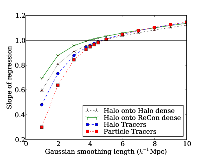
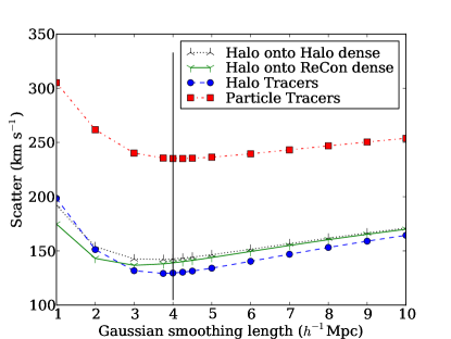
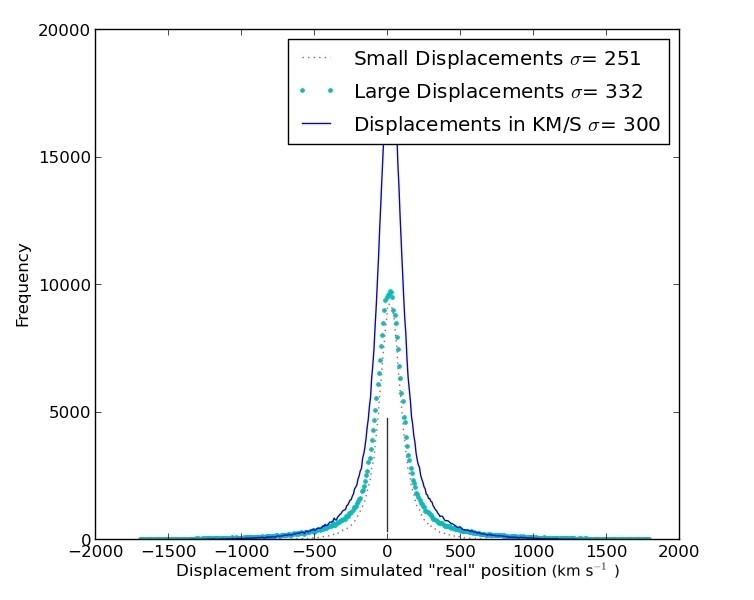
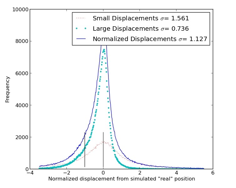
Fig. 12 shows the difference between real-space positions and recon-space positions. The left panel illustrates the absolute displacement in units of km s-1. From this panel, it is apparent that in recon-space the majority of halos do in fact return to a location close to their real-space positions, with an error that is typically km s-1. This is smaller than the smoothing scale of . However, in practice this reconstruction error will act as an additional source of smoothing. We will return to this point below.
The right panel shows the displacement of each halo from its real-space position normalized by the difference between the real-space and redshift-space positions (i.e. by their peculiar velocities). In this way the halos which lie in redshift-space have a normalized displacement of , and those which have returned to real-space have a normalized displacement of . With each successive iteration tracers would all ideally return to , i.e. return to the position they had in real-space. Halos which have a normalized displacement more negative than have moved away from their initial positions. We argue below (§B) that these are halos in triple-valued regions. From this figure it can be seen that the typical tracer does in fact return to its real-space position. However, the distinction between low and high peculiar velocity tracers is more pronounced. The tracers with a low peculiar velocity have a symmetric distribution of reconstruction error. The halos which initially have a high velocity, however, have a more skewed distribution which likely results in part from triple-valued regions.
Having reconstructed the density field in recon-space, we return to the question of how well this field, once smoothed, can predict peculiar velocities. Fig. 11 shows the results of this comparison. The fitted slope obtained from the reconstructed density field is systematically offset in comparison to those obtained from the real-space halo density field. The key result is that predicted velocities derived from the reconstructed smoothed halo fields yields an unbiased value of the slope, i.e. , when a Gaussian kernel of 4 Mpc is used. This value is smaller than the value of 5 Mpc found for halos in real-space, because the recon-space density field is effectively pre-smoothed (in the redshift direction) by the 300 km s-1 reconstruction error discussed above.
Appendix B Iterative Reconstruction Near Triple-Valued Regions
One problem with any reconstruction method is correcting for the fact that mapping from redshift to position is multivalued, i.e. there can be several distances which map to the same redshift.
To give an illustration as to how this affects the iterative reconstruction method, we have created a simple toy model in Fig. 13 which shows the velocity field around a spherical overdensity. One can see that for any object with an observed redshift in the range to , there are multiple distances that correspond to that given redshift. As a concrete example, consider a galaxy at a redshift of 300 km s-1. We will consider a simplified version of our reconstruction scheme in order to illustrate the general behaviour. In this simplified version, the value of is held fixed, i.e. it is not increased adiabatically, so the amplitude of the peculiar velocity curve is fixed and the curve is also fixed.
In the first step of this iterative process, we place the galaxy at a distance corresponding to its observed redshift: 300 km s-1 at position r(0) in Fig. 13. At this location the predicted peculiar velocity is approximately , so the object is moved to its first reconstructed position of at position r(1). At this position it has a predicted peculiar velocity of approximately , and so this predicted peculiar velocity is again subtracted from its observed redshift of 300 km s-1, resulting in a reconstructed distance of 320 km s-1indicated r(2). In this example, each successive loop brings the reconstructed position closer to the outer redshift solution of approximately 360 km s-1 indicated r(). The same behaviour occurs for redshifts between 250 and 400 km s-1, the final position converges to the third (outer) of the three values. For redshifts between 100 and 250 km s-1, in contrast, the recon position converges to the first of the three values. One can see that the outer solutions are attractors, and the middle solution is unstable.
The above toy model is for a test particle (e.g. galaxy) moving in a fixed potential well (e.g. supercluster). It can also happen that two similar-mass galaxies (or two clusters) may each respond to the other’s gravity. In this situation, the distances of the two objects can “leapfrog”, i.e. can exchange the order of their distances in reconstructed space. This leads to a sign change of the predicted peculiar velocity, which the leads to another “leapfrog” and a subsequent sign change in predicted peculiar velocity. Hence some objects show oscillatory behaviour in the reconstructed distance.
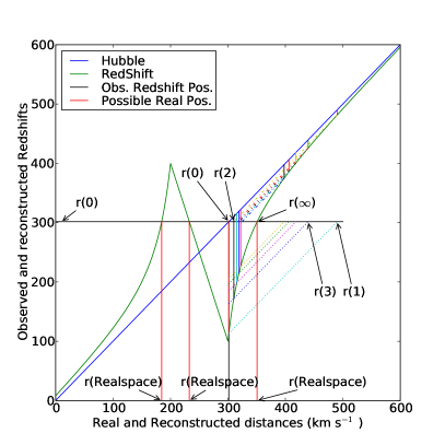
Note however that the simple model described above and in Fig. 13 is an over-simplification of our reconstruction process. Of course, while in reality the density field used is a smoothed Gaussian random sphere not a spherical top-hat overdensity, qualitatively the behaviour around overdensities is similar. More importantly, our iterative scheme is more complex than the one outlined above. First, we “adiabatically” increase at each iteration. Consequently, the amplitude of the predicted peculiar velocity field increase slowly and so the size of triple-valued regions in redshifts space grows slowly. Second, we reduce oscillatory behaviour by averaging the positions of several successive iterations. Thus the convergence is better-behaved than the toy model described above. But qualitatively, the effect remains the same: as a result of preferentially placing objects towards the periphery of triple-value regions, the density field is effectively “smoothed” more in the regions of highest density.