Level Lines of Gaussian Free Field II:
Whole-Plane
Abstract
We study the level lines of starting from interior points. We show that the level line of starting from an interior point turns out to be a sequence of level loops. The sequence of level loops satisfies “target-independent” property. All sequences of level loops starting from interior points give a tree-structure of the plane. We also introduce the continuum exploration process of starting from interior. The continuum exploration process of whole-plane satisfies “reversibility”.
1 Introduction
This is the second in a series of two papers the first of which is [WW16]. Suppose that is a smooth real-valued function defined on the complex plane , then level lines of are curves along which has constant value. In [SS09, SS13], the authors derive that one can still make sense of level lines of Gaussian Free Field (), which is nolonger a pointwise-defined function and can only be viewed as a distribution. The level lines of are still continuous curves, which are variants of Schramm Loewner Evolution ().
In [WW16], we study level lines of that start from boundary points. In the current paper, we will study level lines of that start from interior points. We show that the level line of starting from an interior point turns out to be a sequence of level loops (Theorems 1.1.1 and 1.1.2). We explain the interaction behavior between two sequences of level loops (Theorems 1.1.3 and 1.1.4): two sequences of level loops with distinct starting points but common target point will merge; two sequences of level loops with common start point and distinct target points coincide up to the first disconnecting time after which the two processes continue toward their target points in a conditionally independent way. The latter fact is so-called “target-independent” property of the sequence of level loops. Consider all sequences of level loops starting from interior points, they give a tree-structure of the complex plane (Theorem 1.1.5).
We also introduce continuum exploration processes of starting from interior points. They are sequences of quasisimple loops (Theorems 1.2.1 and 1.2.2). We describe the interaction behavior between two continuum exploration processes (Theorems 1.2.3 and 1.2.4). All continuum exploration processes starting from interior points also give a tree-structure of the plane (Theorem 1.2.5). We wish to highlight an interesting fact about the continuum exploration processes.The continuum exploration processes of whole-plane satisfy reversibility: the continuum exploration process starting from the origin targeted at “coincides” (in a certain sense which will be made precise in Theorem 1.2.6) with the continuum exploration process starting from targeted at the origin.
In a series of papers [MS16a, MS16b, MS12, MS13], the authors study the flow lines of . In particular, [MS16a] studies the flow lines starting from boundary points and [MS13] studies the flow line starting from interior points. The current paper is motivated by [MS13]. However, the situation for the level line starting from interior is quite different from the flow line case: the flow line starting from an interior point is a continuous curve; whereas, the level line starting from interior will merge with itself, and the only natural way to describe it is by a sequence of loops.
This paper is also an important part in a program on conformal invariant metric on which includes [WW13, SWW16, WW16]. In [WW13], the authors constructed a conformal invariant growing process in (recalled in Section 3.1) where each loop has a time parameter. The authors conjectured that the time parameter is a deterministic function of the loop configuration. Later, Scott Sheffield pointed out that the conformal invariant growing process in is closely related to the exploration process of (which is made precise in [WW16, Section 3] and Sections 3.2, 3.3). The tools that we develop in the current paper will be used in the program by Scott Sheffield, Samuel Watson, Wendelin Werner and Hao Wu which tries to prove the conjecture that the time parameter in constructed in [WW13] is a deterministic function of the loop configuration, and hence gives a conformal invariant metric on loops.
1.1 Sequence of level loops starting from interior
To consider level line of starting from an interior point, it is natural to consider a random sequence of level loops instead of a random path, and the height difference between two neighbor loops is for some fixed number . A simple loop in the complex plane is the image of the unit circle in the plane under a continuous injective map. In other words, a simple loop is a subset of which is homeomorphic to the unit circle . Note that a simple loop is oriented either clockwise or counterclockwise. If is a simple loop, then separates the plane into two connected components that we call its interior (the bounded one) and its exterior (the unbounded one). Assume that the origin is contained in , we define the inradius and outradius of the loop to be
We call a sequence of simple loops in the plane a transient sequence of adjacent simple loops disconnecting the origin from infinity if the sequence satisfies the following properties.
-
(1)
For each , the loop disconnects the origin from infinity;
-
(2)
For each , the loop is contained in the closure of and ;
-
(3)
The sequence is transient:
Given a transient sequence of adjacent simple loops , we use the term level loop boundary conditions with height difference to describe the boundary values given by the following rule. Assume that the loop has boundary value on the left-side and on the right-side, the boundary value of is
See Figure 1.1.1.
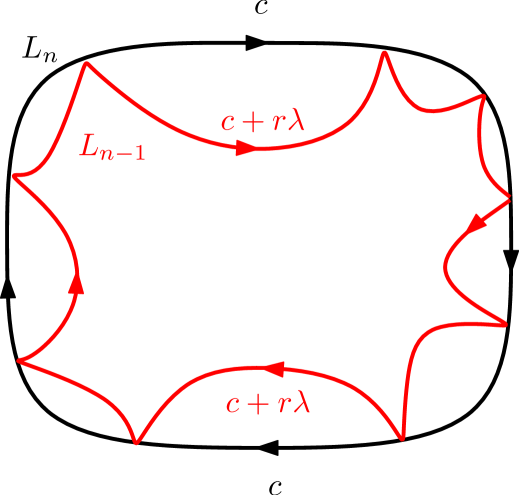
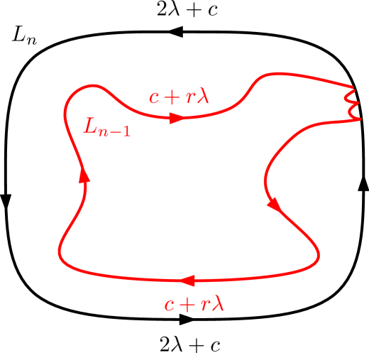
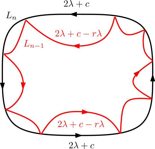
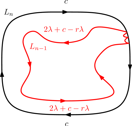
Note that, once we know the boundary values of a loop in the sequence, we can tell the boundary values of all loops , for , by the level loop boundary conditions with height difference .
We say a domain has harmonically non-trivial boundary if a Brownian motion started at a point in hits almost surely. We call a sequence of simple loops in a transient sequence of adjacent simple loops disconnecting from if the sequence satisfies the following properties.
-
(1)
For each , the loop disconnects from ;
-
(2)
For each , the loop is contained in the closure of the connected component of that contains ;
-
(3)
The sequence is transient: the loop converges to in Hausdorff metric as .
The level loop boundary conditions with height difference for a transient sequence of adjacent loops in is defined in the same way as before.
The following two theorems explain that the level line of starting from an interior point turns out to be a transient sequence of adjacent loops.
Theorem 1.1.1.
Fix a connected domain with harmonically non-trivial boundary, a starting point , and a number . Let be a on with some boundary values. There exists a coupling between and a random transient sequence of adjacent simple loops disconnecting from such that the following domain Markov property is true. For any stopping time , the conditional law of given is a GFF on whose boundary value agrees with the boundary value of on and is given by level loop boundary conditions with height difference on .
If and is a whole-plane (modulo a global additive constant in ), there is also a coupling between and a random transient sequence of adjacent simple loops disconnecting the origin from infinity such that the following domain Markov property is true. For any stopping time , the conditional law of given is a (modulo a global additive constant in ) on whose boundary value is given by level loop boundary conditions with height difference on .
Theorem 1.1.2.
In the coupling of a and a random sequence of loops as in Theorem 1.1.1, the sequence is almost surely determined by the field viewed as a distribution modulo a global additive constant in .
In the coupling between a whole-plane and a sequence of loops given by Theorem 1.1.1, we call the sequence of level loops the alternating height-varying sequence of level loops of starting from the origin targeted at .
The following two theorems explain the interaction behaviors between two sequences of level loops.
Theorem 1.1.3.
Fix . Suppose that is a whole-plane modulo a global additive constant in . Fix two starting points . For , let be the alternating height-varying sequence of level loops of with height difference starting from targeted at . Define
Then, almost surely, the loops and coincide; moreover, the two sequences of loops and coincide.
Theorem 1.1.4.
Fix . Suppose that is a whole-plane modulo a global additive constant in . Fix three points . For , let be the alternating height-varying sequence of level loops of with height difference starting from targeted at ; and denote by the connected component of that contains . Then there exists a number such that
Given , the two sequences continue towards their target points respectively in a conditionally independent way.
The following theorem explains that all sequences of level loops give a tree-structure of the plane.
Theorem 1.1.5.
Fix . Suppose that is a whole-plane modulo a global additive constant in . Suppose that is any countable dense set and, for each , let be the alternating height-varying sequence of level loops of with height difference starting from targeted at . Then the collection almost surely determines the field and its law does not depend on the choice of . Moreover, the collection forms a tree structure in the sense that, almost surely, any two sequences of level loops merge eventually.
Remark 1.1.6.
In the coupling as in Theorem 1.1.1 for , the Hausdorff dimension of the intersection of two neighbor loops is almost surely given by (see [WW16, Remark 1.1.5])
This implies that, given the sequence of level loops , we can tell the height difference through the Hausdorff dimension of the intersection of two neighbor loops.
Generally, for any two loops and in the sequence, on the event , their height difference can be read from the Hausdorff dimension of their intersection:
1.2 Continuum exploration process starting from interior
In this section, we will describe a continuum exploration process of starting from an interior point. This process can be viewed as the limit of the sequence of level loops in Theorem 1.1.1 as goes to zero.
Before defining the continuum exploration process, we need to define a suitable space of loops (see also [She09, Section 4.1]). As we introduced in Section 1.1, a simple loop is a subset of which is homeomorphic to the unit circle . Recall that is the bounded connected component of , and is a simply connected domain. There exists a conformal map from onto and can be extended as a homeomorphism from the closure of onto .


A quasisimple loop is the (oriented) boundary of a simply connected domain. Note that a quasisimple loop can be obtained as the limit of a sequence of simple loops under metric. A quasisimple loop may intersect itself, but it can not cross itself traversely. If is a quasisimple loop, we denote by the unbounded connected component of (there may be several bounded connected components of , but there is only one that is unbounded). We will say is clockwise (resp. counterclockwise) if the boundary of is clockwise (resp. counterclockwise). See Figure 1.2.1. Suppose that a quasisimple loop disconnects the origin from , and let be the connected component of that contains the origin. Define
We will use the convergence of quasisimple loops in Carathéodory topology which is defined in the following way. We say that a sequence of quasisimple loops converges to a quasisimple loop in Carathéodory topology seen from if converges to in Carathéodory topology seen from the origin where (see [Law05, Section 3.6] for Carathéodory topology).
We call a sequence of quasisimple loops in the plane a transient càdlàg sequence of adjacent quasisimple loops disconnecting the origin from infinity if the sequence satisfies the following properties.
-
(1)
There exists a sequence of reals such that
and that, for all , the loops have the same orientation for which is different from the orientation of .
-
(2)
For each , the loop disconnects the origin from .
-
(3)
For , the loop is contained in the closure of the connected component of that contains the origin. Moreover, the sequence is càdlàg: for each , under Carathéodory topology seen from , we have
-
•
the left limit exists, denoted by ;
-
•
the right limit exists and equals .
And the two loops are adjacent: .
-
•
-
(4)
The sequence is transient:
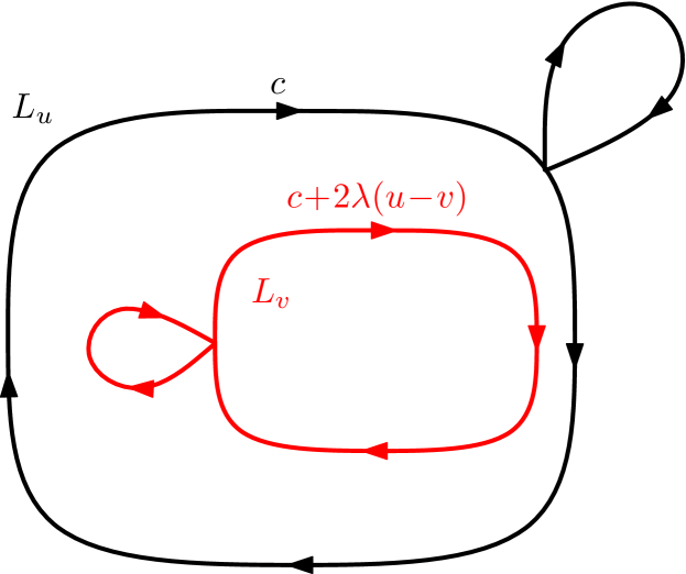
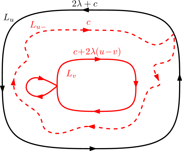
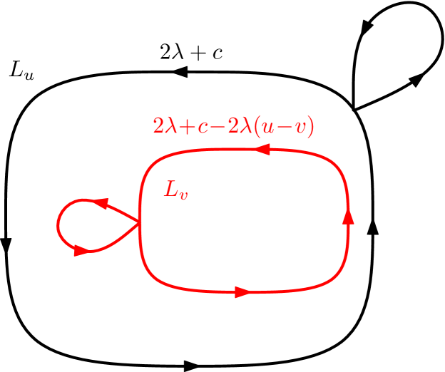
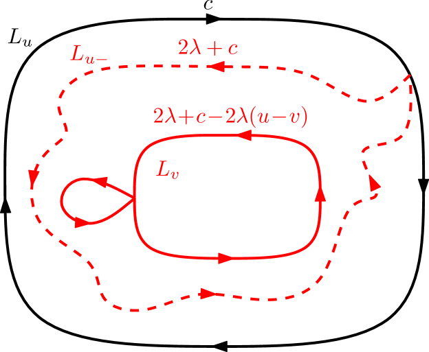
Given a transient càdlàg sequence of adjacent quasisimple loops , we use the term continuum level loop boundary conditions to describe the boundary values given by the following rule. Assume that the loop has boundary value to the left-side and to the right-side, and assume that for some . Then, for , the boundary value of is
See Figure 1.2.2. Note that, once we know the boundary value of a loop in the sequence, we can tell the boundary values of all loops , for , by the continuum level loop boundary conditions.
Suppose that is a domain with harmonically non-trivial boundary. We call a sequence of quasisimple loops in a transient càdlàg sequence of adjacent quasisimple loops disconnecting from if the sequence satisfies the following properties.
-
(1)
There exists a sequence of reals such that
and that, for all , the loops have the same orientation for which is different from the orientation of .
-
(2)
For each , the loop disconnects from .
-
(3)
For , the loop is contained in the closure of the connected component of that contains . Moreover, the sequence is càdlàg under Carathéodory topology seen from , and for each , the loop has nonempty intersection with its left limit.
-
(4)
The sequence is transient: the loop converges to in Hausdorff metric as .
The continuum level loop boundary conditions for a transient càdlàg sequence of quasisimple loops in can be defined similarly.
The following two theorems explains that the continuum exploration process of starting from an interior point is a càdlàg sequence of quasisimple loops.
Theorem 1.2.1.
Fix a connected domain with harmonically non-trivial boundary and a starting point . Suppose that is a on with some boundary values and that is a transient càdlàg sequence of adjacent quasisimple loops in disconnecting from . There exists a coupling between and such that the following domain Markov property is true. For any stopping time , the conditional law of given is a on whose boundary value agrees with the boundary value of on and is given by the continuum level loop boundary conditions on .
Suppose that is a whole-plane modulo a global additive constant in and that is a random transient càdlàg sequence of adjacent quasisimple loops disconnecting the origin from infinity. There is a coupling between and such that the following domain Markov property is true. For any stopping time , the conditional law of given is a (modulo a global additive constant in ) on whose boundary value is given by the continuum level loop boundary conditions on .
Theorem 1.2.2.
In the coupling of a and a random sequence of quasisimple loops as in Theorem 1.2.1, the sequence is almost surely determined by the field viewed as a distribution modulo a global additive constant in .
In the coupling between a whole-plane and a random sequence of quasisimple loops given by Theorem 1.2.1, we call the sequence the alternating continuum exploration process of starting from the origin targeted at ; and we call the sequence of transition times.
The following two theorems explain the interaction behavior between two alternating continuum exploration processes.
Theorem 1.2.3.
Suppose that is a whole-plane modulo a global additive constant in . Fix two starting points . For , let be the alternating continuum exploration process of starting from targeted at . Define
Then, almost surely, the loops and coincide; moreover, the two sequences of loops and coincide.
Theorem 1.2.4.
Suppose that is a whole-plane modulo a global additive constant in . Fix three points . For , let be the alternating continuum exploration process of starting from targeted at ; and denote by the connected component of that contains . Then there exists a number such that
Given , the two sequences continue towards their target points respectively in a conditionally independent way.
The following theorem explains that all the alternating continuum exploration processes of give a tree-structure of the plane.
Theorem 1.2.5.
Suppose that is a whole-plane modulo a global additive constant in . Suppose that is any countable dense set and, for each , let be the alternating continuum exploration process of starting from targeted at . Then the collection almost surely determines the field and its law does not depend on the choice of . Moreover, the collection forms a tree structure in the sense that, almost surely, any two sequences of quasisimple loops merge eventually.
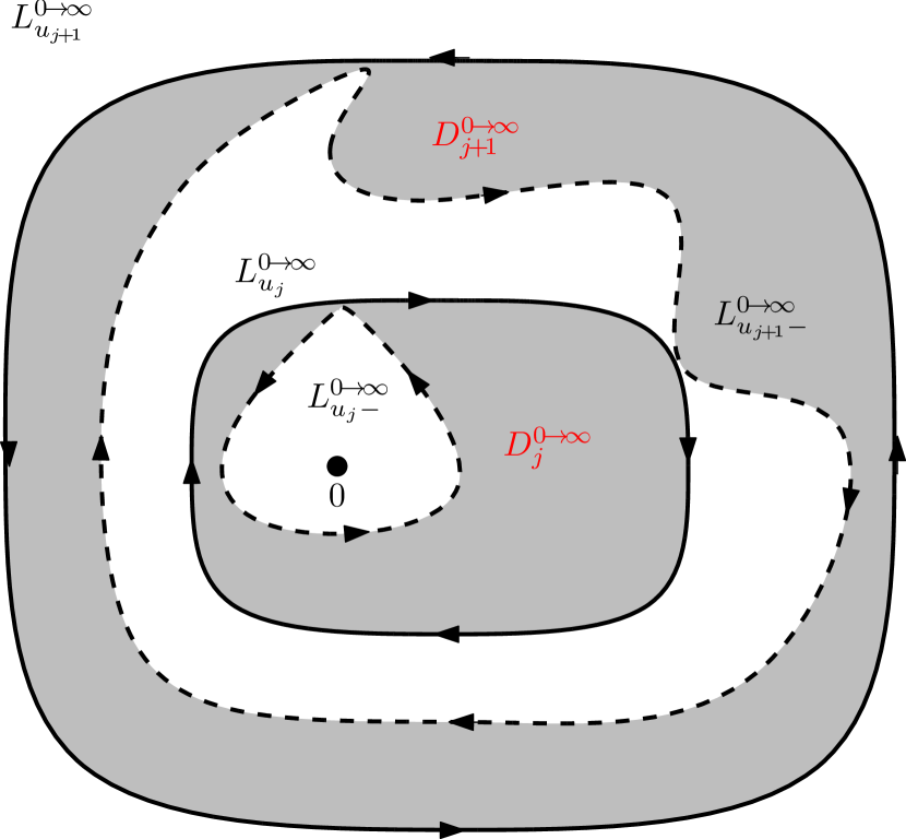
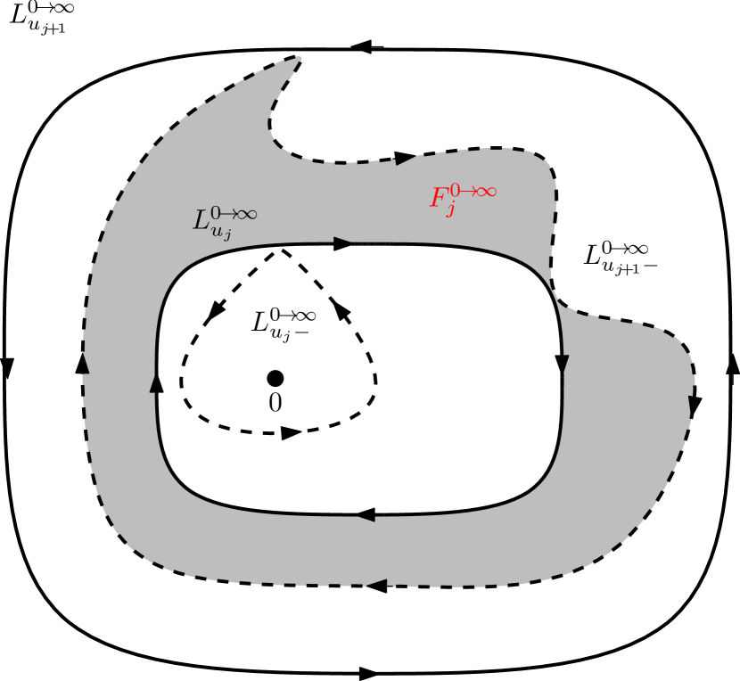
Next, we will explain the “reversibility” of the alternating continuum exploration processes. Suppose that is a whole-plane modulo a global additive constant in . Let be the alternating continuum exploration process of starting from the origin targeted at where is the sequence of transition times. For each transition time , define the corresponding transition region by
In other words, the region is the domain lying between the loops and . See Figure 1.2.3(a). We call the sequence of transition regions of starting from the origin targeted at . For each transition time , define the corresponding stationary region by
In other words, the region is the domain lying between and . See Figure 1.2.3(b). We call the sequence of stationary regions of starting from the origin targeted at .
Theorem 1.2.6.
Suppose that is a whole-plane modulo a global additive constant in . Let (resp. ) be the sequence of transition regions (resp. the sequence of stationary regions) of starting from the origin targeted at . Let (resp. ) be the sequence of transition regions (resp. the sequence of stationary regions) of starting from targeted at the origin. Then, almost surely, the two unions
coincide; moreover, the two unions
coincide.
1.3 Relation to previous works and outline
We prove Theorems 1.2.1 to 1.2.6 in Section 3. Following is the outline of Section 3.
- •
-
•
In Section 3.2, we explain how to get the continuum exploration process of from discrete exploration process of .
- •
- •
- •
Acknowledgements. The current project is motivated by [MS13], and we appreciate Jason Miller and Scott Sheffield for helpful discussions on both [MS13] and the current paper. We also thank Richard Kenyon, Samuel Watson, and Wendelin Werner for helpful discussions. H. Wu’s work is funded by NSF DMS-1406411.
2 Sequence of level loops starting from interior
2.1 The whole-plane
In this section, we will give an overview of whole-plane , we refer the proofs related to the properties of whole-plane to [MS13, Section 2.2]. For the construction and the properties of ordinary , one can consult [MS16a, Section 3] or [WW16, Section 2.2].
For a domain , we denote by the space of functions with compact support in and denote by the space of those with . We denote by the inner product. Let denote the Hilbert space closure of equipped with the Dirichlet inner product. Let be a sequence of i.i.d. one-dimensional standard Gaussian (with mean zero and variance one). Let be an orthonormal basis of . The whole-plane modulo a global additive constant in is an equivalence class of distributions (where two distributions are equivalent when their difference is a constant in ), a representative of which is given by . For each , the limit almost surely exists, thus we write
We think of as being defined up to an additive constant in because
We can fix the additive constant by setting for some fixed with .
Fix and with . The whole-plane modulo a global additive constant in is an equivalence class of distributions (where two distributions are equivalent when their difference is a constant in ). An instance can be generated by
-
(1)
sampling a whole-plane modulo a global additive constant in , and then
-
(2)
choosing independently a uniform random variable and fixing a global additive constant for by requiring that .
Suppose that is a zero-boundary on a proper domain with harmonically non-trivial boundary. We can consider modulo a global additive constant in by restricting to functions in . Fix with . We can also consider modulo a global additive constant in by replacing by where is chosen so that .
The following proposition describes the domain Markov property of whole-plane .
Proposition 2.1.1.
Suppose that is a whole-plane modulo a global additive constant in (resp. in ) and that is open and bounded. The conditional law of given is that of a zero-boundary on plus the harmonic extension of its boundary values from to which is defined modulo a global additive constant in (resp. in ).
Proof.
[MS13, Proposition 2.8]. ∎
The following proposition explains that infinite volume limits of ordinary converge to the whole-plane .
Proposition 2.1.2.
Suppose that is any sequence of domains with harmonically non-trivial boundary containing the origin such that as . For each , let be an instance of on with boundary conditions which are uniformly bounded in . Fix , we have the following.
-
(1)
As , the laws of restricted to , viewed as a distribution modulo a global additive constant in , converge in total variation to the law of whole-plane restricted to modulo a global additive constant in .
-
(2)
Fix with which is constant and positive on . As , the laws of restricted to , viewed as a distribution modulo a global additive constant in , converge in total variation to the law of whole-plane restricted to modulo a global additive constant in .
Proof.
[MS13, Proposition 2.10]. ∎
Proposition 2.1.3.
Suppose that with harmonically non-trivial boundary and is a on with some boundary data. Fix open and bounded with . The law of modulo a global additive constant in (resp. in ) is mutually absolutely continuous with respect to the law of whole-plane restricted to modulo a global additive constant in (resp. in ).
Proof.
[MS13, Proposition 2.11]. ∎
The notion of local set, first introduced in [SS13] for ordinary , serves to generalize the domain Markov property to random subsets. There is an analogous theory of local sets for the whole-plane .
Suppose that is a whole-plane modulo a global additive constant in (resp. in ) and suppose that is a random closed subset which is coupled with such that has harmonically non-trivial boundary. We say that is a local set of if there exists a law on pairs , where is a distribution with the property that is almost surely a harmonic function, such that a sample with the law can be produced by
-
(1)
choosing the pair ,
-
(2)
sampling an instance of zero-boundary on and setting ,
-
(3)
considering the equivalence class of distribution modulo a global additive constant in (resp. in ) represented by .
The definition is equivalent if we consider as being defined modulo a global additive constant in (resp. in ). We write for the function described above. We say that is the conditional mean of given and .
By this definition, Theorem 1.1.1 implies that, for any stopping time , the sequence of loops is a local set for the whole-plane modulo a global additive constant in .
The following propositions are properties of local sets of whole-plane .
Proposition 2.1.4.
Suppose that is a whole-plane modulo a global additive constant in or in . Suppose that are random closed subsets and that and are couplings for which are local. Let denote the random closed subset which is given by first sampling , then sampling conditionally independent given , and then taking the union of and . Then is also local for .
Proof.
[MS13, Proposition 2.14]. ∎
Proposition 2.1.5.
Let be connected local sets of whole-plane which are conditionally independent and . Then is almost surely a harmonic function in that tends to zero along all sequences of points in that tend to a limit in a connected component of (which consists of more than a single point) or that tend to a limit on a connected component of (which consists of more than a single point) at a point that is a positive distance from either or .
Proof.
[MS13, Proposition 2.15]. ∎
Proposition 2.1.6.
Suppose that is a local set for a whole-plane modulo a global additive constant in (resp. in ). Fix open and bounded and assume that almost surely. Let be a domain with harmonically non-trivial boundary such that with and let be a on .
-
(1)
There exists a law on random closed set which is mutually absolutely continuous with respect to the law of such that is a local set for .
-
(2)
Let be the function which is harmonic in and which has the same boundary behavior as on . Then the law of , modulo a global additive constant in (resp. in ), and the law of are mutually absolutely continuous.
-
(3)
If is almost surely determined by , then is almost surely determined by .
Proof.
[MS13, Proposition 2.16]. ∎
2.2 Alternating height-varying sequence of level loops
In [WW16, Sections 2, 3.3, 3.4], we studied the level line of starting from a boundary point targeted at a boundary point or an interior point. We briefly recall some basic properties.
Suppose that is a on whose boundary value is piecewise constant and changes only finitely many times. Fix a starting point and a target point . The level line of starting from targeted at is a random curve coupled with such that the following is true. Suppose that is any stopping time. Then, given , the conditional law of restricted to is the same as s in each connected component whose boundary value is consistent with on and is to the right of and is to the left of . In this coupling, the curve is almost surely determined by and is almost surely continuous up to and including the continuation threshold. Generally, for , the level line of with height is the level line of .
In particular, suppose that is a zero-boundary on , let be the level line of starting from targeted at with height . We parameterize the curve by minus the log of the conformal radius of seen from :
Then the law of is the same as radial process starting with with two force points next to the starting point and the corresponding weights are given by [WW16, Proposition 3.3.1]
Suppose that is the corresponding radial Loewner evolution. The continuation threshold of is hit at the following time
which is almost surely finite. Let be the connected component of that contains , and let be the oriented boundary of . We know that is independent of the choice of . We call the level loop of with height starting from targeted at . The loop is almost surely determined by and
We recall several results from [WW16] that we will use later in the current paper.
Lemma 2.2.1.
Suppose that is a on with piecewise constant boundary data which changes a finite number of times. Let be the level line of with height starting from targeted at .
-
(1)
Suppose that has boundary value to the right of and to the left of . To have non-trivial (i.e. has strictly positive length), we must have
-
(2)
Suppose that has boundary value to the right of and to the left of . Then the probability of to reach is zero if one of the following two conditions holds.
-
•
and ;
-
•
and .
-
•
-
(3)
Suppose that has boundary value on some open interval which does neither contain nor . If hits with strictly positive probability, then .
Proof.
[WW16, Remark 2.5.15]. ∎
Lemma 2.2.2.
Suppose that is a on whose boundary value is piecewise constant, changes only finitely many times. For each and , let be the level line of with height starting from targeted at infinity. Fix .
-
(1)
If , then almost surely stays to the left of .
-
(2)
If , then may intersect and, upon intersecting, the two curves merge and never separate.
Proof.
[WW16, Theorem 1.1.4]. ∎
Lemma 2.2.3.
Suppose that is a zero-boundary on . Fix a height and a target point . Let be the level loop of starting from the boundary targeted at . Then we have the following.
-
(1)
is oriented either clockwise or counterclockwise and is homeomorphic to the unit disc.
-
(2)
.
-
(3)
Given , the conditional law of restricted to each connected component of is the same as ’s whose boundary value is zero on , is to the right of , and is to the left of .
Moreover, the loop is almost surely determined by ; and any oriented loop in that satisfies the above three properties almost surely coincides with .
Proof.
[WW16, Lemmas 3.3.5 and 3.3.6]. ∎
Suppose that is a zero-boundary on . Fix and a target point . We will introduce the upward height-varying sequence of level loops. Set
Let be the level loop of with height . Then, given , the conditional mean of restricted to is
Moreover,
If is clockwise, we stop and set ; if not, we continue. Generally, given and is counterclockwise, let be the level loop of restricted to with height . If is clockwise, we stop and set ; if not, we continue. At each step, we have chance to stop; thus we will stop at some finite time which we call transition step. We call the sequence upward height-varying sequence of level loops with height difference starting from targeted at . We summarize some basic properties of this sequence in the following.
-
(a)
The transition step satisfies the geometric distribution
-
(b)
For , the loop is counterclockwise; the loop is clockwise.
-
(c)
For , let be the conditional mean of restricted to given , we have
Symmetrically, we could define downward height-varying sequence of level loops of . For the downward height-varying sequence , the transition step satisfies the geometric distribution. The loops are clockwise and the loop is counterclockwise. Let be the conditional mean of restricted to given , we have
Next, we will introduce alternating height-varying sequence of level loops. Suppose that is a zero-boundary on . Fix and a target point . Assume that is oriented counterclockwise. We start by the upward height-varying sequence of level loops of . Let be the transition step and denote sequence by . Let be the conditional mean of restricted to given , then
We continue the sequence by the downward height-varying sequence of level loops of restricted to . Let be the its transition step and denote the sequence by . Let be the conditional mean of restricted to given , then
Set .
Generally, given for some , we have
We continue the sequence by the upward height-varying sequence where is its transition step. We then continue the sequence by the downward height-varying sequence where is its transition step. Set
and let be the conditional mean of restricted to given , we have
In this way, we obtain an infinite sequence which we call alternating height-varying sequence of level loops of with height difference starting from (counterclockwise) targeted at .
If we orient clockwise, we can define alternating height-varying sequence similarly, the only difference is that we start by downward height-varying sequence.
Proposition 2.2.4.
The alternating height-varying sequence of level loops of is almost surely determined by the field.
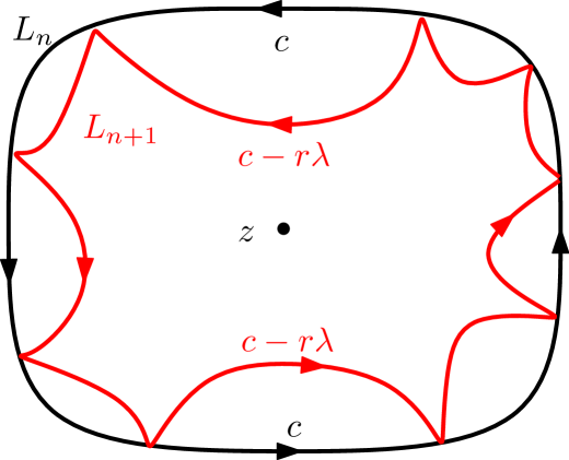
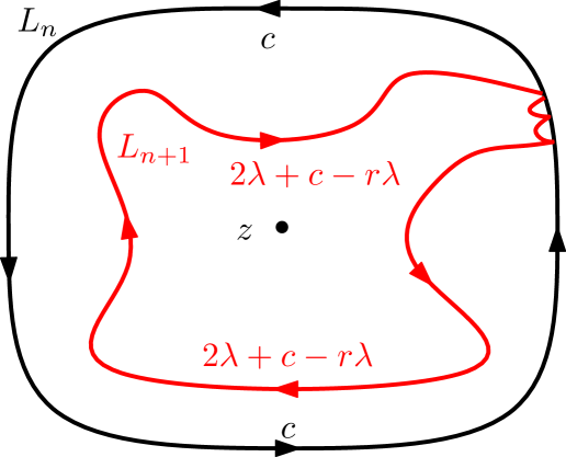
Note that, in the alternating height-varying sequence of level loops with height difference , each loop has the height of the form
The relation between the heights of two neighbor loops is explained in Figure 2.2.1.
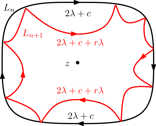
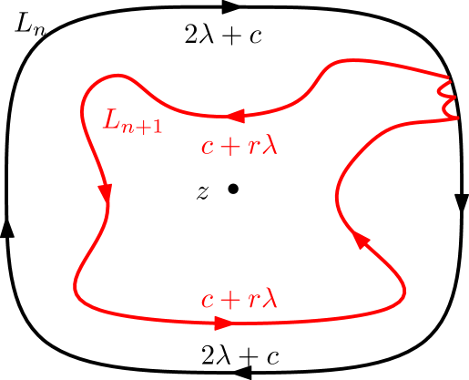
From the construction, we know that the alternating height-varying sequence satisfies the following domain Markov property.
Proposition 2.2.5.
Suppose that is an alternating height-varying sequence of level loops. For any stopping time , given , let be the conformal map from onto such that , then the conditional law of the sequence is the same as alternating height-varying sequence of level loops.
Proposition 2.2.6.
The alternating height-varying sequence of level loops starting from targeted at is transient: the loop converges to in Hausdorff metric as .
Proof.
We may assume that the target point is the origin and that is counterclockwise. Suppose that the height difference is for .
First, we show that there exist constants , and such that
Set . Let be the first transition step of the sequence . On the event , the level loop is of height , thus (by Lemma 2.2.1). Therefore,
Thus, there exists such that
Next, we show the transience. For , let be the conformal map from onto such that . From the domain Markov property of the sequence , we know that is an i.i.d. sequence. By the first step, we have
By Borel-Cantelli Lemma, almost surely, there exists a sequence such that
In particular,
Denote by . We only need to show that the sequence is transient. We will show by induction on .
For , on the one hand, we have ; on the other hand, since for all , we have . Combining these two facts, we have that .
Assume that the claim holds for , let us consider . We know that , it is then sufficient to argue that . Note that is the conformal map from onto with . Let . Since , the set is still contained in . Let be the conformal map from onto with . Then . Since for all , we have . Thus
This completes the proof. ∎
The following proposition describes the target-independence of the sequence of level loops.
Proposition 2.2.7.
Fix . Suppose that is a zero-boundary on . Fix two points . For , let be the alternating height-varying sequence of level loops of with height difference starting from targeted at ; and denote by the connected component of that contains . Then there exists a number such that
Given , the two sequences continue towards their target points respectively in a conditionally independent way.
Proof.
[WW16, Section 3.5]. ∎
Suppose that is an alternating height-varying sequence of level loops starting from targeted at . We want to change the index of the loops so that they are indexed by minus the log of the conformal radius seen from . Namely, we construct the sequence so that
We call the obtained sequence alternating height-varying sequence of level loops indexed by minus the log conformal radius seen from .
Next, we will introduce a whole-plane version of alternating height-varying sequence of level loops. Before this, we briefly recall the conformal radius seen from infinity. When is a simply connected compact set, its complement is a simply connected domain in the Riemann sphere that contains . Let be the unique bijective conformal map with and the expansion at of the following form
We call the derivative of at , denoted by ; call the conformal radius of seen from , denoted by . Note that, for ,
For each , let be a on with zero-boundary value. The boundary is oriented either clockwise or counterclockwise. We can uniquely generate the alternating height-varying sequence of level loops of starting from targeted at : , where the loops are indexed by minus log conformal radius seen from . Namely,
For each , let be the conformal map from onto with . The following lemma explains that the family is convergent.
Lemma 2.2.8.
The family of conformal maps converges weakly to some limit with respect to the topology of local uniform convergence. Namely, for every and every compact interval , the map converges weakly to uniformly on where is the loop such that is the conformal map from onto with .
Proof.
We will show that there exist universal finite constants such that the following is true. For any small, there exists a coupling between and such that
This will imply the conclusion.
For any small, consider the sequence . By the first step in the proof of Proposition 2.2.6, we know that there exist universal constants so that the probability of the event is bounded uniformly from below. Therefore, given , we can couple and so that the probability of the event is bounded uniformly from below.
By the domain Markov property in Proposition 2.2.5 and the scaling invariance, there exists a coupling between and so that
where is some finite universal constant. On the event , we couple the processes to be identical for . This completes the proof. ∎
Suppose that is the limit family of conformal maps in Lemma 2.2.8 and that is the corresponding sequence of loops, i.e. is the conformal map from onto with . Note that the loops in the sequence are indexed by minus the log of conformal radius seen from :
We also say that the alternating height-varying sequence of level loops converges weakly to with respect to the topology of local uniform convergence. Clearly, the sequence is a transient sequence of adjacent simple loops disconnecting the origin from infinity by Proposition 2.2.6. We now are ready to complete the proof of Theorem 1.1.1.
Proof of Theorem 1.1.1.
First, we construct a coupling between whole-plane and a transient sequence of adjacent simple loops. For each , let be a on with zero-boundary value. Let be the alternating height-varying sequence of level loops of starting from targeted at indexed by minus the log conformal radius seen from . Let be the corresponding sequence of conformal maps: is the conformal map from onto with . On the one hand, from Lemma 2.2.8, we know that the sequence converges weakly to and the sequence converges weakly to with respect to the topology of local uniform convergence. On the other hand, the s , viewed as distributions defined modulo a global additive constant in , converge to a whole-plane , modulo a global additive constant in , as by Proposition 2.1.2. This gives a coupling of a whole-plane and a transient sequence of adjacent simple loops disconnecting the origin from .
Second, we show that the coupling satisfies the desired domain Markov property. For each and , given , the conditional law of restricted to is the same as a with boundary value
modulo a global additive constant in ; and the conditional law of restricted to other connected components of is the same as s with boundary value given by level loop boundary conditions with height difference . The convergence of to implies that, given , the conditional law of restricted to is the same as s with boundary values given by level loop boundary conditions with height difference . This implies that the coupling satisfies the desired domain Markov property at deterministic times .
For general stopping time , suppose that is deterministic and . The conditional law of given is the same as in . Let be the alternating height-varying sequence of level loops of restricted to starting from targeted at .
-
(a)
By Proposition 2.2.4, we know that the sequence coincides with the sequence almost surely.
-
(b)
By Proposition 2.2.5, we know that the sequence satisfies the desired domain Markov property for any stopping time.
Combining these two facts, the coupling satisfies the desired domain Markov property for the stopping time . Since is arbitrary, the domain Markov property holds for any stopping time .
Finally, we prove the conclusion for general domain . Since the law of (modulo a global additive constant in ) in a small neighborhood of the origin changes in an absolutely continuous way when we replace with . We can couple the sequence of loops with the field as if the domain were up until the first time that the sequence of the loops exits the small neighborhood. Then the usual boundary emanating level lines allow us to extend the sequence of level loops uniquely by Proposition 2.1.6. ∎
In the coupling as in Theorem 1.1.1, we call the sequence the alternating height-varying sequence of level loops starting from the origin targeted at infinity (resp. starting from targeted at ) of with height difference when (resp. when ).
2.3 Interaction
In this section, we will discuss the interaction behavoirs.
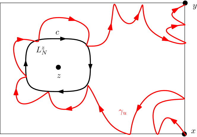
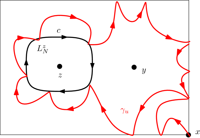
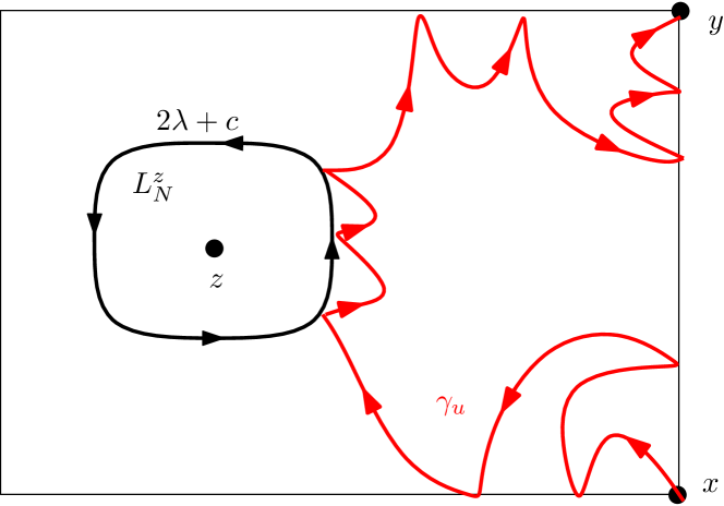
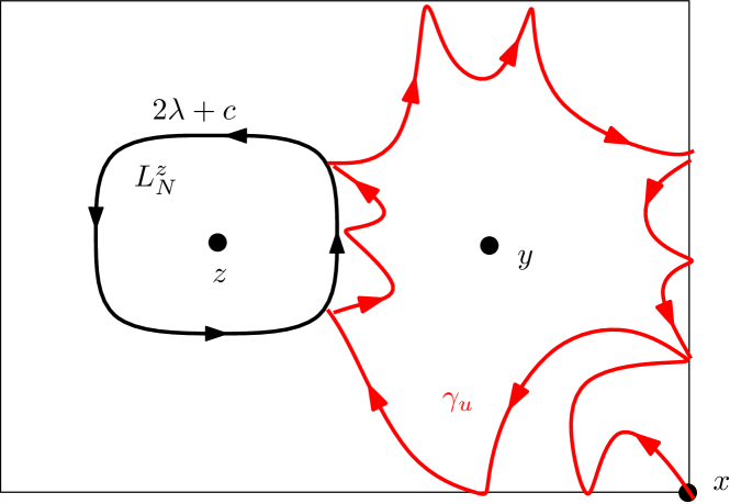
Proposition 2.3.1.
Fix and a domain with harmonically non-trivial boundary. Fix three points and . Let be a on , let be the alternating height-varying sequence of level loops of with height difference starting from targeted at , and let be the level line of with height starting from targeted at . For any -stopping time , assume that the loop does not hit and has boundary value to the left-side and to the right-side. On the event , we have that
Moreover, the level line stays outside of . See Figure 2.3.1.
Proof.
We may assume that is clockwise, and the case that is counterclockwise can be proved similarly.
First, we show that . Given , denote by the field of restricted to . We know that the conditional law of is the same as with boundary value on . Moreover, the curve is also the level line of with height . By Lemma 2.2.1 Item (3), we have that .
Next, we show that stays outside of . We prove by contradiction. Assume that has non-trivial pieces in . Given , the conditional law of , restricted to the connected components of that are in , is the same as whose boundary values are along . For these s, to have non-trivial level lines with height starting from , we must have which contradicts with the fact that . ∎
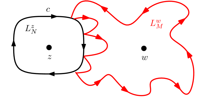
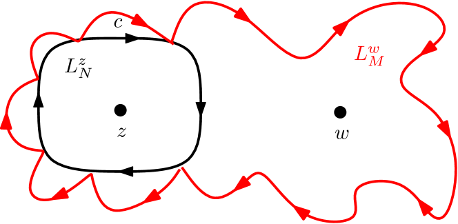
Proposition 2.3.2.
Fix . Let be a whole-plane modulo a global additive constant in . Fix two starting points . Let (resp. ) be the alternating height-varying sequence of level loops of with height difference starting from (resp. starting from ) targeted at . Let be any -stopping time such that does not disconnect from . Assume that has boundary value to the left-side and to the right-side. Let be any stopping time with respect to the filtration
Suppose that hits and has height . Then
Moreover, the loop stays outside of . See Figure 2.3.2.
Proof.
We may assume that is clockwise, and the case that is counterclockwise can be proved similarly.
First, we show that . Given , denote by the field of restricted to . We have the following observations.
-
(a)
Given , the conditional law of is the same as on with boundary value .
-
(b)
Given , the sequence is coupled with in the same way as in Theorem 1.1.1 for , up to the first time that the loop exits .
When hits , the pieces of contained in are level lines of with height . By Lemma 2.2.1 Item (3), we have that .
Next, we show that stays outside of . This can be proved similarly as in the proof of Proposition 2.3.1. ∎
Proposition 2.3.3.
Fix . Let be a whole-plane modulo a global additive constant in . Fix two starting points . Let (resp. ) be the alternating height-varying sequence of level loops of with height difference starting from (resp. starting from ) targeted at . Define the stopping times
Then, almost surely, the loop coincides with .
The proof of Proposition 2.3.3 needs the following lemma.
Lemma 2.3.4.
Assume the same notations as in Proposition 2.3.3. Let be the connected component of that contains . Let be any stopping time with respect to the following filtration
On the event
we have almost surely that the loop is contained in the closure of .

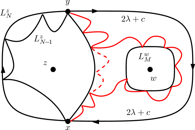
Proof.
We may assume that is clockwise, and the case that is counterclockwise can be proved similarly. We have the following observations.
-
(a)
Given , the conditional law of restricted to is the same as with boundary value which is some multiple of .
-
(b)
Note that has two special points and so that the clockwise part of from to is part of and the counterclockwise part of from to is part of . See Figure 2.3.3(a). Given , the conditional law of restricted to is the same as with boundary value on and
-
(c)
Given , the sequence is coupled with restricted to in the same way as in Theorem 1.1.1 for , up to the first time that the loop exits .
-
(d)
Given and on the event , the conditional law of restricted to is the same as with certain boundary data which is on .
Assume that the loop has height and we will prove the conclusion by contradiction. Assume that enters . Then the pieces of that are contained in are level lines of restricted to with height , thus by Lemma 2.2.1 Item (1). Since is a multiple of and is also a multiple of , we have that .
First, we show that the loop can only exit through or . Combining with Lemma 2.2.1 Item (3), we have that the loop can not hit the interior of from inside. We only need to explain that can not exit through the interior points of .
Assume that the loop does exit through an interior point of and assume that the boundary value of the field along is to the inside of and is to the outside of .
-
(a)
Since the loop hits interior points of , we have by Lemma 2.2.1 Item (3).
-
(b)
Since the pieces of outside of are level lines with height , we have by Lemma 2.2.1 Item (1).
Combining these two facts with , we get a contradiction.
Since is a loop, if it exits , it has to come back to . With a similar analysis as above, we know that can only come back to through or . Therefore, if exits , it has to exit through one of and come back to through the other one.
Second, we show that has to be clockwise. If the loop is counterclockwise, then the boundary value of restricted to is on . Since , the level lines of , restricted to , with height can not hit by Lemma 2.2.1 Item (2), and the field of , restricted to , can not have non-trivial level line with height starting from . This contracts that exits or comes back to through .
Finally, we show that there exists a level loop of restricted to with height that is contained in . Denote by the field of restricted to . Since is clockwise, the field has boundary value along . Since the loop has height and exits at or , we have by Lemma 2.2.1 Item (2). Therefore, we have .
Consider the level lines of with height starting from some points on . Since , these level lines can be continued towards both and after they hit by [WW16, Lemma 2.3.1]. This implies that there exists a complete level loop of with height contained in the closure of and touching . We denote it by . See Figure 2.3.3(b).
Now, we have the following observations.
-
(a)
The loop is a level loop of restricted to with height starting from targeted at .
-
(b)
The loop is a level loop of restricted to with height starting from targeted at .
Combining these two facts with Lemma 2.2.3, we get a contradiction. ∎
Proof of Proposition 2.3.3.
We may assume that is clockwise and it has the boundary value to the left-side where is a multiple of .
First, we show that coincides with for some . Let be the first loop in that hits the inside of . By Lemma 2.3.4, we know that is contained in the closure of . Suppose that the loop has height . Since hits the inside of , we have by Lemma 2.2.1 Item (3). Note that is a multiple of and is also a multiple of , thus for some integer . In particular, the loop has height .
If is clockwise, then has to coincides with , since both of and are level loops of , restricted to , with height starting from targeted at (Lemma 2.2.3).
If is counterclockwise, we have the following observations.
-
(a)
The loop is a level loop of restricted to with height starting from targeted at .
-
(b)
The sequence is the alternating height-varying sequence of restricted to with height difference starting from targeted at . Thus the sequence starts by downward height-varying sequence, changes the orientation after some finite step, and continues with upward height-varying sequence etc.
Combining these two facts, we know that coincides with for some integer .
Next, we show that coincides with . By the first step, we know that coincides with for some . Since disconnects from , we have . Symmetrically, the loop coincides with for some . Combining these two facts, we have that coincides with . ∎
Proof of Theorem 1.1.3.
Suppose that, for , the sequence is the alternating height-varying sequence of level loops of with height difference starting from targeted at indexed by minus the log of the conformal radius seen from , and define
By Proposition 2.3.3, there exists some finite such that ; we define to be the inf of such times. We have the following observations.
-
(a)
For any , we have ; whereas, , thus .Therefore .
-
(b)
By Proposition 2.3.3, we have , thus .
Combining these two facts, we have that almost surely. By symmetry, we have almost surely.
We have the following observations.
-
(a)
The sequence is the alternating height-varying sequence of level loops of restricted to .
-
(b)
The sequence is the alternating height-varying sequence of level loops of restricted to .
-
(c)
The loops and coincide.
Combining these three facts and Proposition 2.2.4, we have that
This completes the proof. ∎
Proof of Theorem 1.1.2.
We only need to show the conclusion for , and the proof for follows from absolute continuity.
Suppose that is a whole-plane modulo a global additive constant in . Suppose that and are two alternating height-varying sequences of level loops of starting from the origin targeted at indexed by minus the log of the conformal radius seen from , and they are coupled with so that, given , they are conditionally independent.
Pick any and let be the alternating height-varying sequence of level loops of starting from targeted at . By Theorem 1.1.3, for , there exists a finite number such that
Therefore, there exists a finite number such that
Let be the inf of such times. The scaling invariance of the coupling implies that the law of is scaling invariant. Thus almost surely. Therefore, almost surely,
∎
Proof of Theorem 1.1.4.
Consider , let be any stopping time such that both and are contained in . Given , denote by the field of restricted to . For , let be the alternating height-varying sequence of level loops of with height difference starting from targeted at ; and denote by the connected component of that contains . We have the following observations.
-
(a)
From the target-independence in Proposition 2.2.7, we know that there exists a number such that
Given , the two sequences continue towards their target points respectively in a conditionally independent way.
-
(b)
By Theorem 1.1.2, for , we know that the collection of the loops in the union of and is the same as the collection of the loops in the sequence .
Combining these two facts, we obtain the conclusion. ∎
Proof of Theorem 1.1.5.
For , let be the -algebra generated by . Fix and define for .
First, we argue that, to obtain the conclusion, it is sufficient to show that
| (2.3.1) |
We have the following observations.
-
(a)
Since is integrable, the martingale converges to almost surely and in .
-
(b)
Assuming Equation (2.3.1) holds, we have that converges to in .
Combining these two facts, we have that almost surely, which implies the conclusion.
Next, we show Equation (2.3.1). For each , let be the Green’s function of . Since has Lebesgue measure zero, we can view as a function defined on and the value of on will not affect later integrations. Note that has countably many connected components. If and are contained in the same connected component of , then is exactly the Green’s function of that component taking value at ; if and are contained in distinct components of , then . Since the sequence is decreasing, the sequence is non-increasing for fixed and .
Let be a compact set which contains the support of . Then
Note that is bounded by which is integrable; and that , for fixed and , since and will be disconnected by for large enough. Thus , which implies Equation (2.3.1). ∎
3 Continuum exploration process starting from interior
3.1 Growing process of
In this section, we will introduce a continuum growing process of . We first recall some features of and refer to [SW12] for details and proofs; and then recall the construction and properties of the continuum growing process of and refer to [WW13] for details and proofs.
is a random collection of non-nested disjoint simple loops that possesses Conformal Invariance and Domain Markov Property. The loops in are -type loops for some ; moreover, for each such value of , there exists exactly one distribution that has -type loops. We denote the corresponding by for . Throughout the current paper, we fix .
We call a bubble in if is a simple loop and contains exactly one point; we call the point in the root of , denoted by . Consider a in , draw a small disc with center and radius , and let be the loop in that intersects with largest radius. Define the quantity . The law of normalized by converges to a limit measure (see [SW12, Section 4]), denoted by . Define -bubble measure by
where is Lebesgue measure on . When , the bubble measure is conformal invariant. Namely, for any Möbius transformation of , we have (see [WW13, Lemma 6]).
Let be a Poisson point process with intensity . (In other words, let be a Poisson point process with intensity , and then arrange the bubbles according to time , i.e. denote the bubble by if , and is empty set if there is no that equals .) Clearly, there are only countably many bubbles in that are not empty set.
We will construct a growing process from the sequence of bubbles . Define to be the first time that surrounds the origin. Consider the sequence . For each , the bubble does not surround the origin. Define to be the conformal map from the connected component of that contains the origin onto the unit disc such that and . We have the following properties. See [SW12, Section 7]
-
(a)
The stopping time has exponential law: .
-
(b)
For small, let be the times before at which the bubble has radius greater than . Define . Then almost surely converges to some conformal map in Carathéodory topology seen from the origin as goes to zero. Therefore, can be interpreted as , and maps some simply connected open subset of onto .
-
(c)
Define . Then has the same law as the loop in that surrounds the origin. In particular, is a simple loop. We give the clockwise orientation to the loop .
-
(d)
Generally, for each , we can define , and maps some simply connected open subset of onto . We denote by the boundary of which is a quasisimple loop. We give the counterclockwise orientation to . Note that is the conformal map from the connected component of that contains the origin onto with and .
-
(e)
For each , let be the boundary of . See Figure 3.1.1. Then is a quasisimple loop and we give counterclockwise orientation to it.
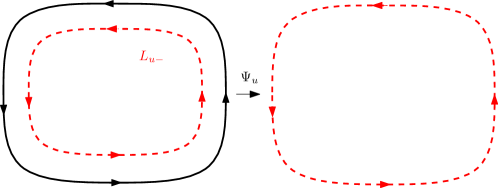
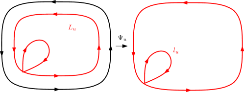
From the above construction, we get a sequence of quasisimple loops from the sequence of bubbles . We will show the sequence is càdlàg. Before this, we need to be precise about the topology. Fix and consider a sequence of quasisimple loops . For each , denote by the connected component of that contains . We say that the sequence converges to a quasisimple loop in Carathéodory topology seen from if the sequence converges to in Carathéodory topology seen from where is the connected component of that contains .
Lemma 3.1.1.
Consider the sequence of quasisimple loops .
-
•
For each , the right limit exists and equals almost surely ;
-
•
For each , the left limit exists and equals almost surely.
Proof.
First, we show the conclusion for the right limit. For and , we have the following observations.
-
(a)
The map (resp. ) is the conformal map from the connected component of (resp. ) that contains the origin onto with and (resp. and ).
-
(b)
As , the map converges almost surely to in Carathéodory topology seen from the origin.
Combining these two facts, we have that the right limit exists and equals .
Next, we show the conclusion for the left limit. For and , we have the following observations.
-
(a)
The map (resp. ) is the conformal map from the connected component of (resp. ) that contains the origin onto with and (resp. and ).
-
(b)
As , the map converges almost surely to in Carathéodory topology seen from the origin.
Combining these two facts, we have that the left limit exists and equals . ∎
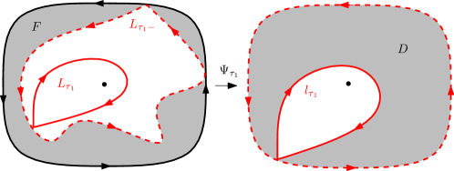
Consider the Poisson point process and keep the same notations as above. Recall that is the composition of maps which is the conformal map from the connected component of that contains the origin onto with and . The loop is the boundary of . In other words, is the conformal map from the connected component of that contains the origin, denoted by , onto with and .
Define the compact set to be the domain lying between and (see Figure 3.1.2):
and denote its law by . Note that the complement of in the Riemann sphere has two connected components: and .
The bubble is the first bubble in that surrounds the origin. Define the compact set to be the domain lying between and (see Figure 3.1.2):
and denote its law by . Note that the complement of in the Riemann sphere has two connected components: and ; and that the interior of is simply connected.
The loop has the same law as the loop in in the unit disc that surrounds the origin. Define to be the annulus lying between and :
and denote its law by .
From the above analysis, we have the following relation between the pair and the loop in .
Lemma 3.1.2.
Suppose that is a pair of compact sets sampled according to the law . Let be the conformal map from the connected component of that contains the origin onto with and . Then the law of the compact set is the same as the law of the closure of an annulus with law .
3.2 From discrete to continuum exploration of
In this section, we will explain how to couple with the sequence of quasisimple loops introduced in Section 3.1. Roughly speaking, the sequence can be viewed as the limit of the upward height-varying sequence of level loops as the height difference goes to zero.
Suppose that is a zero-boundary on . Fix , let be the upward height-varying sequence of level loops with height difference starting from (counterclockwise) targeted at the origin, where is the transition step. We have the following properties.
-
(a)
The transition step satisfies geometric distribution. The normalized quantity converges in distribution to exponential law as goes to zero.
-
(b)
The loops are counterclockwise for ; and the loop is clockwise.
-
(c)
For any stopping time , the conditional law of given is the same as on whose boundary value is, for each ,
Let be the upward height-varying sequence of level loops of with height difference , where is the transition step. By [WW16, Lemma 3.4.1], the relation between and can be summarized as follows.
-
(a)
Almost surely, we have for .
-
(b)
There are two possibilities for :
Suppose that is a zero-boundary in . For each , let be the upward height-varying sequence of level loops with height difference starting from targeted at the origin, where is the transition step. From the above analysis, we have the following observations.
-
(a)
For each , define . Then
Thus, the sequence almost surely converges to some limit, denoted by , which has exponential law.
-
(b)
We have
The sequence almost surely converges in Carathéodory topology to some limit, denoted by , which has the same law as the loop in that surrounds the origin [WW16, Proposition 3.4.2].
We reindex each sequence in the following way:
For each , let be the conformal map from onto with and .
Suppose that is a Poisson point process with intensity -bubble measure and let be the first time that surrounds the origin. For each , let be the conformal map from the connected component of that contains the origin onto with . For , let which is well-defined, see Section 3.1. Let be , and for , let be the boundary of . Then we have the following convergence.
Lemma 3.2.1.
The family of conformal maps converges almost surely to some limit with respect to the topology of local uniform convergence. Namely, for any and every compact interval , the map converges almost surely to uniformly on
where is the connected component of that contains the origin.
Moreover, the family of conformal maps has the same law as the family .
Proof.
Note that, for each , the sequence of simply connected domains is decreasing. To show the convergence of the domains in Carathéodory topology (seen from the origin), it is sufficient to show the convergence in conformal radii (seen from the origin) (see [WW16, Lemma 3.2.1]).
For and , define
By [WW16, Lemma 3.3.8], we have the following observations.
-
(a)
There is a universal constant such that .
-
(b)
We can show that the process is a non-negative submartingale.
Combining these two facts with Doob’s maximal inequality, we have that, for any ,
This implies the uniform convergence in conformal radii, which completes the proof. ∎
Remark 3.2.2.
From the convergence in Lemma 3.2.1, we have the following observations.
-
(1)
Almost surely, the sequence monotonically converges to some limit, denoted by , in Carathéodory topology seen from the origin. Moreover, the loop has the same law as the loop in that surrounds the origin.
-
(2)
Almost surely, for each , the sequence monotonically converges to some limit, denoted by , in Carathéodory topology seen from the origin. Moreover, the loop has the same law as for the sequence introduced in Section 3.1.
- (3)
-
(4)
The sequence is almost surely determined by the field .
From the convergence in Lemma 3.2.1, we get the coupling between and the sequence of quasisimple loops .
Proposition 3.2.3.
There exists a coupling between zero-boundary and càdlàg sequence of adjacent quasisimple loops such that, for any stopping time , the conditional law of given is the same as whose boundary value is, for each ,
In particular, for any stopping time , given , let be the connected component of that contains the origin, then the conditional law of restricted to is the same as with boundary value . Given , the conditional law of restricted to is the same as with boundary value . See Figure 3.2.1 (a).
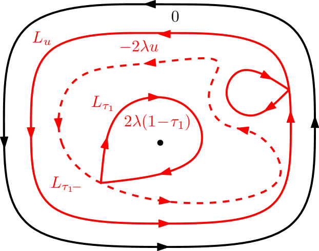
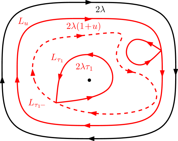
Proposition 3.2.4.
In the coupling between and càdlàg sequence of quasisimple loops as in Proposition 3.2.3, the sequence of loops is almost surely determined by the field .
Proof.
First, we show that, for any and , let be the level loop of with height for some , then stays outside of which is the connected component of that contains the origin. By the coupling in Proposition 3.2.3, we know that, given , the conditional law of restricted to is the same as with boundary value . If enters , then the pieces of in are level lines of with height . Whereas , this contradicts with Lemma 2.2.1 Item (1).
For each , let be the upward height-varying sequence of level loops of with height difference , where is the transition step. We reindex the sequence in the following way:
We use the same notations as in Remark 3.2.2.
Second, we show that, for any and , the loop almost surely coincides with and hence the loop is almost surely determined by . We have the following observations.
- (a)
-
(b)
The loop has the same law as .
Combining these two facts, we have that and coincide.
Third, we show that, for any and , the loop almost surely coincides with and hence the loop is almost surely determined by . This is true because .
Fourth, we show that, for any , the loop coincides with and is almost surely determined by ; and that, the loop coincides with and is almost surely determined by . We only show the conclusion for and the conclusion for can be proved similarly.
Assume that for some integer , define . We can prove by induction on that is almost surely determined by . When , since , the conclusion holds by the third step. Suppose that the conclusion holds for , consider the loop , we have the following observations.
-
(a)
The loop is almost surely determined by . Let be the connected component of that contains the origin. We also know that the conditional law of restricted to is the same as with boundary value .
-
(b)
The sequence is coupled with in the same way as in Proposition 3.2.3, thus is almost surely determined by by the third step.
Combining these two facts, we have that is almost surely determined by .
Finally, we show that, the loop is almost surely determined by . By the fourth step, we know that, for any , the loop coincides with . Therefore, . Whereas, the quantity has the same law as , thus almost surely. We will argue that stays outside of . Assume this is true, then we know that the limit stays outside of . Combining with the fact that has the same law as , we know that coincides with and hence it is almost surely determined by . Thus, we only need to show that stays outside of . We have the following observations.
-
(a)
By the coupling in Proposition 3.2.3, we know that, the conditional law of restricted to is the same as with boundary value .
-
(b)
The loop is a level loop of with height .
-
(c)
We know that .
Combining these three facts, if enters , then the pieces of in are level lines of with height . Whereas, , this contradicts with Lemma 2.2.1 Item (1). ∎
In the coupling given by Proposition 3.2.3, we call the sequence of quasisimple loops the upward continuum exploration process of targeted at the origin. The following proposition describes the target-independence of the continuum exploration process.


Proposition 3.2.5.
Suppose that is a zero-boundary on . Fix two target points . Let (resp. ) be the upward continuum exploration process of targeted at (resp. targeted at ). Define stopping times: (with the convention that )
Then, almost surely, we have ; moreover, the loops and coincide for all .
Proof.
First, we show the conclusion for the case . This is the case that is contained in . In this case, we have that the sequence is coupled with in the same way as the upward continuum exploration process targeted at . By Proposition 3.2.4, we have that the two sequences and coincide. In particular .
Next, we show the conclusion for the case . Let be any -stopping time such that . Note that the sequence is coupled with in the same way as the upward continuum exploration process targeted at stopped at . Combining with Proposition 3.2.4, we know that the two sequences and coincide. This holds for any . In particular, for any , we have . We only need to show that .
Consider the relation between and , there are two possibilities: the two loops are disjoint (see Figure 3.2.2(a))or the two loops coincide (see Figure 3.2.2(b)(c)). In the former case, clearly, we have . In the latter case, let us consider the relation between and . If the loop has the same orientation as (Figure 3.2.2(b)), then at time , the loop disconnects from by attaching a bubble that surrounds to . This implies that is exactly this bubble, thus . If the loop has the different orientation from (Figure 3.2.2(c)), in other words , then at time , the loop is a bubble attaching to that disconnects from . This implies that is the union of and . Thus . ∎
From Proposition 3.2.5, we see that two upward continuum exploration processes with distinct target points coincide up to the first disconnecting time. In fact, in [WW13, Lemma 8], the authors prove that the two processes (constructed from Poisson point process of -bubbles): and have the same law up to the first disconnecting time, and hence can be coupled so that they coincide up to the first disconnecting time. By Proposition 3.2.5, we see that provides exactly this coupling. Namely, we couple the two processes with the same so that is the upward continuum exploration process of targeted at and is the upward continuum exploration process of targeted at . Then the two processes almost surely coincide up to the first disconnecting time.
Now we can consider the upward continuum exploration processes of targeted at all points in simultaneously. Note that, for each pair of points , the process targeted at and the process targeted at coincide up to the first disconnecting time. We summarize some properties of the process in the following.
Proposition 3.2.6.
Suppose that is a zero-boundary on .
-
(1)
The upward continuum exploration processes targeted at all points in are almost surely determined by .
-
(2)
The law of the upward continuum exploration processes targeted at all points in is invariant under any Möbius transformation of .
-
(3)
The collection of all clockwise loops in the upward continuum exploration processes targeted at all points in has the same law as in .
3.3 Alternating continuum exploration process of
In this section, we will describe an alternating continuum exploration process which can be viewed as the limit of the alternating height-varying sequence of level loops as the height difference goes to zero. Before this, let us summarize what we have obtained by now.
Suppose that is a Poisson point process with -bubble measure . Let be the first time that surrounds the origin. Define
-
(a)
From Section 3.1, we can map the bubbles one-by-one into the unit disc and obtain a càdlàg sequence of quasisimple loops . We give the counterclockwise orientation to the loops for ; and the clockwise orientation to the loop . The loop has the same law as the loop in that surrounds the origin.
-
(b)
From Section 3.2, we know that there exists a coupling between zero-boundary and the sequence such that, for any stopping time , the conditional law of given is the same as with certain boundary value. Moreover, in this coupling, the sequence of loops is almost surely determined by the field.
In this construction, we call the sequence of loops the upward continuum exploration process of starting from (counterclockwise) targeted at the origin. See Figure 3.2.1 (a). Symmetrically, we can also construct the downward continuum exploration process of a with boundary value in starting from (clockwise) targeted at the origin. See Figure 3.2.1(b). Note that, for the downward continuum exploration process , we have that, for any stopping time , the conditional law of given is the same as whose boundary value is
In particular, for any stopping time , the conditional law of , given , restricted to the connected component of that contains the origin is the same as with boundary value . The conditional law of , given , restricted to is the same as with boundary value .
Now we can construct alternating continuum exploration process going all the way to the origin. Suppose that is a zero-boundary on and is oriented counterclockwise. We start by the upward continuum exploration process which can be viewed as being constructed from . Given , the conditional law of restricted to is the same as with boundary value . We continue the process by the downward continuum exploration process of restricted to : . This process can be viewed as being constructed from . Given , the conditional law of restricted to is the same as with boundary value .
Generally, given for some , we continue the sequence by the upward continuum exploration process and then continue the sequence by the downward continuum exploration process .
In this way, we obtain a sequence of quasisimple loops which we call the alternating continuum exploration process of starting from targeted at the origin. We call the sequence of transition times. For the sequence of transition times, we have the following.
-
(a)
For , the loops have the same orientation for , which is different from .
-
(b)
The random variables are i.i.d. with exponential law.
We summarize some basic properties of the alternating continuum exploration process of in the following proposition.
Proposition 3.3.1.
Suppose that is the alternating continuum exploration process of a zero-boundary . Then we have the following.
-
(1)
The sequence is almost surely càdlàg and transient.
-
(2)
The sequence is almost surely determined by .
-
(3)
The sequence satisfies domain Markov property: for any stopping time , let be the connected component of that contains the origin, and let be the conformal map from onto with and . Then the sequence has the same law as the alternating continuum exploration process of .
Proof.
Lemma 3.1.1 implies that the sequence is càdlàg; Proposition 3.2.4 implies that the sequence is almost surely determined by the field; and the domain Markov property is immediate from the construction. We only need to explain that the sequence is transient.
Note that has the same law as the loop in that surrounds the origin. In particular, and there exist and such that
Then the transience can be proved similarly as the proof of Proposition 2.2.6. ∎
By Proposition 3.2.5, we have the following target-independence property of the alternating continuum exploration process.
Proposition 3.3.2.
Suppose that is a zero-boundary in . Fix two target points . For , let be the alternating continuum exploration process of starting from targeted at ; and denote by the connected component of that contains . Then there exists a number such that
Given , the two processes continue towards their target points respectively in a conditionally independent way.
Suppose that is a zero-boundary on and is the alternating continuum exploration process of targeted at where is the sequence of transition times. We know that the loop has the same law as the loop in in that surrounds . By domain Markov property, we know that the sequence has the same law as the sequence of loops in nested in that surrounds .
From Proposition 3.3.2, we know that the two alternating continuum exploration processes of with distinct target points coincide up to the first disconnecting time. Let us consider the alternating continuum exploration processes of targeted at all points in simultaneously. We summarize some properties of this process in the following proposition.
Proposition 3.3.3.
Suppose that is a zero-boundary in . For each , let be the alternating continuum exploration process targeted at and let be the sequence of transition times.
-
(1)
The alternating continuum exploration processes targeted at all points in are almost surely determined by .
-
(2)
The law of the alternating continuum exploration processes targeted at all points in is invariant under any Möbius transformation of .
-
(3)
The collection of loops in the alternating continuum exploration processes targeted at all points in has the same law as nested in .
In the coupling as in Theorem 1.2.1, we call the sequence the alternating continuum exploration process of starting from the origin targeted at infinity when (resp. starting from targeted at when ).
3.4 Interaction
The following proposition describes the interaction between the continuum exploration process and the level line of , it can be proved similarly as the proof of Proposition 2.3.1.
Proposition 3.4.1.
Fix a domain with harmonically non-trivial boundary. Fix three points and . Let be a on , let be the alternating continuum exploration process of starting from targeted at , and let be the level line of with height starting from targeted at . For any -stopping time , assume that the loop does not hit and has boundary value to the left-side and to the right-side. On the event , we have that
Moreover, the level line stays outside of .
The following proposition describes the interaction between two alternating continuum exploration processes with distinct starting points.

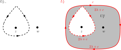
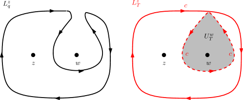
Proposition 3.4.2.
Let be a whole-plane modulo a global additive constant in . Fix two starting points and . Let (resp. ) be the alternating continuum exploration process of starting from (resp. starting from ) targeted at . Define stopping times
Then, almost surely, the quasisimple loops and coincide.
Proof.
We will argue that is contained in the closure of . If this is true, then by symmetry, the loop is contained in the closure of . Combining these two facts, the two loops and have to be equal.
We may assume that is clockwise and the case that is counterclockwise can be proved similarly. We assume that has boundary value to the left-side and to the right-side. There are three possibilities for the relation between and :
Let be the connected component of that contains . From the coupling between and the sequence , we have the following.
-
(a)
Given , the conditional law of restricted to is the same as with boundary value .
-
(b)
Given , the conditional law of restricted to is the same as with boundary value
Fix some so that is contained in . Consider the field restricted to . Given , the conditional law of restricted to is the same as and the process is the alternating continuum exploration process of targeted at . For each , let be the alternating height-varying sequence of level loops of with height difference starting from targeted at . Let be the first such that disconnects from . We know that the loop almost surely converges to in Carathéodory topology seen from as goes to . Therefore, in order to show that is contained in the closure of , it is sufficient to show that, for each large enough, the loop is contained in the closure of . We prove this case by case.
Case 1. Consider the sequence . Let be the first that exits . Assume that the level loop has height . We have the following observations.
-
(a)
Since the loops and have nonempty intersection, the loop has nonempty intersection with .
-
(b)
The pieces of that are outside of are level lines of with height , thus by Lemma 2.2.1 Item (1).
-
(c)
For each such that , let be the level loop of with height targeted at . Clearly, disconnects both and from .
Combining these three facts with Lemma 2.2.3, we know that coincides with . Consequently, the loop is the first loop in that disconnects from and it is contained in the closure of .
Case 2. Consider the sequence . Let be the first that exits . Assume that the level loop has height . If has non-trivial pieces in , then the same argument for Case 1 would show that is the first loop in that disconnects from and it is contained in the closure of . In fact, it is impossible that . We will prove it by contradiction. Assume that . We have the following observations.
-
(a)
The loop can hit from the inside, this implies that by Lemma 2.2.1 Item (3).
-
(b)
Consider the field restricted to , it has boundary value . For any such that , let be the level loop with height . Clearly, it is contained in .
Combining these two facts, the loop has to coincide with . This contradicts with the fact that exits .
Case 3. Let be any -stopping time such that . We have the following observations.
-
(a)
Recall that is the alternating height-varying sequence of level loops of and that is the first such that disconnects from .
-
(b)
the sequence is coupled with in the same way as in Theorem 1.2.1 stopped at .
Combining these two facts with Proposition 3.4.1, we have that each loop in stays outside of . In particular, the loop is contained in the closure of .
Consider the field restricted to , for , let be the alternating height-varying sequence of level loops of with height difference starting from targeted at . Let be the first that disconnects from . We can see that, for fixed and for large enough, the loop is contained in the closure of . As goes to , this implies that the loop is contained in the closure of . This completes the proof. ∎
Proof of Theorem 1.2.3.
Proof of Theorem 1.2.2.
Proof of Theorem 1.2.4.
3.5 Reversibility
In this section, we will complete the proof of Theorem 1.2.6 and derive some consequences.
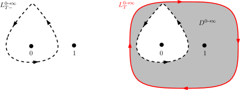
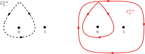
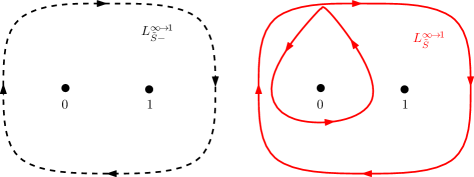
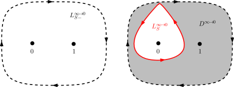
Lemma 3.5.1.
Suppose that is a whole-plane modulo a global additive constant in . Let be the alternating continuum exploration process of starting from the origin targeted at . Define to be the first time that disconnects from . Define to be the event that the loop does not disconnect from and that is a transition time (see Figure 3.5.1(a)). On the event , define to be the domain between the loop and the loop :
Similarly, we can define the event and the domain for the alternating continuum exploration process of starting from targeted at the origin. Then, almost surely on the event , the event also holds and the regions and coincide.
Proof.
For , we denote by the alternating continuum exploration process of starting from targeted at . Define
We have the following observations.
- (a)
- (b)
- (c)
Combining these three facts, we have that, almost surely on , the event holds and that the regions and coincide. ∎
Remark 3.5.2.
Assume the same notations as in Lemma 3.5.1, we have the following consequences.
-
(a)
Both the loops and are simple loops.
-
(b)
Consider the compact set , its interior is simply connected and its complement in the Riemann sphere has two connected components: one contains the origin and the other one contains .
Proof of Theorem 1.2.6.
We only need to show that the two unions of transition regions coincide, and this implies that the two unions of stationary regions coincide.
For any , suppose that is contained in the interior of . Since is a sequence of compact sets with disjoint interiors, there is exactly one that contains . By Lemma 3.5.1, there exists that contains ; moreover, the region coincides with . This implies that the union is contained in the union . Combining with the symmetry, the two unions coincide. ∎
Suppose that is a whole-plane modulo a global additive constant in . Let be the alternating continuum exploration process of starting from the origin targeted at where is the sequence of transition times. Let (resp. ) be the sequence of transition regions (resp. the sequence of stationary regions) of starting from the origin targeted at . From Remark 3.5.2, we have the following observations.
-
(a)
For each transition time , the loops and are simple loops.
-
(b)
For each , the interior of is simply connected, and the complement of in the Riemann sphere has two connected components: one contains the origin and the other one contains .
-
(c)
For each , the complement of in the Riemann sphere has two connected components: one contains the origin and the other one contains . (The interior of is an annulus when the loops and are disjoint, or is not connected when the loops and have non-empty intersection.)
-
(d)
The complement of the union is the union of interiors of .
References
- [Law05] Gregory F. Lawler. Conformally invariant processes in the plane, volume 114 of Mathematical Surveys and Monographs. American Mathematical Society, Providence, RI, 2005.
- [MS12] Jason Miller and Scott Sheffield. Imaginary Geometry III: Reversibility of SLEκ for . 2012.
- [MS13] Jason Miller and Scott Sheffield. Imaginary Geometry IV: Interior Rays, Whole-plane Reversibility, and Space-filling Trees. 2013.
- [MS16a] Jason Miller and Scott Sheffield. Imaginary geometry I: interacting SLEs. Probab. Theory Related Fields, 164(3-4):553–705, 2016.
- [MS16b] Jason Miller and Scott Sheffield. Imaginary geometry II: Reversibility of for . Ann. Probab., 44(3):1647–1722, 2016.
- [She09] Scott Sheffield. Exploration trees and conformal loop ensembles. Duke Math. J., 147(1):79–129, 2009.
- [SS09] Oded Schramm and Scott Sheffield. Contour lines of the two-dimensional discrete Gaussian free field. Acta Math., 202(1):21–137, 2009.
- [SS13] Oded Schramm and Scott Sheffield. A contour line of the continuum Gaussian free field. Probab. Theory Related Fields, 157(1-2):47–80, 2013.
- [SW12] Scott Sheffield and Wendelin Werner. Conformal loop ensembles: the Markovian characterization and the loop-soup construction. Ann. of Math. (2), 176(3):1827–1917, 2012.
- [SWW16] Scott Sheffield, Samuel Watson, and Hao Wu. Simple cle in doubly connected domains. Annales de l’Institut Henri Poincare, page to appear, 2016.
- [WW13] Wendelin Werner and Hao Wu. On Conformally Invariant CLE Explorations. Comm. Math. Phys., 320(3):637–661, 2013.
- [WW16] Menglu Wang and Hao Wu. Level Lines of Gaussian Free Field I: Zero-Boundary GFF. Stochastic Processes and their Applications, page to appear, 2016.
Menglu Wang
Department of Mathematics, Massachusetts Institute of Technology, Cambridge, MA, USA
mengluw@math.mit.edu
Hao Wu
NCCR/SwissMAP, Section de Mathématiques, Université de Genève, Switzerland
and
Yau Mathematical Sciences Center, Tsinghua University, China
hao.wu.proba@gmail.com