On short recurrence Krylov type methods for linear systems with many right-hand sides

Abstract

Block and global Krylov subspace methods have been proposed as methods adapted to the situation where one iteratively solves systems with the same matrix and several right hand sides. These methods are advantageous, since they allow to cast the major part of the arithmetic in terms of matrix-block vector products, and since, in the block case, they take their iterates from a potentially richer subspace. In this paper we consider the most established Krylov subspace methods which rely on short recurrencies, i.e. BiCG, QMR and BiCGStab. We propose modifications of their block variants which increase numerical stability, thus at least partly curing a problem previously observed by several authors. Moreover, we develop modifications of the “global” variants which almost halve the number of matrix-vector multiplications. We present a discussion as well as numerical evidence which both indicate that the additional work present in the block methods can be substantial, and that the new “economic” versions of the “global” BiCG and QMR method can be considered as good alternatives to the BiCGStab variants.

1 Introduction

We consider simultaneous linear systems with the same matrix $A\in\mathbb{C}^{n\times n}$ and $s$ right-hand sides (r.h.s.) $b_{i}$,

$$Ax_{i}=b_{i},\;i=1,\ldots,s,$$ (1)

which we also formulate in block form as the matrix equation

$$AX=B,\;\mbox{ where }X=[x_{1}|\ldots|x_{s}],B=[b_{1}|\ldots|b_{s}]\in\mathbb{C}^{n\times s}.$$

As a general rule we will use lower case letters with sub-indices for the columns of the matrix denoted with the corresponding upper case letter.

Our overall assumption is that $A$ is large and sparse and that a (preconditioned) Krylov subspace type iterative method is to be used to iteratively approximate the solutions for the different r.h.s. Our interest is in methods which efficiently take advantage of the fact that we are given the $s$ linear systems with the r.h.s. $b_{i},i=1,\ldots,s$ simultaneously, and we use the generic name simultaneous methods for any such method. Investigations in this setting are not new, the development and analysis of block variants of the standard Krylov subspace methods dating back to at least the mid 1980s [23]. With the advent of massively parallel processor architectures such as GPUs, where memory access is usually the determining factor for computational speed, simultaneous linear systems of the form (1) offer the possibility of optimizing memory access to $A$ by reading and storing $A$ only once while updating the iterates for all $s$ r.h.s. simultaneously. Algorithms which take this into account can therefore be expected to run faster because their arithmetic operations perform faster. Moreover, simultaneous methods also offer the potential to, in addition, increase the speed of convergence when obtaining their iterates from a larger, “block” Krylov subspace rather than the standard Krylov subspaces.

As a rule of thumb, working with $s$ several r.h.s. simultaneously instead of just one increases the number of vectors to be stored by a factor of $s$. This is why simultaneous variants of the GMRES method may, due to the long recurrences present in GMRES, suffer from the fact that the method has to be restarted after a relatively small number of iterations. This typically degrades the speed of convergence.

In this paper we therefore focus on simultaneous Krylov type methods relying on short recurrences. We assume that $A$ is a general non-singular matrix, i.e. we do not assume that we can take advantage of additional properties of $A$ like symmetry, e.g. Typical and well-established methods for a single right-hand side in this case are BiCG (bi-conjugate gradients [10]), BiCGStab (stabilized BiCG [32]) and QMR (quasi-minimal residual method [12]), and we mainly develop on three different simultaneous variants for each of these three methods in this paper. In section 2 we introduce the three different principles termed loop-interchanging, global and block to generate a simultaneous variant from a given (single r.h.s.) Krylov subspace method and, as an example, describe the resulting BiCG variants in some detail. We then devote section 3 to a discussion of the various simultaneous methods known from the literature in our context before developing two improvements in section 4. One improvement reduces the arithmetic cost in the global BiCG and QMR variants by nearly a factor of 2, suppressing almost all of the matrix-vector multiplications with $A^{H}$. The other improvement enhances numerical stability in the block methods through the judicious use of QR-factorizations of the matrix of simultaneous residuals. Section 5 contains an extensive numerical study for the various methods and conclusions on which methods are to be preferred in which situations.

2 Loop-interchanging, global and block Krylov methods

In this section we describe three different approaches to obtain a simultaneous Krylov subspace method for $s$ r.h.s. from a given method for a single r.h.s. All resulting simultaneous methods reduce to the single r.h.s. method for $s=1$.

Solving the systems (1) one after the other with the same Krylov subspace method can be viewed as performing two nested loops with the outer loop (“for $i=1,\ldots,s$”) running over the different r.h.s. and the inner loop (“for $k=1,\ldots$ until convergence”) performing the iteration of the Krylov subspace method. These two loops can be interchanged, resulting in an algorithm where each sweep through the inner loop can be organized in a way such that all occurring matrix-vector multiplications for all $i$ are gathered into one matrix-block-vector multiplication, the term “block vector” denoting a matrix of size $n\times s$. For BiCG as the underlying single r.h.s. Krylov subspace method, Algorithm 1 states the resulting Li-BiCG method, where Li stands for “loop interchanged”. Note that whenever possible we cast inner loop operations as operations with $n\times s$ matrices with, e.g., column $x_{i}^{(k)}$ of $X^{(k)}\in\mathbb{C}^{n\times s}$ being the BiCG iterate for the r.h.s. $b_{i}$, etc. The inner loop index appears explicitly only when calculating the $i$-th diagonal entries $\alpha_{i}^{(k)}$ and $\beta_{i}^{(k)}$ of the $s\times s$ diagonal matrices ${\rm diag}(\alpha^{(k)})$ and ${\rm diag}(\beta^{(k)})$, respectively. All multiplications with the matrices $A$ and $A^{H}$ appear as matrix-block-vector multiplications $AP^{(k)}$ and $A^{H}\hat{P}^{(k)}$. If the nominator in the definition of $\alpha_{i}^{(k)}$ or $\beta_{i}^{(k)}$ is zero, the iteration for r.h.s. $b_{i}$ breaks down.

choose $X^{(0)},\hat{R}^{(0)}\in\mathbb{C}^{n\times s}$

put $R^{(0)}=B-AX^{(0)},\,P^{(0)}=R^{(0)},\hat{P}^{(0)}=\hat{R}^{(0)}$

for $k=0,1,2,\dots$ until convergence do

       $Q^{(k)}=AP^{(k)}$

       $\alpha_{i}^{(k)}=\langle r_{i}^{(k)},\hat{r}_{i}^{(k)}\rangle/\langle q_{i}^{(k)},\hat{p}_{i}^{(k)}\rangle,\;i=1,\ldots,s$

       $X^{(k+1)}=X^{(k)}+P^{(k)}{\rm diag}(\alpha^{(k)})$

       $R^{(k+1)}=R^{(k)}-Q^{(k)}{\rm diag}(\alpha^{(k)}),\;\hat{R}^{(k+1)}=\hat{R}^{(k)}-(A^{H}\hat{P}^{(k)})\overline{{\rm diag}(\alpha^{(k)})}$

       $\beta_{i}^{(k)}=\langle r_{i}^{(k+1)},\hat{r}_{i}^{(k+1)}\rangle/\langle r_{i}^{(k)},\hat{r}_{i}^{(k)}\rangle,\;i=1,\ldots,s$

       $P^{(k+1)}=R^{(k+1)}+P^{(k)}{\rm diag}(\beta^{(k)}),\;\hat{P}^{(k+1)}=\hat{R}^{(k+1)}+\hat{P}^{(k)}\overline{{\rm diag}(\beta^{(k)})}$

Algorithm 1 Loop-interchanged BiCG (Li-BiCG)

Global methods take a different approach. They cast the $s$ systems (1) into one big, tensorized $sn\times sn$ system

$$(I\otimes A)x=b,\mbox{ where }b=\left[\begin{array}[]{c}b_{1}\\ \vdots\\ b_{s}\end{array}\right],\,x=\left[\begin{array}[]{c}x_{1}\\ \vdots\\ x_{s}\end{array}\right],$$ (2)

and then apply a standard Krylov subspace method to the system (2). Using the $\textrm{mat}_{m\times s}$ operator to cast vectors $x$ of length $ns$ into matrices $X$ of size $n\times s$ “by columns”, i.e. $(X)_{ij}=x_{(j-1)n+i}$, and the identities

$$\textrm{mat}_{n\times s}((I\otimes A)x)=AX,\enspace\langle x,y\rangle=\textrm{tr}(Y^{H}X)\enspace\mbox{ where}$$

$$X=\textrm{mat}_{n\times s}(x),Y=\textrm{mat}_{n\times s}(y),$$

we end up with the formulation of BiCG for (2) given in Algorithm 2 known as global BiCG (Gl-BiCG), see [21]. The algorithm breaks down if the nominator in $\alpha^{(k)}$ or $\beta^{(k)}$ is zero.

choose $X^{(0)},\hat{R}^{(0)}\in\mathbb{C}^{n\times s}$

put $R^{(0)}=B-AX^{(0)},\,P^{(0)}=R^{(0)},\hat{P}^{(0)}=\hat{R}^{(0)}$

for $k=0,1,2,\dots$ until convergence do

       $Q^{(k)}=AP^{(k)}$

       $\alpha^{(k)}=\textrm{tr}((\hat{R}^{(k)})^{H}R^{(k)})/\textrm{tr}((\hat{P}^{(k)})^{H}Q^{(k)})$

       $X^{(k+1)}=X^{(k)}+\alpha^{(k)}P^{(k)}$

       $R^{(k+1)}=R^{(k)}-\alpha^{(k)}Q^{(k)},\;\hat{R}^{(k+1)}=\hat{R}^{(k)}-\overline{\alpha^{(k)}}(A^{H}\hat{P}^{(k)})$

       $\beta^{(k)}=\textrm{tr}((\hat{R}^{(k+1)})^{H}R^{(k+1)})/\textrm{tr}((\hat{R}^{(k)})^{H}R^{(k)})$

       $P^{(k+1)}=R^{(k+1)}+\beta^{(k)}P^{(k)},\;\hat{P}^{(k+1)}=\hat{R}^{(k+1)}+\overline{\beta^{(k)}}\hat{P}^{(k)}$

Algorithm 2 Global BiCG (Gl-BiCG)

In the loop interchange and the global variant of BiCG the $i$th columns $r^{(\ell)}_{i}$ for $\ell=0,\ldots,k-1$ represent a basis for the Krylov subspace

$$\mathcal{K}_{k}(A,r_{i}^{(0)})=\mbox{span}\{r_{i}^{(0)},Ar_{i}^{(0)},\ldots A^{(k-1)}r_{i}^{(0)}\},$$

and in both methods the iterate $x_{i}^{(k)}$, the $i$th column of $X^{(k)}$, is taken from $x^{(0)}_{i}+\mathcal{K}_{k}(A,r_{i}^{(0)})$. Block Krylov subspace methods take advantage of the fact that the Krylov subspaces $\mathcal{K}_{k}(A,r_{i}^{(0)}),i=1,\ldots,s$ are available simultaneously and take each iterate $x_{i}^{(k)}$ from the larger “block” Krylov subspace

$$\mathcal{K}_{k}(A,R^{(0)}):=\sum_{i=1}^{s}\mathcal{K}_{k}(A,r_{i}^{(0)}),$$

which has dimension $sk$ (or less if linear dependence occurs “across” the single r.h.s. Krylov subspaces $\mathcal{K}_{k}(A,r_{i}^{(0)})$). The usual approach is to transfer the variational characterization for the iterates of the single r.h.s. method to the block Krylov subspace. In this manner, the block BiCG method from [23] defines its iterates $X^{(k)}$ (they appear again as the columns of an $n\times s$ block vector) by requiring that the iterates $x_{i}^{(k)}$ are from $x_{i}^{(0)}+\mathcal{K}_{k}(A,R^{(0)})$ and their residuals are orthogonal to $\mathcal{K}_{k}(A^{H},\hat{R}^{(0)})$ for some “shadow residual” block vector $\hat{R}^{(0)}\in\mathbb{C}^{n\times s}$. The resulting method Bl-BiCG (block BiCG), is given as Algorithm 3. Note that now the quantities $\alpha^{(k)},\hat{\alpha}^{(k)},\beta^{(k)}$ and $\hat{\beta}^{(k)}$ are $s\times s$-matrices, and the method breaks down prematurely if one of the matrices $(P^{(k)})^{H}A^{H}\hat{P}^{(k)},(\hat{R}^{(k)})^{H}R^{(k)}$ is singular.

choose $X^{(0)},\hat{R}^{(0)}\in\mathbb{C}^{n\times s}$

put $R^{(0)}=B-AX^{(0)},\,P^{(0)}=R^{(0)},\hat{P}^{(0)}=\hat{R}^{(0)}$

for $k=0,1,2,\dots$ until convergence do

       $Q^{(k)}=AP^{(k)},\;\hat{Q}^{(k)}=A^{H}\hat{P}^{(k)}$

       $\alpha^{(k)}=\big{(}(\hat{P}^{(k)})^{H}Q^{(k)}\big{)}^{-1}\big{(}(\hat{R}^{(k)})^{H}R^{(k)}\big{)}$

       $\hat{\alpha}^{(k)}=\big{(}(P^{(k)})^{H}\hat{Q}^{(k)}\big{)}^{-1}\big{(}({R}^{(k)})^{H}\hat{R}^{(k)}\big{)}$

       $X^{(k+1)}=X^{(k)}+P^{(k)}\alpha^{(k)}$

       $R^{(k+1)}=R^{(k)}-Q^{(k)}\alpha^{(k)},\;\hat{R}^{(k+1)}=\hat{R}^{(k)}-\hat{Q}^{(k)}\hat{\alpha}^{(k)}$

       $\beta^{(k)}=\big{(}(\hat{R}^{(k)})^{H}R^{(k)}\big{)}^{-1}\big{(}(\hat{R}^{(k+1)})^{H}R^{(k+1)}\big{)}$

       $\hat{\beta}^{(k)}=\big{(}({R}^{(k)})^{H}\hat{R}^{(k)}\big{)}^{-1}\big{(}({R}^{(k+1)})^{H}\hat{R}^{(k+1)}\big{)}$

       $P^{(k+1)}=R^{(k+1)}+P^{(k)}\beta^{(k)},\;\hat{P}^{(k+1)}=\hat{R}^{(k+1)}+\hat{P}^{(k)}\hat{\beta}^{(k)}$

Algorithm 3 Block BiCG (Bl-BiCG)

Apart from the matrix-vector multiplications, the work to update the various quantities is substantially higher in block BiCG as compared to loop interchanged BiCG and global BiCG. Counting an inner product or a SAXPY operation with vectors of length $n$ as one vector operation (representing $n$ additions and $n$ multiplications), we have the following proposition, the proof of which also gives an indication on how to save arithmetic work by re-using information from the previous iteration.

Proposition 1

One iteration of Li-BiCG, Gl-BiCG or Bl-BiCG requires two matrix-block-vector multiplications (one with $A$ and one with $A^{H}$) with block-vectors of size $n\times s$ plus $7s$ additional vector operations for Li-BiCG as well as Gl-BiCG, and $7s^{2}$ additional vector operations for Bl-BiCG.

Proof 1

We only have to care about operations other than the multiplications with $A$ and $A^{H}$. In Li-BiCG, assuming that we save $\langle\hat{r}_{i}^{(k+1)},r_{i}^{(k+1)}\rangle$ for re-use in the next iteration, we need a total of $2s$ inner products to compute all $\alpha_{i}^{(k)},\beta_{i}^{(k)}$ and $s$ SAXPYs for each of $X^{(k+1)}$, $R^{(k+1)}$, $\hat{R}^{(k+1)}$, $P^{(k+1)}$, $\hat{P}^{(k+1)}$. Exactly the same count holds for Gl-BiCG. In Bl-BiCG we can save $\big{(}\hat{R}^{(k+1)}\big{)}^{H}R^{(k+1)}$ for use in the next iteration, and we can exploit the fact that the two factors defining $\alpha^{(k)}$ are just the adjoints of those defining $\hat{\alpha}^{(k)}$, and similarly for $\beta^{(k)}$ and $\hat{\beta}^{(k)}$. So we need just $2s^{2}$ inner products to build these factors, and we neglect the cost $\mathcal{O}(s^{3})$ for multiplying $s\times s$ matrices. The computation of each of $X^{(k+1)}$, $R^{(k+1)}$, $\hat{R}^{(k+1)}$, $P^{(k+1)}$, $\hat{P}^{(k+1)}$ requires $s^{2}$ SAXPYs.

We note that the updates of $X^{(k+1)}$, $R^{(k+1)}$, $\hat{R}^{(k+1)}$, $P^{(k+1)}$, $\hat{P}^{(k+1)}$ in the block method actually represent BLAS3 GEMM operations, see [8] which have a more favorable ratio of memory access to arithmetic work than SAXPY operations, so the overhead of a factor of $s$ of the block method vs. the loop interchange and the global method suggested by Proposition 1 may show less in actual timings.

In a similar way one obtains the three simultaneous variants Li-QMR, Gl-QMR and Bl-QMR of the QMR method. The variational characterization in Bl-QMR is that the 2-norm of the coefficients which represent the residual from $K_{k}(A,R^{(0)})$ in the nested bi-orthogonal basis of $K_{k}(A,R^{(0)})$ with respect to $K_{k}(A^{H},\hat{R}^{(0)})$, be minimal; see [11]. We do not write down the resulting algorithms explicitly nor do we so for the BiCGStab variants Li-BiCGStab, Gl-BiCGStab and Bl-BiCGStab. It is worth mentioning, though, that BiCGStab does not have a proper variational characterization, its main property being that multiplications with $A^{H}$ present in BiCG are replaced by those with $A$, thus obtaining iterate $x^{(k)}$ from $x^{(0)}+\mathcal{K}_{2k}(A,r^{(0)})$ while imposing a steepest descent property on the residual as an intermediate step. The block BiCGStab method from [16] transfers this approach to the multiple r.h.s. case such that the $k$-th iterate $x_{i}^{(k)}$ is from $x_{i}^{(0)}+\mathcal{K}_{2k}(A,R^{(0)})$, imposing a condition on the residuals in the intermediate steps which, interestingly, is quite in the spirit of a “global” steepest descent method. We refer to [16] for details.

3 Discussion of the literature

The loop interchange approach is most probably not new, although we are not aware of a systematic discussion as a construction principle for simultaneous methods.

Global methods were considered in a variety of papers. Surprisingly, although they all just realize the approach to perform the respective single r.h.s. method for (2) and then “matricize” all operations with vectors of length $ns$, we could not find this fact mentioned explicitly in the literature. The first global methods are global full orthogonalization (Gl-FOM) and global generalized minimal residual (Gl-GMRES), introduced in [20]. Gl-BiCG and Gl-BiCGStab were suggested in [21], and global variants of less well-known Krylov subspace methods were subsequently proposed in [18] (Gl-CMRH), [34] (Gl-CGS), [15] (Gl-SCD) and [35] (Gl-BiCR and its variants).

Block Krylov subspace methods were introduced in [23], where Bl-BiCG was considered together with block conjugate gradients (Bl-CG). The (long recurrence) block generalized minimal residual (Bl-GMRES) algorithm goes back to [27] and [33], and a convergence analysis can be found in [28]. Block Krylov subspace methods require additional work for factorizations and multiplications of $n\times s$ or $s\times s$ matrices in each iteration (cf. Proposition 1). Very often, this substantially slows down the overall process. The hybrid method from [29] describes an approach, where this additional work is reduced by adding cycles in which a (matrix valued) polynomial obtained from the block Arnoldi process of a previous cycle is used. The additional cycles save arithmetic cost since they do not perform the block Arnoldi process.

The Bl-QMR method was suggested in [11], Bl-BiCGStab goes back to [16], and Bl-LSQR, a block least squares QR-algorithm to solve the normal equations for simultaneous r.h.s. was given in [22]. The block methods relying on the non-symmetric Lanczos process can suffer from the fact that this process can break down prematurely if the bi-orthogonality condition imposed on the to be computed block basis vectors can not be fulfilled. Numerically, this will typically result in very ill-conditioned $s\times s$ matrices in Bl-BiCG and Bl-BiCGStab for which linear systems have to be solved in the algorithm. The non-symmetric Lanczos process at the basis of Bl-QMR from [1] does, in principle, not suffer from this phenomenon since it incorporates a look-ahead strategy which cures almost all possible unwanted breakdowns. Both, the block Arnoldi process at the basis of Bl-GMRES as well as the symmetric or non-symmetric Lanczos process at the basis of Bl-CG or Bl-BiCG, Bl-QMR and Bl-BiCGStab, respectively, should account for an additional danger of producing ill-conditioned $s\times s$ systems arising because of deflation. Occurrence of deflation within a block Krylov subspace method means that while the block Krylov subspaces $\mathcal{K}_{k}(A,R^{(0)})$ or $\mathcal{K}_{k}(A^{H},\hat{R}^{(0)})$ has dimension $ks$, the next, $\mathcal{K}_{k+1}(A,R^{(0)})$ or $\mathcal{K}_{k+1}(A^{H},\hat{R}^{(0)})$, has dimension less than $(k+1)s$. Similar reductions in dimension might occur again in later iterations. In principle, deflation is advantageous, since it allows to reduce the number of matrix-vector operations per iteration. However, algorithms have to be adjusted, and additional book-keeping is necessary. Deflation in the unsymmetric block Lanczos process and the block Arnoldi process was considered in [4], the consequences for Bl-GMRES are discussed in detail in [17]. Bl-QMR from [11] and the Bl-CG variant considered in [3] address deflation by indeed explicitly reducing the dimension of the block Krylov subspaces. Interestingly, the latter two methods now work by applying the matrix-vector multiplications one at a time instead of simultaneously to a block vector, checking for deflation after each such operation. These methods can thus no longer take advantage of a possible performance gain due to multiplications of matrices with block-vectors. This is in contrast to the modifications of Bl-BiCG and Bl-CG from [23] and [9] which “hide” the possible singularity of the $s\times s$ matrices by using QR-decompositions and modified update formulae. This approach to treat deflation implicitly does not allow to save matrix-vector multiplications when deflation occurs, but keeps the advantage of relying on matrix-block-vector multiplications. It does not require any additional book-keeping. Recently, in [2] a variant of Bl-CG was developed which treats deflation explicitly, but still uses matrix-block-vector multiplications.

A round-off error analysis for Bl-BiCGStab in [31] lead the authors to suggest a numerically more stable modification which basically interchanges the minimization step and the BiCG step present in each iteration of Gl-BiCGStab. A numerically more stable variant of Bl-BiCG which enforces $A$-orthogonality between the individual vectors and not just between block vectors, and which contains an additional QMR-type stabilization step, was considered in [26].

4 Improvements: Cost and stability

In any of the three simultaneous BiCG methods we are free to choose $\hat{R}^{(0)}$, the initial block-vector of shadow residuals, popular choices being $\hat{R}^{(0)}=R^{(0)}$ or $\hat{R}^{(0)}=\overline{R^{(0)}}$. If we take $\hat{R}^{(0)}$ to have identical columns, i.e.

$$\hat{R}^{(0)}=\hat{r}^{(0)}\mathbf{1}^{T},\mbox{ where }\hat{r}^{(0)}\in\mathbb{C}^{n},\;\mathbf{1}=(1,\ldots,1)^{T}\in\mathbb{C}^{s},$$

we see that in Gl-BiCG (Algorithm 2) all “shadow” block vectors $\hat{P}^{(k)}$ and $\hat{R}^{(k)}$ conserve this structure for all $k$, i.e.

$$\hat{P}^{(k)}=\hat{p}^{(k)}\mathbf{1}^{T},\;\hat{R}^{(k)}=\hat{r}^{(k)}\mathbf{1}^{T},\enspace\hat{p}^{(k)},\hat{r}^{(k)}\in\mathbb{C}^{n}.$$

A comparable situation occurs neither in Li-BiCG nor in Bl-BiCG. Only in Gl-BiCG can we therefore take advantage of an initial shadow residual with identical columns and just compute the vectors $\hat{p}^{(k)}$ and $\hat{r}^{(k)}$ rather than the respective block vectors in iteration $k-1$. In particular, we then need to multiply $A^{H}$ only with a single vector instead of a whole block vector with $s$ columns. The resulting “economic” version eGl-BiCG of Gl-BiCG is given as Algorithm 4, where we used the sum-operator to denote the sum of all components of a (row) vector and the relation $\textrm{tr}(\mathbf{1}\hat{r}^{H}R)=\textrm{sum}(\hat{r}^{H}R)$ for $\mathbf{1}\in\mathbb{C}^{s},\hat{r}\in\mathbb{C}^{n},R\in\mathbb{C}^{n\times s}$.

choose $X^{(0)}\in\mathbb{C}^{n\times s},\;\hat{r}^{(0)}\in\mathbb{C}^{n}$

put $R^{(0)}=B-AX^{(0)},\,P^{(0)}=R^{(0)},\hat{p}^{(0)}=\hat{r}^{(0)}$

for $k=0,1,2,\dots$ until convergence do

       $Q^{(k)}=AP^{(k)}$

       $\alpha^{(k)}=\textrm{sum}((\hat{r}^{(k)})^{H}R^{(k)})/\textrm{sum}((\hat{p}^{(k)})^{H}Q^{(k)})$

       $X^{(k+1)}=X^{(k)}+\alpha^{(k)}P^{(k)}$

       $R^{(k+1)}=R^{(k)}-\alpha^{(k)}Q^{(k)},\;\hat{r}^{(k+1)}=\hat{r}^{(k)}-\overline{\alpha^{(k)}}(A^{H}\hat{p}^{(k)})$

       $\beta^{(k)}=\textrm{sum}((\hat{r}^{(k+1)})^{H}R^{(k+1)})/\textrm{sum}((\hat{r}^{(k)})^{H}R^{(k)})$

       $P^{(k+1)}=R^{(k+1)}+\beta^{(k)}P^{(k)},\;\hat{p}^{(k+1)}=\hat{r}^{(k+1)}+\overline{\beta^{(k)}}\hat{p}^{(k)}$

Algorithm 4 Economic global BiCG (eGl-BiCG)

In a similar way, we obtain an economic version, eGl-QMR, of the global QMR method. There is no such opportunity for Gl-BiCGStab, where multiplications with $A^{H}$ are not present anyway. In the economic global methods the work to be performed for the shadow residuals and search directions is identical to that for just one single r.h.s., so that it becomes increasingly negligible for larger values of $s$, $s\gtrapprox 10$ say. In this manner, the economic global methods eliminate one of the important disadvantages of the short recurrence Krylov subspace methods based on the non-symmetric Lanczos process, and we will see in the numerical experiments that eGl-BiCG and eGl-QMR perform favorably when compared with simultaneous BiCGStab variants, for example.

Deflation in Bl-BiCG occurs if at some iteration $k$ one of the block vectors $P^{(k)},\hat{P}^{(k)},R^{(k)},$ and $\hat{R}^{(k)}$ becomes rank deficient, even though one might have taken care for this not to happen in iteration 0. In practice, exact deflation happens rarely, but if one of the block vectors is almost rank deficient (inexact deflation), some of the matrices $\alpha^{(k)},\hat{\alpha}^{(k)},\beta^{(k)},$ and $\hat{\beta}^{(k)}$ will be computed inaccurately, resulting in numerical instabilities of the algorithm. Already in [23] it was therefore proposed to use a QR factorization of the search direction block vectors $P^{(k)}$ and $\hat{P}^{(k)}$ to avoid such instabilities. A systematic study of different other remedies was presented in [9] for the Hermitian positive definite case, i.e., for the block CG method, and it turned out that the variant which uses a QR factorization of the residual block vectors is most convenient. This approach can be transported to block BiCG, and we performed a series of numerical comparisons which shows that also in the non-Hermitian case the variant which relies on a QR factorization of the block residuals is to be preferred over the one with QR-factorization of the block search vectors.

To precisely describe the resulting variant of block BiCG, consider a (thin) QR-factorization of the block residuals in Bl-BiCG (Algorithm 3),

$$R^{(k)}={Q}^{(k)}{C}^{(k)},\quad\hat{R}^{(k)}={\hat{Q}}^{(k)}{\hat{C}}^{(k)},$$ (3)

where

$$Q^{(k)},\hat{Q}^{(k)}\in\mathbb{C}^{n\times s},\enspace(Q^{(k)})^{H}Q^{(k)}={(\hat{Q}^{(k)})}^{H}\hat{Q}^{(k)}=I,\enspace C^{(k)},\hat{C}^{(k)}\in\mathbb{C}^{s\times s}.$$

A possible ill-conditioning of $R^{(k)}$ or $\hat{R}^{(k)}$ translates into an ill-conditioned matrix $C^{(k)}$ or $\hat{C}^{(k)}$, respectively, and Bl-BiCG can now be stabilized by using the QR-factorizations (3) while at the same time avoiding the occurrence of $(C^{(k)})^{-1}$ and $(\hat{C}^{(k)})^{-1}$. To do so, we represent the search direction block vectors $P^{(k)}$ and $\hat{P}^{(k)}$ as

$$P^{(k)}=V^{(k)}C^{(k)},\quad\hat{P}^{(k)}=\hat{V}^{(k)}\hat{C}^{(k)}.$$

For the update of the block vectors $V^{(k)}$ and $\hat{V}^{(k)}$ from Algorithm 3 we then get

$$V^{(k+1)} = Q^{(k+1)}+V^{(k)}\big{(}C^{(k)}\beta^{(k)}(C^{(k+1)})^{-1}\big{)},$$

$$\hat{V}^{(k+1)} = \hat{Q}^{(k+1)}+\hat{V}^{(k)}\big{(}\hat{C}^{(k)}\hat{\beta}^{(k)}(\hat{C}^{(k+1)})^{-1}\big{)},$$

and using (3) in the update for the block residuals we obtain

$$Q^{(k+1)}C^{(k+1)}{(C^{(k)})}^{-1} = Q^{(k)}-AV^{(k)}\big{(}C^{(k)}\alpha^{(k)}(C^{(k)})^{-1}\big{)},$$

$$\hat{Q}^{(k+1)}\hat{C}^{(k+1)}{(\hat{C}^{(k)})}^{-1} = \hat{Q}^{(k)}-A^{H}\hat{V}^{(k)}\big{(}\hat{C}^{(k)}\hat{\alpha}^{(k)}(\hat{C}^{(k)})^{-1}\big{)}.$$

This shows that computationally we can obtain $S^{(k+1)}=C^{(k+1)}{(C^{(k)})}^{-1}$ together with $Q^{(k+1)}$ from a QR factorization of $Q^{(k)}-AV^{(k)}\big{(}C^{(k)}\alpha^{(k)}(C^{(k)})^{-1}\big{)}$, and similarly for the “shadow” block vectors. Moreover, we have

$$C^{(k)}\alpha^{(k)}(C^{(k)})^{-1} = C^{(k)}\big{(}(\hat{P}^{(k)})^{H}AP^{(k)}\big{)}^{-1}\big{(}(\hat{R}^{(k)})^{H}R^{(k}\big{)}{(C^{(k)})}^{-1}$$ (4)

$$= \big{(}(\hat{V}^{(k)})^{H}AV^{(k)}\big{)}^{-1}\big{(}(\hat{Q}^{(k)})^{H}Q^{(k}\big{)},$$

and, analogously,

$$\hat{C}^{(k)}\hat{\alpha}^{(k)}(\hat{C}^{(k)})^{-1} = \big{(}({V}^{(k)})^{H}A^{H}\hat{V}^{(k)}\big{)}^{-1}\big{(}({Q}^{(k)})^{H}\hat{Q}^{(k)}\big{)},$$ (5)

$$C^{(k)}\beta^{(k)}(C^{(k+1)})^{-1} = \big{(}(\hat{Q}^{(k)})^{H}Q^{(k)}\big{)}^{-1}(\hat{S}^{(k+1)})^{H}\big{(}(\hat{Q}^{(k+1)})^{H}Q^{(k+1)}\big{)},$$ (6)

$$\hat{C}^{(k)}\hat{\beta}^{(k)}(\hat{C}^{(k+1)})^{-1} = \big{(}({Q}^{(k)})^{H}\hat{Q}^{(k)}\big{)}^{-1}(S^{(k+1)})^{H}\big{(}({Q}^{(k+1)})^{H}\hat{Q}^{(k+1)}\big{)}.$$ (7)

Putting things together, we arrive at the block BiCG algorithm using QR-factorization of the block residual, termed Bl-BiCG-rQ, given as Algorithm 5.

choose $X^{(0)},\hat{R}^{(0)}\in\mathbb{C}^{n\times s}$

put $R^{(0)}=B-AX^{(0)},\,Q^{(0)}C^{(0)}=R^{(0)},\,\hat{Q}^{(0)}\hat{C}^{(0)}=\hat{R}^{(0)},\,V^{(0)}=Q^{(0)},\hat{V}^{(0)}=\hat{Q}^{(0)}$

for $k=1,2,\dots$ until convergence do

       $W^{(k)}=AV^{(k)},\;\hat{W}^{(k)}=A^{H}\hat{V}^{(k)}$

       $\alpha^{(k)}=\big{(}(\hat{V}^{(k)})^{H}W^{(k)}\big{)}^{-1}\big{(}(\hat{Q}^{(k)})^{H}Q^{(k)}\big{)}$

       $\hat{\alpha}^{(k)}=\big{(}({V}^{(k)})^{H}\hat{W}^{(k)}\big{)}^{-1}\big{(}({Q}^{(k)})^{H}\hat{Q}^{(k)}\big{)}$

       $X^{(k+1)}=X^{(k)}+V^{(k)}\alpha^{(k)}C^{(k)}$

       $Q^{(k+1)}S^{(k+1)}=Q^{(k)}-W^{(k)}\alpha^{(k)},\;C^{(k+1)}=S^{(k+1)}C^{(k)}$

       $\hat{Q}^{(k+1)}\hat{S}^{(k+1)}=\hat{Q}^{(k)}-\hat{W}^{(k)}\hat{\alpha}^{(k)},\;\hat{C}^{(k+1)}=\hat{S}^{(k+1)}\hat{C}^{(k)}$

       $\beta^{(k)}=\big{(}(\hat{Q}^{(k)})^{H}Q^{(k)}\big{)}^{-1}(\hat{S}^{(k+1)})^{H}\big{(}(\hat{Q}^{(k+1)})^{H}Q^{(k+1)}\big{)}$

       $\hat{\beta}^{(k)}=\big{(}({Q}^{(k)})^{H}\hat{Q}^{(k)}\big{)}^{-1}(S^{(k+1)})^{H}\big{(}({Q}^{(k+1)})^{H}\hat{Q}^{(k+1)}\big{)}$

       $V^{(k+1)}=Q^{(k+1)}+V^{(k)}\beta^{(k)},\;\hat{V}^{(k+1)}=\hat{Q}^{(k+1)}+\hat{V}^{(k)}\hat{\beta}^{(k)}$

Algorithm 5 Block BiCG with QR factorization of residual block vectors (Bl-BiCG-rQ)

Several remarks are in order: First, in Algorithm 5 we re-used the symbols $\alpha^{(k)},\beta^{(k)}$ etc. which now designate the quantities at the right of (4) - (7). Second, although the block residuals $R^{(k)}$ are no more available explicitly in the algorithms, their 2-norms and Frobenius norms can still be easily retrieved and used in a stopping criterion, since both these norms are invariant under orthogonality transformations and thus

$$\|R^{(k)}\|=\|Q^{(k)}C^{(k)}\|=\|C^{(k)}\|,$$

$C^{(k)}$ being available from the algorithm. Third, Algorithm 5 requires more work than Algorithm 3, mainly because of the additional two QR-factorizations of block vectors required in each iteration. They have at least a cost of $3ns^{2}+\mathcal{O}(ns)$ each (using, e.g., the modified Gram-Schmidt algorithm). Finally, all block vectors in Algorithm 5 now always have full rank, thus reducing one source of possible ill-conditioning in $\alpha^{(k)},\beta^{(k)}$, etc. In the case of $A$ being Hermitian and positive definite, where BiCG can be reduced to CG, this is an exhaustive cure to possible ill-conditioning, see [9]. In BiCG, however, it can still happen that, e.g., $(\hat{Q}^{(k)})^{H}Q^{(k)}$ or $(\hat{V}^{(k)})^{H}W^{(k)}$ is ill-conditioned or singular. This is inherent to the bi-orthogonality condition on which the whole method is built, and can be avoided only if one is willing to deviate from the bi-orthogonality condition by, for example, modifying the method using a look-ahead version of the unsymmetric block Lanczos process.

Relying on the deflation procedure from [1] within a look-ahead block Lanczos process, the block QMR method from [11] addresses possible rank-deficiency in the block residuals as well as possible further breakdowns related to the bi-orthogonality condition. In this approach, the basis vectors for the next Krylov subspace are built one at a time and are then checked for deflation, so that this approach does not allow to compute matrix-block-vector products.

To conclude this section, we remark that it is possible to, in a similar spirit, use a QR-factorization of the residuals in the block BiCGStab method. We do not write down the resulting algorithm, Bl-BiCGStab-rQ explicitly, but we will report on its performance in our numerical experiments. A corresponding variant based on QR factorization of the search directions performed less well in our experiments, as was the case in Bl-BiCG.

5 Numerical experiments

The purpose of this section is to assess the efficiency and stability of the various simultaneous methods. To this end we performed numerical experiments for five different examples in which systems with several r.h.s. arise naturally. These examples will be described in detail below. All iterations were started with $X^{(0)}=0$. In all examples we preprocessed the block vector $B$ of r.h.s. by computing its QR-factorization, $B=QR$ and then replaced $B$ by $Q$. The initial shadow block residual was taken equal to the initial residual, $\hat{R}^{(0)}=R^{(0)}\;(=Q)$, except for the economic versions where we took $\hat{r}^{(0)}$ as the arithmetic mean of all initial residuals. The stopping criterion was always $\|R^{(k)}\|_{F}\leq 10^{-10}\cdot\|R^{(0)}\|_{F}$.

All experiments were run in Matlab on an Intel Core i7-4770 quad core processor. Most of our Matlab code is based on pre-compiled Matlab functions and routines, e.g. for computing sparse matrix-vector products, factorizations or products of matrices. We therefore trust that the reported timings are significant with the possible exception of the loop interchanged methods where the explicitly occurring inner loop over the r.h.s. introduces a non-negligible part of interpreted code, thus increasing the compute time.

For our Matlab experiments, the ratio $a$ of the time required to perform $s$ single matrix-vector multiplications and that for a matrix-block vector multiplication with block size $s$ ranges between $1.2$ and $2.7$. The benefit of working with block vectors is thus substantial. In our case, this gain is primarily due to the fact that Matlab uses all cores for block vectors, whereas it uses only one core for a single vector. On other processors and with other compilers similar gains do occur albeit sometimes for different reasons. We refer to [25] for a recent publication where the benefits of matrix-block vector multiplications in the presence of limited memory bandwidth are investigated based on an appropriate “roofline” performance model.

The additional work to be performed in the block methods (see Proposition 1) is of the order of $\mathcal{O}(s^{2})$ vector operations, $s$ the number of right hand sides. This must be considered relative to the work required for $s$ matrix-vector products, which amounts to $s\cdot\mathrm{nnz}/n$ vector operations, $\mathrm{nnz}$ being the number of non-zeros in $A$. Therefore, the ratio

$$\rho=\frac{s^{2}}{s\cdot\mathrm{nnz}/n}=s\cdot\frac{n}{\mathrm{nnz}}$$ (8)

can be regarded as a quantity measuring the (relative) additional cost for $s$ r.h.s. in the block methods. If $\rho$ is large, the additional arithmetic cost is substantial.

Notwithstanding the detailed description of our examples below, Table 1 reports the values of the various quantities just discussed for these examples. For Examples 1-4 we will also report results using ILU preconditioning. Besides from accelerating the convergence, preconditioning increases the cost of a matrix-(block)-vector multiplication which is now a preconditioned matrix-block vector multiplication. This affects the ratio $a$ and reduces the ratio $\rho$. Table 1 therefore gives values for the unpreconditioned and the preconditioned cases. Since none of the standard preconditioners was effective for Example 5, we only report results for the unpreconditioned case there.

Table 1: Number of r.h.s. $s$, measured acceleration factor $a$ (ratio of the time for $s$ matrix-vector multiplications to the time for one matrix-block vector multiplication with block size $s$), and value of $\rho$ from (8) for the numerical examples.

	Ex. 1		Ex. 2		Ex. 3		Ex. 4		Ex. 5
	no prec.	prec.	no prec.	prec.	no prec.	prec.	no prec.	prec.	no prec.
$s$	$4$		$19$		$19$		$12$		$20$
$a$	$2.65$	$1.21$	$2.66$	$1.69$	$2.60$	$1.71$	$1.57$	$1.18$	$1.38$
$\rho$	$0.8$	$0.36$	$2.76$	$1.29$	$2.76$	$1.29$	$0.24$	$0.14$	$5.00$

5.1 Description of examples

We considered the following five examples.

Example 1

This is a variation of an example which was given in [19] in the context of Krylov subspace type methods for the Sylvester equation. We consider the elliptic pde

$$-u_{xx}-u_{yy}+2\alpha_{1}u_{x}+2\alpha_{2}u_{y}-2\alpha_{3}u=0,$$

on the unit square with Dirichlet boundary conditions, where $\alpha_{1}=\alpha_{2}=\alpha_{3}=5$. We discretize using finite differences on an equispaced grid with $200\times 200$ interior grid points. We build a total of four r.h.s. associated with the four corners of $\Omega$. For a given corner, we construct the r.h.s. such that it represents the boundary condition of $u$ being continuous and piecewise linear on the boundary with value 1 at that corner and value 0 at all the other corners. From the four solutions to these four r.h.s. we can thus, by superposition, retrieve the solutions for any continuous piecewise linear boundary values for $u$.

This is an example of an elliptic pde with mild convection, the value for $\rho$ from (8) is relatively small, $\rho=0.8$.

Example 2

We consider the three-dimensional advection dominated elliptic pde on the unit cube

$$u_{xx}+u_{yy}+u_{zz}+\nu\cdot u_{x}=f,\enspace(x,y,z)\in\Omega=(0,1)^{3},$$ (9)

where $\nu>0$ is a parameter which controls the influence of the convection term and $f$ is defined such that for zero Dirichlet boundary conditions the exact solution is $u(x,y,z)=\exp(xyz)\sin(\pi x)\sin(\pi y)\sin(\pi z)$, see [30] as an example where BiCGStab encounters convergence problems for larger values of $\nu$. We discretize (9) using finite differences on an equispaced grid with $50^{3}$ interior grid points. This results in a linear system of size $n=125,\!000$ with seven non-zeros per row. We generate one r.h.s. by imposing zero Dirichlet boundary conditions on all faces of $\Omega$. In order to be able to (by superposition) retrieve solutions for any Dirichlet boundary conditions which depend piecewise affinely on $x,y$ and $z$ on any of the six faces of $\Omega$, we generate a total of 18 additional r.h.s. with $f=0$ in (9). To be specific, for the face with $x=0$, e.g., we set the boundary conditions equal to $0$ on all other faces and obtain three r.h.s. by setting the boundary condition on that face equal to $y$, to $z$ and to the constant $1$, respectively, and similarly for the five other faces. Our choice for $\nu$ is $\nu=1,\!000$, as in [30], resulting in a convection dominated equation and a highly non-symmetric system matrix. The value for $\rho$ from (8) is significantly larger than in the first example, $\rho\approx 2.7$.

Example 3

Same as Example 1, but now with $\nu=10$. This means that the matrix is “almost” symmetric.

Example 4

This example arises from quantum chromodynamics (QCD), the physical theory of the strong interaction between the quarks as constituents of matter. The Wilson-Dirac matrix $D_{W}$ in lattice QCD represents a discretization of the Dirac operator from QCD, see [13], e.g. One has $D_{W}=I-\kappa D$ with $D$ representing a periodic nearest neighbor coupling on a four-dimensional lattice, and there are 12 variables per lattice point, one for each possible combination of four spin and three color indices. The couplings are defined via a gluon background field which is drawn from a statistical distribution and therefore varies irregularly from one lattice point to the next. A typical “propagator computation” in lattice QCD amounts to solve

$$D_{W}x_{i}=e_{i},\enspace i=1,\ldots,12,$$

where $e_{1},\ldots,e_{12}$ are the first $s=12$ unit vectors (corresponding to the twelve variables at one lattice point). For our computation we took a Wilson-Dirac matrix based on a $8^{4}$ lattice and thus has dimension $12\cdot 8^{4}=49,\!152$. Our configuration corresponds to a typical configuration in lattice QCD with temperature parameter $\beta=5.6$ and coupling parameter $\kappa=0.16066$ corresponding to run $A_{3}$ in [6, 7]. Similar matrices can be found e.g. as conf5_4-8x8-20 and conf6_0-8x8-80 from the University of Florida Sparse Matrix Collection [5]. The entries of $D_{W}$ are complex numbers, the matrix is non-symmetric with its spectrum being symmetric to the real axis and located in the right half plane. There are 49 non-zeros per row in $D_{W}$. This is our example with the smallest value for $\rho$ from (8), $\rho\approx 0.25$.

Example 5

The FEAST method to compute some eigenpairs [24] for the generalized eigenvalue problem $Ax=\lambda Bx$ evaluates the contour integrals $\oint_{\Gamma}(A-tB)^{-1}BYdt$ where $\Gamma$ is a circle that contains the eigenvalues of the eigenpairs that are to be computed and $Y\in\mathbb{C}^{n\times m}$ consists of $m$ randomly chosen columns $y_{i}$. Using numerical quadrature for the integral, this means that one has to solve several linear systems $(A-t_{j}B)x_{i}=y_{i}$ for a given choice of the quadrature nodes $t_{j}$. For our example, we took $A$ as the matrix stemming from a model for graphene belonging to the parameter $W=200$ in [14] with $n=40,\!000$, and $B=I$. There, the eigenpairs corresponding to the eigenvalues of smallest modulus are sought, i.e. $\Gamma$ is centred at $0$ with a radius of $0.125$. We solve the systems $(A-tI)x_{i}=y_{i}$ for $t=-0.0919+0.0848i$ (which corresponds to $z_{3}$ in [14]) and $20$ random right-hand sides $y_{i}$. Here, the value for $\rho$ from (8) is $\rho=5$, the largest value in our examples.

Let us note that this example lends itself to a “shifted” Krylov subspace approach where systems are simultaneously solved for various values of $t_{j}$, but this is less relevant in our context.

5.2 Stabilization of block BiCG and block BiCGStab

We first report on a comparison of the block BiCG method, Algorithm 3 and block BiCGStab from [21] with the versions which improve stability using a QR-factorization of the block residuals. For block BiCG, this version is given explicitly in Algorithm 5.

Figure 1: Convergence plots for Bl-BiCG and Bl-BiCGStab and their variants using a QR-factorization of the block residual. Top: Example 1, bottom: Example 1 with ILU preconditioning.

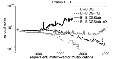
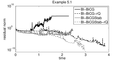
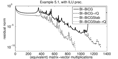
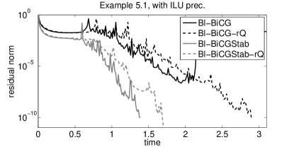
Figure 1 shows convergence plots for Example 1 without preconditioning (top row) and with a (right) no-fill ILU preconditioner (bottom row) obtained via the Matlab function ilu. The left plots show the relative Frobenius norm of the block residual as a function of the total number of matrix-vector multiplications (there are $2s$ of those per iteration). The right plots show the same residual norms, but now as a function of wall clock time. Figure 1 shows that both, Bl-BiCG as well as Bl-BiCGStab, can significantly improve when the QR factorizations are used, sometimes making iterations converge which otherwise would diverge. In the presence of preconditioning, where the preconditioned matrix is better conditioned and convergence is reached after a relatively small number of iterations, QR factorizations has a less pronounced effect, and standard Bl-BiCGStab actually now converges, too. Since computing a QR-factorization of a block of $s$ vectors of length $n$ requires an arithmetic cost of $\mathcal{O}(s^{2})$ vector operations, this cost is substantial unless $\rho$ is really small. From the plots in the right column of Figure 1 we indeed see that this additional cost is important and that more than outweighs the small gains in terms of the number of matrix-vector multiplications.

Table 2: Iteration counts #it, wall clock times and final residual norms $\|R\|$ for Bl-BiCG and its variant with QR-factorization of the block residual (top two rows), and their counterparts for Bl-BiCGStab (bottom two rows).

variants of Bl-BiCG (first two rows) and Bl-BiCGStab (last two rows), no precond.

Example 1

Example 2

Example 3

Example 4

Example 5

#it

time

$\|R\|$

#it

time

$\|R\|$

#it

time

$\|R\|$

#it

time

$\|R\|$

#it

time

$\|R\|$

500

2.28s

div.

500

43.83s

div.

500

44.99s

0.28

500

62.92s

1e-03

528

36.49s

3e-10

500

3.85s

1e-08

500

101.1s

div.

156

31.66s

2e-10

237

38.85s

3e-10

533

79.86s

3e-10

500

2.46s

0.093

500

45.15s

div.

111

9.73s

2e-10

175

20.66s

2e-10

1200

77.72s

2e-3

355

2.96s

1e-10

500

91.17s

div.

101

18.10s

2e-10

157

25.07s

2e-10

957

131.7s

3e-10

variants of Bl-BiCG (first two rows) and Bl-BiCGStab (last two rows), ILU precond.

Example 1

Example 2

Example 3

Example 4

#it

time

$\|R\|$

#it

time

$\|R\|$

#it

time

$\|R\|$

#it

time

$\|R\|$

500

7.72s

0.04

28

6.13s

2e-10

50

11.35s

3e-10

68

23.33s

2e-10

163

2.89s

1e-10

28

9.18s

8e-11

50

17.06s

3e-10

62

23.72s

3e-10

113

1.38s

3e-10

16

2.74s

4e-11

33

5.87s

6e-11

41

10.15s

2e-10

115

1.69s

3e-11

16

4.09s

3e-11

33

8.84s

5e-11

40

11.72s

7e-11

Table 2 summarizes the results for all our examples. For all four methods, it reports the number of matrix-vector multiplications and the time needed to reach the stopping criterion (reduction of the initial block residual by a factor of $10^{-10}$ or maximum of $500$ iterations reached in Examples 1-4, $1,\!200$ for Example 5). We also report the final relative norm of the block residual which was explicitly re-computed upon termination. If this final residual norm is larger than 1, we interpret this as divergence, noted as “div.” in the table. Smaller residual norms like $10^{-4}$ may be interpreted as an indicator of slow convergence, too slow to be competitive within our setting.

Table 2 confirms our conclusions from the discussion of Figure 1: QR-factorization improves numerical stability, and it has the potential to turn otherwise divergent iterations into convergent ones. Its (relative) additional cost is indicated by the value of $\rho$ from (8), and it is relatively small for Examples 1 and 4, whereas it is relatively high for the other examples where it thus does not pay off in the cases where the non-stabilized method is already convergent. The known convergence problems of BiCGStab for Example 2, see [30], carry over to both variants of the block method, and we may conclude that the non-convergence is not a matter of numerical stability but of BiCGStab and its block counterpart not being able to efficiently accommodate the relevant spectral properties of the respective matrix; see also the discussion in [30].

5.3 Comparison of all methods

Figure 2: Number of matrix-vector multiplications and time for all methods and all examples, no preconditioning.

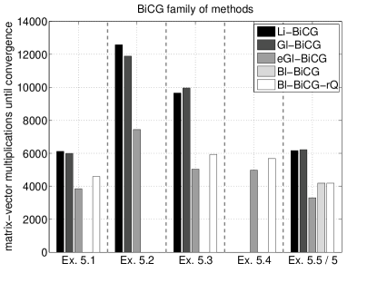
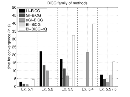
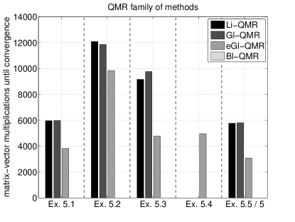
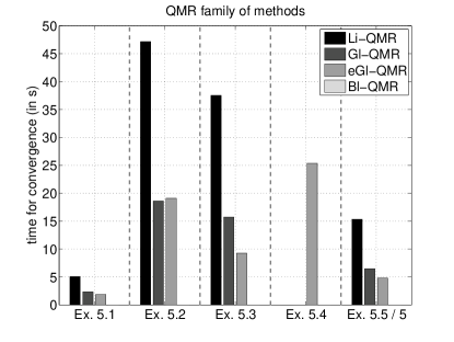
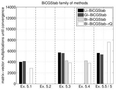
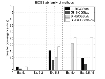
We proceed by comparing the number of matrix-vector multiplications and the wall clock times for all methods. Figure 2 does so for the case without preconditioning. We use bar plots to allow for an immediate visual comparison of the methods and we group our measurements by “families” of methods. Since Example 5 needs much more iterations than the other examples, we scaled the bar plots for this example by dividing by 5. A missing vertical bar indicates that the corresponding method either diverged or stagnated at a large residual norm. Instead of implementing a Bl-QMR method by ourselves we used a Matlab implementation by Freund and Malhotra which was publicly available at least until 2008 at the web site of Lucent technologies. This implementation is very cautious about possible ill-conditioning and (near) deflation, and for this reason it actually does all matrix-vector products one at a time, i.e. it does not use matrix-block vector products. As a result, this block QMR implementation can not be competitive with respect to timings, and for the unpreconditioned systems considered here we obtained premature break downs in all examples. The situation becomes slightly different in the preconditioned case, see below.

We can make the following observations: The loop-interchanged and the global methods require almost the same number of matrix-vector multiplications in all examples. Since the other arithmetic work is also comparable, this should result in similar wall clock times. This is, however, not what we see, the loop interchanged methods requiring substantially more time. We attribute this to the fact that the loop interchanged methods are the only ones were there is a non-negligible amount of interpreted Matlab code. “Plain” block methods suffer from non-convergence in a significant number of cases (8 out of 10). Using a QR-factorization of the residuals reduces the number of failures to 2. When they work, the block methods reduce the number of matrix-vector multiplications as compared to loop-interchanged or global methods by never more than a factor of 2. Because of the additional arithmetic cost, block methods never win in terms of wall clock time, and for larger values of $\rho$ (Examples 2, 3 and 5) they require more than twice the time than the corresponding global method across all “families”. The economic versions of the global methods always appear as the best within their respective “family”. They do not exhibit convergence problems, and they reduce the number of matrix-vector multiplications when compared with the global and loop interchanged methods. At the same time, their wall clock times are smallest. Overall, the economic global BiCG method appears to be the most efficient one, in tie with global BiCGStab for Example 1 and block BiCGStab for Example 4. Note that these are the examples with the smallest value for $\rho$.

Figure 3: Number of matrix-vector multiplications and time for all methods, Examples 1-4 with ILU preconditioning.

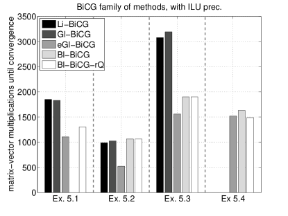
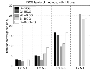
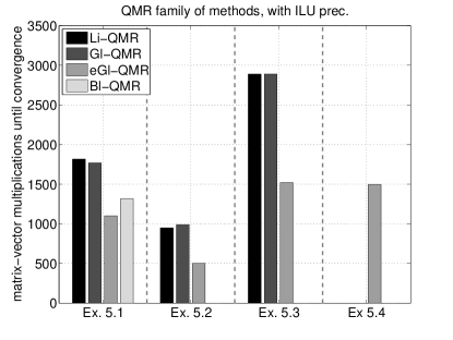
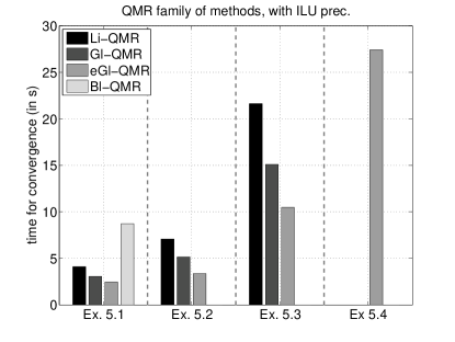
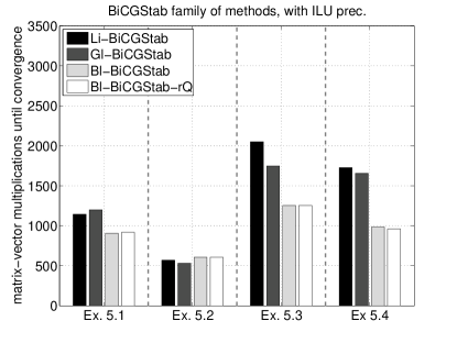
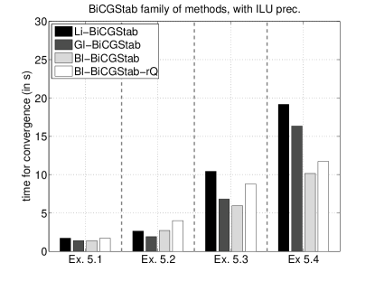
Figure 3 shows the results for Examples 1-4 where we now use ILU (right) preconditioning. More precisely, we used Matlab’s ilu do obtain a no-fill ILU in Examples 1-3 and an ILU with threshold and pivoting with a drop tolerance of $5\cdot 10^{-2}$ in Example 4. The number of matrix-vector multiplications and the wall clock times decrease for all methods as compared to the un-preconditioned case. Block QMR now converges for Example 1, but its wall-clock time is not competitive for the reasons explained earlier. The other block methods fail only once for BiCG, and never for BiCGStab. While the economic versions of the global methods still yield the best timings within their “family”, the block BiCGStab methods and global BiCGStab now perform better in terms of wall clock time for all four examples. The value of $\rho$ being particularly small for Example 4, this is the example where block BiCGStab gains most against loop interchanged or global BiCGStab.

Summarizing our findings we can conclude that one should use the block methods with particular care since there is a danger of non- convergence due to numerical instabilities. This can be somewhat attenuated by using the suggested QR-factorization of the block residuals. The additional arithmetic cost in the block methods should not be neglected, and—depending on $\rho$— there must be a substantial gain in matrix-vector multiplications in the block methods if this additional cost is to be outweighed. Global methods and loop interchanged methods require about the same amount of matrix-vector multiplications and additional arithmetic cost, so that they should require about the same time, too, if it were not for special effects in a Matlab implementation which mixes compiled and interpreted code. The economic versions of global BiCG and global QMR appear to perform well with respect to both, stability and efficiency. For better conditioned systems, e.g. when an efficient preconditioner is at hand, the block BiCGStab methods and global BiCGStab behave stably, and then their runtime is less than for the economic global methods.

References

- [1] J. I. Aliaga, D. L. Boley, R. W. Freund, V. Hernandez, A Lanczos-type method for multiple starting vectors, Math. Comp. 69 (2000) 1577–1601.
- [2] S. Birk, Deflated shifted block Krylov subspace methods for hermitian positive definite matrices, Ph.D. thesis, Bergische Universität Wuppertal, to appear (2015).
- [3] S. Birk, A. Frommer, A deflated conjugate gradient method for multiple right hand sides and multiple shifts, Numer. Algorithms 67 (2014) 507–529.
- [4] J. Cullum, T. Zhang, Two-sided Arnoldi and nonsymmetric Lanczos algorithms, SIAM J. Matrix Anal. Appl. 24 (2002) 303–319.
-
[5]
T. A. Davis, Y. Hu, The University of Florida Sparse Matrix
Collection 38 (1) (2011) 1:1–1:25.
URL http://doi.acm.org/10.1145/2049662.2049663 - [6] L. Del Debbio, L. Giusti, M. Lüscher, R. Petronzio, N. Tantalo, QCD with light Wilson quarks on fine lattices (I): First experiences and physics results arXiv 0702:056.
- [7] L. Del Debbio, L. Giusti, M. Lüscher, R. Petronzio, N. Tantalo, QCD with light Wilson quarks on fine lattices (II): DD-HMC simulations and data analysis arXiv 0702:082.
- [8] J. J. Dongarra, J. Ducroz, I. Duff, S. Hammarling, A set of level 3 Basic Linear Algebra Subprograms, ACM Trans. Math. Softw. 16 (1988) 1–17.
- [9] A. A. Dubrulle, Retooling the method of block conjugate gradients, Electron. Trans. Numer. Anal. 12 (2001) 216–233.
- [10] R. Fletcher, Conjugate gradient methods for indefinite systems, in: G. Watson (ed.), Proceedings of the Dundee Biennial Conference on Numerical Analysis, Springer-Verlag, New York, 1975.
- [11] R. W. Freund, M. Malhotra, A block-QMR algorithm for non-Hermitian linear systems with multiple right-hand sides, Linear Algebra Appl. 254 (1997) 119–157.
- [12] R. W. Freund, N. M. Nachtigal, QMR: A quasi-minimal residual method for non-hermitian linear systems, Numer. Math. 60 (1991) 315–339.
- [13] A. Frommer, K. Kahl, S. Krieg, B. Leder, M. Rottman, Adaptive aggregation based domain decomposition multigrid for the lattice Wilson Dirac operator, SIAM J. Sci. Comp. 36 (4) (2014) A1581–A11608.
[14]
M. Galgon, L. Krämer, J. Thies, A. Basermann, B. Lang, On the parallel
iterative solution of linear systems arising in the FEAST algorithm for
computing inner eigenvalues, Preprint BUW-IMACM 14/35, submitted (2014).
URL http://www.imacm.uni-wuppertal.de/fileadmin/imacm/preprints/2014/imacm_14_35.pdf - [15] C. Gu, Z. Yang, Global SCD algorithm for real positive definite linear systems with multiple right-hand sides, Appl. Math. Comput. 189 (2007) 59–67.
- [16] A. E. Guennouni, K. Jbilou, H. Sadok, A block version of BiCGSTAB for linear systems with multiple right-hand sides, Electron. Trans. Numer. Anal. 16 (2003) 129–142.
- [17] M. H. Gutknecht, Block Krylov space methods for linear systems with multiple right-hand sides: an introduction, in: A. H. Siddiqi, I. S. Duff, O. Christensen (eds.), Modern Mathematical Models, Methods and Algorithms for Real World Systems, Anamaya Publishers, New Delhi, India, 2007, pp. 420–447.
- [18] M. Heyouni, The global Hessenberg and global CMRH methods for linear systems with multiple right-hand sides, Numer. Algo. 26 (2001) 317–332.
- [19] D. Y. Hu, L. Reichel, Krylov subspace methods for the Sylvester equations, Linear Algebra Appl. 174 (1992) 283–314.
- [20] K. Jbilou, A. Messaoudi, H. Sadok, Global FOM and GMRES algorithms for matrix equation, Appl. Numer. Math 31 (1999) 49–63.
- [21] K. Jbilou, H. Sadok, A. Tinzefte, Oblique Projection Methods for Linear Systems With Multiple Right-hand Sides, Electron. Trans. Numer. Anal. 20 (2005) 119–138.
- [22] S. Karimi, F. Toutounian, The Block Least Squares Method for Solving Nonsymmetric Linear Systems with Multiple Right-hand Sides, Appl. Math. Comput. 177 (2006) 852–862.
- [23] D. P. O’Leary, The Block Conjugate Gradient Algorithm and Related Methods, Linear Algebra Appl. 29 (1980) 293–322.
- [24] E. Polizzi, Density-matrix-based algorithm for solving eigenvalue problems, Phys. Rev. B 79 (2009) 115112.
[25]
M. Röhrig-Zöllner, J. Thies, M. Kreutzer, A. Alvermann, A. Pieper,
A. Basermann, G. Hager, G. Wellein, H. Fehske, Increasing the performance of
the Jacobi-Davidson method by blocking, submitted.
URL http://elib.dlr.de/89980/ - [26] V. Simoncini, A stabilized QMR version of block BiCG, SIAM J. Matrix Anal. Appl. 18 (1997) 419–434.
- [27] V. Simoncini, E. Gallopoulos, An iterative method for nonsymmetric systems with multiple right-hand sides, SIAM J. Sci. Statist. Comput. 16 (1995) 917?933.
- [28] V. Simoncini, E. Gallopoulos, Convergence properties of block GMRES and matrix polynomials, Linear Algebra Appl. 247 (1996) 97–119.
- [29] V. Simoncini, E. Gallopoulos, A hybrid block GMRES method for nonsymmetric systems with multiple right-hand sides, J. Comput. Appl. Math. 66 (1996) 457–469.
- [30] G. L. Sleijpen, D. R. Fokkema, BICGSTAB(l) for linear equations involving unsymmetric matrices with complex spectrum, Electron. Trans. Numer. Anal. 1 (1993) 11–32.
- [31] H. Tadano, T. Sakurai, Y. Kuramashi, Block BiCGGR: A new block Krylov subspace method for computing high accuracy solutions, JSIAM Lett. 1 (2009) 44–47.
- [32] H. A. Van Der Vorst, Bi-CGSTAB: A fast and smoothly converging variant of Bi-CG for the solution of nonsymmetric linear systems, SIAM J. Sci. Stat. Comput. 13 (1992) 631–644.
- [33] B. Vital, Etude de quelques méthodes de résolution de problèmes linéaires de grande taille sur multiprocesseur, Ph.D. thesis, Univ. de Rennes I, Rennes (1990).
- [34] J. Zhang, H. Dai, J. Zhao, Generalized global conjugate gradient squared algorithm, Appl. Math. Comput. 216 (2010) 3694–3706.
- [35] J. Zhang, H. Dai, J. Zhao, A new family of global methods for linear systems with multiple right-hand sides, J. Comput. Appl. Math. 236 (2011) 1562–1575.