Large-scale clustering of Lyman- emission intensity from SDSS/BOSS
Abstract
We detect the large-scale structure of Ly emission in the Universe at redshifts by measuring the cross-correlation of Ly surface brightness with quasars in the Sloan Digital Sky Survey (SDSS/BOSS). We use nearly a million spectra targeting Luminous Red Galaxies (LRGs) at , after subtracting a best fit model galaxy spectrum from each one, as an estimate of the high-redshift Ly surface brightness. The quasar-Ly emission cross-correlation we detect has a shape consistent with a linear CDM model with . The predicted amplitude of this cross-correlation is proportional to the product of the mean Ly surface brightness, , the amplitude of mass density fluctuations, and the quasar and Ly emission bias factors. Using published cosmological observations to constrain the amplitude of mass fluctuations and the quasar bias factor, we infer the value of the product cm-2 Å-1 arcsec-2, where is the Ly emission linear bias factor. If the dominant sources of Ly emission we measure are star forming galaxies, we infer a total mean star formation rate density of yr-1 Mpc-3 at . For , this value is a factor of above previous estimates relying on individually detected Ly emitters, although it is consistent with the total star-formation density derived from dust-corrected, continuum UV surveys. Our observations therefore imply that of the Ly emission in the Universe at these redshifts is undetected in previous surveys of Ly emitters. Our detected Ly emission is also much greater, by at least an order of magnitude, than that measured from stacking analyses of faint halos surrounding previously detected Ly emitters, but we speculate that it arises from similar low surface brightness Ly halos surrounding all luminous star-forming galaxies. We also detect a redshift space anisotropy of the quasar-Ly emission cross-correlation, finding evidence at the level that it is radially elongated, contrary to the prediction for linear gravitational evolution, but consistent with distortions caused by radiative-transfer effects, as predicted by Zheng et al. (2011). Our measurements represent the first application of the intensity mapping technique to optical observations.
keywords:
Cosmology: observations1 Introduction
The Ly emission line of neutral hydrogen is a strong feature that has been used to detect galaxies at a wide range of redshifts (e.g., Hu & McMahon 1996, Keel et al. 1999, Fujita et al. 2003, Cowie et al. 2010). Another potentially useful technique is that of intensity mapping (e.g., Carilli 2011, Peterson & Suarez 2012, Pullen et al. 2014), which seeks to map the large-scale structure using one emission line or more (see e.g., Wyithe & Morales 2007, Visbal & Loeb 2010), without resolving individual sources (such as galaxies or gas clouds). By measuring this structure, one is sensitive to all clustered emission, without the observational biases which arise from source detection and luminosity measurement (such as detection limits, determination of backgrounds and finite aperture size). In this paper, we seek to perform the first cosmological measurement of intensity mapping in the Ly line, using a large dataset of spectra from the Sloan Digital Sky Survey III (SDSS-III, Eisenstein et al. 2011) Baryon Oscillation Spectroscopic Survey (BOSS, Dawson et al. 2013). We use spectra that were targeted at massive galaxies at . After subtracting best fit model galaxy spectra, we expect that any high redshift Ly emitters that are within the fiber aperture result in a residual flux, present also in sky fibers. Even if not detectable as individual sources, we can search for large-scale structure in this emission by determining its spatial cross-correlation function with the positions of BOSS quasars, which are tracers of structure with a known bias factor (e.g., White et al. 2012) at redshifts , where the Ly emission line is in the optical part of the spectrum.
Following the early prediction by Partridge & Peebles (1967) that galaxies should be detectable at high redshift from their Ly emission line, many surveys have been designed to detect individual galaxies as sources of Ly emission. These include narrow band imaging (e.g., Ouchi et al. 2003, Gronwall et al. 2007), serendipitous slit spectroscopy (e.g., Cassata et al. 2011) and integral field spectroscopy (e.g., van Bruekelen et al. 2005, Blanc et al. 2011). These techniques have resulted in the compilation of catalogs of several hundred to a few thousand Ly emitting galaxies from redshifts to the redshifts associated with the end of reionization. These samples have been used to show that Ly emitters of line luminosity found at have space densities of Mpc-3 (e.g., Gawiser et al. 2007, Cassata et al. 2015) and are therefore expected to be the progenitors of galaxies at redshift . The clustering of these galaxies has been measured on scales of up to 10 Mpc by Gauita et al. (2010) and Gawiser et al. (2007), who find that at redshifts they have a bias factor with respect to the underlying matter (in CDM models) of . Integrating the luminosity functions of Ly emitting galaxies, assuming a power-law extrapolation for the faint end slope, has revealed that the comoving volume emissivity of Ly photons declines significantly from to (Cassata et al. 2011, Gronwall et al. 2007, Ouchi et al. 2008). This behaviour can be compared to the opposite evolution in redshift of galaxies measured in optically thin parts of the rest-frame UV spectrum (or using the H line, e.g., Hayes et al. 2011). This comparison has been used to infer (e.g., by Hayes et al. 2011 and Cassata et al. 2011) that the escape fraction of Ly photons produced in star forming regions has significantly decreased from to .
Because Ly photons have a high cross-section for scattering off neutral hydrogen, extended Ly emission is expected to be common in many environments. For example, Ly radiation from star forming regions in galaxies should undergo hundreds or thousands of scatterings in gas in any circumgalactic medium before finally escaping or else being absorbed by dust. The existence of a general fluorescent emission from the intergalactic medium was also hypothesised by Hogan & Weymann (1987) and Gould & Weinberg (1996). Theoretical work applying line radiative transfer on gas distribution in cosmological hydrodynamic simulations has made predictions for Ly emission around galaxies and quasars (e.g., Cantalupo et al. 2005, Laursen et al. 2007, Kollmeier et al. 2010, Zheng et al. 2011a), as well as metal line emission (Bertone & Schaye 2012). These studies have resulted in predictions of extended Ly halos around galaxies with sizes of hundreds of kpc, with a strong dependence of their properties on environment that can lead to new effects on galaxy clustering (Zheng et al. 2011a).
Observational evidence for extended emission includes the discovery and characterization of the so-called Ly “blobs” (Steidel et al. 2000). Deep spectroscopic searches for diffuse Ly emission have been completed by Rauch et al. (2008), finding faint Ly emitting galaxies. Stacking of spectra of damped Ly absorbers in quasars has also produced measurements of residual Ly emission (Rahmani et al. 2010, Noterdaeme et al. 2014). Recently, Martin et al. (2014a,b) published the first results from the Cosmic Web Imager, an integral field spectrograph designed to map low surface brightness emission, detecting Ly emission from filamentary structures around a quasar as long as 250-400 proper kpc. Diffuse Ly halos around high redshift galaxies have been found to be ubiquitous by Steidel et al. (2011) and Matsuda et al. (2012). Momose et al. (2014) have assembled several samples of up to 3600 Ly emitters from Subaru narrowband imaging at a range of redshifts from to and, after controlling for atmospheric and instrumental artifacts, they detect diffuse extended Ly halos with exponential scale lengths of kpc from . The large scale studies in our paper are an alternative, complementary observational strategy to these earlier studies, which involve deep integrations over small fields of view.
All of these sources should be clustered on large scales and should contribute to the mean Ly emission intensity in the Universe. This mean emission is detectable if it cross-correlates as expected with other tracers of large-scale structure that we can observe at the same redshift. We shall use the quasars found by BOSS at to correlate with Ly emission in this work. This clustered Ly emission is extremely faint, but as we shall demonstrate it can be detected with BOSS thanks to the enormous number of spectra that are observed. While large-scale clustering measurements cannot easily allow separation of the signal into various sources, we may expect faint Ly emitting galaxies to dominate over quasars due to their much larger number density. If this is the case, then the mean Ly emission intensity clustered with quasars can be used as a measure of the global star formation rate (e.g., Cassata et al. 2011), times the mean (luminosity weighted) bias factor of the distribution of these galaxies. Our measurement of Ly emission will therefore be useful as a probe of star formation which takes into account all sources of Ly emission, reaching to arbitrarily faint luminosities and surface brightnesses from extended halos to faint galaxies.
The structure of this paper is as follows. Section 2 describes the data samples we use in our work, which include the galaxy and sky spectra from SDSS DR10, along with the quasar catalog from that data release. We present our measurement of quasar-Ly emission correlations in Section 3, including the evolution with redshift and clustering parallel and transverse to the line of sight. Section 4 describes our tests involving fitting and subtraction of emission lines. In Section 5, we convert our determination of the Ly surface brightness into a star formation rate density and compare to other measurements. In Section 6, we summarise our results and in Section 7 discuss them further. There are also three appendices to the paper, A-C; in these we measure stray light contamination, determine a large-scale surface brightness correction, and perform some sample tests of our results.
2 Data samples
This study makes use of data from the SDSS BOSS survey Data Release 10 (DR10, Ahn et al. 2014), including quasar position and redshift data, galaxy spectra and sky fiber spectra. The SDSS camera and telescope are described in Gunn et al. (1998) and Gunn et al. (2006), respectively. Full information on the SDSS/BOSS spectrographs can be found in Smee et al. (2013). The wavelength coverage of the spectrograph is from 3560 Å to 10400 Å the resolving power is for the range Å 4900 Å, and is kept above for the remainder of the wavelength range. The fibers have a diameter of 120 m, corresponding to arcsec. in angle. We restrict the redshift range of data we use in our analysis to , due to the spectrograph cutoff at low redshift and the limited number of observed quasars at high redshift.
2.1 Spectra
The 987482 galaxy spectra in our sample are of targeted LRGs which are within redshifts and . The redshift range of the original targets is not important to our study, as for each spectrum we make use only of the pixels for which the Ly emission line lies within the redshift range specified above ( ). In observed wavelength units this is 3647 Å to 5470 Å. We also make use of 146065 sky fiber spectra.
The main BOSS LRG program consists of two galaxy target samples (see Dawson et al. 2013), designated CMASS (for “constant mass”) and LOWZ (for “low-redshift”). The LOWZ galaxy sample is composed of massive red galaxies spanning the redshift range The CMASS galaxy sample is composed of massive galaxies spanning the redshift range . Both samples are color-selected to provide near-uniform sampling over the combined volume. The faintest galaxies are at for LOWZ and for CMASS. Colors and magnitudes for the galaxy selection cuts are corrected for Galactic extinction using Schlegel et al. (1998) dust maps. We do not differentiate between CMASS and LOWZ samples in our analysis.
The spectroscopic measurement pipeline for BOSS is described in detail in Bolton et al. (2012). The most important data products that are used in the present analysis are: (a) Wavelength-calibrated, sky-subtracted, flux-calibrated, and co-added object spectra, which have been rebinned onto a uniform baseline of (about 69 km s-1 pixel-1). (b) Statistical error-estimate vectors for each spectrum (expressed as inverse variance) incorporating contributions from photon noise, CCD read noise, and sky-subtraction error. (c) Mask vectors for each spectrum.
2.1.1 Data preparation
For each of the LRG spectra, we subtract the best fit model spectrum provided by the pipeline. This template model spectrum (see Bolton et al. 2012 for details) is computed using least-squares minimization comparison of each galaxy spectrum to a full range of galaxy templates. A range of redshifts is explored, with trial redshifts spaced every pixel. At each redshift the spectrum is fit with an error-weighted least-squares linear combination of redshifted template “eigenspectra” in combination with a low-order polynomial. The polynomial terms absorb Galactic extinction, intrinsic extinction, and residual spectrophotometric calibration errors (typically at the level) that are not fully spanned by the eigenspectra; there are three polynomial degrees of freedom for galaxies. The template basis sets are derived from restframe principal-component analyses (PCA) of training samples of galaxies, and have four degrees of freedom (eigenspectra).
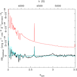
After subtraction of the best fittting template spectrum, we compute the average residual spectrum of all galaxies. This is displayed in Figure 1 where the horizontal axis is labelled in units of the redshift of the Ly line. Figure 1 also presents the mean sky spectrum and the sky-subtracted sky spectrum.
We can see that the residual surface brightness per unit wavelength (hereafter shortened to “surface brightness”- we use this term to refer to the quantity measured throughout the paper, which is most precisely the flux density per unit solid angle per unit wavelength) in the galaxy fibers is within for most of the redshift range. There are however significant excursions corresponding to features including the zero redshift Calcium H and K lines (at 3969 and 3934 Å) and a strong Mercury G line from streetlamps (at 4358 Å). In our analysis we subtract the mean residual surface brightness, from all spectra before cross-correlating them as we are only interested in the fluctuations in the Ly surface brightness. In order to reduce noise, we also mask two regions corresponding to large features in the residual surface brightness, 40 Å and 30 Å windows centered on wavelengths 3900 Å and 4357 Å respectively (corresponding to redshifts and 2.58).
Comparing the sky fiber and galaxy fiber residual spectra, we can see that there are differences at the level over much of the spectra. We attribute these to galaxy surface brightness that was not subtracted perfectly by the galaxy model. In our cross-correlation technique for measuring clustering in the Ly emission we necessarily subtract the mean surface brightness, therefore residual fluctuations seen in Figure 1 are not problematic except for the noise they contribute.
2.2 Quasars
We use quasars from the SDSS/BOSS DR10 catalogue (Ahn et al. 2014). The quasar target sample included both color-selected candidates and known quasars (Bovy et al. 2011; Kirkpatrick et al. 2011; Ross et al. 2012). The candidate quasar spectra were all visually inspected and redshift estimates computed using a principal component analysis (see Pâris et al. 2012 for the details of the procedure as applied to DR9 quasars). We select the 130812 quasars in the DR10 dataset that have redshifts in the range . Because the galaxy pixels cover this redshift range uniformly, the central redshift of our measurements is the mean redshift of these quasars, .
3 Quasar-Ly emission cross-correlation
Before computing the quasar-Ly emission cross-correlation, we first split the sample of galaxy spectra into 100 subsamples of approximately equal sky area based on contiguous groupings of plates. We then convert the galaxy spectrum pixels and the quasar angular positions and redshifts into comoving Cartesian coordinates using a flat cosmological model with matter density , consistent with the Planck, Ade (2014) results (cosmological constant density ). This fiducial model is used throughout the paper.
We compute the quasar-Ly emission surface brightness cross-correlation, , using a sum over all quasar-galaxy spectrum pixel pairs separated by within a certain bin:
| (1) |
where is the number of pixels in the bin centered on quasar-pixel distance , and is the residual surface brightness in the spectrum at pixel for the bin . Note here that we have a different list of pixels labeled as for each bin in the separation between a pixel and a quasar, which has Ly surface brightness . The residual flux at each pixel is obtained by subtracting the mean at each redshift, . We weight each pixel by , where is the pipeline estimate of the inverse variance of the flux at each pixel. We first present our results as a function of only the modulus of the quasar-pixel separation in comoving , in 20 bins logarithmically spaced between and . In Section 3.3 we will also examine redshift space anisotropies in the correlation function by considering bins in the parallel and perpendicular components of , using the same formulation.
When evaluating equation 1, a possible signficant systematic error is caused by stray light from the quasars themselves contaminating spectra of nearby galaxies. This occurs because the light from the various fibers is dispersed onto a single CCD, so that extraction of each spectrum along one dimension (Bolton et al. 2012) may include light from adjacent fibers of bright sources. We see strong evidence of this stray light from quasars in galaxy spectra when the quasar and galaxy spectra are four fibers apart or fewer, in the list of fibers as they are ordered in the CCD. The effect is discussed in detail in Appendix A. When the galaxy and quasar spectra in a pair are more than 4 fibers apart, we see no evidence for this contamination, and the results are statistically consistent with using only pairs of quasars and galaxies on different plates (see Appendix A). In order to safely eliminate this stray quasar light when computing the flux cross-correlation with equation 1, we therefore apply the constraint that the quasar and galaxy fibers must be at least six fibers apart.
There is also the possibility that some clustering in the plane of the sky is generated by effects (e.g., galactic obscuration) which modulate both Ly surface brightness and quasar target selection. Appendix B presents measurements of for quasar-pixel pairs which are close together on the sky (i.e., in the transverse separation) but widely separated along the line of sight. This measurement enables us to quantify how much clustering could be caused by effects such as Galactic obscuration and to compute a correction term to be subtracted from our fiducial clustering result. We also measure for pairs which are close in the line-of-sight separation but widely separated on the sky. This latter measurement constrains how much spurious clustering is caused by large-scale variations in the line-of-sight direction, for example redshift evolution in the efficiency of galaxy subtraction, or flux calibration errors with wavelength that may be associated with sky lines. We apply the corrections to from Appendix B to our analysis below and in the other sections of the paper. We discuss the small-scale anisotropy of in Section 3.3 below. For now we note that application of the correction factors described above changes the amplitude and shape of our measured by less than in all cases.
We perform the pairwise computation of equation 1 for each of our 100 subsamples, and then compute the mean and standard deviation of using a Jackknife estimator. The Jackknife estimator is also used to compute the covariance matrix of :
| (2) |
where is the cross-correlation in bin for Jackknife sample , is the cross-correlation for bin for the full dataset, and the number of Jackknife samples is .
3.1 Fiducial result
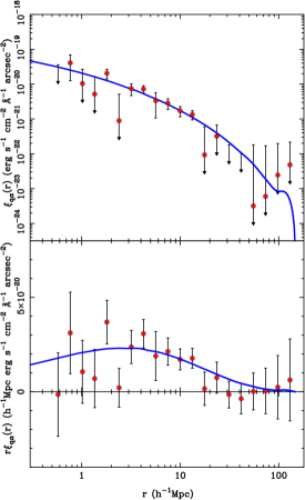
We show for our fiducial sample (which is the entire dataset over the redshift range ) in Figure 2. The mean Ly redshift of the galaxy pixels in this sample is and of the quasars . Because the galaxy pixel distribution is uniform in redshift, and because quasar-pixel pairs with small separations contribute most to the clustering signal, we adopt the effective mean redshift of our fiducial measurement to be . The cross-correlation function is in units of the surface brightness of Ly emission, and its amplitude is directly proportional to that surface brightness. The points reveal that there is significant measurable large-scale structure present in the Ly emission, on scales from to . Figure 2 also displays a linear CDM fit to the cross-correlation function, which is consistent with observational results on scales from . We turn to this fit in the next subsection.
3.2 Model fit
If the Ly emission clustering is due to a linearly biased version of the density field, then a model for the isotropically averaged quasar-Ly cross-correlation is as follows:
| (3) |
where is the mean surface brightness of Ly emission, and are the quasar and Ly emission linear bias factors, and is the linear CDM correlation function.
It is important to note that is the bias factor for Ly surface brightness fluctuations, and is different in definition from the usually quoted bias factor of Ly emitters, (e.g., as measured by Gawiser et al. 2007 and Guaita et al. 2010). The bias factor reflects the relation between the fluctuations in the number density of Ly emitters and that in the matter density ,
| (4) |
where and is the matter density field. The factor in Equation 3 relates fluctuations in the Ly surface brightness to matter fluctuations according to
| (5) |
In the absence of radiative transfer effect (Zheng et al. 2011a; see Section 6.4), the Ly surface brightness is proportional to the Ly luminosity density of the underlying star-forming galaxy population. The fluctuations of the latter can be characterized by the bias factor ,
| (6) |
and we have . As reflects weighting by luminosity rather than by number, it is likely to be significantly higher than , because higher luminosity emitters tend to be more strongly clustered. We will return to this topic in Section 5. Radiative transfer effect leads to a modification in the relation . In a simple model, we have with a positive number (see Section 6.4). Overall, we expect to be substantially higher than .
In Equation 3, is a constant enhancement to the correlation function on linear scales of the form that is caused by peculiar velocity redshift-space distortions (Kaiser 1987). We use the linear CDM transfer function of Lewis et al. (2000) to compute . In our computations we choose to vary the shape of the correlation function by changing , the matter density, in the context of the CDM model, keeping the other parameters which influence the shape (such as , and the baryon density ) fixed. Parameters have been reported for the best fit CDM model to the Planck Satellite data by Ade et al. 2014. We assume Planck values for and the spectral index but set . Note that we are merely using to parametrize the shape of the correlation function to see if it is consistent with other observations, and are not presenting our results for as properly marginalized measurements of that parameter.
The other free parameter is the amplitude, . We assume in all cases that the underlying amplitude of mass fluctuations , and therefore that , again consistent with Ade et al. 2014.
We fit our model to the data in Figure 2 by varying these two parameters. The value is given by
| (7) |
where the sum is over the bins, is the observed cross-correlation measured in bin , is the model prediction for bin , and is the covariance matrix computed using our 100 Jackknife samples in Equation 2.
The best fit values and one sigma error bars are as follows:
| (8) |
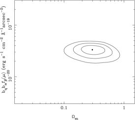
and . The shape parameter is consistent with the best fit value from the Planck satellite results (Ade et al. 2014, ). The 1, 2 and 3 confidence contours in these parameters considered together (i.e. =2.3, 6.17 and 11.8) are displayed along with the best fit values in Figure 3.
When carrying out our linear fit to the isotropically averaged correlation function we are neglecting non-linear effects and redshift measurement errors which are expected to suppress the correlation function on small scales (Davis and Peebles 1983). We are also not including in our model of Equation 3 the one-halo term (see e.g., Cooray and Sheth 2002) representing structure inside virialized halos, which would cause the correlation function to be increased at small scales. An estimate of the size of the redshift-space distortion effects is given below. There is some evidence for suppression of redshift-space distortions of the form that is expected from radiative transfer effects (Zheng et al., 2011a). The effect of the suppression terms in the cross-correlation function will be of opposite sign to the boost due to a one-halo term, so that the partial cancellation will further lower the impact of these effects. Because of these interactions, we leave more detailed nonlinear and halo modelling of the correlation function to future work.
3.3 Clustering transverse and parallel to line of sight
We also compute the quasar-Ly cross-correlation as a function of and , the quasar-pixel pair separation along and across the line of sight, shown in Figure 4, on a linear scale. We can see that the contours are relatively symmetric about the axis and somewhat stretched along the direction. Font-Ribera et al. (2013) found a redshift offset between quasars and the Ly forest of , due to the quasar catalogue redshifts being on average too small by this amount. This correlation resulted in the quasar-Ly forest cross-correlation being shifted upwards by this amount. The precision of the quasar-Ly emission cross-correlation in our paper is smaller, but visual inspection of Figure 4 reveals that the position of the centroid of the cross-correlation is consistent with a small upward shift of this magnitude ( at this redshift).
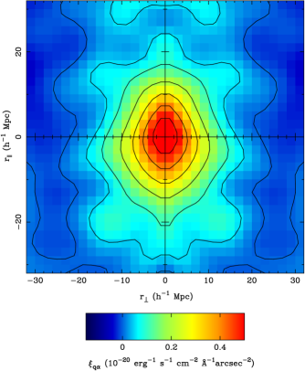
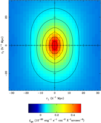
On the scales where the cross-correlation is easy to discern (), there is no sign of compression due to linear infall (Kaiser 1987). The redshift-space distortions should be less prominent compared to the Ly forest because of the expected higher bias for the Ly emission. In reality there appears to be stretching along the line of sight (we quantify this below), which might be due to a combination of quasar redshift errors, the intrinsic velocity dispersion of quasars in their host halos, or the intrinsic velocity dispersion of the sources of Ly emission.
Another source of apparent clustering anisotropy could be the radiative transfer effects predicted by Zheng et al. (2011a). It was shown by these authors, using cosmological radiation hydrodynamic simulations, that Ly radiative transfer has a strong environmental dependence which can cause the apparent spatial distribution of Ly emission to become anisotropic with respect to the line-of-sight direction. Density fluctuations along the line-of-sight direction are found to preferentially emit the Ly radiation in that direction in overdense regions, mainly because of the effect of peculiar velocity gradients on the Ly radiative transfer. This causes a suppression of the line-of-sight fluctuation, which can be modeled similarly to the Kaiser effect (also caused by the peculiar velocity gradient), even though the sign of the effect is opposite.
3.4 Fitting redshift-space distortions
In order to approximately quantify the level of distortion in Figure 4 and its statistical significance, we have investigated fitting a redshift-space distortion model to the data. To compute the model for , we first assume the linear CDM correlation function shape used in Equation 3 and then use a model for peculiar velocities to distort it in redshift space. Our pecular velocity model includes standard linear infall for large scale flows (Kaiser 1987) and a small scale random velocity dispersion (e.g., Davis and Peebles 1983).
The parameterization of the model for linear infall allows for stretching (outflow) as well as squashing (infall) along the line of sight. Although gravitational processeses are expected to result in infall, as mentioned above Zheng et al. (2011b) have shown that radiative transfer effects on the anisotropy of clustering can be approximately parametrized with the same model. We do this here, allowing a net linear outflow measured by the model to be interpreted as the radiative transfer effect.
The effects of coherent flows on the correlation function in linear theory were presented by Hamilton (1992). We use the formulation of Hawkins (2003), with modifications to make it appropriate for the case of cross-correlation functions. This modification involves the use of the two bias factors and from Equation 3 to compute redshift-space distortion factors and . The linearly distorted quasar-Ly emission cross-correlation function is then given by
| (9) |
where , and
| (10) |
| (11) |
| (12) |
with
| (13) |
| (14) |
Here is the linear CDM correlation function of equation (3).
We use these relations to create a model which we convolve with the distribution function of random pairwise motions, , to produce the final model :
| (15) |
The random velocity dispersion we use is an exponential model, thus the distribution function of velocities is
| (16) |
where is the pairwise velocity dispersion of quasars and Ly emission, which we assume to be independent of pair separation.
There is a strong degeneracy between and , but the bias factor for BOSS quasars is reasonably well measured. The first BOSS measurement, of , was made using the quasar autocorrelation function by White et al. (2012). Font-Ribera et al. (2013), find an even more precise value of from the cross-correlation of BOSS quasars with the Ly forest. Because of this we set , giving . The free parameters in our distortion model are therefore , and an amplitude parameter .

We set the parameter governing the shape in our model, , equal to the Planck value, . We compute for our model for a grid of values of varying , , and . We then compare our model to the observed from Figure 4, performing a fit to all points within . We again use jackknife error bars computed from 100 subsamples, but because of difficulties with noisy matrix inversion, we do not use the off-diagonal () terms when inverting the covariance matrix. We marginalize over the amplitude parameter , and show the confidence contours (for the two remaining degrees of freedom) in Figure 5.
We have allowed the parameter to be negative in our fit not because we believe that outflow of Ly emission is likely around quasars but, as mentioned above, because this allows quantifying the stretching along the line of sight seen in Figure 4 and its significance. Our best fit values with 1 error bars are and . From these values and by observing the contours in Figure 5, we infer a detection of anisotropies in the quasar-Ly emission correlation function that is opposite in sign to that expected from peculiar velocity flows due to gravitational evolution: our constraint on is from . We interpret this result as indicating that there are strong non-gravitational effects on the Ly emission causing the elongation of the cross-correlation contours along the line of sight extending to large separations; the good fit obtained with the redshift-space distortion model with negative needs to be understood in this case as a coincidence, since the model is not physically correct.
If we limit the fit to points with 20 , we find central values for and that are consistent with those for our fiducial fit, As might be expected, the error bars are larger, however, by a factor of for and for .
If we assume a Ly emission bias factor , corresponding to highly biased star forming galaxies, (see Section 5 for further discussion of this value), then at redshift . For the expected value of , we can use as a guide the results of Font-Ribera et al. (2013) who constrained at the 1 confidence level from the redshift-space quasar-Ly forest cross-correlation function. We can see from Figure 5 that although the measurement is consistent with Font-Ribera et al. , and considered jointly disagree at the level from our measurement.
We discuss further in Section 6 how our measurements can be interpreted as a detection of clustering anisotropies due to radiative transfer effects (Zheng et al. 2011b). In this case, elongation along the line of sight is expected, which can explain the effective measurement of a negative parameter.
The cross-correlation contours of the best fit model are plotted in Figure 4 (right panel), which also reveals stretching along the line-of-sight. The value for the fit is 610 measured from 400 bins, with 3 free parameters, a reduced of 1.5. The fit is therefore not good, and the discrepancy arises in large part in the central region, where the model has lower surface brightness than the observations. This result may be a sign that adding a one-halo term to the correlation function would provide a better fit, and should be addressed in future work with a larger data sample.
3.5 Large-scale tests
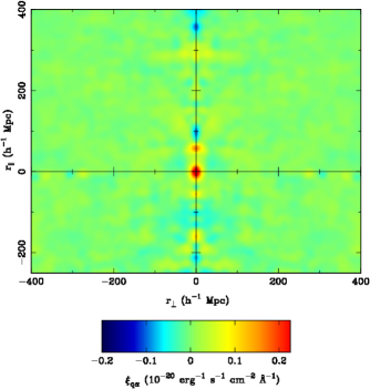
The cross-correlation across and along the line of sight over the whole spectrum offers a way to test whether the detected signal is reasonable. One can search for any significant cross-correlation signal if a different wavelength other than Ly is used, which would indicate either contributions from other emission lines, or that other effects are causing the cross-correlation signal meaasured. An equivalent approach is to extend the line-of-sight range of the cross-correlation to large distances. Figure 6, extends the contours shown in Figure 4 to much larger scales. The positive signal seen in Figure 4 is the most significant feature, centered at . This is a good indication that Ly emission is the dominant contribution to our signal. Signal from lines at longer (shorter) wavelengths than Ly would appear at positive (negative) values of .
The second most prominent feature, at , is significant at the level (the pixel at the center of the feature is 1.5 from the zero level, using the Jackknife error bars from Section 3.4), and so is consistent with noise. Strong lines that might be an issue, such as Lyman- and Carbon-IV, are very far away (at and +640 respectively) and so are not a concern. Si-III would appear at if it was present.
3.6 Evolution with redshift
The redshift coverage of our data sample () is sufficient that we can separate it into different bins in redshift and search for evolution. We do this for four different redshift bins where each bin contains one quarter of the quasar data. The bin boundaries and mean quasar redshifts of each bin are given in Table 1.
| (using ) | |||
|---|---|---|---|
| ( erg s-1 cm-2 Å-1 arcsec-2) | |||
| 2.20 | 2.0 | 2.29 | |
| 2.37 | 2.29 | 2.46 | |
| 2.59 | 2.46 | 2.75 | |
| 3.04 | 2.75 | 3.50 |
The quasar-Ly emission cross-correlation results are shown in the four panels of Figure 7. The global CDM model fit to the full sample averaged over all redshifts is indicated as the dash-dot line in every panel. Although the results for the redshift bins are relatively noisy, as expected, they are broadly similar to the global result in shape and amplitude and show no clear evidence for any redshift evolution.
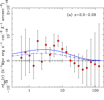
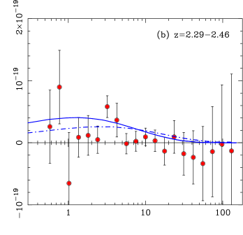
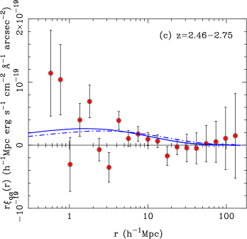
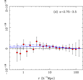
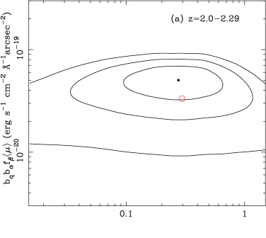
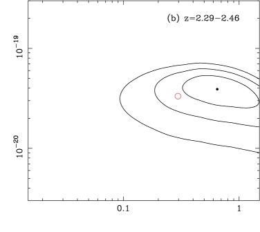
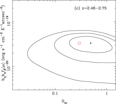
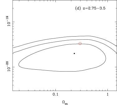
Figure 8 presents the best fit CDM shape and amplitude parameters from Section 3.2, along with confidence contours. The fitting was again performed using jackknife error bars. Figure 8 demonstrates that the fiducial model results all lie within the confidence contours for the different redshift bins.
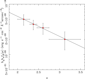
Assuming that the shape of the cross-correlation function remains fixed in comoving coordinates (as it would do if governed by linear biasing), we can search for changes in the amplitude of clustering and the mean Ly surface brightness as a function of redshift. We set (the CDM shape determined by the Planck results; Ade et al. 2014) and then determine the best fit amplitude parameters, , at each redshift bin. The result, shown in Figure 9, indicates a decreasing cross-correlation amplitude with redshift, although the errors are large and a horizontal line would not be an unreasonable fit “by eye”. To express this quantitively, we have carried out a fit to the function (), finding a slope parameter , meaning that the hint of redshift evolution is significant at the level only. The values for the fit parameters for the different redshift bins (which were used to plot Figure 8 are listed in Table 1.
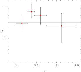
We have also looked at redshift evolution of the CDM shape governed by the parameter . Within the assumption of linear biasing, the shape should remain constant with redshift. The results are examined in Figure 10, where the results are indeed consistent with a constant , within the uncertainties. The Planck value () is also shown and is consistent with our results.
4 Emission lines
Given that the sources of the clustered Ly emission seen in Section 3 could be discrete objects such as star forming galaxies, we must investigate see if individual emission lines can be detected in our spectra and whether discrete detectable lines can account for the signal. The BOSS spectra have relatively short integrations on a small (2.5 m) telescope, and cannot be expected to compete in individual detections with other surveys such as that described in Cassata et al. (2011): we can only detect the most luminous objects. However, our cross-correlation technique enables us to find the mean total surface brightness, which includes all emission-line objects no matter how faint they may be. The difference between the cross-correlation signal with and without individually identified lines therefore enables us to discover what fraction of the Ly surface brightness lies below our line detection limit.
We note that our line detection procedure is less sophisticated than that in the BELLS survey (Brownstein et al. 2012), which used line detections of galaxies behind LRGs to find gravitational lenses. In particular, we are not seeking confirmed detections of objects (which requires multiple emission lines) and we do not deal with interlopers, except statistically.
4.1 Line fitting
For each LRG spectrum (see Section 2.1), we subtract the best fit galaxy spectrum model, as we do in our fiducial cross-correlation analysis. We then fit lines to this residual flux, centering our fitted line profile on the center of each spectrum pixel, one at a time. In this first stage, each spectrum pixel is therefore the center of a best fit line profile - we remove overlapping lines later. For each of a grid of values of amplitude and line width (between 0 and 20 Å) we compute the value of a positive Gaussian emission line profile , where the profile has the form and is the separation between the line center and the pixels we include in our fit. We use pixels in our fit that are in a 40 Å region centered on the line center, excluding masked regions as in Section 2.1.1. Once the best fitting values of and are found, we estimate the significance of each fitted line from the difference between the line fit and a flat interval with zero flux. After fitting to all the pixels we pass through the list and eliminate overlapping lines, removing the lower significance line when there is an overlap.
We find 5200 lines with a nominal significance of ( for the 2 degrees of freedom fitted), and lines with a nominal significance of () There are pixels in the search regions of the spectra. The detected lines are constrained to be at least 40 Å (37 pixels) apart, but for rare lines this should not change the random expectation. One would therefore expect to find approximately 370 and and lines respectively from positive noise fluctuations alone.
For the lines, the fact that we have detected fewer lines than even pure noise fluctuations predict is likely to be a sign that the fluctuations do not exactly obey a Gaussian noise model. An additional complication is that the noise estimate from the standard data pipeline which we have used has been shown to be underestimated by up to for the relevant wavelengths (Palanque-Delabrouille et al. 2013). The detection of more lines than randomly expected is likely to indicate that there are false detections arising from unsubtracted features in the galaxy spectra, sky lines we have not accounted for, and other systematics. There is also the possibility of interloping [OII] emission lines from lower redshift galaxies (see Noterdaeme et al. 2010, Menard et al. 2011). For our wavelength coverage of 3800-5500 Å, this interloper emission would arise from between and . Without a significant additional effort to remove false detections and interlopers, our dataset is not useful for computing the luminosity function of Ly lines. Instead, we turn to the statistical cross-correlation to test for the fraction of these lines which are really Ly emission lines in our redshift interval.
4.2 Cross-correlation
We subtract the flux in the lines detected in Section 4.1 from each LRG spectrum, and then recalculate the cross-correlation of quasars and Ly emission (Equation 1). The results for (again computing the error bars using a jackknife estimator and 100 subsamples) are shown in Figure 11, using our two thresholds on the significance of the removed lines, and . We can see that in each case, the clustering signal is still visible and the shape traces that of a CDM curve. This shows that most of the surface brightness of Ly emission is not accounted for by these lines. As expected, most of the lines are due to noise features. By subtracting these lines, however, we are also subtracting any possible real lines, and the change in the amplitude of is a measure of the fraction of surface brightness that is actually contributed by strong lines.
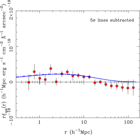
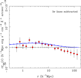
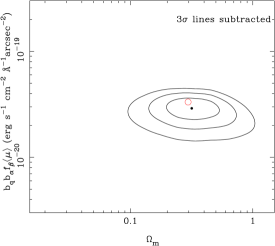
The shape and amplitude fitting parameters ( and ) for these two cases ( and lines subtracted) are shown in Figure 12. The shape parameter is very similar in the two cases and almost the same as in the fiducial case. The amplitude is lower, as would be expected for subtraction of some real lines, but the fiducial result (with no line subtraction) lies well within the 1 error contour of both of the panels in Figure 12, implying that the contribution to the cross-correlation from emission lines that are detected and removed is not statistically significant. Quantitatively, this can be seen by considering that we find the amplitude parameter for the case to be Å-1 arcsec-2, and for the case to be Å-1 arcsec-2. The amplitude parameter is therefore and lower than the fiducial case for the and line removal cases, but both of these are consistent with zero within the errors. The analysis is therefore consistent with our line fitting having found no true Ly emission lines at all.
In order to relate the significance levels to line luminosity, we have computed the luminosity from the surface brightness for each line (bearing in mind that our measurements are restricted to a 1 arcsec radius fiber aperture). We find that the median luminosity of the lines is and the lines have a median luminosity . We can compare these luminosities measured with some published values from Ly emitter surveys. The flux limit of the Guaita et al. (2010) data sample was (emission line flux) at z=2.1. This corresponds to a Ly luminosity of . For the Gawiser et al. (2007) sample at z=3.1, the line flux limit was , corresponding to a line luminosity of .
In our calculation above we have seen that at the 1 confidence level, of the Ly cross-correlation signal in our dataset could be due to lines with a median luminosity (in a 1 arcsec radius aperture) ergs-1. This is similar to the values of Gawiser et al. and Guaita et al. , although given our small aperture, the intrinsic luminosity of our fitted line emitters will be even higher. A small fraction of the value we are seeing could therefore be contributed by emitters similar to those in these two surveys. As noted above, the error bar on this fraction is large, and our result is consistent with zero contribution from such lines.

There are various possibilities for the nature of the major contributor to the Ly cross-correlation signal. The first is fainter lines than those seen in Ly emitter surveys. This is unlikely because is luminosity weighted, so low luminosity lines contribute much less to the signal than higher luminosity lines. The second is high luminosity, low surface brightness emission. This emission is much more difficult to detect, and cannot be seen by our line search algorithm, which is sensitive to high surface brightness, narrow lines. It is also unlikely to have been seen in previous surveys (we return to this in Section 6). This type of emission would also be highly biased, and so if present would contribute strongly to the measurement. We discuss the various possibilities in more detail in Section 6.
5 Star formation rate density
If the Ly surface brightness we are seeing is produced by star forming galaxies, we can convert the mean Ly surface brightness into a star formation rate density (SFRD) at the mean redshift of our observations. Traditionally (e.g., Gronwall et al. 2007) narrow band surveys have been used to detect Ly emitters, compute their luminosity function, and integrate it to compute a mean Ly luminosity density before converting it into a star formation rate, using a relationship such as:
| (17) |
(Cassata et al. 2011), where is the Ly luminosity. The conversion factor is based on a stellar population with a Salpeter IMF and with no correction for effects like dust and escape fraction, which is accurate to within a factor of a few for a range of population age, high mass cutoff of stars, and metallicity (Leitherer et al., 1999).
This method assumes that the surveys of Ly emitters are able to capture all the radiation from young stars. However, these surveys can only detect the high surface brightness portion of sources within a small angular aperture, and may be missing much of the Ly line intensity when it is scattered far out into the galaxy halo. In our case, the statistical cross-correlation technique we are using should not be affected by any threshold in Ly surface brightness. We should therefore be able to compute the total star formation rate density from our measurement. One large uncertainty is absorption due to dust, which is known to significantly affect UV continuum and line estimators of star formation.
Recall that our measurement is of the quantity , so to compute the Ly surface brightness we need to have independent knowledge of , and . For the quasar bias factor we use the value measured for BOSS quasars by Font-Ribera et al. (2013), .
We recall that the bias factor is related to a luminosity-weighted bias factor , from the definitions in Equations 5–6 ( in the absence of radiative transfer effect), and is different from the number weighted bias factor of Ly emitters, . To understand the difference in the values of the two bias factors, we start with the following simple model for the Ly emission.
If we assume that there are galaxies per dark matter halo of mass and that Ly emission comes from galaxies in halos above a mass limit , then the spatial bias can be computed as follows (e.g. Berlind & Weinberg, 2002):
| (18) |
where is the bias factor for halos of mass and is the halo mass function. For the luminosity weighted bias factor, we have
| (19) |
where is the average Ly luminosity in halos of mass .
Observationally, a value of results from an average of the values measured by Gawiser et al. (2007) and Guaita et al. (2010), who find at and at , respectively. Using Equation 18, we find that corresponds to . In the calculation, we assume one galaxy per halo (), which overestimates by only a small factor (see the Appendix of Zheng, Coil, & Zehavi 2007). The mass estimation is consistent with, e.g., the analysis of Gawiser et al. (2007).
To estimate the luminosity-weighted bias factor , we need to know the relation between luminosity and halo mass. Assuming that , for we obtain 2.38, 4.40, and 6.84 for the values and 3, respectively. The differences between and are therefore substantial, the latter being usually much larger. To proceed further, we need to consider the likely relation between and . The Ly luminosity is related to the star formation rate in galaxies. Along the star-forming sequence, the star formation rate is inferred to be approximately proportional to the stellar mass (e.g. Daddi et al., 2007; Pannella et al., 2009; Lee et al., 2011). We therefore first make use of the relationship between halo mass and stellar mass found with abundance matching by Moster et al. (2010). It is in the form of a softened broken power law, and at the low-mass-end (high-mass-end) slope of the – relation is () with a transition mass around . Using this relation in Equation 19 yields for . In fact, the result is insensitive to ( for ), given the steep – relation (so low-mass halos are weighted less). If we modify the high-mass-end slope to to approximately account for the luminosity contribution from satellite galaxies, we obtain .
There are various uncertainties involved in deriving with this simple model. First, the slope of the star formation rate versus the stellar mass relation for the star-forming galaxy sequence can be slightly different from unity. We find that a 10% deviation from unity in the above slope leads to a change in the value of . Second, we assume that the Ly luminosity is proportional to the star formation rate. The way these two quantities track each other may vary as a function of star formation rate if, for example, the escape fraction of Ly photons varies. Another possibility is that a large fraction of the Ly emission comes from previously undetected sources or low surface brightness halos around galaxies. These factors will change the – relation and therefore the derived value of . Even with the above uncertainties, it is likely that is around 3.
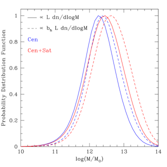
With the above model, we can compute the contribution to the Ly luminosity density from halos of different masses, which is simply proportional to the average Ly luminosity in halos of mass times the differential halo mass function . The solid blue curve in Figure 14 uses central galaxy Ly luminosity only, which peaks around . Including the contribution from the satellite galaxies shifts the peak slightly to a higher mass, around , as shown by the solid red curve. The curve gives the probability density of a random Ly photon to come from a halo of mass . The Ly emission detected through the cross-correlation technique probes the halo-bias-weighted luminosity density distribution. The dashed curves in Figure 14 show these probability distributions. With the satellite contribution included, the curve peaks around . Taking the full width at half maximum of the curve, the fiducial model implies that the signal in the cross-correlation should mainly come from Ly emission in halos of mass (1–20).
Finally, as mentioned in Section 3.2, is not the same as once the radiative transfer effect is taken into account. A simple model shows that with a positive number (see Section 6.4). The value of is not readily known without detailed radiative transfer modeling. Overall, we expect to be larger than 3. We choose to parameterize derived quantities in terms of .
An additional uncertain factor to consider is the modification to clustering caused by redshift-space distortions. This is embodied in the parameter. We have seen in Section 3.4 that measurements of anisotropies in clustering give a measurement of . This negative value of is of the form expected to be caused by radiative transfer effects on clustering (Zheng et al., 2011a) and is opposite in sign to the usual Kaiser (1987) peculiar velocity redshift-space distortions. Neverthless, this redshift-space distortion model was shown in Section 3.4 to give a reasonable fit to the data and one can use this to compute the factor as (from equation [10]). If we do this we find that the value of , which we take as a reasonable estimate of the reduction of the monopole term due the spreading the correlation along the line of sight. Even though gravitational evolution is not the physically correct model for interpreting our observations owing to the negative value we obtain for , a model with redshift-space distortion plus radiative transfer effect does seem to work reasonably well here (see Section 6.4).
We use this value and propagate the errors from the bias measurements and our measurement of (for fixed shape parametrized by ), to compute the mean Ly surface brightness at , finding
| (20) |
We convert this into a comoving Ly luminosity density using
| (21) |
where is the speed of light and . We find the value . We then use Equation 17 to convert this into a measurement of the star formation rate density . As mentioned before, the conversion depends on the assumption about the underlying stellar population. A younger population and lower metallicity would lead to a lower inferred SFR, which could be an important effect for interpreting our results. Keeping this possibility in mind, we proceed with the discussion by using the above result from the commonly adopted conversion factor.
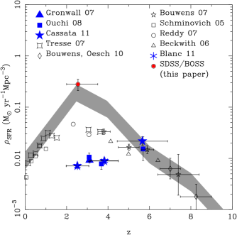
We plot this result in Figure 13 as the red point, for the chosen value of . We note that the true value for the parameter is not well determined, and that the datapoint should be scaled up and down by the factor . Our discussion above suggests that is likely to be larger than 3, so that it is more probable for to be scaled downwards than upwards. Figure 13 also shows various estimates of from Ly emitter surveys as well as UV continuum estimates of the star formation rate. We can see that our measurement is about 30 times higher (for ) than the Ly emitter based measurements of Gronwall et al. (2007), Ouchi et al. (2008) or Cassata et al. (2011). Note that these Ly emitter based measurements result from a direct integration over the observed Ly luminosity function without corrections for any possible dust effect.
A complication which adds substantial uncertainty is dust absorption, which may affect Ly and continuum radiation differently. One estimator of the level of dust extinction in the continuum is the rest-frame UV continuum slope, , which specifies how the flux density of a galaxy varies with wavelength (i.e., ) in the UV continuum region ( to ) of its spectrum. If an intrinsic -dust extinction relationship is assumed, (usually that measured empirically from galaxies by Meurer et al. 1999), one can use observations of for high redshift galaxies to infer a dust-corrected UV luminosity and then star formation rate. This has been done by several authors, including Bouwens et al. (2009,2010). In Figure 13 we show as a blue band the compilation of dust-corrected UV star formation densities from Bouwens et al. (2010) computed using this technique. According to Bouwens et al. (2010), the dust correction for a limiting luminosity of 0.3 is at redshift . Support for the validity of these corrections comes from the agreement of dust-corrected UV values with estimated from infrared observations (see the recent review by Madau & Dickinson 2014).
As for the effect of dust on the Ly radiation, Cassata et al. (2011) have speculated that it could be even stronger than proposed by Bouwens et al. (2010), as the Ly emitter inferred is less than 20% of the non-dust corrected UV continuum value (as can be seen in Figure 13). One reason which favors this interpretation is the fact that resonantly scattered radiation does have to cover a longer path length than continuum radiation before it leaves a galaxy so that it could be more vulnerable to dust extinction. On other hand, there is one well known mechanism (Neufeld 1991) which could preferentially enhance the escape of Ly radiation: in a clumpy medium of dusty clouds, continuum (UV) photons are absorbed as soon as their path crosses an optically thick dust cloud, whereas Ly photons can bounce off the cloud surfaces and find their way through the clouds to escape, leading to a lower extinction for Ly than for continuum photons if the intercloud medium is sufficiently devoid of dust. The anisotropic escape of Ly radiation (Zheng & Wallace, 2014) caused by, for example, a bipolar galactic wind, can also help make Ly photons follow the path of lower extinction optical depth to escape, while UV continuum photons are emitted isotropically and on average experience more extinction. From Figure 13, it appears that some mechanism of this sort is needed if we are to explain our results. We discuss these issues further in Section 6.
In conclusion, the rather surprising result seen in Figure 13 is that the fiducial value of the Ly surface brightness from our measurement is consistent with all Ly photons produced in stars at escaping from their host galaxies and being detected. The dust-corrected results of Bouwens et al. (2010) imply at , and from our measurement, . This means that is needed for our measurement not to imply detection of more Ly photons than are actually produced at more than the level. Our simple model for does satisfy this limit. We note that the intensity mapping technique we use in this paper will detect Ly photons which are scattered into our sightline from arbitrarily large distances from the emitting galaxy, and at arbitrarily low surface brightness. One can characterise our measurement as being consistent with a “total escape fraction” of Ly photons from star-forming galaxies of 100 %. This total escape fraction could be much higher from the “detected escape fraction” measured from traditional surveys of Ly emitters, which have surface brightness limitations. We also discuss this in more detail in Section 6.
6 Discussion
We can frame further discussion of our results in terms of the following questions:
-
1.
Can the observed Ly surface brightness be explained by known Ly emitters? We have seen in Section 5 that the simple answer appears to be no.
-
2.
Can the observed Ly surface brightness be explained by faint Ly emitters below the threshold of published surveys? Ouchi et al. (2008) have shown that changing the extrapolated luminosity function faint end slope from to changes the total integrated Ly luminosity density they infer by only . The answer to this question is therefore also no.
-
3.
Can the observed Ly surface brightness be explained by extended halos around the known Ly emitters? We show in Section 6.3.5 below that this is not the case, and that extended halos around known Ly emitters, while adding to the mean surface brightness, fall short of accounting for our results by an order of magnitude .
-
4.
Can the observed Ly surface brightness be explained by star-forming galaxies, when these are estimated based on the extinction-corrected UV continuum SFR density? We have seen in Section 5 that there appears to be just enough star formation per unit volume in the Universe at that if most of it led to escaped Ly emission, this could explain what we are seeing. We further discuss the implications of this below in Sections 6.2, 6.5 and 7.2.
-
5.
What is the contribution to our meaasurement of sources of Ly emission beyond star-forming galaxies? We address this in Section 6.3 below, showing that other contributions are likely to be very small.
6.1 Potential systematic errors in the measurement
Our measurement of Ly intensity clustering relies on statistical cross-correlation techniques applied to a large sample of spectra with relatively low signal to noise, all of which were targeted at bright foreground galaxies that we have removed in post-processing. There is therefore ample scope for small instrumental or other effects to influence the signal we measure. Bearing this in mind, we have carried out a range of tests, detailed in Appendices A-C, to make as certain as possible that the signal is real. Most importantly, these include tests of our methods for eliminating contaminating light from neighboring fibers, which does have a strong effect. We have also tested the effect of eliminating quasars clustered with the quasars we are using in our cross-correlation, and we have checked the dependence of the signal on the luminosity of the galaxy fiber target and on the quasar luminosity. For these latter tests, we have found no significant effect and therefore conclude that the signal is real, to the extent we have been able to ascertain.
There remains the possibility that some previously unknown effect, instrumental or otherwise, is responsible for the cross-correlation signal. This clustering signal would have to have a shape and amplitude consistent with CDM, yield a star formation rate density consistent with dust-corrected UV estimates, have clustering distortions of the form predicted by Ly radiative transfer effects, and pass all the tests mentioned above. This would constitute an unlucky coincidence; in particular, contamination by quasar light seems very unlikely once we have eliminated the effect of neighboring fibers in the BOSS camera and we have tested the absence of a dependence on the quasar measured flux. Galactic dust absorption or other systematics on the spectral continua also cannot induce the enhanced emission that is measured at the inferred Ly wavelength at the redshift of each observed quasar. However, the reader should bear in mind this possibility until future independent work is able to confirm our measurement.
We note that the effect of gravitational lensing on our results should be zero, even though we use spectra of bright galaxies, because our Ly measurements are of surface brightness, which is conserved under lensing. If on the other hand we were detecting Ly emitters in the fibers and obtaining their luminosity function, this would be subject to the well known magnification bias (e.g., Turner 1980). In our case, we are computing the cross-correlation function of the surface brightness measured from all fibers with quasars, and the magnification of Ly sources cannot change the amplitude of the cross-correlation. Dust associated with the foreground galaxies might reduce the Ly emission coming from higher redshift, but this could only further increase the inferred brightness of the Ly background.
6.2 Star-forming galaxies and the photon budget
We have found in Section 5 that our detected signal of cross-correlation of Ly surface brightness with quasars implies a brightness for the mean Ly photon background given by equation (20). This at the same time implies an emissivity of Ly radiation of . This emissivity can be reexpressed in terms of the rate at which Ly photons must have been emitted for each baryon in the universe at the mean redshift of our observation, . Using the comoving number density of baryons , and an expansion rate at of (using the parameters , , and , consistent with the most recent determinations from Planck in Ade et al. 2014), we find the following result:
| (22) |
The first, most simple assumption we make is that these photons are mostly originating from star formation in galaxies. The Ly photons created by recombinations in the HII regions produced around massive stars can then be scattered out to gaseous halos surrounding galaxies, from which they give rise to the background we detect in the quasar-Ly emission cross-correlation. As discussed in Section 5, this implies a very large star formation rate at . Equation (17) can also be recast in terms of the number of Ly photons emitted for each baryon that forms stars, :
| (23) |
Comparing to equation (22), we see that this implies that, for , about 10% of all the baryons in the universe would have to turn into stars if the star formation rate is maintained over the age of the universe at , years. The difficulty with this very high star formation rate is twofold: estimates of the total fraction of baryons in the form of stars at present are near 6% (Fukugita & Peebles 2014; Shapley 2011), and as described in the previous section, the total star formation rate at the redshift of our measurement can reach this value only for the maximum estimates of dust absorption, which would imply that while the UV continuum has to be absorbed by factors of , the Ly photons would have to emerge suffering little dust absorption.
A first possible solution to the problem of this extremely high inferred star formation rate is to modify the Initial Mass Function (IMF) of the stellar population that is assumed in deriving the Ly photons emitted per baryon in equation (22) from population synthesis models. If the slope of the IMF is flatter in the high mass range of , then stars above , which dominate the production of ionizing photons, increase their abundance compared to stars, which dominate the observed UV continuum. Most of the ionizing photons can be absorbed in HII regions, but most of the Ly photons produced by subsequent recombinations can escape, and their production rate can be increased compared to that inferred from the UV continuum observations. If the IMF stays flat down to lower masses, that can also greatly reduce the total star formation rate that is implied, as well as the stellar mass that is derived for the present universe which is measured from the old stellar population dominating the present luminosity of galaxies. If this flat IMF occurs particularly in massive galaxies with high metallicity, then the UV continuum observed at can be further reduced due to the suppression of blue horizontal branch stars, and the luminosity-weighted bias factor of the Ly emission can be further increased. A top-heavy IMF during the epoch when most stars were formed implies a large increase in the production of heavy elements, but this may be consistent with observations that show relatively high metallicities in the intracluster medium and in massive galaxies (Renzini & Andreon 2014).
For the rest of this section we assume a standard IMF with the ratio of Ly photons produced per baryon forming stars in Equation (22). We next enumerate additional sources that might contribute to this background other than star-forming galaxies, estimating if any of these contributions might be substantial. Finally, we discuss the effects of Ly radiative transfer on the quasar-Ly background cross-correlation we detect.
6.3 Other sources of Ly emission beyond star-forming galaxies
We shall discuss here four possible contributions to the quasar – Ly emission cross-correlation not arising from star-forming galaxies clustered around the quasars: (1) Scattering of the quasar Ly broad emission line by the Ly forest. (2) Fluorescence of the ionizing radiation from the quasar. (3) Scattering of the cosmic UV background by the Ly forest in the overdense IGM around quasars. (4) Fluorescence of the general cosmic ionizing background by the overdense IGM around quasars. (5) Ly cooling radiation from radiative dissipation of gas in halos that are correlated with quasars.
6.3.1 Scattering of the quasar Ly broad emission line
The average observed flux of our sample of BOSS quasars within the central of the Ly broad emission line is close to . In general, the mean fraction of light that is found to be absorbed by the Ly forest at is ( is the mean transmitted fraction; e.g., Faucher-Giguère et al. 2008). At a characteristic impact parameter of (inside which our cross-correlation signal is strongest), corresponding to an angular separation , the surface brightness of the scattered radiation should be , where is a dimensionless number that depends on the geometry of the scattering gas around the quasar and the shape of the Ly emission line, and has a value for a uniform gas density and a flat emission line profile. This yields a surface brightness , more than two orders of magnitude lower than our measured excess surface brightness at an impact parameter of from a quasar, as shown in Figure 2.
Scattered light from the quasar broad Ly emission line is therefore a negligible contribution to our detected Ly background. This is consistent with our test in Appendix C.3 showing no dependence of the cross-correlation amplitude on the quasar luminosity.
6.3.2 Fluorescence of the quasar ionizing radiation
An excess of Ly emission around the quasar may also arise from fluorescence of the ionizing radiation from the quasar. The ionizing radiation is absorbed in intergalactic absorption systems, and about half of the energy is reemitted as Ly photons when the recombinations that maintain ionization equilibrium take place. These Ly photons should be predominantly emitted from systems with column densities , for which the Lyman limit optical depth is of order unity.
The ratio of this fluorescent emission to the scattered Ly radiation from the quasar can be estimated as follows. The characteristic equivalent width of the Ly emission line of quasars is (see, e.g., the composite spectrum of BOSS quasars in Figure 16). Assuming a continuum slope bluewards of the Ly line for the average quasar, we find that the ratio of the number of ionizing photons to Ly photons emitted by a quasar is . Around two thirds of these absorptions of ionizing photons result in a Ly photon (the rest end up producing two-photon emission from the state of the hydrogen atom), whereas only of the Ly photons on the blue half of the quasar emission line are scattered in the Ly forest at . The ratio of the total number of fluorescent to scattered Ly photons from a quasar is therefore .
To estimate the ratio of the contribution to the excess Ly surface brightness near a quasar from the two processes, we also need to take into account the different pathlengths over which the photons are absorbed or scattered. Whereas Ly photons in the blue half of the quasar emission line will be scattered over a pathlength corresponding to the typical half-width of the Ly emission line, , the ionizing photons will be absorbed over the longer mean free path between Lyman limit absorbers at , which is (Prochaska et al. 2014). The surface brightness produced near the quasar is proportional to the total number of Ly photons produced divided by the pathlength over which they are emitted. Therefore, we conclude that the fluorescent emission from quasars should be times brighter in surface brightness than the scattered light from their Ly broad emission line.
Even this factor of 7, however, raises the estimated surface brightness contribution from fluorescence at an impact parameter to , which is still a factor of below our measured value at this impact parameter from Figure 2.
We note here that this Ly fluorescent emission from the quasar would not be of uniform intensity, but would predominantly arise from Lyman limit system absorbers in the quasar vicinity (see, e.g., the simulations in Kollmeier et al. 2010). This does not matter for our measurement, which is sensitive only to the mean surface brightness. In any case, our discussion suggests that the main difficulty for detecting this component of fluorescent emission caused by individual quasars probably lies in distinguishing it from the Ly emission scattered in gas halos surrounding star-forming galaxies that are clustered with the quasar, which is what we believe dominates the production of the Ly photons in our signal.
We also point out here that the quasar fluorescence contribution is affected by the anisotropy of the quasar emission and the time-delay between our observation of the quasar and that of the fluorescent light. Typically, if quasars are highly anisotropic and variable, the quasar emission in a direction away from the line of sight, or at years ago corresponding to the time when the quasar was illuminating an absorber at an impact parameter , would be systematically lower than the one we observe at present because of the flux-limited selection of quasar catalogues. These effects are likely to be important in any detailed modelling of the fluorescent emission due to the quasar.
6.3.3 Fluorescence of the cosmic ionizing background
Fluorescence from the mean cosmic ionizing background can also contribute to the quasar-Ly cross-correlation we measure. In this case, if we assume the intensity of ionizing photons from distant sources is uniform around the quasar, the effect on the cross-correlation would arise only from the overdensity of Lyman limit absorbers near the quasar, because a uniform Ly brightness does not contribute to our detected signal. We consider a value of the photoionization rate at of , which corresponds to a proper intensity per unit wavelength of the ionizing background of at the ionization edge (e.g., Faucher-Giguère et al. 2008). This ionizing background is being absorbed over a mean free path at (Prochaska et al. 2014). We assume that the ionizing background has a spectral slope in frequency (i.e., below ). Each ionizing photon produces a Ly photon with probability close to , so the intensity of the Ly background that is produced is
| (24) |
The factor arises from the ratio of the Ly to the Lyman limit wavelength (one factor for the energy of each photon, and one for the fact that the intensity is per unit of wavelength). This approximates as being independent of frequency, which is valid for optically thick absorbing systems (for optically thin systems, in the denominator needs to be replaced by , and the reality should be intermediate). Using , we obtain , at . When observed at the present time, the intensity of this Ly background is reduced to
| (25) |
This mean intensity now needs to be multiplied by the cross-correlation function of Lyman limit absorbers and quasars, to obtain the contribution to our measured cross-correlation. The value of the mass autocorrelation at impact parameter and is , which needs to be multiplied by the bias factor of quasars and the bias factor of Lyman limit absorbers. The bias factor for the BOSS quasars is known, , and that of the Lyman limit systems is unlikely to be larger than the value for DLAs, (Font-Ribera et al. 2012), implying that and is . This yields a value of the contribution to the quasar-Ly cross-correlation of , a factor of below our measured value from Figure 2.
We note that this estimate is consistent with a cruder calculation which uses the ionizing background observationally inferred by Fontanot et al. (2014) from the comoving space density of quasars and star forming galaxies. After exploring the likely parameter space of limiting magnitudes and escape fractions, Fontanot et al. (2014) find that a central value for the ionizing background comoving emissivity is about at . If the emissivity of the ionizing photons that are converted to Ly photons is at a similar level, with a conversion efficiency of 2/3, the fluorescent Ly emissivity is then . This is , times lower than the value inferred from our results.
We therefore conclude that fluorescence from the cosmic ionizing background also cannot be responsible for the large Ly brightness that we detect correlated with quasars.
6.3.4 Scattered Ly radiation from the radiation background
Just as scattering from the quasar by the Ly forest can in principle produce some contribution to this Ly light around quasars, one may think that the general ultraviolet continuum background from distant galaxies and quasars could also give rise to an excess of Ly photons near quasars because of the overdensity of the Ly forest that scatters this background radiation. However, this effect actually cancels out for our observation. High redshift galaxies that are behind the quasar should show the Ly forest absorption, reducing their ultraviolet flux, and this Ly absorption will be enhanced because of the overdensity surrounding the quasar. The background sources (which are of course too faint to be detected individually, but always contribute to our total background) are therefore fainter near quasars compared to any random fields. This is exactly compensated by the scattered Ly background from these same sources. For this reason, this contribution to the Ly background could only be detected if the individual sources behind the quasar were individually detected and subtracted out, before evaluating the Ly background intensity.
In addition to Ly photons scattered by the Ly forest, the background would also have a contribution from background photons reaching the Ly wavelength when passing near the quasar and being downscattered to Ly . This contribution is also very small, and is also nearly cancelled unless the population of ultraviolet sources creating the background evolves very fast over the redshift interval corresponding to the ratio of the Ly to the Ly wavelength. (note that the Ly forest does not contribute to this diffuse emission by intergalactic gas because Ly absorptions can only end in a 2-photon emission from the atomic state of hydrogen.)
6.3.5 Low surface brightness Ly halos around galaxies
We have described in Section 5 how Ly emission from galaxies could account for our measured result. Due to the magnitude of our signal, this Ly emission does not appear to originate in a straightforward way from Ly emitters seen in narrow band surveys at these redshift.
The Ly luminosity from observed Ly emitters is usually defined by pixels above certain surface brightness threshold or measured within an aperture (e.g., ; Ouchi et al. 2008). In any case, the surface brightness threshold is well above the sky noise and higher than the level associated with our measurement in this paper. An extended Ly emitting halo below sky noise level, resulting from Ly photons scattered by neutral gas in the circumgalactic and intergalactic media and clustered unresolved Ly sources, is predicted to exist around a star-forming galaxy based on radiative transfer modeling (Zheng et al., 2011b). Such diffuse Ly emitting halos are detected from stacking analysis (Steidel et al., 2011; Matsuda et al., 2012; Momose et al., 2014).
We use the stacked Ly surface brightness profiles and the fits to the diffuse Ly halos in Momose et al. (2014) to estimate the contribution of these halos to Ly emission in our detection. The luminosity inside the aperture of radius roughly corresponds to the Ly luminosity from the Ly emitter survey. We find that at both and , the diffuse Ly emission outside of is about one third of the luminosity inside the aperture. Therefore, the observed diffuse Ly halos, regardless of their origin, may only contribute an additional one third to the Ly emission from Ly emitter surveys.
This implies that our hypothesized extended emission from scattering halos that may account for our measurement would have to arise in many more galaxies than those detected in Ly -emission surveys.
6.3.6 Cooling radiation
Cooling radiation from gas in galactic halos can produce Ly emission. A rough estimate of the cooling radiation can be made if we assume that cooling and star formation reach a steady state on average in a galaxy (i.e., of gas cools per year to feed 1 yr-1 star formation). For gas initially at virial temperature dissipating the energy through cooling (as suggested by cosmological simulations; e.g., Fardal et al. 2001; Faucher-Giguère et al. 2010; Goerdt et al. 2010), we can estimate the corresponding cooling luminosity as follows:
Let us assume that a fraction of all baryons in the Universe fall into halos of virial temperature , and they dissipate all their energy by emitting Ly photons. Initially the baryons fall into the halo and are shock heated to temperature at a radius in the halo, where is the age of the Universe, and in the end they have to reach a radius by dissipating their energy through Ly emission, where is the half-radius of the galaxy.
The circular velocity is assumed to be flat, independent of radius. Then, the potential difference from to is . The energy to be dissipated per baryon is therefore . The relation between and the temperature is , where for the fully ionized mixture of hydrogen and helium from Big Bang nucleosynthesis. So, the total energy dissipated per baryon in the universe is
| (26) |
and the number of Ly photons emitted per baryon is
| (27) |
Using K and we get . With plausible values of , this could amount to nearly 15% of the emission we observed, and more if the bias of this Ly emission is high.
Cooling radiation is therefore the alternative source of Ly emission which comes closest to explaining our results, being plausibly less than an order of magnitude below our measurements. Cooling radiation could contribute in a substantial way to the observed Ly emission.
6.4 Radiative transfer effect
The above estimates show that the Ly emission relevant to our clustering measurements is likely to be dominated by contributions from star-forming galaxies. Regardless of the origin, as long as Ly photons are scattered by neutral hydrogen, we expect them to be affected by a radiative transfer effect. The quasar-Ly cross-correlation function we measure suggests that this effect is detected, shown as elongated contours along the line of sight on scales as large as 20. This feature cannot solely originate from the dispersion of the relative peculiar veclocity between quasars and galaxies (including redshift errors), but is consistent with the predicted main radiative effect on the clustering of Ly emitters in Zheng et al. (2011a).
The radiative transfer effect predicted in Zheng et al. (2011a) is a result of the anisotropic emission of scattered Ly photons from the anisotropic distribution of neutral gas density and velocity (hence anisotropic distribution of Ly scattering optical depth). In particular, Ly photons preferentially escape along the direction for which the neutral gas has the largest peculiar velocity gradient. Therefore, the Ly emission from less overdense regions along the line-of-sight direction would appear enhanced, suppresing the line-of-sight fluctuation. This dependece on the line-of-sight peculiar velocity gradient is analogous to that in the Kaiser effect but of opposite sign, leading to the elongated correlation contours. For all the possible origins of Ly emission discussed above, this radiative transfer effect should be at work as long as Ly photons interact with neutral gas on large scales.
Our measurement can be used to constrain the parameters relevant to the radiative transfer effect. Following the simple model presented in Zheng et al. (2011a), the real-space overdensity (the Ly surface brightness fluctuations here) can be related to the matter linear overdensty field and peculiar velocity field as
| (28) |
where is the Ly luminosity weighted bias of the underlying galaxy population and the line-of-sight peculiar velocity. The coefficient represents a combined effect of the dependence of the Ly radiative transfer (i.e., the Ly escape emission) on the density and the transverse peculiar velocity gradient, and specifies the impact of the line-of-sight peculiar velocity gradient (see Zheng et al. 2011a, in particular their Appendix A). Both coefficients are expected to be positive. In redshift space, we also need to add the Kaiser effect, and in terms of the Fourier component of the Ly surface brightness fluctuations, we have
| (29) |
The parameter (as constrained in § 3.4) is
| (30) |
The factor “1” comes from the Kaiser effect. The bias factor in Equation 3 is . With , we have (N.B. this is the coefficient defined in Wyithe & Dijkstra 2011). That is, the radiative transfer effect (indicated by a positive ) shows up or has been detected at a level of for the fiducial value of .
Overall, the quasar-Ly cross-correlation provides tentative evidence to a new clustering effect caused by Ly radiative transfer. A better measurement with a larger data set and a more detailed modeling will help understand this effect and use it to constrain the neutral gas distribution.
6.5 Escape fraction and detected fraction
Assuming now that our fiducial value of the star formation rate density is correctly inferred from the quasar-Ly cross-correlation, we conclude that it is consistent with the whole dust corrected star formation rate in Bouwens et al. (2010). At face value, this indicates that dust has little effect in reducing the Ly emission, i.e., almost 100% of the Ly photons produced from star formation escape. Clumpy dust clouds (Neufeld, 1991) and anisotropic Ly escape (Zheng & Wallace, 2014) may be possible mechanisms for explaining the high escape fraction of Ly photons, together with the much lower one for continuum UV photons.
We emphasize that the escape fraction is not the same as the fraction that is detected in Ly emitter surveys. The latter, the detected fraction, comes only from the central, high surface brightness part of the Ly emission from galaxies, and not from the extended Ly halos of low surface brightness (Zheng et al., 2011b; Steidel et al., 2011; Matsuda et al., 2012; Momose et al., 2014). The detected fraction for Ly emission at to 3, inferred from comparing the Ly luminosity density and Hα or Hβ luminosity density, is about 5% (e.g. Hayes et al., 2011; Ciardullo et al., 2014). This fraction is consistent with the ratio between the star formation rate density inferred from Ly emitters and that from quasar-Ly cross-correlation in this work (see the blue and red points in Figure 13).
7 Summary and Conclusions
7.1 Summary
We have carried out a cross-correlation analysis of residual light
in SDSS/BOSS galaxy spectra and SDSS/BOSS quasars at redshifts from
. We have used the Ly emission line (which
is at wavelengths Å at these
redshifts) to trace structure
in the cross-correlation. Our main findings are as follows:
(1) We measure large-scale structure in the quasar-Ly emission
cross-correlation at a mean redshift
at the 8 level.
The cross-correlation function shape is
consistent with the linear CDM correlation function.
(2) Looking at the clustering as a function of separation
across and along the line of sight we see evidence at the
level for distortions of
clustering of the form expected to be caused by radiative
transfer effects.
(3) We detect clustering independently in 4 subsamples
at different redshifts,
finding that the shape of the cross-correlation function is consistent
with the fiducial sample. The amplitude of the cross-correlation
increases by a factor of 3 between and , although this
detection of evolution is marginal, being consistent with no evolution
at the level.
(4) Although the spectra are too shallow to allow making a good
catalogue of emission lines, we are able to weakly constrain the
contribution of
emission lines to our signal statistically
by fitting lines, subtracting them and remeasuring the
quasar-Ly cross-correlation
function. We find that lines with luminosities (measured in our 1 arcsec
radius aperture) of erg s-1
may contribute of the quasar-Ly cross-correlation
amplitude at the relevant redshifts, but this contribution is still consistent
with zero.
(5) In one of our sample tests, we measure the cross-correlation
to be independent of quasar luminosity. This is evidence that the
large-scale clustering of Ly surface brightness
we measure arises mostly from Ly emission associated with star formation,
and not from any systematic error associated with the quasar light.
(6) We estimate the plausible contribution to the quasar-Ly surface brightness we measure from a variety of physical processes alternative
to star formation galaxies that follow the same large-scale structure as
quasars, such as fluorescence or scattering of the quasar emission or the
ionizing background, and we find these contributions to be almost all
negligible. Only cooling radiation may contribute in a substantial
fashion (perhaps at the level) to the Ly surface brightness.
(7) Using measurements of clustering from
SDSS/BOSS quasars, we convert the measured
amplitude of the cross-correlation function to the
product of mean
Ly sky brightness at and linear bias factor of Ly emission,
finding
erg s-1
cm-2 Å-1 arcsec-2.
Assuming that this Ly surface brightness is due to star
formation (see points (5) and (6) above), we convert our measured value to
the mean star formation rate density in the Universe at redshift ,
finding
.
This is consistent with dust-corrected UV continuum based estimates of
star formation, but more than an order of magnitude higher than previous
estimates of the SFRD from surveys of individual Ly emitters.
7.2 Implications
We conclude that the high intensity of the Ly background at that is derived from our measurement can only be reasonably produced by Ly -emitting galaxies that are clustered with quasars. If our measurement is confirmed, the consequences for our understanding of galaxy formation and evolution are dramatic. The Ly emission directly observed in Ly emitting galaxies so far at these redshifts contributes only to the mean star formation rate density. Extended halos that have been seen around these Ly -emitting galaxies detected in surveys can only contribute an additional to this value. We have detected ( range) times more Ly photons than the Ly emitter surveys (with the uncertainty due to the factor , and we have argued that most of these photons also arise from star formation. This amount of star formation represents most of the massive stars that are estimated to have formed in the universe and to have generated the present heavy elements.
To contribute to our measurement, these Ly photons cannot be absorbed by dust before escaping the galaxies. The question that remains then is how this Ly radiation could have been missed by previous observations. Putting forward and testing a detailed scenario is beyond the scope of this paper, but we speculate that all star forming galaxies at these redshifts, even if they do not have any detectable Ly emission line in their central parts, are surrounded by low surface brightness halos that nevertheless have a high total integrated Ly luminosity. These low surface brightness halos could allow the bulk of Ly photons to be below the detectable levels in narrow band Ly emitter surveys. As much of the star formation in the Universe at redshifts occurs in massive galaxies, the implication is that a large fraction of the Ly emission we detect is from giant low surface brightness halos around massive, bright, star-forming galaxies, which absorb most of their continuum photons to reradiate the energy in the infrared, and yet let their Ly photons escape.
7.3 The future
We note that the sky area covered by the million SDSS/BOSS (for our purposes randomly placed) fibers in the current study is square arc seconds. This is approximately of the entire sky area, showing that Ly intensity mapping holds an enormous promise as a probe of structure in the Universe. In addition to the quasar-Ly emission cross-correlation employed in the present paper, one can imagine carrying out Ly forest-Ly emission cross-correlations and Ly emission autocorrelation measurements. Correlations of Ly absorption and Ly emission, and vice-versa would avoid common mode systematics in the fluxing of spectrographs and may reduce the possibility of related error. As the Ly signal is distributed on large-scales, a way to efficiently carry out intensity mapping surveys (for example for baryonic acoustic oscillation experiments) may be to use integral field spectroscopy with relatively low angular ( 10 arcsec) resolution on a wide-field ( few deg.) telescope. If bright point sources could be masked such an instrument could in principle capture a dataset containing 5 orders of magnitude more information on large-scale clustering in the Universe than our present study.
Acknowledgements
RACC was supported by NSF Awards AST-1009781, AST-1109730, OCI-0749212, the Moore Foundation and by the Leverhulme Trust’s award of a Visiting Professorship at the University of Oxford. RACC would like to acknowledge the hospitality of the Astrophysics Subdepartment in Oxford where the intial stage of this work was carried out. RACC would also like to thank Matt McQuinn for useful discussions. JM is partially supported by Spanish grant AYA2012-33938. ZZ is partially supported by NSF grant AST-1208891 and NASA grant NNX14AC89G.
Funding for SDSS-III has been provided by the Alfred P. Sloan Foundation, the Participating Institutions, the National Science Foundation, and the U.S. Department of Energy Office of Science. The SDSS-III web site is http://www.sdss3.org/. SDSS-III is managed by the Astrophysical Research Consortium for the Participating Institutions of the SDSS-III Collaboration including the University of Arizona, the Brazilian Participation Group, Brookhaven National Laboratory, University of Cambridge, Carnegie Mellon University, University of Florida, the French Participation Group, the German Participation Group, Harvard University, the Instituto de Astrofisica de Canarias, the Michigan State/Notre Dame/JINA Participation Group, Johns Hopkins University, Lawrence Berkeley National Laboratory, Max Planck Institute for Astrophysics, Max Planck Institute for Extraterrestrial Physics, NewMexico State University, New York University, Ohio State University, Pennsylvania State University, University of Portsmouth, Princeton University, the Spanish Participation Group, University of Tokyo, University of Utah, Vanderbilt University, University of Virginia University of Washington, and Yale University.
References
- Ahn et al. (2014) Ahn, C., et al. 2014, ApJS, 211, 17
- Berlind & Weinberg (2002) Berlind A. A., & Weinberg D. H., 2002, ApJ, 575, 587
- Bertone & Schaye (2012) Bertone, S., & Schaye, J., 2012, MNRAS, 419, 780
- Béthermin et al. (2013) Béthermin, M., et al. 2013, A&A, 557, 66
- Blanc et al. (2011) Blanc, G.A., et al. , 2011, 736, 31
- Bolton et al. (2012) Bolton, A., et al. 2012, AJ, 144, 144
- Bovy et al. (2011) Bovy, J., et al. 2011, ApJ, 729, 141
- Bouwens et al. (2009) Bouwens, R. J., et al. 2009, ApJ, 705, 936
- Bouwens et al. (2010) Bouwens, R. J., et al. 2010, ApJ, 709, L133
- Brownstein et al. (2012) Brownstein, J. R., et al. 2012, ApJ, 744, 41
- Busca et al. (2013) Busca, N., G., et al. 2013, A& A A96, 1
- Cantalupo et al. (2005) Cantalupo, S., Porciani, C., Lilly, S., J., Miniati, F., 2005, ApJ, 628, 61
- Cassata et al. (2011) Cassata, P. et al. 2011, å, 525, 143
- Cassata et al. (2015) Cassata, P. et al. 2015, å, 573, 24
- Carilli et al. (2011) Carilli, C.L., 2011, ApJ, 730, L30
- Ciardullo et al. (2012) Ciardullo, R., Gronwall, C., Wolf, C., et al. 2012, ApJ, 744, 110
- Ciardullo et al. (2014) Ciardullo, R., Zeimann, G., Gronwall, C., et al. 2014, arXiv:1409.8304
- Chang, et al. (2010) Chang, T.-C., Pen, U.-L., Bandura, K. & Peterson J.B., 2010, Nature, 466, 463.
- Cooray & Sheth (2002) Cooray, A., & Sheth, R., 2002, Phys. Rep., 372, 1
- Cowie, Barger, & Hu (2010) Cowie, L.L., Barger, A.J., & Hu, E.M., 2010, ApJ, 711, 928
- Croft, Dalton, & Efstathiou (1999) Croft, R.A.C., Dalton, G.B.,& Efstathiou, G.P., 1999, MNRAS, 305, 547
- Daddi et al. (2007) Daddi, E., Dickinson, M., Morrison, G., et al. 2007, ApJ, 670, 156
- Davis & Peebles (1983) Davis, M., & Peebles, P.J.E., 1983, ApJ, 267, 465
- Dawson et al. (2013) Dawson, K.S., et al. , 2013, AJ, 145, 10
- Eisenstein et al. (2011) Eisenstein, D. J., et al. 2011, AJ, 142, 72
- Fardal et al. (2001) Fardal, M. A., Katz, N., Gardner, J. P., et al. 2001, ApJ, 562, 605
- Faucher-Giguère et al. (2010) Faucher-Giguère, C.-A., Kereš, D., Dijkstra, M., Hernquist, L., & Zaldarriaga, M. 2010, ApJ, 725, 633
- Font-Ribera et al. (2013) Font-Ribera, A., et al. 2013, JCAP, 05, 018
- Fontanot et al. (2014) Fontanot, F., Cristiani, S., Pfrommer, C., Cupani, G., & Vanzella, E. 2014, MNRAS, 438, 2097
- Fujita et al. (2003) Fujita, S.S. et al. , 2003, AJ, 125, 13
- Gauita et al. (2003) Gauita, L., et al. 2010, ApJ, 714, 255
- Gawiser et al. (2007) Gawiser, E., et al. 2007, ApJ, 671, 278
- Goerdt et al. (2010) Goerdt, T., Dekel, A., Sternberg, A., et al. 2010, MNRAS, 407, 613
- Gould & Weinberg (1996) Gould, A., & Weinberg, D.H., 1996, ApJ, 468, 462
- Gronwall et al. (2007) Gronwall, C., et al. , 2007, ApJ, 667, 79
- Guaita et al. (2010) Guaita, L. , Gawiser, E. , Padilla, N. , Francke, H. , Bond, N. A. , Gronwall, C. , Ciardullo, R. , Feldmeier, J. J. , Sinawa, S. , Blanc, G. A. and Virani, S., 2010, ApJ, 714, 255
- Gunn et al. (1998) Gunn, J.E., et al. 1998, AJ, 116, 3040
- Gunn et al. (2006) Gunn, J.E., et al. 2006, AJ, 131, 2332
- Hamilton (1992) Hamilton, A.J.S., 1992, ApJ, 385, L5
- Hawkins et al. (2003) Hawkins, E., et al. , 2003, MNRAS, 346, 78
- Hayashino et al. (2004) Hayashino, T., et al. 2004 AJ, 128, 2073
- Hayes et al. (2011) Hayes, M., Schaerer, D., Göran Östlin, Miguel Mas-Hesse, J., Atek, H., and Kunth, D., 2011, ApJ, 730, 13
- Hogan & Weymann (1987) Hogan, C.,J., & Weymann, R.J., 1987, MNRAS, 225, 1
- Hu & McMahon (1996) Hu, E.M. & McMahon, R.G., 1996, Nature, 6588, 231
- Kaiser (1987) Kaiser, N. 1987, MNRAS, 227, 1
- Keel et al. (1999) Keel, W.C., Cohen, S.H., Windhorst, R.A., and Waddington, I, 1999, AJ, 118, 2547
- Kirkpatrick et al. (2011) Kirkpatrick, J.A., Schlegel, D.J., Ross, N.P., Meyers, A.D., Hennawi,J.F., Sheldon, E.S., Schneider, D.P., Weaver, B.A., 2011, ApJ, 743, 125
- Kollmeier et al. (2010) Kollmeier, J. A., Zheng, Z., Davé, R., et al. 2010, ApJ, 708, 1048
- Laursen & Sommer-Larsen (2007) Laursen, P., and Sommer-Larsen, J., 2007, ApJ, 675, L69
- Lee et al. (2011) Lee, K.-S., et al. , 2011, ApJ, 733, 99
- Leitherer et al. (1999) Leitherer, C., Schaerer, D., Goldader, J. D., et al. 1999, ApJS, 123, 3
- Lewis, Challinor, & Lasenby (2000) Lewis, A., Challinor, A. & Lasenby, A., 2000, ApJ, 538, 473
- Matsuda et al. (2012) Matsuda, Y., Yamada, T., Hayashino, T., et al. 2012, MNRAS, 425, 878
- Menard, et al. (2011) Menard, B., et al., 2011, MNRAS, 417, 801
- Momose et al. (2014) Momose, R., Ouchi, M., Nakajima, K., et al. 2014, MNRAS, 442, 110
- Moster et al. (2010) Moster, B.P., Somerville, R.S., Maulbetsch, C., van den Bosch, F.C., Maccio, A. V., Naab, T. & Oser, L., 2010, ApJ, 710, 903
- Navarro, Frenk, & White (1997) Navarro, J. Frenk, C.S., & White, S.D.M., 1997, ApJ, 490, 493
- Neufeld (1991) Neufeld, D.A., 1991, ApJ, L85
- Noterdaeme (2010) Noterdaeme, P., et al., 2010, MNRAS, 403, 906
- Noterdaeme (2014) Noterdaeme, P., et al., 2014, å, 566, 24
- Ouchi et al. (2003) Ouchi, M., et al. 2003, ApJ, 582, 60
- Ouchi et al. (2008) Ouchi, M., et al. 2008, ApJS, 176, 301
- Palanque-Delabrouille et al. (2013) Palanque-Delabrouille et al. 2013, å, 559, A85
- Pannella et al. (2009) Pannella, M., Carilli, C. L., Daddi, E., et al. 2009, ApJ, 698, L116
- Pâris et al. (2012) Pâris, I. et al. 2012, å, 548, 66
- Partridge & Peebles (1967) Partridge, R.B. & Peebles, P.J.E., 1967, ApJ, 147, 868
- Peterson & Suarez (2012) Peterson, J.B., & Suarez, E., 2012, proceedings of Moriond Cosmology 2012, arXiv:1206.0143
- Prochaska et al. (2014) Prochaska, J., X., Madau, P., O’Meara, J., M., & Fumagalli, M., MNRAS, 438, 476
- Pullen, Doré, & Bock (2014) Pullen, A.R., Doré, O., & Bock, J., 2014, ApJ, 786, 111
- Rahmani et al. (2010) Rahmani, H., Srianand, R., Noterdaeme, P., & Petitjean, P. 2010, MNRAS, 409, L59
- Rauch et al. (2008) Rauch, M. , Haehnelt, M. , Bunker, A. , Becker, G. , Marleau, F. , Graham, J. , Cristiani, S. , Jarvis, M. , Lacey, C. , Morris, S. , Péroux, C. , Röttgering, H. and Theuns, T., 2008, ApJ, 681, 856
- Renzini & Andreon (2014) Renzini, A., & Andreon, S., 2014, MNRAS, 444, 3581
- Ross et al. (2012) Ross, N.P., et al. 2012, ApJS, 199, 3
- Ross et al. (2013) Ross, N.P., et al. 2013, ApJ, 773, 14
- Smee et al. (2013) Smee, S.A., et al. 2013, AJ,126, 32
- Steidel et al. (2000) Steidel, C. C. and Adelberger, K. L. and Shapley, A. E. and Pettini, M. and Dickinson, M. and Giavalisco, M., 2000, ApJ, 532, 170
- Steidel et al. (2011) Steidel, C. C., Bogosavljević, M., Shapley, A. E., Kollmeier, J. A., Reddy, N. A., Erb, D. K. and Pettini, M. ApJ, 2011, 736, 160
- Turner (1980) Turner, E.L, ApJ, 242, L135
- van Breukelen, Jarvis, & Venemans (2005) van Breukelen, C., Jarvis, M.J., & Venemans, B.P., 2005, MNRAS, 359, 895
- Visbal & Loeb (2010) Visbal, E. & Loeb, A., 2010, JCAP, 11, 016
- White et al. (2012) White, M., et al. 2012, MNRAS, 424, 933
- Wyithe & Dijkstra (2011) Wyithe, J. S. B., & Dijkstra, M. 2011, MNRAS, 415, 3929
- Wyithe & Morales (2007) Wyithe, J.S.B. & Morales, M.F., 2007, MNRAS, 379, 1647
- Zheng, Coil, & Zehavi (2007) Zheng Z., Coil A. L., Zehavi I., 2007, ApJ, 667, 760
- Zheng et al. (2011a) Zheng,Z., Cen, R., Trac, H., Miralda-Escudé, J., 2011a, ApJ, 726, 38
- Zheng et al. (2011b) Zheng, Z., Cen, R., Weinberg, D.H., Trac, H. & Miralda-Escudé,J. 2011b, ApJ, 739, 62
- Zheng & Wallace (2014) Zheng, Z., & Wallace, J. 2014, ApJ, 794, 116
Author affiliations
1 McWilliams Center for Cosmology, Dept. of Physics,
Carnegie Mellon University, Pittsburgh, PA 15213, USA
2 Astrophysics, University of Oxford,
Keble Road, Oxford OX1 3RH, UK
3 Institució Catalana de Recerca i Estudis Avançats,
Barcelona, Catalonia
4 Institut de Ciències del Cosmos, Universitat de
Barcelona/IEEC, Barcelona 08028, Catalonia
5 Department of Physics and Astronomy, University of Utah, 115 S 1400 E,
Salt Lake City, UT 84112, USA
6 Dept. of Astronomy and Astrophysics, The University of Chicago,
5640 South Ellis Avenue,
Chicago, IL 60615, USA
7 Department of Astronomy, Harvard University, 60 Garden St.,
Cambridge MA 02138, USA
8 APC, Université Paris Diderot-Paris 7, CNRS/IN2P3, CEA,
Observatoire de Paris, 10, rueA. Domon & L. Duquet, Paris, France
9 CEA, Centre de Saclay, IRFU, F-91191 Gif-sur-Yvette, France
10 Lawrence Berkeley National Laboratory, 1 Cyclotron Road, Berkeley,
CA 94720, USA
11 Department of Physics and Astronomy, University of California, Irvine, CA 92697, USA
12 Max-Planck-Institut für Astronomie, Königstuhl 17,
D69117 Heidelberg, Germany
13Department of Astronomy, University of Wisconsin, 475
North Charter Street, Madison, WI 53706, USA
14Department of Physics and Astronomy, University of Wyoming, Laramie,
WY 82071, USA
15 Departamento de Astronomia, Universidad de Chile, Casilla 36-D,
Santiago, Chile
16Université Paris 6 et CNRS, Institut d’Astrophysique de Paris,
98bis blvd. Arago, 75014 Paris, France
17Institute of Cosmology and Gravitation, University of Portsmouth,
Dennis Sciama building, Portsmouth P01 3FX, UK
18Department of Astronomy and Astrophysics, The Pennsylvania
State University, University Park, PA 16802, USA
19 Institute for Gravitation and the Cosmos, The Pennsylvania State
University, University Park, PA 16802, USA
20 Bldg 510 Brookhaven National Laboratory, Upton, NY 11973, USA
21 INAF, Osservatorio Astronomico di Trieste, Via G. B. Tiepolo 11,
34131 Trieste, Italy
22 INFN/National Institute for Nuclear Physics,
Via Valerio 2, I-34127 Trieste, Italy.
23 Department of Astronomy, Ohio State University,
140 West 18th Avenue, Columbus, OH 43210, USA
24 Apache Point Observatory, PO Box 59, Sunspot, NM 88349, USA
25 Department of Astronomy and Space Science, Sejong
University, Seoul, 143-747, Korea
Appendix A: Stray light contamination
As mentioned in Section 3 a potentially very important systematic is the contamination of the galaxy spectra by quasar light. This is particularly relevant for our cross-correlation measurement because we are searching for light from sources that are clustered with quasars, and light from the quasar itself could mimic this if not treated carefully. The issue arises because the 1000 fibers that orginate from the plate in the telescope focal plane are fed into (each red and blue) spectrograph and dispersed onto a single CCD. 1000 spectra are therefore extracted from a 4k4K chip and some light from neighbouring fibers can end up in CCD columns that are centered on other fibers.
A.1: Measured Quasar-Lyman- surface brightness correlation
We can test for this contaminating light by use of two facts about the observational setup. The fibers are arranged by fiber number (from 1-1000) on the CCD, so that for each spectrum we can measure light from a certain number of fibers away. Quasars and galaxies that we use in our cross-correlation will also often be measured on different plates, so that there is no possibility for this contamination. We can therefore also test our result by restricting the calculation of the quasar-Ly cross-correlation to pairs of quasars and galaxies lying on different plates.
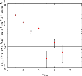
In the first test, we have computed the quasar-Ly cross-correlation of Equation 1 restricting ourselves to only quasar-galaxy spectrum pairs separated by specific values of , the difference in fiber number of the two spectra. Spectra with , are adjacent on the CCD, for example, and have the highest potential for cross-contamination of light. We reduce the quasar-Ly cross-correlation for each value of by averaging the results over a range from . Our conclusions about stray light contamination are not dependent on the range picked.
The results are shown in Figure 15, where we show against . In the plot the value of for our fiducial sample (Section 3.1), which uses all pairs with is shown as a horizontal line. We can see that for , the mean surface brightness inferred from the cross-correlation is over 20 times the fiducial value. It remains significantly higher for all . This is an indication that even when quasar and galaxy spectra are separated by 3 other spectra that light from the quasar is able to leak into the galaxy spectrum and contaminate it. Of course the particular region of the spectrum we are looking at (close to the Ly emission line at the redshift of the quasar) is the one in which the quasar is extremely bright, and one would not expect it to contaminate other parts of galaxy spectrum as much. Nevertheless, for our project, this is the important region of the spectrum, and we therefore must apply a cut on . Based on Figure 15, we have chosen that in our analysis.
A related test is to compute for quasars and galaxies that are on different plates (and therefore not dispersed at the same time onto the CCD). We show the results as a dashed line in Figure 15, which is indistinguishable from the results from our fiducial analysis. This is good evidence that our cut is sufficient to eliminate stray quasar light.
Yet another related test is to eliminate all galaxy fibers which have a quasar within a certain number of fibers. This is different from eliminating quasar-pixel pairs on a case-by-case basis because it will also eliminate any potential contamination which could come from quasars being clustered in space with other quasars. In the fiducial case, the contaminating quasars will have been eliminated directly, but those which are clustered with them could still contaminate the neigbouring galaxy spectra. One good reason to believe that this is not occuring to a detectable degree is that any contamination of this type would be a convolution of the redshift space autocorrelation function of quasars and the contaminating surface brightness from the quasar lya line, which is highly asymmetric and extremely elongated along the line of sight (see below). This does not appear to describe the measured signal (e.g., Figure 4).
Nevertheless, we have carried out the test, which eliminates % of the galaxy fibers from the data sample. We find an amplitude erg s-1 cm-2 Å-1 arcsec-2. and shape . These are consistent at about the 2 with the measurement from the fiducial sample. We note that the detection level of the signal is only about 3 overall, compared to for the fiducial measurement. This can be explained by the fact that eliminating all galaxies which have a quasar within 5 fibers will disproportionately affect the number of close quasar-pixel pairs. By directly counting, we find the number of quasar-pixel pairs with separations below 40 has fallen by a factor of 3.5 rather than the factor of 2 expected if pairs were drawn uniformly from all fiber separations.
We have also carried out another, similar test, which eliminates a smaller fraction of the dataset, but which should have the same effect. For this test we remove from our list of galaxy pixels all pixels which have more than 1 quasar within . In this way, we eliminate all potential cross-contamination from quasars clustered with the target quasars in the cross-correlation, but at a much reduced cost (doing this only eliminates 0.3 % of the galaxy spectrum pixels). After fitting the cross-correlation of this sample, we find an amplitude erg s-1 cm-2 Å-1 arcsec-2. and shape . This is consistent with the fiducial result within the error bars. It is slightly lower (by less than 1 ), which should not be surprising, as we are presumably preferentially removing some pixels in overdense regions. Overall these two test results are a good sign that significant cross-contamination from quasars clustered with the target quasar is not ocurring.

A.2 Modelling the stray light contamination
If the excess surface brightness seen above in galaxy spectra which are close on the CCD to quasar spectra is indeed due to cross-talk from quasar light, we would expect the contamination to have a quasar-like spectrum. To examine this, we first make a stacked spectrum of the DR10 quasar sample, by averaging all the spectra together in the quasar rest frame with unit weight. This is shown in Figure 16. We can see from that figure that the quasar Ly line is extremely broad, with a FWHM of Å in the rest frame. There is also the noticeable emission feature due to NV on the red wing of the line.
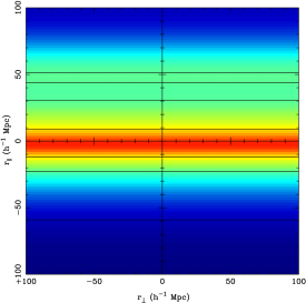
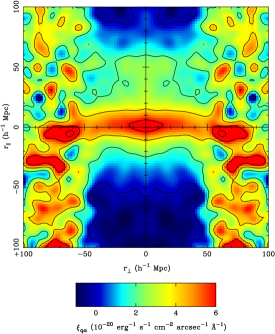
We next take this stacked spectrum, and convert the wavelength units into comoving at , the mean redshift of our measurements. If the quasar light is truly a contaminant, we expect the strength of the contamination to depend on the difference between fiber numbers (, as defined above) and not on the actual physical separation between quasar and pixel across the line of sight (). Plotting the quasar-Ly cross-correlation for particular values as a function of is therefore a useful check that light contamination is occuring as we believe. The prediction for the contamination, taken directly from the quasar spectrum is shown in the top panel of Figure 17. In that Figure we have scaled the overall amplitude by a factor of (see below). We can see that the large width of the Ly line, and its asymmetry due to the NV feature are both apparent.
The data with the strongest contamination should be from galaxy pixel-quasar pairs which are 1 fiber apart (=1). We therefore plot the quasar-Ly correlation for just those pixel-quasar pairs in the bottom panel of Figure 17. It is immediately apparent that there is a stripe across the middle of the plot corresponding to the contaminating quasar Ly emission line. The contamination is clearly asymmetric, extending further to positive values of than negative, and overall is visually consistent with the prediction based on the stacked quasar spectrum (top panel of Figure 17). Because the quasar-pixel pairs that are exactly 1 fiber apart only comprise a very small fraction of the data, we expect there to be lots of noise in the plot, particularly for large values of . This latter is because close pairs of quasars and galaxies on the sky are more likely to be close in . There is neverthless enough range that we can examine by eye whether the contamination depends on , with the answer appearing to be no. We examine this more quantitively below.

When comparing the top and bottom panels of Figure 17 we note that the amplitude of the stacked quasar spectrum is scaled by a factor of , which is the level required to match the observations in a fit (see below). This means that 0.2 % of the quasar light is scattered into neighboring spectra (i.e. spectra with ).
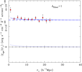
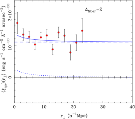
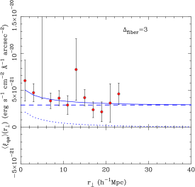
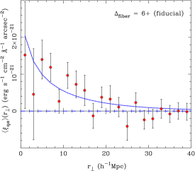
If there is a signal that is actually coming from quasar-Ly emission correlations in the Universe, one would expect that to be superimposed on top of any contamination from stray light. We have therefore carried out a simple joint fit of with a sum of the fiducial theoretical model from Figure 4 (right panel) scaled by an amplitude factor and the stacked quasar contamination scaled by a factor . The fit is therefore as follows:
| (31) |
where (multiplied by ) is shown in Figure 16 (top panel). We separate the observational results by and then carrying out a fit of the form given by Equation 31 to determine the best amplitude parameters and as well as the confidence limits on those parameters. We carry out the fit for quasar-pixel pair separations , although our conclusions are insensitive to this value.
The results are plotted in Figure 18. For the dataset, we find a total for the best fit of 1526 for 988 datapoints, which shows that the light contamination which dominates the fit is fairly well modelled by the quasar stack. It is perhaps not surprising the fit to the contamination is not perfect, as the contamination model is extremely simple. We have plotted the 1,2 and 3 confidence contours on the parameters and in Figure 18. The central value of is . The 1 confidence interval on is consistent with unity, and also with zero. The results from are therefore consistent with the sum of significant contamination from quasar light and a quasar-Ly correlation at the level predicted by the CDM model fit to the fiducial dataset.
We have carried out the same fitting to datasets with different restricted values of in the other panels of Figure 18. We can see that for cases with there is a significant detection of a contamination contribution. The value of is lower for than for at the factor of level. In all cases the measurements are also consistent with an additional quasar-Ly correlation at the level of . For and , the contamination is not detectable.
The results of the fitting shown in Figure 18 are a good sign that the signal and contamination are behaving in a particular way which can be accounted for by excising pairs of pixels from close fibers. It is useful however to examine the results for individual datapoints in more detail. Of particular interest is the measured quasar-Ly surface brightness as a function of . As mentioned above, we expect contamination at the CCD level for a given fiber separation to be independent of . We have taken the measured values for different datasets limited by and averaged them between .We plot this average, as a function of in Figure 19. In each panel we also plot a dashed horizonal line showing a level of contamination that is independent of , a dotted line showing the level of the signal from quasar-Ly clustering (we plot computed from the model shown in Figure4, right panel), and a solid line which is the sum of the two.
We can see that in the panel there is the strong contamination signal which is consistent with being independent of . The small relative contribution of the actual signal makes little difference in this panel. In the and panels the level of contamination is lower (note that the y-axes are different in the different panels), but it still dominates over the expected signal, with again no sign of a dependence on . For the fiducial panel (bottom right), we can see that the measured does have significant dependence on , and this has a similar form and amplitude to the best fit model to the data in Section 3.2. There is no sign of a contaminating (independent of ) component to this measurement.
Having carried out these tests on contamination from the Ly emission line from nearby quasars, it is pretty clear that the signal we are seeing in our fiducial dataset cannot be caused by straightforward scattered light coming from nearby fibers. There remains the possibility however that there is an additional contaminating component from some other mechanism that has a dependence on . This is difficult to imagine, but one can construct tests for this based on other spectral features than the Ly line. In the next two subsections we do this, first centered on the quasar CIV emission line and then using stars and the H line.
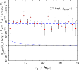
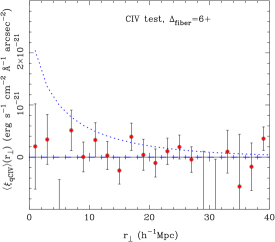
A.3 Tests with CIV
As a test of scattered light contamination, we carry out a different correlation between galaxy spectrum pixels and quasar positions. The only difference from our standard analysis (Section 3) is that we compute the cross-correlation at the wavelength of CIV at the redshift of the quasar. We use a rest wavelength of 1550 Å for CIV (close to the center of CIV doublet). If our interpretation of the contamination from nearby quasars from the previous subsection is correct, we would expect to see strong contamination from the CIV line for low and then no signal for large (because there should be no strong intergalactic CIV line emission).
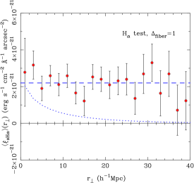
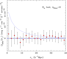
As with Figure 19, we plot , in Figure 20. We show results for and for . In the case of there is strong contamination from the quasar, which does not depend on . The amplitude of the contamination is approximately three times smaller than that from Ly , which is the ratio one would expect from the relative strengths of the two lines in Figure 16. For the we see that there is no evidence for contamination, and, although the error bars are relatively large, there is no sign of any signal. We have plotted the fiducial model on both panels with a dotted line. That the contamination behaves the same way as the Ly results in the previous subsection but that there is no signal is further evidence for the reality of the measurement.
A.4 Tests with stars
A further test of stray light contamination which we can carry out is to cross-correlate the positions of stars with the galaxy pixels. We use all stars in the SDSS DR10 catalog (Ahn et al. 2014), which is 171612 objects in total. In this case we choose the H line, with rest wavelength 6562.8 Å and cross-correlate star positions with galaxy pixels centered on this wavelength. We measure the resulting star-H cross-correlation, is for two values of , 1 and . In this test, all the stars are obviously at the same rest wavelength, which effectively means that in this measurement we are stacking galaxy spectra together. This test is therefore likely to be more sensitive to the CIV test to residual artifacts in photocalibration of the spectrometer (see e.g. Figure 4 of Busca et al. 2013). Nevertheless it is useful to see whether any contamination has an dependence.
We plot the results for in Figure 21, where we can see that there is again a sign of stellar light contamination when and that this contamination appears to be independent of . For , the measurement is consistent with zero, again a sign that the cut in removes scattered light contamination.
The results from the tests in Appendix A therefore suggest that although light contamination from quasars can be readily seen in the data, it can be eliminated to a high degree by excluding close pairs of fibers. When this is done, the resulting measured quasar-Ly surface brightness correlation seems to be real. If instead it is produced by some as yet unknown systematic this effect would have to reproduce the and dependence expected from a cosmological signal, be measurable only in the Ly wavelength range and not around other emission lines, and be independent of the position of the spectra on the detector.
Having searched for and as far as we can tell eliminated the effects of strong light contamination, we now turn to other potential systematic effects in the next 2 appendices.
Appendix B: Large-scale surface brightness correction
A potential systematic error on our measurement is any obscuration (such as that produced by Galactic dust) that may affect both quasar selection and Ly surface brightness, thus producing a spurious cross-correlation between the two on the plane of the sky. One can correct for such a cross-correlation by searching for an signal which is non-zero for large values of , where no physical (3D) correlation would be expected. This correlation which will be a function of only (in the parallel line-of-sight approximation) can then be subtracted from the signal. We have done this, computing the surface brightness correction given by
| (32) |
where and and is the qso-Ly emission cross-correlation. The value of is shown in the bottom panel of figure 22. We can see that there is no coherent structure, as becomes both positive and negative as varies. We have also plotted the best fit linear CDM model (as a function of ) for the qso-Ly cross-correlation (from Section 3.2), and we can see that this dominates over the correction on small scales , as we would hope.
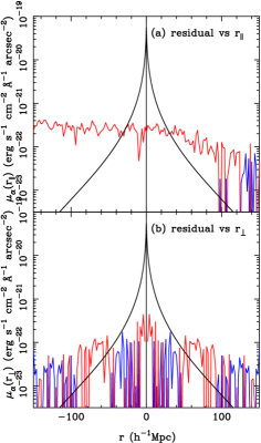
There is also another analogous correction, but one that applies in the orthogonal direction. Any systematic effect which affects the Ly emission in the line-of-sight direction (including redshift evolution in the Ly surface brightness), and which is correlated with evolution in the quasar population with redshift (or at least evolution in the efficiency of quasar selection with redshift) could produce a spurious qso-Ly emission cross-correlation. We compute how varies as a function of for large values where there should be minimal physical clustering. In this case the the surface brightness correction is given by
| (33) |
where we use the same values of and as in Equation 32. The results for are shown in the top panel of Figure 22. We can see that in this case there is a significant trend in the surface brightness correction with gradually decreasing from positive values of erg s-1 cm-2 Å-1 arcsec-2 for to erg s-1 cm-2 Å-1 arcsec-2. for . As with the previous () correction, the CDM model dominates on scales , where most of the clustering signal is located.
In our analyses in the main body of the paper, we have applied these and corrections to the computation of the qso-Ly emission cross-correlation . We have done this on a quasar-pixel pair basis, computing and for each pair, and then subtracting the appropriate value of . In all cases, the effect of the correction is small, as we would expect given the much large amplitude of the clustering signal compared to the surface brightness corrections that can be seen in Figure 22. For example, in our fiducial case, without applying the large-scale surface-brightness corrections, we find a best fitting values of the shape and amplitude parameters of Section 3.2 of erg s-1 cm-2 Å-1 arcsec-2. and , which represent differences of and in the parameters respectively.
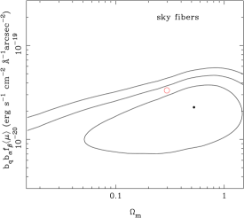
Appendix C: Sample tests
In this appendix we report on three consistency tests of our cross-correlation results. One test uses sky fibers to search for Ly emission instead of galaxy fibers, and the second looks at how the luminosity of the orginally targeted galaxy affects the quasar-Ly cross-correlation. The third test investigates how quasar luminosity affects the cross-correlation.
C.1 Sky fibers
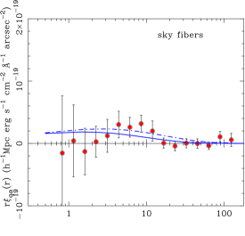
Ideally one would like to be able to use fibers positioned on random areas of the sky to carry out intensity mapping, without needing to worry about subtracting a foreground galaxy. This approach is being carried out for example by HETDEX (Blanc et al. 2011). In our case, however, there are a number of such random fibers which were obtained for each plate, to use in sky-subtraction. The number of fibers available for use to use is 146065, approximately 15% as many as there are galaxy fibers in our fiducial dataset. We have taken these sky fibers and carried out the quasar-Ly cross-correlation of Equation 1. The calculation was the same as in the fiducial case, including subtraction of a background from fiber (Figure 1).
We show the results for for the sky fibers in Figure 24. We can see that the datapoints appear to be consistent with the trend delineated by the best fit to the fiducial computation (also shown, as a dash-dotted line), although the measurement is much noisier. We fit the same CDM linear correlation function as was carried out in Section 3.2 and show the best fit parameters and confidence contours in Figure 23. We find erg s-1 cm-2 Å-1 arcsec-2 and . Here we can see that there that the confidence contours are very wide, and that the clustering signal is present at only the confidence level. The results are also consistent with the results from the fiducial sample at the 1.5 level. At present therefore, this shows that the use of galaxy and sky fibers in computing the cross-correlation is approximately equivalent, although the uncertainty is obviously large.
In the future, it would arguably be best to use randomly distributed fibers to carry out the cross-correlation, to avoid any potential selection biases. In the current sample case these biases are below the level of detectability, but one can imagine two types of bias, related to the fact that galaxy fibers are selected in regions of above average sky brightness and sky fibers selected to be in regions of below average sky brightness. Both effects could in principle bias the measurement of Ly surface brightness in opposite directions. We now carry out a further test to constrain this effect, by splitting the spectra into two halves bases on target LRG luminosity.
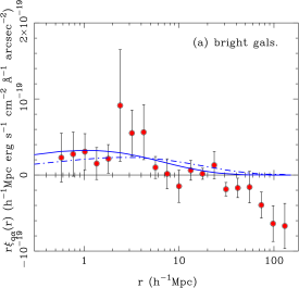
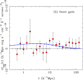
C.2 Sample split by galaxy luminosity
We divide the galaxy spectrum sample into two halves, based on the measured SDSS band luminosity (no k-correction was applied). One half consists of galaxies above the median luminosity of the whole dataset ( erg s-1), and the other half those below it. The median r band luminosities of the halves are erg s-1 and erg s-1
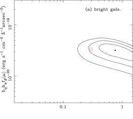
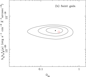
We note that the LRG galaxy surface brightnesses measured from BOSS spectra are of order erg s-1 cm-2 Å-1 arcsec-2, approximately orders of magnitude brighter than the mean Ly surface brightness that we have measured in Section 5. We therefore expect that it is unlikely that regions of excess background Ly surface brightness could have caused certain LRGs to be preferentially selected and therefore bias our measurements.
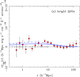
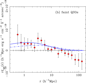
We measure the quasar-Ly cross correlation for the two samples of spectra and show the results in Figure 25. Both subsamples show evidence of clustering that is consistent with the CDM model shape and the fiducial amplitude. This can be seen in a quantitative manner from Figure 26, where we show the fit parameters. We find = erg s-1 cm-2 Å-1 arcsec-2, for the bright galaxy spectra and = erg s-1 cm-2 Å-1 arcsec-2, for the faint galaxy spectra. Both samples are consistent with the amplitude of the fiducial result at the level (the fiducial sample fractional error bar is bar for fixed ). This indicates that any bias present in the mean surface brightness due to fiber target selection is likely to be at the level or less.
C.3 Sample split by quasar luminosity
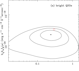
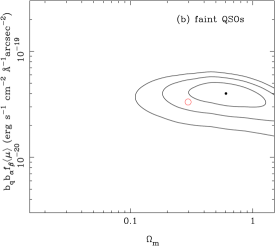
A potential source of Ly emission clustered with quasars is recombination radiation from dense IGM systems illuminated by the quasars themselves (e.g., Kollmeier et al. 2010). We have made an estimate of the amplitude of this signal in Section 6 and find it likely that it is much smaller than the signal from star forming galaxies clustered with the quasar. One way of testing this directly is by splitting the sample into high and low luminosity quasars and then measuring the signal for each. We note that this test can also function as a diagnostic for stray light contamination from quasars, as any stray light should be correlated with quasar luminosity.
In this section we do this, measuring the subsample of quasars with SDSS r band luminosity above the median, and with the subsample with luminosities below the median. The median luminosity of the bright subsample is 3.45 times the median luminosity of the faint sample, and the median redshifts of the quasars in each are and respectively.
We can see in Figures 27 that the results for two subsamples do not look very different. In particular if the quasar luminosities were causing significant fluorescent emission from nearby IGM material one might expect the brighter subsample to exhibit a steeper on small scales, which is not the case. From Figure 28 we can see that the fit parameters for the bright subsample are within of the fiducial result and the faint subsample within . The amplitude of parameter ( ) (for Planck ) is actually slightly lower for the bright subsample, being erg s-1 cm-2 Å-1 arcsec-2, whereas for the faint subsample it is erg s-1 cm-2 Å-1 arcsec-1. Given that the quasar subsamples are different in luminosities by a factor of 3.45 one would expect there to be a significant difference the results in the opposite direction if quasar properties were significantly affecting the large-scale Ly intensity around them. As mentioned above, this lack of dependence on quasar luminosity is also strong evidence that stray light from quasars scattered in the spectrograph is not contaminating our measured cross-correlation signal.
C.4 Other: sample split by fiber position in spectrograph
It is possible to imagine other sample tests based on various observational parameters, which could help to identify sources of systematic error. One such test is to split the sample into two subsets based on position of fibers in the spectrograph. Of the 1000 fibers, those labelled with numbers 100-400 and 600-900 are positioned towards the center of the spectrograph and the rest are positioned more towards the edge. The reason for such a test is that the optical quality of the instrument cameras degrades towards the edge, and this might affect the signal to noise ratio and/or cause other problems.
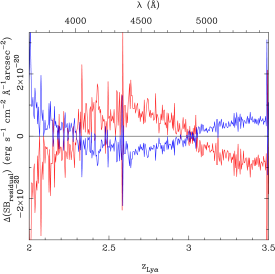
We carry out this split, and find that the average residual flux after subtraction of the model LRG spectra is somewhat different for the two subsamples. The residual flux for the fiducial sample was plotted in Figure 1, where we saw that it fluctuated between approximately for most of the relevant redshift range. In Figure 29 we plot for each subsample (edge and center) , the residual flux for the subsample minus the residual flux for the fiducial sample. We can see that there are indeed differences- the residual flux in fibers close to the edge of the cameras is systematically higher than the fiducial sample (and the center of camera sample) by over the wavelength range Å. As this covers the important Ly redshift range , this could indeed have consequences for our measurements.
Using the appropriate mean residual flux for each subsample, we compute the quasar-Ly emission cross-correlation . It should be noted that the subsamples are not quite the same size (there are 400 “edge” fibers per plate vs 600 “center” fibers). We fit the usual CDM model parameters and find = erg s-1 cm-2 Å-1 arcsec-2, and for the central fibers and = erg s-1 cm-2 Å-1 arcsec-2, and for the edge fibers. The central fiber results are within 1 of the fiducial results, but the edge fiber parameters have larger errors and are 2.5 below the fiducial results. We have also tried averaging the results from the two subsamples before fitting and find fit parameters consistent at the level with the fiducial results.
This test appears to show that the degradation of the optical quality of the spectrograph cameras close to the edge of their field of view does affect our ability to measure . Given this degradation, it is reasonable to expect that the error bars for the edge sample are underestimated and that this may account for the 2.5 difference with the fiducial sample. The fibers close to the center of camera sample appears to be responsible for most of our ability to determine . This information should be useful for future measurements of this type, but we do not use it to effect any changes to the fiducial analysis in this paper.