Additive Sweeping Preconditioner for the Helmholtz Equation

Abstract

We introduce a new additive sweeping preconditioner for the Helmholtz equation based on the perfect matched layer (PML). This method divides the domain of interest into thin layers and proposes a new transmission condition between the subdomains where the emphasis is on the boundary values of the intermediate waves. This approach can be viewed as an effective approximation of an additive decomposition of the solution operator. When combined with the standard GMRES solver, the iteration number is essentially independent of the frequency. Several numerical examples are tested to show the efficiency of this new approach.

Keyword. Helmholtz equation, perfectly matched layers, preconditioners, high frequency waves.

AMS subject classifications. 65F08, 65N22, 65N80.

1 Introduction

Let the domain of interest be $D=(0,1)^{d}$ where $d=2,3$. The Helmholtz equation is

$$\Delta u(x)+\dfrac{\omega^{2}}{c^{2}(x)}u(x)=f(x),\quad\forall x\in D,$$ (1)

where $u(x)$ is the time-independent wave field generated by the time-independent force $f(x)$, $\omega$ is the angular frequency and $c(x)$ is the velocity field. Commonly used boundary conditions are the approximations of the Sommerfeld radiation condition. By rescaling the system, we assume $c_{\min}\leq c(x)\leq c_{\max}$ where $c_{\min}$ and $c_{\max}$ are of $\Theta(1)$. Then $\omega/(2\pi)$ is the typical wave number and $\lambda=2\pi/\omega$ is the typical wavelength.

Solving the equation numerically is challenging in high frequency settings for two reasons. First, in most applications, the equation is discretized with at least a constant number of points per wavelength, which makes the number of points in each direction $n=\Omega(\omega)$ and the total degree of freedom $N=n^{d}=\Omega(\omega^{d})$ very large. Second, the system is highly indefinite and has a very oscillatory Green’s function, which makes most of the classical iterative methods no longer effective.

There has been a sequence of papers on developing iterative methods for solving (1). The AILU method by Gander and Nataf [10] is the first to use the incomplete LU factorization to precondition the equation. Engquist and Ying [6, 7] developed a series of sweeping preconditioners based on approximating the inverse of the Schur complements in the LDU factorization and obtained essentially $\omega$-independent iteration numbers. In [15], Stolk proposed a domain decomposition method based on the PML which constructs delicate transmission conditions between the subdomains by considering the “pulses” generated by the intermediate waves. In [19], Vion and Geuzaine proposed a double sweep preconditioner based on the Dirichlet-to-Neumann (DtN) map and several numerical simulations of the DtN map were compared. In [2, 3], Chen and Xiang introduced a source transfer domain decomposition method which emphasizes on transferring the sources between the subdomains. In [20], Zepeda-Núñez and Demanet developed a novel domain decomposition method for the 2D case by pairing up the waves and their normal derivatives at the boundary of the subdomains and splitting the transmission of the waves into two directions. Most recently in [13], Liu and Ying proposed a recursive sweeping preconditioner for 3D Helmholtz problems. Other progresses includes [14, 18, 16, 17] and we refer to [8] by Erlangga and [9] by Ernst and Gander for a complete discussion.

Inspired by [15] and these previous approaches, we propose a new domain decomposition method in this paper which shares some similarities with [7, 15]. The novelty of this new approach is that the transmission conditions are built with the boundary values of the intermediate waves directly. For each wave field on the subdomains, we divide it into three parts – the waves generated by the force to the left of the subdomain, to the right of the subdomain, and within the subdomain itself. This corresponds to an $L+D+U$ decomposition of the Green’s matrix $G$ as the sum of its lower triangular part, upper triangular part and diagonal part. This is why we call this new preconditioner the additive sweeping preconditioner.

The rest of this paper is organized as follows. First in Section 2 we use the 1D case to illustrate the idea of the method. Then in Section 3 we introduce the preconditioner in 2D and present the 2D numerical results. Section 4 discusses the 3D case. Conclusions and some future directions are provided in Section 5.

2 1D Illustration

We use the PML[1, 4, 12] to simulate the Sommerfeld condition. The PML introduces the auxiliary functions

$$\sigma(x) :=\begin{dcases}\dfrac{C}{\eta}\left(\dfrac{x-\eta}{\eta}\right)^{2},\quad&x\in[0,\eta),\\ 0,\quad&x\in[\eta,1-\eta],\\ \dfrac{C}{\eta}\left(\dfrac{x-1+\eta}{\eta}\right)^{2},\quad&x\in(1-\eta,1],\end{dcases}$$

$$s(x) :=\left(1+\,\mathrm{i}\dfrac{\sigma(x)}{\omega}\right)^{-1},$$

where C is an appropriate positive constant independent of $\omega$, and $\eta$ is the PML width which is typically around one wavelength.

The Helmholtz equation with PML in 1D is

$$\begin{dcases}\left((s(x)\dfrac{\,\mathrm{d}}{\,\mathrm{d}x})^{2}+\dfrac{\omega^{2}}{c^{2}(x)}\right)u(x)=f(x),\quad\forall x\in(0,1),\\ u(0)=0,\\ u(1)=0.\end{dcases}$$

We discretize the system with step size $h=1/(n+1)$, then $n$ is the degree of freedom. With the standard central difference numerical scheme the discretized equation is

$$\dfrac{s_{i}}{h}\left(\dfrac{s_{i+1/2}}{h}(u_{i+1}-u_{i})-\dfrac{s_{i-1/2}}{h}(u_{i}-u_{i-1})\right)+\dfrac{\omega^{2}}{c_{i}^{2}}u_{i}=f_{i},\quad\forall 1\leq i\leq n,$$ (2)

where the subscript $i$ means that the corresponding function is evaluated at $x=ih$.

We denote Equation (2) as $A\boldsymbol{u}=\boldsymbol{f}$, where $\boldsymbol{u}$ and $\boldsymbol{f}$ are the discrete array of the wave field and the force

$$\boldsymbol{u}:=[u_{1},\dots,u_{n}]^{T},\quad\boldsymbol{f}:=[f_{1},\dots,f_{n}]^{T}.$$

In 1D, $A$ is tridiagonal and Equation (2) can be solved without any difficulty. However, here we are aiming at an approach which can be generalized to higher dimensions so the rest of this section takes another point of view to solve (2) instead of exploiting the sparsity structure of $A$ directly.

With the Green’s matrix $G=A^{-1}$, $\boldsymbol{u}$ can be written as $\boldsymbol{u}=G\boldsymbol{f}$. Now let us divide the discrete grid into $m$ parts. We assume that $\eta=\gamma h$ and $n=2\gamma+mb-2$ where $\gamma$ and $b$ are some small constants and $m$ is comparable to $n$, and we define

$$X_{1} :=\{ih:1\leq i\leq\gamma+b-1\},$$

$$X_{p} :=\{ih:\gamma+(p-1)b\leq i\leq\gamma+pb-1\},\quad p=2,\dots,m-1,$$

$$X_{m} :=\{ih:\gamma+(m-1)b\leq i\leq 2\gamma+mb-2\},$$

which means, $X_{1}$ is the leftmost part containing the left PML of the original problem and a small piece of grid with $b$ points, $X_{m}$ is the rightmost part containing the right PML and a grid of $b$ points, and $X_{p},p=2,\dots,m-1$ are the middle parts each of which contains $b$ points. $\boldsymbol{u}_{p}$ and $\boldsymbol{f}_{p}$ are defined as the restrictions of $\boldsymbol{u}$ and $\boldsymbol{f}$ on $X_{p}$ for $p=1,\dots,m$, respectively,

$$\boldsymbol{u}_{1} :=[u_{1},\dots,u_{\gamma+b-1}]^{T},$$

$$\boldsymbol{u}_{p} :=[u_{\gamma+(p-1)b},\dots,u_{\gamma+pb-1}]^{T},\quad p=2,\dots,m-1,$$

$$\boldsymbol{u}_{m} :=[u_{\gamma+(m-1)b},\dots,u_{2\gamma+mb-2}]^{T},$$

$$\boldsymbol{f}_{1} :=[f_{1},\dots,f_{\gamma+b-1}]^{T},$$

$$\boldsymbol{f}_{p} :=[f_{\gamma+(p-1)b},\dots,f_{\gamma+pb-1}]^{T},\quad p=2,\dots,m-1,$$

$$\boldsymbol{f}_{m} :=[f_{\gamma+(m-1)b},\dots,f_{2\gamma+mb-2}]^{T}.$$

Then $u=Gf$ can be written as

$$\begin{bmatrix}\boldsymbol{u}_{1}\\ \boldsymbol{u}_{2}\\ \vdots\\ \boldsymbol{u}_{m}\end{bmatrix}=\begin{bmatrix}G_{1,1}&G_{1,2}&\ldots&G_{1,m}\\ G_{2,1}&G_{2,2}&\ldots&G_{2,m}\\ \vdots&\vdots&&\vdots\\ G_{m,1}&G_{m,2}&\ldots&G_{m,m}\end{bmatrix}\begin{bmatrix}\boldsymbol{f}_{1}\\ \boldsymbol{f}_{2}\\ \vdots\\ \boldsymbol{f}_{m}\end{bmatrix}.$$

By introducing $\boldsymbol{u}_{p,q}:=G_{p,q}\boldsymbol{f}_{q}$ for $1\leq p,q\leq m$, one can write $\boldsymbol{u}_{p}=\sum_{q=1}^{m}\boldsymbol{u}_{p,q}$. The physical meaning of $\boldsymbol{u}_{p,q}$ is the contribution of the force $\boldsymbol{f}_{q}$ defined on the grid $X_{q}$ acting upon the grid $X_{p}$. If we know the matrix $G$, the computation of $\boldsymbol{u}_{p,q}$ can be carried out directly. However, computing $G$, or even applying $G$ to the vector $\boldsymbol{f}$, is computationally expensive. The additive sweeping method circumvent this difficulty by approximating the blocks of $G$ sequentially and the idea works in higher dimensions. In what follows, we shall use $\tilde{\boldsymbol{u}}_{p,q}$ to denote the approximations of $\boldsymbol{u}_{p,q}$.

2.1 Approximating $\boldsymbol{u}_{p,q}$ with auxiliary PMLs

2.1.1 Wave generated by $\boldsymbol{f}_{1}$

The components ${\boldsymbol{u}}_{p,1}$ for $p=1,\dots,m$ can be regarded as a sequence of right-going waves generated by $\boldsymbol{f}_{1}$. Note that the boundary condition of the system is the approximated Sommerfeld condition. If we assume that the reflection during the transmission of the wave is negligible, then, to approximate $\boldsymbol{u}_{1,1}$, we can simply put an artificial PML on the right of the grid $X_{1}$ to solve a much smaller problem, since the domain of interest here is only $X_{1}$ (see Figure 2(b)). To be precise, we define

$$\sigma_{1}^{M}(x) :=\begin{dcases}\dfrac{C}{\eta}\left(\dfrac{x-\eta}{\eta}\right)^{2},\quad&x\in[0,\eta),\\ 0,\quad&x\in[\eta,\eta+(b-1)h],\\ \dfrac{C}{\eta}\left(\dfrac{x-(\eta+(b-1)h)}{\eta}\right)^{2},\quad&x\in(\eta+(b-1)h,2\eta+(b-1)h],\end{dcases}$$

$$s_{1}^{M}(x) :=\left(1+\,\mathrm{i}\dfrac{\sigma_{1}^{M}(x)}{\omega}\right)^{-1}.$$

We consider a subproblem on the auxiliary domain $D_{1}^{M}:=(0,2\eta+(b-1)h)$

$$\begin{dcases}\left((s_{1}^{M}(x)\dfrac{\,\mathrm{d}}{\,\mathrm{d}x})^{2}+\dfrac{\omega^{2}}{c^{2}(x)}\right)v(x)=g(x),\quad&\forall x\in D_{1}^{M},\\ v(x)=0,\quad&\forall x\in\partial D_{1}^{M}.\end{dcases}$$

With the same discrete numerical scheme and step size $h$, we have the corresponding discrete system $H_{1}^{M}\boldsymbol{v}=\boldsymbol{g}$ on the extended grid

$$X_{1}^{M}:=\{ih:1\leq i\leq 2\gamma+b-2\}.$$

Figure 1 shows a graphical view of $X_{1}^{M}$, as well as other extended grids which we will see later.

With the discrete system $H_{1}^{M}\boldsymbol{v}=\boldsymbol{g}$, we can define an operator $\tilde{G}_{1}^{M}:\boldsymbol{y}\to\boldsymbol{z}$, which is an approximation of $G_{1,1}$, by the following:

1. Introduce a vector $\boldsymbol{g}$ defined on $X_{1}^{M}$ by setting $\boldsymbol{y}$ to $X_{1}$ and zero everywhere else.

2. Solve $H_{1}^{M}\boldsymbol{v}=\boldsymbol{g}$ on $X_{1}^{M}$.

3. Set $\boldsymbol{z}$ as the restriction of $\boldsymbol{v}$ on $X_{1}$.

Then $\tilde{\boldsymbol{u}}_{1,1}$ can be set as

$$\tilde{\boldsymbol{u}}_{1,1}:=\tilde{G}_{1}^{M}\boldsymbol{f}_{1}.$$

Figure 1: This figure shows how the grids $X_{p}$ are extended with auxiliary PMLs.

Once we have computed $\tilde{\boldsymbol{u}}_{1,1}$, we can use the right boundary value of $\tilde{\boldsymbol{u}}_{1,1}$ to compute $\tilde{\boldsymbol{u}}_{2,1}$ by introducing an auxiliary PML on the right of $X_{2}$ and solving the boundary value problem with the left boundary value at $x=(\gamma+b-1)h$ equal to the right boundary value of $\tilde{\boldsymbol{u}}_{1,1}$. The same process can be repeated to compute $\tilde{\boldsymbol{u}}_{p+1,1}$ by exploiting the right boundary value of $\tilde{\boldsymbol{u}}_{p,1}$ recursively for $p=2,\dots,m-1$ (see Figure 2(c)). In the following context of this section, we introduce notations $g^{L},g^{R}$ for a vector array $\boldsymbol{g}=[g_{1},\dots,g_{s}]^{T}$ by

$$g^{L}:=g_{1},\quad g^{R}:=g_{s},$$

where $g^{L}$ and $g^{R}$ should be interpreted as the leftmost and the rightmost element of the array $\boldsymbol{g}$.

(a) The wave $\boldsymbol{u}_{1}$ (shown as the gray arrow) generated by $\boldsymbol{f}_{1}$.

(b) $\tilde{\boldsymbol{u}}_{1,1}$ is computed by introducing an auxiliary PML on the right of $X_{1}$. The dotted gray arrow stands for the restriction of ${\boldsymbol{u}}_{1}$ on $X_{2}\cup\dots\cup X_{m}$, which is to be approximated.

(c) $\tilde{\boldsymbol{u}}_{p,1}$ for $p=2,\dots,m$ are computed sequentially.

(d) $\tilde{\boldsymbol{u}}_{p,m}$ for $p=m,\dots,1$ are computed sequentially.

(e) $\tilde{\boldsymbol{u}}_{p,q}$ are computed for $p=q$ first, and then for $p=q+1,\dots,m$ and for $p=q-1,\dots,1$ sequentially.

Figure 2: This figure shows how $\tilde{\boldsymbol{u}}_{p,q}$ are generated. The direction of the arrows indicates the computing orders of the approximating waves.

To formalize the definition of $\tilde{\boldsymbol{u}}_{p,1}$ for each $p=2,\dots,m$, we introduce the auxiliary domain $D_{p}^{R}$, which will be defined below, to simulate the right-transmission of the waves. The superscript $R$ means that the auxiliary domain is intended for approximating the right-going waves. The left boundary of $D_{p}^{R}$ will be denoted as $\partial^{L}D_{p}^{R}$, on which the boundary value will be used to approximate the wave transmission as we shall see. We also extend $X_{p}$ with an auxiliary PML on the right to form an extended grid $X_{p}^{R}$ (see Figure 1), which corresponds the discretization of $D_{p}^{R}$. To be specific, we define

$$D_{p}^{R} :=(\eta+((p-1)b-1)h,2\eta+(pb-1)h),$$

$$\partial^{L}D_{p}^{R} :=\{\eta+((p-1)b-1)h\},$$

$$X_{p}^{R} :=\{ih:\gamma+(p-1)b\leq i\leq 2\gamma+pb-2\}.$$

Note that the grid $X_{m}^{R}$ is $X_{m}$ itself since $X_{m}$ already contains the original right PML region. The purpose to use the notation $X_{m}^{R}$ is to simplify the description of the algorithm.

For the PML on $D_{p}^{R}$, we define

$$\sigma_{p}^{R}(x) :=\begin{dcases}0,\quad&x\in[\eta+((p-1)b-1)h,\eta+(pb-1)h],\\ \dfrac{C}{\eta}\left(\dfrac{x-(\eta+(pb-1)h)}{\eta}\right)^{2},\quad&x\in(\eta+(pb-1)h,2\eta+(pb-1)h],\end{dcases}$$

$$s_{p}^{R} :=\left(1+\,\mathrm{i}\dfrac{\sigma_{p}^{R}(x)}{\omega}\right)^{-1}.$$

We consider the following subproblem

$$\begin{dcases}\left((s_{p}^{R}(x)\dfrac{\,\mathrm{d}}{\,\mathrm{d}x})^{2}+\dfrac{\omega^{2}}{c^{2}(x)}\right)v(x)=0,\quad&\forall x\in D_{p}^{R},\\ v(x)=w,\quad&\forall x\in\partial^{L}D_{p}^{R},\\ v(x)=0,\quad&\forall x\in\partial D_{p}^{R}\setminus\partial^{L}D_{p}^{R},\end{dcases}$$

where $w$ is the left boundary value of the unknown $v(x)$. We define $H_{p}^{R}\boldsymbol{v}=\boldsymbol{g}$ as the discretization of this problem on $X_{p}^{R}$ where the right-hand side $\boldsymbol{g}$ is given by $\boldsymbol{g}:=(-1/h^{2})[w,0,\dots,0]^{T}$ as a result of the central discretization. The subproblem $H_{p}^{R}\boldsymbol{v}=\boldsymbol{g}$ for each $p=2,\dots,m$ induces the approximation operator $\tilde{G}_{p}^{R}:w\to\boldsymbol{z}$ by the following procedure:

1. Set $\boldsymbol{g}=(-1/h^{2})[w,0,\dots,0]^{T}$.

2. Solve $H_{p}^{R}\boldsymbol{v}=\boldsymbol{g}$ on $X_{p}^{R}$.

3. Set $\boldsymbol{z}$ as the restriction of $\boldsymbol{v}$ on $X_{p}$.

Then $\tilde{\boldsymbol{u}}_{p,1}$ can be defined recursively for $p=2,\dots,m$ by

$$\tilde{\boldsymbol{u}}_{p,1}:=\tilde{G}_{p}^{R}\tilde{\boldsymbol{u}}_{p-1,1}^{R}.$$

Note that, the operator $\tilde{G}_{p}^{R}$ is not an approximation of the matrix block $G_{p,1}$, since $\tilde{G}_{p}^{R}$ maps the right boundary value of $\tilde{\boldsymbol{u}}_{p-1,1}$ to $\tilde{\boldsymbol{u}}_{p,1}$ while $G_{p,1}$ maps $\boldsymbol{f}_{1}$ to $\boldsymbol{u}_{p,1}$.

2.1.2 Wave generated by $\boldsymbol{f}_{m}$

The components ${\boldsymbol{u}}_{p,m}$ for $p=1,\dots,m$ can be regarded as a sequence of left-going waves generated by $\boldsymbol{f}_{m}$. The method for approximating them is similar to what was done for $\boldsymbol{f}_{1}$ (see Figure 2(d)). More specifically, for $\tilde{\boldsymbol{u}}_{m,m}$ we define

$$D_{m}^{M} :=(1-2\eta-(b-1)h,1),$$

$$X_{m}^{M} :=\{ih:(m-1)b+1\leq i\leq 2\gamma+mb-2\},$$

$$\sigma_{m}^{M}(x) :=\begin{dcases}\dfrac{C}{\eta}\left(\dfrac{x-(1-\eta-(b-1)h)}{\eta}\right)^{2},\quad&x\in[1-2\eta-(b-1)h,1-\eta-(b-1)h),\\ 0,\quad&x\in[1-\eta-(b-1)h,1-\eta],\\ \dfrac{C}{\eta}\left(\dfrac{x-(1-\eta)}{\eta}\right)^{2},\quad&x\in(1-\eta,1],\end{dcases}$$

$$s_{m}^{M}(x) :=\left(1+\,\mathrm{i}\dfrac{\sigma_{m}^{M}(x)}{\omega}\right)^{-1}.$$

We consider the continuous problem

$$\begin{dcases}\left((s_{m}^{M}(x)\dfrac{\,\mathrm{d}}{\,\mathrm{d}x})^{2}+\dfrac{\omega^{2}}{c^{2}(x)}\right)v(x)=g(x),\quad&\forall x\in D_{m}^{M},\\ v(x)=0,\quad&\forall x\in\partial D_{m}^{M},\end{dcases}$$

and define $H_{m}^{M}\boldsymbol{v}=\boldsymbol{g}$ as its discretization on $X_{m}^{M}$. The operator $\tilde{G}_{m}^{M}:\boldsymbol{y}\to\boldsymbol{z}$ can be defined as:

1. Introduce a vector $\boldsymbol{g}$ defined on $X_{m}^{M}$ by setting $\boldsymbol{y}$ to $X_{m}$ and zero everywhere else.

2. Solve $H_{m}^{M}\boldsymbol{v}=\boldsymbol{g}$ on $X_{m}^{M}$.

3. Set $\boldsymbol{z}$ as the restriction of $\boldsymbol{v}$ on $X_{m}$.

Then

$$\tilde{\boldsymbol{u}}_{m,m}:=\tilde{G}_{m}^{M}\boldsymbol{f}_{m}.$$

For each $\tilde{\boldsymbol{u}}_{p,m},p=1,\dots,m-1$, we introduce the auxiliary domain $D_{p}^{L}$, the right boundary $\partial^{R}D_{p}^{L}$, the extended grid $X_{p}^{L}$, and the corresponding PML functions $\sigma_{p}^{L}(x),s_{p}^{L}(x)$ as follows

$$D_{p}^{L} :=((p-1)bh,\eta+pbh),$$

$$\partial^{R}D_{p}^{L} :=\{\eta+pbh\},$$

$$X_{p}^{L} :=\{x_{i}:(p-1)b+1\leq i\leq\gamma+pb-1\},$$

$$\sigma_{p}^{L}(x) :=\begin{dcases}\dfrac{C}{\eta}\left(\dfrac{x-(\eta+(p-1)bh)}{\eta}\right)^{2},\quad&x\in[(p-1)bh,\eta+(p-1)bh),\\ 0,\quad&x\in[\eta+(p-1)bh,\eta+pbh],\end{dcases}$$

$$s_{p}^{L}(x) :=\left(1+\,\mathrm{i}\dfrac{\sigma_{p}^{L}(x)}{\omega}\right)^{-1},$$

and we consider the continuous problem

$$\begin{dcases}\left((s_{p}^{L}(x)\dfrac{\,\mathrm{d}}{\,\mathrm{d}x})^{2}+\dfrac{\omega^{2}}{c^{2}(x)}\right)v(x)=0,\quad&\forall x\in D_{p}^{L},\\ v(x)=w,\quad&\forall x\in\partial^{R}D_{p}^{L},\\ v(x)=0,\quad&\forall x\in\partial D_{p}^{L}\setminus\partial^{R}D_{p}^{L},\end{dcases}$$

where $y$ is the right boundary value of $v(x)$. Let $H_{p}^{L}\boldsymbol{v}=\boldsymbol{g}$ be its discretization on $X_{p}^{L}$ with $\boldsymbol{g}:=(-1/h^{2})[0,\dots,0,w]^{T}$. We introduce the operator $\tilde{G}_{p}^{L}:w\mapsto\boldsymbol{z}$ by:

1. Set $\boldsymbol{g}=(-1/h^{2})[0,\dots,0,w]^{T}$.

2. Solve $H_{p}^{L}\boldsymbol{v}=\boldsymbol{g}$ on $X_{p}^{L}$.

3. Set $\boldsymbol{z}$ as the restriction of $\boldsymbol{v}$ on $X_{p}$.

Then $\tilde{\boldsymbol{u}}_{p,m}$ can be defined recursively for $p=m-1,\dots,1$ by

$$\tilde{\boldsymbol{u}}_{p,m}:=\tilde{G}_{p}^{L}\tilde{\boldsymbol{u}}_{p+1,m}^{L}.$$

2.1.3 Wave generated by $\boldsymbol{f}_{q}$ for $q=2,\dots,m-1$

For each $q$, the components ${\boldsymbol{u}}_{p,q}$ for $p=1,\dots,m$ can be regarded as a sequence of left- and right-going waves generated by $\boldsymbol{f}_{q}$ (see Figure 2(e)). For $\tilde{\boldsymbol{u}}_{q,q}$, we introduce

$$D_{q}^{M} :=((q-1)bh,2\eta+(qb-1)h),$$

$$X_{q}^{M} :=\{x_{i}:(q-1)b+1\leq i\leq 2\gamma+qb-2\},$$

$$\sigma_{q}^{M}(x) :=\begin{dcases}\dfrac{C}{\eta}\left(\dfrac{x-(\eta+(q-1)bh)}{\eta}\right)^{2},\quad&x\in[(q-1)bh,\eta+(q-1)bh),\\ 0,\quad&x\in[\eta+(q-1)bh,\eta+(qb-1)h],\\ \dfrac{C}{\eta}\left(\dfrac{x-(\eta+(qb-1)h)}{\eta}\right)^{2},\quad&x\in(\eta+(qb-1)h,2\eta+(qb-1)h],\end{dcases}$$

$$s_{q}^{M}(x) :=\left(1+\,\mathrm{i}\dfrac{\sigma_{q}^{M}(x)}{\omega}\right)^{-1},$$

and define $H_{q}^{M}\boldsymbol{v}=\boldsymbol{g}$ as the discrete problem of the continuous problem

$$\begin{dcases}\left((s_{q}^{M}(x)\dfrac{\,\mathrm{d}}{\,\mathrm{d}x})^{2}+\dfrac{\omega^{2}}{c^{2}(x)}\right)v(x)=g(x),\quad&\forall x\in D_{q}^{M},\\ v(x)=0,\quad&\forall x\in\partial D_{q}^{M}.\end{dcases}$$

We introduce the operator $\tilde{G}_{q}^{M}:\boldsymbol{y}\to\boldsymbol{z}$ as:

1. Introduce a vector $\boldsymbol{g}$ defined on $X_{q}^{M}$ by setting $\boldsymbol{y}$ to $X_{q}$ and zero everywhere else.

2. Solve $H_{q}^{M}\boldsymbol{v}=\boldsymbol{g}$ on $X_{q}^{M}$.

3. Set $\boldsymbol{z}$ as the restriction of $\boldsymbol{v}$ on $X_{q}$.

Then

$$\tilde{\boldsymbol{u}}_{q,q}:=\tilde{G}_{q}^{M}\boldsymbol{f}_{q}.$$

Following the above discussion, the remaining components $\tilde{\boldsymbol{u}}_{p,q}$ are defined recursively as

$$\tilde{\boldsymbol{u}}_{p,q} :=\tilde{G}_{p}^{R}\tilde{\boldsymbol{u}}_{p-1,q}^{R},\quad\text{for }p=q+1,\dots,m,$$

$$\tilde{\boldsymbol{u}}_{p,q} :=\tilde{G}_{p}^{L}\tilde{\boldsymbol{u}}_{p+1,q}^{L},\quad\text{for }p=q-1,\dots,1.$$

2.2 Accumulating the boundary values

After all the above are done, an approximation of $\boldsymbol{u}_{p}$ is given by (see Figure 3(a))

$$\tilde{\boldsymbol{u}}_{p}:=\sum_{q=1}^{m}\tilde{\boldsymbol{u}}_{p,q},\quad p=1,\dots,m.$$

(a) $\tilde{\boldsymbol{u}}_{p}$ is a superposition of $\tilde{\boldsymbol{u}}_{p,q},q=1,\dots,m$.

(b) $\tilde{\boldsymbol{u}}_{p}$ is a superposition of $\tilde{\boldsymbol{u}}_{p,1:p-1}$, $\tilde{\boldsymbol{u}}_{p,p}$ and $\tilde{\boldsymbol{u}}_{p,p+1:m}$.

Figure 3: This figure shows how the boundary values are accumulated after each step. The thin arrows indicate the transmission directions of the waves. The bold, up-pointing arrows symbolizes that summing up the corresponding waves on $X_{p}$ gives the superposition wave $\tilde{\boldsymbol{u}}_{p}$.

In the algorithm described above, the computation of each component $\tilde{\boldsymbol{u}}_{p,q}$ requires a separate solution of a problem of form $H_{p}^{R}\boldsymbol{v}=\boldsymbol{g}$ or $H_{p}^{L}\boldsymbol{v}=\boldsymbol{g}$. Since there are $O(m^{2})$ such components, the algorithm is computationally expensive. A key observation is that the computation associated with each $p$ can be combined in one single shot by accumulating the boundary values of the waves. More precisely, we define

$$\tilde{\boldsymbol{u}}_{p,q_{1}:q_{2}}:=\sum_{t=q_{1}}^{q_{2}}\tilde{\boldsymbol{u}}_{p,t},$$

which is the total contribution of the waves generated by $\boldsymbol{f}_{q_{1}},\dots,\boldsymbol{f}_{q_{2}}$ restricted to the grid $X_{p}$. The quantity $\tilde{\boldsymbol{u}}_{p,1:p-1}$, which is the total right-going wave generated by $\boldsymbol{f}_{1},\dots,\boldsymbol{f}_{p-1}$ upon $X_{p}$, can be computed sequentially for $p=2,\dots,m$ without computing each component and then adding them together as we described above, as long as we accumulate the boundary values after each intermediate step. Specifically, we first compute $\tilde{\boldsymbol{u}}_{q,q}=\tilde{G}_{q}^{M}\boldsymbol{f}_{q}$ for $q=1,\dots,m$. This step is similar to what we did above. Then, to compute $\tilde{\boldsymbol{u}}_{p,1:p-1}$ we carry out the following steps

$$\tilde{\boldsymbol{u}}_{p,1:p-1}=\tilde{G}_{p}^{R}\tilde{\boldsymbol{u}}_{p-1,1:p-1}^{R},\quad\tilde{\boldsymbol{u}}_{p,1:p}^{R}=\tilde{\boldsymbol{u}}_{p,1:p-1}^{R}+\tilde{\boldsymbol{u}}_{p,p}^{R},\quad\text{for }p=2,\dots,m.$$

This means, before computing the total right-going wave $\tilde{\boldsymbol{u}}_{p+1,1:p}$ on subdomain $X_{p+1}$, the boundary values of the previous right-going waves, $\tilde{\boldsymbol{u}}_{p,1:p-1}^{R}$ and $\tilde{\boldsymbol{u}}_{p,p}^{R}$, are added together, so that the the current right-going wave $\tilde{\boldsymbol{u}}_{p+1,1:p}$ can be computed in one shot, eliminating the trouble of solving the subproblems for many times and adding the results together (see Figure 3(b)).

For the left going waves $\tilde{\boldsymbol{u}}_{p,p+1:m}$, a similar process gives rise to the recursive formula

$$\tilde{\boldsymbol{u}}_{p,p+1:m}=\tilde{G}_{p}^{L}\tilde{\boldsymbol{u}}_{p+1,p+1:m}^{L},\quad\tilde{\boldsymbol{u}}_{p,p:m}^{L}=\tilde{\boldsymbol{u}}_{p,p}^{L}+\tilde{\boldsymbol{u}}_{p,p+1:m}^{L},\quad\text{for }p=m-1,\dots,1.$$

Finally, each $\tilde{\boldsymbol{u}}_{p}$ can be computed by summing $\tilde{\boldsymbol{u}}_{p,1:p-1}$, $\tilde{\boldsymbol{u}}_{p,p}$ and $\tilde{\boldsymbol{u}}_{p,p+1:m}$ together (for the leftmost and the rightmost one, $\tilde{\boldsymbol{u}}_{1}$ and $\tilde{\boldsymbol{u}}_{m}$, only two terms need to be summed), i.e.,

$$\tilde{\boldsymbol{u}}_{1} =\tilde{\boldsymbol{u}}_{1,1}+\tilde{\boldsymbol{u}}_{1,2:m},$$

$$\tilde{\boldsymbol{u}}_{p} =\tilde{\boldsymbol{u}}_{p,1:p-1}+\tilde{\boldsymbol{u}}_{p,p}+\tilde{\boldsymbol{u}}_{p,p+1:m},\quad p=2,\dots,m-1,$$

$$\tilde{\boldsymbol{u}}_{m} =\tilde{\boldsymbol{u}}_{m,1:m-1}+\tilde{\boldsymbol{u}}_{m,m}.$$

We see that, by accumulating the boundary values after each intermediate step, we only need to solve $O(m)$ subproblems instead of $O(m^{2})$.

In this algorithm, the approximation $\tilde{\boldsymbol{u}}_{p}$ on each small subdomain is divided into three parts. From a matrix point of view, this is analogous to splitting the block matrix $G$ into its lower triangular part, diagonal part and upper triangular part, and then approximating each part as an operator to get the intermediate waves and then summing the intermediate results together. This is why we call it the additive sweeping method.

Equation (3) shows an analogy of this procedure, where the matrix $G$ is split into $3m-2$ blocks, each of which corresponds to a subproblem solving process:

$$\tilde{\boldsymbol{u}}_{q,q} \approx{\boldsymbol{u}}_{q,q}=G_{q,q}{\boldsymbol{f}}_{q},\quad q=1,\dots,m,$$

$$\tilde{\boldsymbol{u}}_{p,1:p-1} \approx{\boldsymbol{u}}_{p,1:p-1}=\sum_{q=1}^{p-1}G_{p,q}{\boldsymbol{f}}_{q},\quad p=2,\dots,m,$$

$$\tilde{\boldsymbol{u}}_{p,p+1:m} \approx{\boldsymbol{u}}_{p,p+1:m}=\sum_{q=p+1}^{m}G_{p,q}{\boldsymbol{f}}_{q},\quad p=1,\dots,m-1.$$

$$\begin{bmatrix}\boldsymbol{u}_{1}\\ \boldsymbol{u}_{2}\\ \ldots\\ \boldsymbol{u}_{m}\end{bmatrix}=\begin{bmatrix}\boldsymbol{u}_{1,1}+\boldsymbol{u}_{1,2:m}\\ \boldsymbol{u}_{2,1}+\boldsymbol{u}_{2,2}+\boldsymbol{u}_{2,3:m}\\ \ldots\\ \boldsymbol{u}_{m,1:m-1}+\boldsymbol{u}_{m,m}\end{bmatrix}=\left[\begin{array}[]{ccccc}\lx@intercol\hfil G_{1,1}\hfil\lx@intercol\vrule\lx@intercol&G_{1,2}&\dots&&G_{1,m}\\ \hline\cr G_{2,1}&\vrule\lx@intercol\hfil G_{2,2}\hfil\lx@intercol\vrule\lx@intercol&G_{2,3}&\ldots&G_{2,m}\\ \hline\cr&&\ldots&&\\ \hline\cr G_{m,1}&\ldots&\textbullet&G_{m,m-1}&\vrule\lx@intercol\hfil G_{m,m}\hfil\lx@intercol\end{array}\right]\begin{bmatrix}\boldsymbol{f}_{1}\\ \boldsymbol{f}_{2}\\ \ldots\\ \boldsymbol{f}_{m}\end{bmatrix}$$ (3)

When combined with standard iterative solvers, the approximation algorithm serves as a preconditioner for Equation (2) and it can be easily generalized to higher dimensions. In the following sections, we will discuss the details of the algorithm in 2D and 3D. To be structurally consistent, we will keep the notations for 2D and 3D the same with the 1D case without causing ambiguity. Some of the key notations and concepts are listed below as a reminder to the reader:

• $\{X_{p}\}_{p=1}^{m}$ The sliced partition of the discrete grid.

• $\{D_{q}^{M}\}_{q=1}^{m}$ The auxiliary domains with two-sided PML padding.

• $\{D_{p}^{R}\}_{p=2}^{m}$ The auxiliary domains with right-side PML padding.

• $\{D_{p}^{L}\}_{p=1}^{m-1}$ The auxiliary domains with left-side PML padding.

• $\{X_{q}^{M}\}_{q=1}^{m}$ $X_{q}$ with two-sided PML padding, the discretization of $D_{q}^{M}$.

• $\{X_{p}^{R}\}_{p=2}^{m}$ $X_{p}$ with right-side PML padding, the discretization of $D_{p}^{R}$.

• $\{X_{p}^{L}\}_{p=1}^{m-1}$ $X_{p}$ with left-side PML padding, the discretization of $D_{p}^{L}$.

• $\{\tilde{G}_{q}^{M}\}_{q=1}^{m}$  The auxiliary Green’s operators each of which maps the force on $X_{q}$ to the approximation of the wave field restricted to $X_{q}$.

• $\{\tilde{G}_{p}^{R}\}_{p=2}^{m}$  The auxiliary Green’s operators each of which maps the left boundary value to the approximated wave field restricted to $X_{p}$, which simulates the right-transmission of the waves.

• $\{\tilde{G}_{p}^{L}\}_{p=1}^{m-1}$  The auxiliary Green’s operators each of which maps the right boundary value to the approximated wave field restricted to $X_{p}$, which simulates the left-transmission of the waves.

3 Preconditioner in 2D

3.1 Algorithm

The domain of interest is $D=(0,1)^{2}$. We put PML on the two opposite sides of the boundary, $x_{2}=0$ and $x_{2}=1$, to illustrate the idea. The resulting equation is

$$\begin{dcases}\left(\partial_{1}^{2}+(s(x_{2})\partial_{2})^{2}+\dfrac{\omega^{2}}{c^{2}(x)}\right)u(x)=f(x),&\quad\forall x=(x_{1},x_{2})\in D,\\ u(x)=0,&\quad\forall x\in\partial D,\end{dcases}$$

We discretize $D$ with step size $h=1/(n+1)$ in each direction, which results the Cartesian grid

$$X:=\{(i_{1}h,i_{2}h):1\leq i_{1},i_{2}\leq n\},$$

and the discrete equation

$$\begin{gathered}\dfrac{s_{i_{2}}}{h}\left(\dfrac{s_{i_{2}+1/2}}{h}(u_{i_{1},i_{2}+1}-u_{i_{1},i_{2}})-\dfrac{s_{i_{2}-1/2}}{h}(u_{i_{1},i_{2}}-u_{i_{1},i_{2}-1})\right)\\ +\dfrac{u_{i_{1}+1,i_{2}}-2u_{i_{1},i_{2}}+u_{i_{1}-1,i_{2}}}{h^{2}}+\dfrac{\omega^{2}}{c_{i_{1},i_{2}}^{2}}u_{i_{1},i_{2}}=f_{i_{1},i_{2}},\quad\forall 1\leq i_{1},i_{2}\leq n,\end{gathered}$$ (4)

where the subscript $(i_{1},i_{2})$ means that the corresponding function is evaluated at $(i_{1}h,i_{2}h)$, and since $s(x_{2})$ is a function of $x_{2}$ only, we omit the $i_{1}$ subscript. $\boldsymbol{u}$ and $\boldsymbol{f}$ are defined to be the column-major ordering of the discrete array $u$ and $f$ on the grid $X$

$$\boldsymbol{u}:=[u_{1,1},\dots,u_{n,1},\dots,u_{n,n}]^{T},\quad\boldsymbol{f}:=[f_{1,1},\dots,f_{n,1},\dots,f_{n,n}]^{T}.$$

Now (4) can be written as $A\boldsymbol{u}=\boldsymbol{f}$.

We divide the grid into $m$ parts along the $x_{2}$ direction

$$X_{1} :=\{(i_{1}h,i_{2}h):1\leq i_{1}\leq n,1\leq i_{2}\leq\gamma+b-1\},$$

$$X_{p} :=\{(i_{1}h,i_{2}h):1\leq i_{1}\leq n,\gamma+(p-1)b\leq i_{2}\leq\gamma+pb-1\},\quad p=2,\dots,m-1,$$

$$X_{m} :=\{(i_{1}h,i_{2}h):1\leq i_{1}\leq n,\gamma+(m-1)b\leq i_{2}\leq 2\gamma+mb-2\},$$

and we define $\boldsymbol{u}_{p}$ and $\boldsymbol{f}_{p}$ as the column-major ordering restriction of $u$ and $f$ on $X_{p}$

$$\boldsymbol{u}_{1} :=[u_{1,1},\dots,u_{n,1},\dots,u_{n,\gamma+b-1}]^{T},$$

$$\boldsymbol{u}_{p} :=[u_{1,\gamma+(p-1)b},\dots,u_{n,\gamma+(p-1)b},\dots,u_{n,\gamma+pb-1}]^{T},\quad p=2,\dots,m-1,$$

$$\boldsymbol{u}_{m} :=[u_{1,\gamma+(m-1)b},\dots,u_{n,\gamma+(m-1)b},\dots,u_{n,2\gamma+mb-2}]^{T},$$

$$\boldsymbol{f}_{1} :=[f_{1,1},\dots,f_{n,1},\dots,f_{n,\gamma+b-1}]^{T},$$

$$\boldsymbol{f}_{p} :=[f_{1,\gamma+(p-1)b},\dots,f_{n,\gamma+(p-1)b},\dots,f_{n,\gamma+pb-1}]^{T},\quad p=2,\dots,m-1,$$

$$\boldsymbol{f}_{m} :=[f_{1,\gamma+(m-1)b},\dots,f_{n,\gamma+(m-1)b},\dots,f_{n,2\gamma+mb-2}]^{T},$$

then $\boldsymbol{u}=G\boldsymbol{f}$ for $G=A^{-1}$ can be written as

$$\begin{bmatrix}\boldsymbol{u}_{1}\\ \boldsymbol{u}_{2}\\ \vdots\\ \boldsymbol{u}_{m}\end{bmatrix}=\begin{bmatrix}G_{1,1}&G_{1,2}&\ldots&G_{1,m}\\ G_{2,1}&G_{2,2}&\ldots&G_{2,m}\\ \vdots&\vdots&&\vdots\\ G_{m,1}&G_{m,2}&\ldots&G_{m,m}\end{bmatrix}\begin{bmatrix}\boldsymbol{f}_{1}\\ \boldsymbol{f}_{2}\\ \vdots\\ \boldsymbol{f}_{m}\end{bmatrix}.$$

Auxiliary domains.

Following to the 1D case, the extended subdomains and the corresponding left and right boundaries are defined by

$$D_{q}^{M} =(0,1)\times((q-1)bh,2\eta+(qb-1)h),\quad q=1,\dots,m,$$

$$D_{p}^{R} =(0,1)\times(\eta+((p-1)b-1)h,2\eta+(pb-1)h),\quad p=2,\dots,m,$$

$$D_{p}^{L} =(0,1)\times((p-1)bh,\eta+pbh),\quad p=1,\dots,m-1,$$

$$\partial^{L}D_{p}^{R} =(0,1)\times\{\eta+((p-1)b-1)h\},\quad p=2,\dots,m,$$

$$\partial^{R}D_{p}^{L} =(0,1)\times\{\eta+pbh\},\quad p=1,\dots,m-1.$$

The extended grid for these domains are

$$X_{q}^{M} :=\{(i_{1}h,i_{2}h):1\leq i_{1}\leq n,(q-1)b+1\leq i_{2}\leq 2\gamma+qb-1\},\quad q=1,\dots,m,$$

$$X_{p}^{R} :=\{(i_{1}h,i_{2}h):1\leq i_{1}\leq n,\gamma+(p-1)b\leq i_{2}\leq 2\gamma+pb-2\},\quad p=2,\dots,m,$$

$$X_{p}^{L} :=\{(i_{1}h,i_{2}h):1\leq i_{1}\leq n,(p-1)b+1\leq i_{2}\leq\gamma+pb-1\},\quad p=1,\dots,m-1.$$

Auxiliary problems.

For $q=1,\dots,m$, we define $H_{q}^{M}\boldsymbol{v}=\boldsymbol{g}$ to be the discretization on $X_{q}^{M}$ of the problem

$$\begin{dcases}\left(\partial_{1}^{2}+(s_{q}^{M}(x_{2})\partial_{2})^{2}+\dfrac{\omega^{2}}{c^{2}(x)}\right)v(x)=g(x),\quad&\forall x\in D_{q}^{M},\\ v(x)=0,\quad&\forall x\in\partial D_{q}^{M}.\end{dcases}$$

For $p=2,\dots,m$, $H_{p}^{R}\boldsymbol{v}=\boldsymbol{g}$ is the discretization on $X_{p}^{R}$ of the problem

$$\begin{dcases}\left(\partial_{1}^{2}+(s_{p}^{R}(x_{2})\partial_{2})^{2}+\dfrac{\omega^{2}}{c^{2}(x)}\right)v(x)=0,\quad&\forall x\in D_{p}^{R},\\ v(x)=w(x_{1}),\quad&\forall x\in\partial^{L}D_{p}^{R},\\ v(x)=0,\quad&\forall x\in\partial D_{p}^{R}\setminus\partial^{L}D_{p}^{R},\end{dcases}$$

where $\boldsymbol{g}:=(-1/h^{2})[\boldsymbol{w}^{T},0,\dots,0]^{T}$ and $\boldsymbol{w}:=[w_{1},\dots,w_{n}]^{T}$ is the discrete value of $w(x_{1})$. Finally, for $p=1,\dots,m-1$, $H_{p}^{L}\boldsymbol{v}=\boldsymbol{g}$ is the discretization on $X_{p}^{L}$ of the problem

$$\begin{dcases}\left(\partial_{1}^{2}+(s_{p}^{L}(x_{2})\partial_{2})^{2}+\dfrac{\omega^{2}}{c^{2}(x)}\right)v(x)=0,\quad&\forall x\in D_{p}^{L},\\ v(x)=w(x_{1}),\quad&\forall x\in\partial^{R}D_{p}^{L},\\ v(x)=0,\quad&\forall x\in\partial D_{p}^{L}\setminus\partial^{R}D_{p}^{L},\end{dcases}$$

where $\boldsymbol{g}:=(-1/h^{2})[0,\dots,0,\boldsymbol{w}^{T}]^{T}$ and $\boldsymbol{w}:=[w_{1},\dots,w_{n}]^{T}$.

Auxiliary Green’s operators.

For $q=1,\dots,m$, we define $\tilde{G}_{q}^{M}:\boldsymbol{y}\mapsto\boldsymbol{z}$ to be the operator defined by the following operations:

1. Introduce a vector $\boldsymbol{g}$ defined on $X_{q}^{M}$ by setting $\boldsymbol{y}$ to $X_{q}$ and zero everywhere else.

2. Solve $H_{q}^{M}\boldsymbol{v}=\boldsymbol{g}$ on $X_{q}^{M}$.

3. Set $\boldsymbol{z}$ as the restriction of $\boldsymbol{v}$ on $X_{q}$.

For $p=2,\dots,m$, the operators $\tilde{G}_{p}^{R}:\boldsymbol{w}\mapsto\boldsymbol{z}$ is given by:

1. Set $\boldsymbol{g}=(-1/h^{2})[\boldsymbol{w}^{T},0,\dots,0]^{T}$.

2. Solve $H_{p}^{R}\boldsymbol{v}=\boldsymbol{g}$ on $X_{p}^{R}$.

3. Set $\boldsymbol{z}$ as the restriction of $\boldsymbol{v}$ on $X_{p}$.

Finally, for $p=1,\dots,m-1$, $\tilde{G}_{p}^{L}:\boldsymbol{w}\mapsto\boldsymbol{z}$ is defined as:

1. Set $\boldsymbol{g}=(-1/h^{2})[0,\dots,0,\boldsymbol{w}^{T}]^{T}$.

2. Solve $H_{p}^{L}\boldsymbol{v}=\boldsymbol{g}$ on $X_{p}^{L}$.

3. Set $\boldsymbol{z}$ as the restriction of $\boldsymbol{v}$ on $X_{p}$.

Putting together.

Similar to the previous section, we introduce the left boundary value $\boldsymbol{g}^{L}$ and the right boundary value $\boldsymbol{g}^{R}$ for a column-major ordering array $\boldsymbol{g}=[g_{1,1},\dots,g_{s_{1},1},\dots,g_{s_{1},s_{2}}]^{T}$ induced from some grid with size $s_{1}\times s_{2}$ by

$$\boldsymbol{g}^{L}:=[g_{1,1},\dots,g_{s_{1},1}]^{T},\quad\boldsymbol{g}^{R}:=[g_{1,s_{2}},\dots,g_{s_{1},s_{2}}]^{T}.$$

Then the approximations for $\boldsymbol{u}_{p},p=1,\dots,m$, can be defined step by step as

$$\tilde{\boldsymbol{u}}_{q,q} :=\tilde{G}_{q}^{M}\boldsymbol{f}_{q},\quad q=1,\dots,m,$$

$$\tilde{\boldsymbol{u}}_{p,1:p-1} :=\tilde{G}_{p}^{R}\tilde{\boldsymbol{u}}_{p-1,1:p-1}^{R},\quad\tilde{\boldsymbol{u}}_{p,1:p}^{R}:=\tilde{\boldsymbol{u}}_{p,1:p-1}^{R}+\tilde{\boldsymbol{u}}_{p,p}^{R},\quad\text{for }p=2,\dots,m,$$

$$\tilde{\boldsymbol{u}}_{p,p+1:m} :=\tilde{G}_{p}^{L}\tilde{\boldsymbol{u}}_{p+1,p+1:m}^{L},\quad\tilde{\boldsymbol{u}}_{p,p:m}^{L}:=\tilde{\boldsymbol{u}}_{p,p}^{L}+\tilde{\boldsymbol{u}}_{p,p+1:m}^{L},\quad\text{for }p=m-1,\dots,1,$$

$$\tilde{\boldsymbol{u}}_{1} :=\tilde{\boldsymbol{u}}_{1,1}+\tilde{\boldsymbol{u}}_{1,2:m},$$

$$\tilde{\boldsymbol{u}}_{p} :=\tilde{\boldsymbol{u}}_{p,1:p-1}+\tilde{\boldsymbol{u}}_{p,p}+\tilde{\boldsymbol{u}}_{p,p+1:m},\quad p=2,\dots,m-1,$$

$$\tilde{\boldsymbol{u}}_{m} :=\tilde{\boldsymbol{u}}_{m,1:m-1}+\tilde{\boldsymbol{u}}_{m,m}.$$

To solve the subproblems $H_{q}^{M}\boldsymbol{v}=\boldsymbol{g}$, $H_{p}^{R}\boldsymbol{v}=\boldsymbol{g}$ and $H_{p}^{L}\boldsymbol{v}=\boldsymbol{g}$, we notice that they are indeed quasi-1D problems since $\gamma$ and $b$ are some small constants. Therefore, for each one of them, we can reorder the system by grouping the elements along dimension 2 first and then dimension 1, which results a banded linear system that can be solved by the LU factorization efficiently. These factorization processes induce the factorizations for the operators $\tilde{G}_{q}^{M}$, $\tilde{G}_{p}^{R}$ and $\tilde{G}_{p}^{L}$ symbolically, which leads to our setup algorithm of the preconditioner in 2D as described in Algorithm 1 and the application algorithm as described in Algorithm 2.

Algorithm 1 Construction of the 2D additive sweeping preconditioner of the Equation (4). Complexity $=O(n^{2}(b+\gamma)^{3}/b)=O(N(b+\gamma)^{3}/b)$.

  for $q=1,\dots,m$ do

     Construct the LU factorization of $H_{q}^{M}$, which defines $\tilde{G}_{q}^{M}$.

  end for

  for $p=2,\dots,m$ do

     Construct the LU factorization of $H_{p}^{R}$, which defines $\tilde{G}_{p}^{R}$.

  end for

  for $p=1,\dots,m-1$ do

     Construct the LU factorization of $H_{p}^{L}$, which defines $\tilde{G}_{p}^{L}$.

  end for

Algorithm 2 Computation of $\tilde{\boldsymbol{u}}\approx G\boldsymbol{f}$ using the preconditioner from Algorithm 1. Complexity $=O(n^{2}(b+\gamma)^{2}/b)=O(N(b+\gamma)^{2}/b)$.

  for $q=1,\dots,m$ do

     $\tilde{\boldsymbol{u}}_{q,q}=\tilde{G}_{q}^{M}\boldsymbol{f}_{q}$

  end for

  for $p=2,\dots,m$ do

     $\tilde{\boldsymbol{u}}_{p,1:p-1}=\tilde{G}_{p}^{R}\tilde{\boldsymbol{u}}_{p-1,1:p-1}^{R}$$\tilde{\boldsymbol{u}}_{p,1:p}^{R}=\tilde{\boldsymbol{u}}_{p,1:p-1}^{R}+\tilde{\boldsymbol{u}}_{p,p}^{R}$

  end for

  for $p=m-1,\dots,1$ do

     $\tilde{\boldsymbol{u}}_{p,p+1:m}=\tilde{G}_{p}^{L}\tilde{\boldsymbol{u}}_{p+1,p+1:m}^{L}$$\tilde{\boldsymbol{u}}_{p,p:m}^{L}=\tilde{\boldsymbol{u}}_{p,p}^{L}+\tilde{\boldsymbol{u}}_{p,p+1:m}^{L}$

  end for

  $\tilde{\boldsymbol{u}}_{1}=\tilde{\boldsymbol{u}}_{1,1}+\tilde{\boldsymbol{u}}_{1,2:m}$

  for $p=2,\dots,m-1$ do

     $\tilde{\boldsymbol{u}}_{p}=\tilde{\boldsymbol{u}}_{p,1:p-1}+\tilde{\boldsymbol{u}}_{p,p}+\tilde{\boldsymbol{u}}_{p,p+1:m}$

  end for

  $\tilde{\boldsymbol{u}}_{m}=\tilde{\boldsymbol{u}}_{m,1:m-1}+\tilde{\boldsymbol{u}}_{m,m}$

To analyze the complexity, we note that, in the setup process, there are $O(n/b)$ subproblems, each of which is a quasi-1D problem with $O(\gamma+b)$ layers along the second dimension. Therefore, the setup cost of each subproblem by the LU factorization is $O(n(\gamma+b)^{3})$ and the application cost is $O(n(\gamma+b)^{2})$. So the total setup cost is $O(n^{2}(\gamma+b)^{3}/b)$. Besides, one needs to solve each subproblem once during the application process so the total application cost is $O(n^{2}(\gamma+b)^{2}/b)$.

There are some differences when implementing the method practically:

1. In the above setting, PMLs are put only on two opposite sides of the unit square for illustration purpose. In reality, PMLs can be put on other sides of the domain if needed. As long as there are two opposite sides with PML boundary condition, the method can be implemented.

2. The thickness of the auxiliary PMLs introduced in the interior part of the domain needs not to be the same with the thickness of the PML at the boundary. In fact, the thickness of the auxiliary PML is typically thinner in order to improve efficiency.

3. The widths of the subdomains are completely arbitrary and they need not to be the same. Practically, the widths can be chosen to be larger for subdomains where the velocity field varies heavily.

4. The symmetric version of the equation can be adopted to save memory and computational cost.

3.2 Numerical results

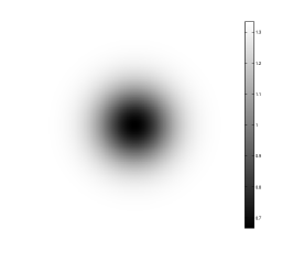
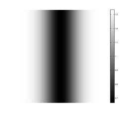
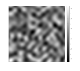
Here, we present some numerical results in 2D to illustrate the efficiency of the algorithm. The proposed method is implemented in MATLAB and the tests are performed on a 2.0 GHz computer with 256 GB memory. GMRES is used as the iterative solver with relative residual equal to $10^{-3}$ and restart value equal to $40$. PMLs are put on all sides of the unit square. The velocity fields tested are given in Figure 4:

1. A converging lens with a Gaussian profile at the center of the domain.

2. A vertical waveguide with a Gaussian cross-section.

3. A random velocity field.

Figure 4: The three velocity fields tested in 2D.

For each velocity field, two external forces are tested:

1. A Gaussian point source centered at $(1/2,1/8)$.

2. A Gaussian wave packet with wavelength comparable to the typical wavelength of the domain. The packet centers at $(1/8,1/8)$ and points to the direction $(1/\sqrt{2},1/\sqrt{2})$.

\begin{overpic}[width=195.12767pt]{2Daa.pdf} \put(40.0,6.0){force (a)} \end{overpic}

\begin{overpic}[width=195.12767pt]{2Dab.pdf} \put(40.0,6.0){force (b)} \end{overpic}

velocity field (a)			force (a)		force (b)
$\omega/(2\pi)$	$N$	$T_{\text{setup}}$	$N_{\text{iter}}$	$T_{\text{solve}}$	$N_{\text{iter}}$	$T_{\text{solve}}$
16	$127^{2}$	8.1669e$-$01	4	5.3199e$-$01	4	2.5647e$-$01
32	$255^{2}$	3.4570e$+$00	4	7.3428e$-$01	4	7.2807e$-$01
64	$511^{2}$	1.5150e$+$01	5	3.6698e$+$00	4	3.7239e$+$00
128	$1023^{2}$	6.2713e$+$01	5	1.6812e$+$01	4	1.6430e$+$01
256	$2047^{2}$	2.6504e$+$02	6	7.8148e$+$01	4	5.6936e$+$01

Table 1: Results for velocity field (a) in 2D. Solutions with $\omega/(2\pi)=32$ are presented.

\begin{overpic}[width=195.12767pt]{2Dba.pdf} \put(40.0,6.0){force (a)} \end{overpic}

\begin{overpic}[width=195.12767pt]{2Dbb.pdf} \put(40.0,6.0){force (b)} \end{overpic}

velocity field (b)			force (a)		force (b)
$\omega/(2\pi)$	$N$	$T_{\text{setup}}$	$N_{\text{iter}}$	$T_{\text{solve}}$	$N_{\text{iter}}$	$T_{\text{solve}}$
16	$127^{2}$	7.0834e$-$01	6	2.9189e$-$01	4	1.9408e$-$01
32	$255^{2}$	3.2047e$+$00	8	1.6147e$+$00	4	7.9303e$-$01
64	$511^{2}$	1.4079e$+$01	8	6.3057e$+$00	4	3.9008e$+$00
128	$1023^{2}$	6.0951e$+$01	8	2.9097e$+$01	4	1.5287e$+$01
256	$2047^{2}$	2.6025e$+$02	8	1.1105e$+$02	5	7.2544e$+$01

Table 2: Results for velocity field (b) in 2D. Solutions with $\omega/(2\pi)=32$ are presented.

\begin{overpic}[width=195.12767pt]{2Dca.pdf} \put(40.0,6.0){force (a)} \end{overpic}

\begin{overpic}[width=195.12767pt]{2Dcb.pdf} \put(40.0,6.0){force (b)} \end{overpic}

velocity field (c)			force (a)		force (b)
$\omega/(2\pi)$	$N$	$T_{\text{setup}}$	$N_{\text{iter}}$	$T_{\text{solve}}$	$N_{\text{iter}}$	$T_{\text{solve}}$
16	$127^{2}$	7.0495e$-$01	5	2.4058e$-$01	6	2.8347e$-$01
32	$255^{2}$	3.1760e$+$00	5	1.0506e$+$00	5	9.9551e$-$01
64	$511^{2}$	1.4041e$+$01	6	4.7083e$+$00	7	6.7852e$+$00
128	$1023^{2}$	6.1217e$+$01	6	1.8652e$+$01	6	1.9792e$+$01
256	$2047^{2}$	2.5762e$+$02	8	1.1214e$+$02	6	8.6936e$+$01

Table 3: Results for velocity field (c) in 2D. Solutions with $\omega/(2\pi)=32$ are presented.

In these tests, each typical wavelength is discretized with 8 points. The width of the PML at the boundary and the one of the PMLs introduced in the interior parts of the domain are both $9h$, i.e., $\gamma=9$. The number of layers in each interior subdomain is $b=8$, the number of layers in the leftmost subdomain is $b+\gamma-1=16$ and the one in the rightmost is $b+\gamma-2=15$.

We vary the typical wave number $\omega/(2\pi)$ and test the behavior of the algorithm. The test results are presented in Tables 1, 2 and 3. $T_{\text{setup}}$ is the setup time of the algorithm in seconds. $T_{\text{solve}}$ is the total solve time in seconds and $N_{\text{iter}}$ is the iteration number. From these tests we see that the setup time scales like $O(N)$ as well as the solve time per iteration, which is consistent with the algorithm complexity analysis. The iteration number remains constant or grows at most logarithmically, which shows the efficiency of the preconditioner.

4 Preconditioner in 3D

4.1 Algorithm

In this section we briefly state the preconditioner in 3D case. The domain of interest is $D=(0,1)^{3}$. PMLs are put on two opposite faces of the unit cube, $x_{3}=0$ and $x_{3}=1$, which results the equation

$$\begin{dcases}\left(\partial_{1}^{2}+\partial_{2}^{2}+(s(x_{3})\partial_{3})^{2}+\dfrac{\omega^{2}}{c^{2}(x)}\right)u(x)=f(x),&\quad\forall x=(x_{1},x_{2},x_{3})\in D,\\ u(x)=0,&\quad\forall x\in\partial D,\end{dcases}$$

Discretizing $D$ with step size $h=1/(n+1)$ gives the grid

$$X:=\{(i_{1}h,i_{2}h,i_{3}h):1\leq i_{1},i_{2},i_{3}\leq n\},$$

and the discrete equation

$$\begin{gathered}\dfrac{s_{i_{3}}}{h}\left(\dfrac{s_{i_{3}+1/2}}{h}(u_{i_{1},i_{2},i_{3}+1}-u_{i_{1},i_{2},i_{3}})-\dfrac{s_{i_{3}-1/2}}{h}(u_{i_{1},i_{2},i_{3}}-u_{i_{1},i_{2},i_{3}-1})\right)\\ +\dfrac{u_{i_{1}+1,i_{2},i_{3}}-2u_{i_{1},i_{2},i_{3}}+u_{i_{1}-1,i_{2},i_{3}}}{h^{2}}+\dfrac{u_{i_{1},i_{2}+1,i_{3}}-2u_{i_{1},i_{2},i_{3}}+u_{i_{1},i_{2}-1,i_{3}}}{h^{2}}\\ +\dfrac{\omega^{2}}{c_{i_{1},i_{2},i_{3}}^{2}}u_{i_{1},i_{2},i_{3}}=f_{i_{1},i_{2},i_{3}},\quad\forall 1\leq i_{1},i_{2}\leq n.\end{gathered}$$ (5)

$\boldsymbol{u}$ and $\boldsymbol{f}$ are defined as the column-major ordering of $u$ and $f$ on the grid $X$

$$\boldsymbol{u}:=[u_{1,1,1},\dots,u_{n,1,1},\dots,u_{n,n,1},\dots,u_{n,n,n}]^{T},\quad\boldsymbol{f}:=[f_{1,1,1},\dots,f_{n,1,1},\dots,f_{n,n,1},\dots,f_{n,n,n}].$$

$X$ is divided into $m$ parts along the $x_{3}$ direction

$$X_{1} :=\{(i_{1}h,i_{2}h,i_{3}h):1\leq i_{1}\leq n,1\leq i_{2}\leq n,1\leq i_{3}\leq\gamma+b-1\},$$

$$X_{p} :=\{(i_{1}h,i_{2}h,i_{3}h):1\leq i_{1}\leq n,1\leq i_{2}\leq n,\gamma+(p-1)b\leq i_{3}\leq\gamma+pb-1\},\quad p=2,\dots,m-1,$$

$$X_{m} :=\{(i_{1}h,i_{2}h,i_{3}h):1\leq i_{1}\leq n,1\leq i_{2}\leq n,\gamma+(m-1)b\leq i_{3}\leq 2\gamma+mb-2\}.$$

$\boldsymbol{u}_{p}$ and $\boldsymbol{f}_{p}$ are the column-major ordering restrictions of $u$ and $f$ on $X_{p}$

$$\boldsymbol{u}_{1} :=[u_{1,1,1},\dots,u_{n,1,1},\dots,u_{n,n,1},\dots,u_{n,n,\gamma+b-1}]^{T},$$

$$\boldsymbol{u}_{p} :=[u_{1,1,\gamma+(p-1)b},\dots,u_{n,1,\gamma+(p-1)b},\dots,u_{n,n,\gamma+(p-1)b},\dots,u_{n,n,\gamma+pb-1}]^{T},\quad p=2,\dots,m-1,$$

$$\boldsymbol{u}_{m} :=[u_{1,1,\gamma+(m-1)b},\dots,u_{n,1,\gamma+(m-1)b},\dots,u_{n,n,\gamma+(m-1)b},\dots,u_{n,n,2\gamma+mb-2}]^{T},$$

$$\boldsymbol{f}_{1} :=[f_{1,1,1},\dots,f_{n,1,1},\dots,f_{n,n,1},\dots,f_{n,n,\gamma+b-1}]^{T},$$

$$\boldsymbol{f}_{p} :=[f_{1,1,\gamma+(p-1)b},\dots,f_{n,1,\gamma+(p-1)b},\dots,f_{n,n,\gamma+(p-1)b},\dots,f_{n,n,\gamma+pb-1}]^{T},\quad p=2,\dots,m-1,$$

$$\boldsymbol{f}_{m} :=[f_{1,1,\gamma+(m-1)b},\dots,f_{n,1,\gamma+(m-1)b},\dots,f_{n,n,\gamma+(m-1)b},\dots,f_{n,n,2\gamma+mb-2}]^{T}.$$

Auxiliary domains.

The extended subdomains, the extended grids, and the corresponding left and right boundaries are defined by

$$D_{q}^{M} :=(0,1)\times(0,1)\times((q-1)bh,2\eta+(qb-1)h),\quad q=1,\dots,m,$$

$$D_{p}^{R} :=(0,1)\times(0,1)\times(\eta+((p-1)b-1)h,2\eta+(pb-1)h),\quad p=2,\dots,m,$$

$$D_{p}^{L} :=(0,1)\times(0,1)\times((p-1)bh,\eta+pbh),\quad p=1,\dots,m-1,$$

$$\partial^{L}D_{p}^{R} :=(0,1)\times(0,1)\times\{\eta+((p-1)b-1)h\},\quad p=2,\dots,m,$$

$$\partial^{R}D_{p}^{L} :=(0,1)\times(0,1)\times\{\eta+pbh\},\quad p=1,\dots,m-1,$$

$$X_{q}^{M} :=\{(i_{1}h,i_{2}h,i_{3}h):1\leq i_{1}\leq n,1\leq i_{2}\leq n,(q-1)b+1\leq i_{3}\leq 2\gamma+qb-1\},\quad q=1,\dots,m,$$

$$X_{p}^{R} :=\{(i_{1}h,i_{2}h,i_{3}h):1\leq i_{1}\leq n,1\leq i_{2}\leq n,\gamma+(p-1)b\leq i_{3}\leq 2\gamma+pb-2\},\quad p=2,\dots,m,$$

$$X_{p}^{L} :=\{(i_{1}h,i_{2}h,i_{3}h):1\leq i_{1}\leq n,1\leq i_{2}\leq n,(p-1)b+1\leq i_{3}\leq\gamma+pb-1\},\quad p=1,\dots,m-1.$$

Auxiliary problems.

For each $q=1,\dots,m$, $H_{q}^{M}\boldsymbol{v}=\boldsymbol{g}$ is defined as the discretization on $X_{q}^{M}$ of

$$\begin{dcases}\left(\partial_{1}^{2}+\partial_{2}^{2}+(s_{q}^{M}(x_{3})\partial_{3})^{2}+\dfrac{\omega^{2}}{c^{2}(x)}\right)v(x)=g(x),&\quad\forall x\in D_{q}^{M},\\ v(x)=0,&\quad\forall x\in\partial D_{q}^{M},\end{dcases}$$

For $p=2,\dots,m$, $H_{p}^{R}\boldsymbol{v}=\boldsymbol{g}$ is defined as the discretization on $X_{p}^{R}$ of

$$\begin{dcases}\left(\partial_{1}^{2}+\partial_{2}^{2}+(s_{p}^{R}(x_{3})\partial_{3})^{2}+\dfrac{\omega^{2}}{c^{2}(x)}\right)v(x)=0,\quad&\forall x\in D_{p}^{R},\\ v(x)=w(x_{1},x_{2}),\quad&\forall x\in\partial^{L}D_{p}^{R},\\ v(x)=0,\quad&\forall x\in\partial D_{p}^{R}\setminus\partial^{L}D_{p}^{R},\end{dcases}$$

where $\boldsymbol{g}:=(-1/h^{2})[\boldsymbol{w}^{T},0,\dots,0]^{T}$ and $\boldsymbol{w}:=[w_{1,1},\dots,w_{n,1},\dots,w_{n,n}]$ is the discrete boundary value. Finally, for $p=1,\dots,m-1$, $H_{p}^{L}\boldsymbol{v}=\boldsymbol{g}$ is the discretization on $X_{p}^{L}$ of

$$\begin{dcases}\left(\partial_{1}^{2}+\partial_{2}^{2}+(s_{p}^{L}(x_{3})\partial_{3})^{2}+\dfrac{\omega^{2}}{c^{2}(x)}\right)v(x)=0,\quad&\forall x\in D_{p}^{L},\\ v(x)=w(x_{1},x_{2}),\quad&\forall x\in\partial^{R}D_{p}^{L},\\ v(x)=0,\quad&\forall x\in\partial D_{p}^{L}\setminus\partial^{R}D_{p}^{L},\end{dcases}$$

where $\boldsymbol{g}:=(-1/h^{2})[0,\dots,0,\boldsymbol{w}^{T}]^{T}$ and $\boldsymbol{w}:=[w_{1,1},\dots,w_{n,1},\dots,w_{n,n}]$.

Auxiliary Green’s operators.

For $q=1,\dots,m$, $\tilde{G}_{q}^{M}:\boldsymbol{y}\mapsto\boldsymbol{z}$ is defined using the following operations:

1. Introduce a vector $\boldsymbol{g}$ defined on $X_{q}^{M}$ by setting $\boldsymbol{y}$ to $X_{q}$ and zero everywhere else.

2. Solve $H_{q}^{M}\boldsymbol{v}=\boldsymbol{g}$ on $X_{q}^{M}$.

3. Set $\boldsymbol{z}$ as the restriction of $\boldsymbol{v}$ on $X_{q}$.

For $p=2,\dots,m$, $\tilde{G}_{p}^{R}:\boldsymbol{w}\mapsto\boldsymbol{z}$ is given by:

1. Set $\boldsymbol{g}=(-1/h^{2})[\boldsymbol{w}^{T},0,\dots,0]^{T}$.

2. Solve $H_{p}^{R}\boldsymbol{v}=\boldsymbol{g}$ on $X_{p}^{R}$.

3. Set $\boldsymbol{z}$ as the restriction of $\boldsymbol{v}$ on $X_{p}$.

Finally, for $p=1,\dots,m-1$, the operators $\tilde{G}_{p}^{L}:\boldsymbol{w}\mapsto\boldsymbol{z}$ is introduced to be:

1. Set $\boldsymbol{g}=(-1/h^{2})[0,\dots,0,\boldsymbol{w}^{T}]^{T}$.

2. Solve $H_{p}^{L}\boldsymbol{v}=\boldsymbol{g}$ on $X_{p}^{L}$.

3. Set $\boldsymbol{z}$ as the restriction of $\boldsymbol{v}$ on $X_{p}$.

Putting together.

In the 3D case, $\boldsymbol{g}^{L}$ and $\boldsymbol{g}^{R}$ for the column-major ordering array
$\boldsymbol{g}=[g_{1,1,1},\dots,g_{s_{1},1,1},\dots,g_{s_{1},s_{2},1},\dots,g_{s_{1},s_{2},s_{3}}]^{T}$ induced from some 3D grid with size
$s_{1}\times s_{2}\times s_{3}$ are given by

$$\boldsymbol{g}^{L}:=[g_{1,1,1},\dots,g_{s_{1},1,1},\dots,g_{s_{1},s_{2},1}]^{T},\quad\boldsymbol{g}^{R}:=[g_{1,1,s_{3}},\dots,g_{s_{1},1,s_{3}},\dots,g_{s_{1},s_{2},s_{3}}]^{T}.$$

The subproblems $H_{q}^{M}\boldsymbol{v}=\boldsymbol{g}$, $H_{p}^{R}\boldsymbol{v}=\boldsymbol{g}$ and $H_{p}^{L}\boldsymbol{v}=\boldsymbol{g}$ are quasi-2D. To solve them, we group the elements along dimension 3 first, and then apply the nested dissection method[11, 5] to them, as in [7]. This gives the setup process of the 3D preconditioner in Algorithm 3 and the application process in Algorithm 4.

Algorithm 3 Construction of the 3D additive sweeping preconditioner of the system (5). Complexity $=O(n^{4}(b+\gamma)^{3}/b)=O(N^{4/3}(b+\gamma)^{3}/b)$.

  for $q=1,\dots,m$ do

     Construct the nested dissection factorization of $H_{q}^{M}$, which defines $\tilde{G}_{q}^{M}$.

  end for

  for $p=2,\dots,m$ do

     Construct the the nested dissection factorization of $H_{p}^{R}$, which defines $\tilde{G}_{p}^{R}$.

  end for

  for $p=1,\dots,m-1$ do

     Construct the the nested dissection factorization of $H_{p}^{L}$, which defines $\tilde{G}_{p}^{L}$.

  end for

Algorithm 4 Computation of $\tilde{\boldsymbol{u}}\approx G\boldsymbol{f}$ using the preconditioner from Algorithm 3. Complexity $=O(n^{3}\log n(b+\gamma)^{2}/b)=O(N\log N(b+\gamma)^{2}/b)$.

  for $q=1,\dots,m$ do

     $\tilde{\boldsymbol{u}}_{q,q}=\tilde{G}_{q}^{M}\boldsymbol{f}_{q}$

  end for

  for $p=2,\dots,m$ do

     $\tilde{\boldsymbol{u}}_{p,1:p-1}=\tilde{G}_{p}^{R}\tilde{\boldsymbol{u}}_{p-1,1:p-1}^{R}$$\tilde{\boldsymbol{u}}_{p,1:p}^{R}=\tilde{\boldsymbol{u}}_{p,1:p-1}^{R}+\tilde{\boldsymbol{u}}_{p,p}^{R}$

  end for

  for $p=m-1,\dots,1$ do

     $\tilde{\boldsymbol{u}}_{p,p+1:m}=\tilde{G}_{p}^{L}\tilde{\boldsymbol{u}}_{p+1,p+1:m}^{L}$$\tilde{\boldsymbol{u}}_{p,p:m}^{L}=\tilde{\boldsymbol{u}}_{p,p}^{L}+\tilde{\boldsymbol{u}}_{p,p+1:m}^{L}$

  end for

  $\tilde{\boldsymbol{u}}_{1}=\tilde{\boldsymbol{u}}_{1,1}+\tilde{\boldsymbol{u}}_{1,2:m}$

  for $p=2,\dots,m-1$ do

     $\tilde{\boldsymbol{u}}_{p}=\tilde{\boldsymbol{u}}_{p,1:p-1}+\tilde{\boldsymbol{u}}_{p,p}+\tilde{\boldsymbol{u}}_{p,p+1:m}$

  end for

  $\tilde{\boldsymbol{u}}_{m}=\tilde{\boldsymbol{u}}_{m,1:m-1}+\tilde{\boldsymbol{u}}_{m,m}$

For the algorithm analysis, we notice that each quasi-2D subproblem has $O(\gamma+b)$ layers along the third dimension. Therefore, the setup cost for each subproblem is $O((\gamma+b)^{3}n^{3})$ and the application cost is $O((\gamma+b)^{2}n^{2}\log n)$. Taking the total number of subproblems into account, the total setup cost for the 3D preconditioner is $O(n^{4}(b+\gamma)^{3}/b)$ and the total application cost is $O(n^{3}\log n(b+\gamma)^{2}/b)$.

4.2 Numerical results

Here we present the numerical results in 3D. All the settings and notations are kept the same with Section 3.2 unless otherwise stated. The PMLs are put on all sides of the boundary and the symmetric version of the equation is adopted to save memory cost. The PML width is $\eta=9h$ for the boundary and is $\eta_{\text{aux}}=5h$ for the interior auxiliary ones. The number of layers in each subdomain is $b=4$ for the interior ones, $b+\gamma-1=12$ for the leftmost one and $b+\gamma-2=11$ for the rightmost one.

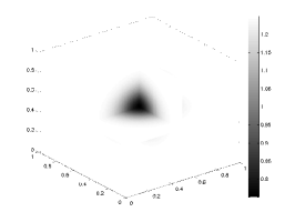
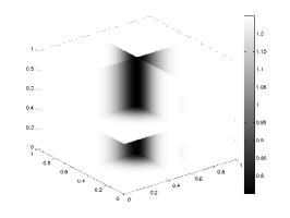
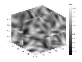
The velocity fields tested are (see Figure 5):

1. A converging lens with a Gaussian profile at the center of the domain.

2. A vertical waveguide with a Gaussian cross-section.

3. A random velocity field.

Figure 5: The three velocity fields tested in 3D.

The forces tested for each velocity field are:

1. A Gaussian point source centered at $(1/2,1/2,1/4)$.

2. A Gaussian wave packet with wavelength comparable to the typical wavelength of the domain. The packet centers at $(1/2,1/4,1/4)$ and points to the direction $(0,1/\sqrt{2},1/\sqrt{2})$.

\begin{overpic}[width=195.12767pt]{3Daa.pdf} \put(40.0,6.0){force (a)} \end{overpic}

\begin{overpic}[width=195.12767pt]{3Dab.pdf} \put(40.0,6.0){force (b)} \end{overpic}

velocity field (a)			force (a)		force (b)
$\omega/(2\pi)$	$N$	$T_{\text{setup}}$	$N_{\text{iter}}$	$T_{\text{solve}}$	$N_{\text{iter}}$	$T_{\text{solve}}$
5	$39^{3}$	2.3304e$+$01	3	2.9307e$+$00	4	3.7770e$+$00
10	$79^{3}$	3.2935e$+$02	3	3.6898e$+$01	4	4.6176e$+$01
20	$159^{2}$	4.2280e$+$03	4	4.3999e$+$02	4	4.6941e$+$02

Table 4: Results for velocity field (a) in 3D. Solutions with $\omega/(2\pi)=10$ at $x_{1}=0.5$ are presented.

\begin{overpic}[width=195.12767pt]{3Dba.pdf} \put(40.0,6.0){force (a)} \end{overpic}

\begin{overpic}[width=195.12767pt]{3Dbb.pdf} \put(40.0,6.0){force (b)} \end{overpic}

velocity field (b)			force (a)		force (b)
$\omega/(2\pi)$	$N$	$T_{\text{setup}}$	$N_{\text{iter}}$	$T_{\text{solve}}$	$N_{\text{iter}}$	$T_{\text{solve}}$
5	$39^{3}$	2.1315e$+$01	3	2.7740e$+$00	3	2.7718e$+$00
10	$79^{3}$	3.4256e$+$02	4	4.4286e$+$01	3	3.4500e$+$01
20	$159^{2}$	4.3167e$+$03	5	5.7845e$+$02	4	4.6462e$+$02

Table 5: Results for velocity field (b) in 3D. Solutions with $\omega/(2\pi)=10$ at $x_{1}=0.5$ are presented.

\begin{overpic}[width=195.12767pt]{3Dca.pdf} \put(40.0,6.0){force (a)} \end{overpic}

\begin{overpic}[width=195.12767pt]{3Dcb.pdf} \put(40.0,6.0){force (b)} \end{overpic}

velocity field (c)			force (a)		force (b)
$\omega/(2\pi)$	$N$	$T_{\text{setup}}$	$N_{\text{iter}}$	$T_{\text{solve}}$	$N_{\text{iter}}$	$T_{\text{solve}}$
5	$39^{3}$	2.1063e$+$01	4	3.8074e$+$00	4	3.7975e$+$00
10	$79^{3}$	3.4735e$+$02	4	4.4550e$+$01	4	4.5039e$+$01
20	$159^{2}$	4.3391e$+$03	4	4.4361e$+$02	5	5.8090e$+$02

Table 6: Results for velocity field (c) in 3D. Solutions with $\omega/(2\pi)=10$ at $x_{1}=0.5$ are presented.

The results are given in Tables 4, 5 and 6. From these tests we see that the iteration number grows mildly as the problem size grows. We also notice that the setup cost scales even better than $O(N^{4/3})$, mainly because MATLAB performs dense linear algebra operations in a parallel way, which gives some extra advantages to the nested dissection algorithm as the problem size grows.

5 Conclusion

In this paper, we proposed a new additive sweeping preconditioner for the Helmholtz equation based on the PML. When combined with the standard GMRES solver, the iteration number grows mildly as the problem size grows. The novelty of this approach is that the unknowns are split in an additive way and the boundary values of the intermediate results are utilized directly. The disadvantage is that, for each subdomains, three subproblems need to be built up, which is time consuming compared to [7] and [15]. However, the costly parts of the algorithm, i.e. the whole setup process and the solve processes of the subproblems $H_{q}^{M}\boldsymbol{v}=\boldsymbol{g}$, can be done in parallel. The only parts that must be implemented sequentially are the accumulations of the left-going and right-going waves, where only the solve processes of the subproblems $H_{p}^{L}\boldsymbol{v}=\boldsymbol{g}$ and $H_{p}^{R}\boldsymbol{v}=\boldsymbol{g}$ are involved, which are the cheapest parts of the algorithm. Besides, we think that the whole approximation process is simple and structurally clear from a physics point of view and the idea might be easy to be generalized to other equations.

There are also some other directions to make potential improvements. First, other numerical schemes of the equation and other approximations of the Sommerfeld radiation condition can be used to develop more efficient versions of this additive preconditioner. Second, the parallel version of the nested dissection algorithm can be combined to solve large scale problems. Last, in the 3D case, the quasi-2D subproblems can be solved recursively by sweeping along the $x_{2}$ direction with the same technique, which reduces the theoretical setup cost to $O(N)$ and the application cost to $O(N)$. However, compared to [7], the coefficient of the complexity in this new method is larger, so it is not clear whether or not the recursive approach will be more efficient practically. Nevertheless, it is of great theoretical interest to look into it.

References

- [1] J.-P. Berenger. A perfectly matched layer for the absorption of electromagnetic waves. J. Comput. Phys., 114(2):185–200, 1994.
- [2] Z. Chen and X. Xiang. A source transfer domain decomposition method for Helmholtz equations in unbounded domain. SIAM J. Numer. Anal., 51(4):2331–2356, 2013.
- [3] Z. Chen and X. Xiang. A source transfer domain decomposition method for Helmholtz equations in unbounded domain Part II: Extensions. Numer. Math. Theory Methods Appl., 6(3):538–555, 2013.
- [4] W. C. Chew and W. H. Weedon. A 3D perfectly matched medium from modified Maxwell’s equations with stretched coordinates. Microw. Opt. Techn. Let., 7(13):599–604, 1994.
- [5] I. S. Duff and J. K. Reid. The multifrontal solution of indefinite sparse symmetric linear equations. ACM Trans. Math. Software, 9(3):302–325, 1983.
- [6] B. Engquist and L. Ying. Sweeping preconditioner for the Helmholtz equation: Hierarchical matrix representation. Comm. Pure Appl. Math., 64(5):697–735, 2011.
- [7] B. Engquist and L. Ying. Sweeping preconditioner for the Helmholtz equation: Moving perfectly matched layers. Multiscale Model. Simul., 9(2):686–710, 2011.
- [8] Y. A. Erlangga. Advances in iterative methods and preconditioners for the Helmholtz equation. Arch. Comput. Methods Eng., 15(1):37–66, 2008.
- [9] O. G. Ernst and M. J. Gander. Why it is difficult to solve Helmholtz problems with classical iterative methods. In Numerical Analysis of Multiscale Problems, volume 83 of Lect. Notes Comput. Sci. Eng., pages 325–363. Springer, Heidelberg, 2012.
- [10] M. J. Gander and F. Nataf. AILU for Helmholtz problems: A new preconditioner based on the analytic parabolic factorization. J. Comput. Acoust., 9(4):1499–1506, 2001.
- [11] A. George. Nested dissection of a regular finite element mesh. SIAM J. Numer. Anal., 10(2):345–363, 1973.
- [12] S. G. Johnson. Notes on Perfectly Matched Layers (PMLs). Lecture notes, Massachusetts Institute of Technology, Massachusetts, 2008.
- [13] F. Liu and L. Ying. Recursive Sweeping Preconditioner for the 3D Helmholtz Equation. ArXiv e-prints, Feb. 2015.
- [14] J. Poulson, B. Engquist, S. Li, and L. Ying. A parallel sweeping preconditioner for heterogeneous 3D Helmholtz equations. SIAM J. Sci. Comput., 35(3):C194–C212, 2013.
- [15] C. C. Stolk. A rapidly converging domain decomposition method for the Helmholtz equation. J. Comput. Phys., 241(0):240 – 252, 2013.
- [16] P. Tsuji, B. Engquist, and L. Ying. A sweeping preconditioner for time-harmonic Maxwell’s equations with finite elements. J. Comput. Phys., 231(9):3770–3783, 2012.
- [17] P. Tsuji, J. Poulson, B. Engquist, and L. Ying. Sweeping preconditioners for elastic wave propagation with spectral element methods. ESAIM Math. Model. Numer. Anal., 48(2):433–447, 2014.
- [18] P. Tsuji and L. Ying. A sweeping preconditioner for Yee’s finite difference approximation of time-harmonic Maxwell’s equations. Front. Math. China, 7(2):347–363, 2012.
- [19] A. Vion and C. Geuzaine. Double sweep preconditioner for optimized Schwarz methods applied to the Helmholtz problem. J. Comput. Phys., 266(0):171 – 190, 2014.
- [20] L. Zepeda-Núñez and L. Demanet. The method of polarized traces for the 2D Helmholtz equation. ArXiv e-prints, Oct. 2014.