Prestellar Core Formation, Evolution, and Accretion from Gravitational Fragmentation in Turbulent Converging Flows
Abstract
We investigate prestellar core formation and accretion based on three-dimensional hydrodynamic simulations. Our simulations represent local pc regions within giant molecular clouds where a supersonic turbulent flow converges, triggering star formation in the post-shock layer. We include turbulence and self-gravity, applying sink particle techniques, and explore a range of inflow Mach number . Two sets of cores are identified and compared: -cores are identified of a time snapshot in each simulation, representing dense structures in a single cloud map; -cores are identified at their individual time of collapse, representing the initial mass reservoir for accretion. We find that cores and filaments form and evolve at the same time. At the stage of core collapse, there is a well-defined, converged characteristic mass for isothermal fragmentation that is comparable to the critical Bonner-Ebert mass at the post-shock pressure. The core mass functions (CMFs) of -cores show a deficit of high-mass cores () compared to the observed stellar initial mass function (IMF). However, the CMFs of -cores are similar to the observed CMFs and include many low-mass cores that are gravitationally stable. The difference between -cores and -cores suggests that the full sample from observed CMFs may not evolve into protostars. Individual sink particles accrete at a roughly constant rate throughout the simulations, gaining one -core mass per free-fall time even after the initial mass reservoir is accreted. High-mass sinks gain proportionally more mass at late times than low-mass sinks. There are outbursts in accretion rates, resulting from clumpy density structures falling into the sinks.
Subject headings:
ISM: structure –– methods: numerical –– stars: formation — stars: luminosity function, mass function –– turbulence1. Introduction
Dense molecular cores form in the last step of giant molecular cloud (GMC) fragmentation and are the cradles of single stars or close binary systems (McKee & Ostriker 2007; André et al. 2014). These cores provide the initial mass reservoir and set the local environment of star formation. Understanding core formation and the core mass function (CMF) is important for characterizing the initial conditions of star and planet formation, and explaining the origin of the stellar initial mass function (IMF, see review of Offner et al. 2014).
Cores emerge in dense regions of GMCs, the dynamics of which are governed by turbulence, gravity, and magnetic fields (Dobbs et al. 2014). Although supersonic turbulence provides support for GMCs on global scales, it compresses gas to high densities in local regions where gravitational collapse can rapidly occur (Ballesteros-Paredes et al. 2007; McKee & Ostriker 2007). Strong turbulence in GMCs can also accelerate ambipolar diffusion and aid in the creation of magnetically supercritical cores (Nakamura & Li 2005, 2008; Kudoh & Basu 2008, 2011; Chen & Ostriker 2012). However, in the situation where the large-scale GMC is magnetically supercritical, simulations show that anisotropic core formation via magnetic field-aligned flows results in similar core masses to the unmagnetized case (Chen & Ostriker 2014). In this paper, we focus on core formation and subsequent collapse and accretion using turbulent, unmagnetized simulations.
Cores are at the bottom of the hierarchy in a GMC, and are often associated with dense filaments seen in dust continuum and molecular lines. Observations show many pressure-confined gravitationally stable cores within clouds (and filaments), which may later become gravitationally unstable (Lada et al. 2008; André et al. 2010; Schisano et al. 2014). High resolution observations by Herschel Space Observatory indicate that gravitationally bound cores are mainly embedded along thermally super-critical filaments (André et al. 2010; Molinari et al. 2010; Schisano et al. 2014), i.e., those with mass per unit length exceeding (Ostriker 1964). This is in apparent agreement with the theoretical conclusion that self-gravitating filaments are unstable to longitudinal perturbations (Nagasawa 1987; Inutsuka & Miyama 1992, 1997), which would allow them to fragment into dense cores. However, the most unstable scale is several times the filament diameter, which would produce cores more massive than observed. Also, the two-step scenario in which filaments first form and then subsequently fragment into cores can be altered with the presence of large-amplitude turbulence, because the nonlinear perturbations produced by turbulence allow structures at many scales to grow simultaneously. With numerical simulations, it is possible to follow the temporal evolution of developing structures, and simulations with turbulence show that filaments and cores develop at the same time rather than in sequence (Gong & Ostriker 2011; Van Loo et al. 2014; Chen & Ostriker 2014, see also §3.1.1 in this paper).
Observationally, cores are divided into two categories: starless cores, and protostellar cores/Class 0 objects (di Francesco et al. 2007; André et al. 2009). Among the starless cores, a further classification is of prestellar cores, which are strongly gravitationally bound and centrally concentrated; the balance of other starless cores are the opposite: they appear to be largely pressure-confined rather than strongly gravitationally bound, and are not strongly centrally concentrated. Protostellar cores/Class 0 objects are gravitationally bound and contain embedded protostars/young stellar objects (YSOs). It is generally thought that these categories represent cores at different evolutionary stages: pressure-confined starless cores gain mass and turn into gravitationally bound prestellar cores, which finally collapse and become protostellar cores. However, in practice, prestellar cores are often not distinguished from other starless cores in observations. Some starless cores may even be transient structures that will never collapse to form protostars. Numerical simulation made it possible to check whether observed pressure-confined cores are likely to become unstable at a later time.
Many theoretical studies have investigated individual core evolution, beginning with the semi-analytical work of Larson (1969), Penston (1969), and Shu (1977). Based on isothermal simulations with supersonic converging flows, Gong & Ostriker (2009) identified four stages of core evolution: core building, core collapse, envelope infall, and late accretion. In the core building stage, the core gains mass from its environment, gradually becoming more centrally concentrated. For the spherical case, shock-bounded cores collapse when the central-to-edge pressure ratio is similar to that of a critical Bonnor-Ebert equilibrium sphere (Ebert 1955; Bonnor 1956), which has mass
| (1) | ||||
Here is external pressure at the edge of the core; is the mean core density; the core’s temperature; and is the internal sound speed in the core. After the core collapses, the internal density structure approaches the well-known Larson-Penston solution (Larson 1969; Penston 1969, hereafter LP)
| (2) |
where is the distance from the core center. This asymptotic state is reached regardless of the dynamical evolution leading up to collapse (see discussion and references in Gong & Ostriker 2009, 2011, hereafter GO09 and GO11); in particular, cores formed by supersonic flows approach the LP solution during collapse. Collapse leads to creation of an opaque core and then a protostar at the center, with a surrounding rotating disk (Shu et al. 1987). Subsequently, the dense envelope falls onto the protostar via an inside-out gravitationally-induced rarefaction wave (Shu 1977; Hunter 1977). GO09 define the late accretion stage as the period after the rarefaction wave has propagated beyond the region where the LP profile holds, and most of the original core mass has fallen into the center (the protostar/disk). The characteristic timescale for the core collapse and the envelope infall stages is the free-fall time
| (3) |
This is similar to the lifetime of prestellar and protostellar cores in observations (André et al. 2014).
Empirical measurement of CMFs from extinction and continuum mapping suggest the mass distribution has a similar shape to the IMF, but with the characteristic core mass shifted upward by a factor of (e.g., Alves et al. 2007; Nutter & Ward-Thompson 2007; Könyves et al. 2010). However, observed CMFs often include transient structures that may not collapse later, and the core masses obtained from observations can be dependent on the specific core finding algorithm applied (e.g., gaussclumps (Stutzki & Guesten 1990); clumpfind (Williams et al. 1994); getsources (Men’shchikov et al. 2010)). Although core identification based directly on surface density maps is somewhat ambiguous due to the arbitrary definition of the core boundary, use of the gravitational potential removes some of this ambiguity (Smith et al. 2009; Gong & Ostriker 2011). Analytical theories of the CMF (see review of Offner et al. 2014) focus on gravitationally bound cores. In this work, we identify two sets of cores: The first set is comparable to structures seen in a GMC at a given instant in time, and includes a range of evolutionary stages (both weakly and strongly bound). The second set represents cores seen at a fixed evolutionary state, the time of protostar formation. We address the differences between the two sets, and implications for interpretation of observations.
Even if every observed core were to collapse, evolution after core formation could further change the relation between the CMF and IMF. At a minimum, fragmentation into binaries and multiples due to rapid rotation, and mass loss due to protostellar outflows, complicates any mapping from the CMF to the IMF. In addition, a concern in the theoretical literature has been that there may be no preferred scale for isothermal fragmentation such that gravitational fragmentation in GMCs must depend crucially on non-isothermal effects (Martel et al. 2006; Krumholz 2014). This concern arises in part because an isothermal filament with mass per unit length greater than can collapse towards its axis without fragmenting, leading to infinite density (Inutsuka & Miyama 1997), and in part because homologous collapse of a sphere would lead to ever smaller Jeans masses and possible sub-fragmentation until stopped by non-isothermal effects (Hoyle 1953).
In fact, core collapse is non-homologous, such that the hierarchical fragmentation envisioned by Hoyle (1953) does not occur. However, disks that form around protostars are known to undergo excessive fragmentation and overproduce brown dwarfs if stellar heating is not included in simulations (Bate 2009). Here, we argue that the problem of excessive disk fragmentation in isothermal models can be distinguished form whether there is a well-defined CMF from gravoturbulent fragmentation of an isothermal cloud. We shall show that the characteristic core mass converges with increasing resolution (and threshold of sink particle creation) in our simulations. In reality, of course, GMCs and cores are not isothermal, but have temperature variations between K, with observationally inferred temperatures dropping toward the center of the cores (e.g., Marsh et al. 2014; Roy et al. 2014). However, the isothermal approximation is an adequate first limit from cloud to core scales. Radiation feedback and significant non-isothermal effects become important subsequent to core collapse, in the accretion disks around protostars.
In this paper, we present our results on prestellar core formation and collapse based on a large suite of three-dimensional numerical simulations. Our simulations model a local (pc) region of GMCs where a supersonic turbulent flow converges, inducing star formation in the post-shock layer. We adopt the same model of a supersonic and isothermal converging flow with turbulent perturbations as in GO11. As in GO11, we see filamentary structures form at the same time as dense cores. While the models of GO11 were halted when the first core collapsed, here we apply the sink particle implementation of Gong & Ostriker (2013) to trace the evolution at later times. We also explore a wider range of inflow Mach numbers (). Using simulations with varying numerical resolution, we show that the characteristic core mass at the time of collapse is well defined. We measure the statistical properties of cores, especially the CMF, and compare to the observed CMF and IMF. We are also able to trace the accretion rate of individual sink particles, and explore its time variation and dependence on core masses.
The outline of this paper is as follows. We describe our numerical methods and model parameters in §2. In §3, we present our results of overall evolution (§3.1), convergence of isothermal fragmentation (§3.2), core properties and CMF (§3.3), and sink particle accretion (§3.4). Finally §4 summarizes our conclusions.
2. Methods and Parameters
2.1. Numerical Methods
2.1.1 Basic Equations and Algorithms
The numerical simulations presented in this paper are conducted with the Athena code (Stone et al. 2008; Stone & Gardiner 2009), on a three dimensional (3D) Cartesian grid, using the van Leer (MUSCL-Hancock type) integrator, the HLLC Riemann solver, and second-order spatial reconstruction. The code solves for the self-gravity in planar geometry, with open boundary condition in the vertical () direction, and periodic boundary conditions in the horizontal ( and ) directions, using the fast Fourier transformation (FFT) method developed by Koyama & Ostriker (2009). Sink particles as implemented by Gong & Ostriker (2013) are included, and allow us to track the system evolution after individual cores collapse.
The equations solved for the gas are the conservation of mass and momentum:
| (4) |
| (5) |
and the Poisson equation:
| (6) |
where is the density, the velocity, the pressure, the gravitational potential of the gas, and the gravitational potential associated with the sink particles. For simplicity, we adopt an isothermal equation of state for the gas:
| (7) |
where is the isothermal sound speed of molecular gas with solar metallicity; the temperature; and the mass of the hydrogen atom.
The sink particle implementation of Gong & Ostriker (2013) is briefly summarized here. Our sink particle creation criteria require a local potential minimum and the density threshold set by the Larson-Penston profile in Equation (2) at a distance from the center:
| (8) |
here is the simulation cell size. Previously, §4.3 of Gong & Ostriker (2013) compared different criteria for sink particle creation (cf. Bate et al. 1995; Krumholz et al. 2004; Federrath et al. 2010; Padoan & Nordlund 2011), including the Truelove density threshold (Truelove et al. 1997), additional checks for converging flow and a gravitationally bound state, and found no differences in sink particle evolution. In our algorithm, there is a moving control volume centered on the cell containing each sink particle that acts similar to the ghost zones of the simulation domain. At every time step, the density and momentum of the cells inside each control volume are reset by extrapolation of the surrounding non-sink zones. The gas mass and momentum accretion onto each sink particle are calculated based on the sum over all fluxes returned by the Riemann solver at the outer surfaces of the sink control volume. Flows onto sink particles due to shifting of the control volume are also included. Sink particle positions and velocities are advanced in time via a leapfrog integrator. The gravitational potential from and the forces on sink particles are computed using a particle mesh method with a TSC kernal (Hockney & Eastwood 1981). Sink particles merge if their control volumes overlap.
2.1.2 Problem Specification and Units
We used the prescription of converging supersonic flow with turbulent perturbations following GO11 and Gong & Ostriker (2013). The models represent a localized ( scale) region in a turbulent GMC where the large scale velocity field converges and pre-stellar cores form in the post-shock dense gas.
The model setup consists of supersonic flow augmented with turbulent velocity perturbations, converging to the mid-plane from and directions at an average velocity of and . The inflowing gas has the same spectrum of turbulent perturbations as the initial conditions (see below), i.e., the cloud “outer scales” are treated as maintaining a fixed turbulent amplitude. There is no explicit turbulent driving within the box, although turbulence can be driven by shock instabilities. In our parameter survey, the Mach number values are 2, 4, 8 and 16. The initial density is set equal to the code unit (see below), as is the density of the converging flow from the boundaries. The boundaries in and directions are periodic.
We apply velocity perturbations for both the whole domain initially and the inflowing gas subsequently, following the prescription of GO11. The scaling law of the velocity field represents the observed linewidth-size relation in GMCs over a range of scales111Note, however, that at small scales where the turbulence is subsonic, it may follow a shallower Kolmogorov power law. (McKee & Ostriker 2007):
| (9) |
However, the timescale for the turbulence to relax at the largest scales, attaining self-consistent density and velocity perturbations, is longer than the inflow time from the boundaries. Thus, although the turbulence is not fully self-consistent, it serves to produce density perturbations that then evolve to collapse gravitationally.
Assuming the cloud-scale supersonic turbulence provides both the kinetic support of the cloud against its self-gravity and the large-scale converging flow with the virial parameter , GO11 show (their Equation (43) and (44)) that the Mach number of the converging flow can be related to the cloud’s size and Jeans length as . With the scaling of the velocity in Equation (9), the amplitude of velocity perturbations at the box scale can be written as 222In a global model, for which , one can show that this reduces to .. This corresponds to the “high-amplitude” perturbation simulations in GO11. In this paper, we adopt 10% of the above values for velocity perturbations, corresponding to the “low-amplitude” case in GO11. Thus, the largest velocity perturbation in a simulation is limited by
| (10) |
where is the horizontal ( and direction) box size. Note that for the Mach numbers and box size we use, although the average inflow velocity is highly supersonic, the velocity perturbations within the domain are subsonic.
We choose to focus on the low-amplitude perturbation case for two reasons: Firstly, we wish to concentrate on the local details of collapse produced by converging flows. For realistic GMC conditions, and the velocity perturbations at scales are small compared to the inflow motion , which means a post-shock layer with simple geometry would form; this situation is amenable to local simulations. However, for completeness, we wish to explore a range of values down to , and at low the velocity perturbations at scales would be comparable to inflow speeds. In this case, there would no longer be a post-shock layer with simple geometry, so that global simulations would be more suitable than local. By reducing the perturbation amplitude, we can use local models for all . Secondly, we are limited by computational power in practice, and the CPU time required for a simulation run is increased in high amplitude cases. Also, bigger simulation boxes and higher resolutions are required when the post-shock layer does not have a simple geometry and shows more complicated dynamics, increasing the necessary number of zones.
Nonetheless, it is important to address how the level of turbulence affects the core formation process. We therefore conducted two simulations with high-amplitude perturbations (see Section 2.2 for model parameters), and compare to the low-amplitude cases.
The code unit of density represents the average ambient density in a GMC flowing into the region in which stars will form. For this reference density, a characteristic spatial scale for gravitational instability is the Jeans length
| (11) |
The corresponding Jeans mass is
| (12) |
and Jeans time is
| (13) |
We use the Jeans length, mass, and time at the unperturbed density as the code units for length, mass, and time: , and . In making comparison to observations, another useful quantity is the surface density integrated along the z-direction through the domain
| (14) |
where .
To convert code units of length, mass and time to physical units, one may choose an appropriate mean density, (where ), and a temperature . This allows consideration of GMCs with a range of properties. Many GMCs are observed to be self-gravitating, such that the virial parameter is order-unity, where is the large-scale velocity dispersion along any direction. Defining the density of the cloud as and the surface density as so that , we can substitute and (assuming that the inflow Mach number is related to the large-scale GMC’s turbulence level), to obtain
| (15) |
| (16) |
| (17) |
and
| (18) |
These forms are useful because observations of GMCs measure surface density and Mach number more directly than volume density. Many of the best-studied local dark clouds and inner-galaxy GMCs have surface density , although clouds in more extreme environments such as the Galactic center and ultra-luminous infrared galaxies (ULIRGs) have higher (Dobbs et al. 2014). Table 1 lists the two different ways of translating code units to physical parameters in molecular clouds.
2.1.3 Core Finding Method
The cores in the simulations are identified using the GRID core finding method developed by GO11: the region belonging to a core is defined by the largest closed contour of the gravitational potential field around the corresponding local potential minimum that contains no other local minimum. Within each core, we further define the bound core region as all the material that has the sum of gravitational energy and thermal energy negative.333The gravitational and thermal energy density in each zone is , where is the gravitational potential at the core boundary, and . We have also defined kinetically bound cores with the volume integral of less than zero, where is the kinetic energy of the gas. We found that most cores are mainly supported by thermal pressure with , even in tests with high-amplitude turbulence perturbation. The cores are often not spherical, so we define an effective radius of a core with volume as . For the core properties such as mass, radius, and density, we use the notation , , and for cores defined by gravitational potential alone, and , , and for bound cores with .
To compare the physical properties of cores at different stages of evolution, two sets of cores are identified using different strategies: (1) In each simulation for a snapshot at time when the first core collapses, the cores are identified around each local minimum of the gravitational potential, similar to GO11. (2) For each sink particle that forms in the simulation, a corresponding core is identified at , the time just before sink particle formation. The cores in (2) are by definition gravitationally unstable, and represent the collapsed stage when the asymptotic LP density profile has developed, just before a protostar would form. These cores identified by method (1) represent the structures in the dense regions of GMCs at an earlier stage of their individual evolution than the cores in method (2). Not all of the method (1) cores are bound, nor are they all guaranteed to eventually collapse. For brevity, we use the terms -core and -core respectively hereafter, for cores found via the different methods.
2.2. Model Parameters
To investigate any possible dependence on purely numerical parameters, we carried out a series of simulations with different box size and resolution for each Mach number. For each model with given box size and resolution, we ran between 2 and 8 simulations with different random initial velocity field for the turbulence perturbations, so that statistics could be obtained for more than cores. Because of the planer converging flow geometry, we chose our simulation box with to focus on the thin post-shock layer. For all simulations, , and we have tested that using larger does not change the results significantly. The number of zones in each direction is set such that each cell is cubic: . The simulations were run until time when the core formation rate starts to drop significantly because the material in the post-shock layer is mostly used up by sink particle accretion. As shown in GO11 and also §3.1 in this paper, the cores form faster in higher Mach number simulations, and therefore we chose shorter for higher Mach number.
Table 2 summarises the model parameters for our study. We mark in boldface the simulation set at each Mach number with the highest resolution and biggest box size, which will be used for further analysis in §3.1 and §3.3 if not specified otherwise. Models with smaller box size and resolution are mainly used to confirm convergence, as discussed in §3.2.
As discussed in Section 2.1.2, the models of Table 2 have turbulence levels that depend on Mach number following Equation (10). In addition, we have conducted two simulations analogous to model M08L2N256, but with turbulent perturbations an order of magnitude higher.
| aafootnotemark: Name | number of simulations | box size () | resolution | () | |
|---|---|---|---|---|---|
| M02L6N256 | 2 | 3 | 0.5 | ||
| M02L4N256 | 2 | 6 | 0.5 | ||
| M02L4N128 | 2 | 4 | 0.5 | ||
| M02L4N64 | 2 | 8 | 0.5 | ||
| M04L6N256 | 4 | 2 | 0.4 | ||
| M04L4N256 | 4 | 3 | 0.4 | ||
| M04L4N128 | 4 | 3 | 0.4 | ||
| M08L2N512 | 8 | 8 | 0.35 | ||
| M08L2N256 | 8 | 6 | 0.35 | ||
| M08L2N128 | 8 | 5 | 0.35 | ||
| M08L4N256 | 8 | 2 | 0.35 | ||
| M16L2N512 | 16 | 4 | 0.2 | ||
| M16L1.5N512 | 16 | 6 | 0.2 | ||
| M16L2N256 | 16 | 3 | 0.2 |
3. Results
3.1. Overall evolution
3.1.1 Development of Cores and Filaments
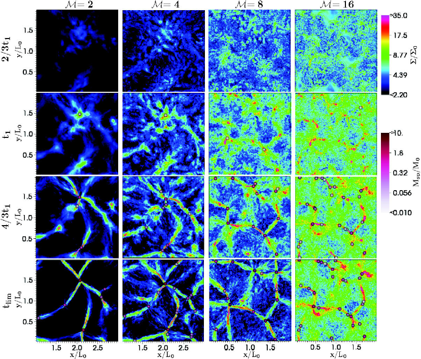
First, we provide an overview of the dynamical evolution in our models. Figure 1 shows the surface density evolution of different Mach numbers at , , , , where is the time for the first core to collapse in each simulation, corresponding to for . The dependence of on is discussed below.
The notable density structures seen in all models are filaments and cores. Also shown in Figure 1 are the locations of sink particles. Because gaseous filaments are unstable to longitudinal self-gravitating fragmentation (Nagasawa 1987), the suggestion has been that there is a two-stage process for core formation, with filaments first forming, and then fragmenting gravitationally (e.g., André et al. 2014). However, we find a subtly different progression. Figure 1 makes clear that cores and filaments develop simultaneously, rather than filaments forming first, followed by fragmentation into cores. Snapshots at closely-space time intervals show that the central densities of proto-cores and filaments grow together, until some of the gravitationally unstable cores collapse and form sink particles. As a result, the sink particles are not randomly distributed in the post-shock region, but are dotted along the long thin filamentary over-dense structures. Because our simulations do not include feedback to limit accretion, sink particles continually accrete surrounding material, and after some time may merge with one another.
The similarity in the density structure patterns of or arises because they have the same seeds for turbulence perturbations. Because of the planar converging flow geometry, the and component of the large scale velocity are not changed by the shock, and these velocities seed the density fluctuation patterns that grow to create filaments and cores. Thus, the structure provided by turbulence is crucial to initiation of the self-gravitating cores that collapse to make sinks. However, it is not true that the cores are formed simply from the growth of initial perturbations. Filaments and clumps can merge and fragment before they finally collapse into sink particles.
For the present simulations, the initial turbulent motions are generally subsonic. Although the structures that grow are seeded by the turbulent compression, self-gravity is crucial to their development444Even for the models with larger-amplitude turbulence, gravity is important for creating core-forming filaments.. This is true for both filaments and cores. We note, however, that on larger scales for which flow velocity would be supersonic, filamentary structures can form from turbulent compression alone. This sort of filament, for which gravity is not important, is distinct from the filaments formed in our simulations555André et al. (2010) discusses observations of filaments in both non-self-gravitating and self-gravitating clouds..
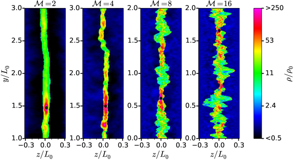
Figure 2 shows an slice through the density maximum at the time when collapse leads to the first sink particle. Evidently, the post-shock layer seen in cross section can be highly nonuniform, especially for and . This is due to nonlinear thin-shell instabilities of the post-shock layer (Vishniac 1994) that are stronger at higher Mach number. As a result of these instabilities, the gas is vertically dispersed and the density in the post-shock region is lower than , the value that would apply for a simple isothermal shock. The thickness of the post-shock layer is correspondingly higher than the value that would apply in the absence of instabilities. In fact, at later times, the median density (and pressure) of the post-shock region is nearly independent of Mach number. This leads to a very shallow dependence of core mass on Mach number, which is discussed further in §3.3. We note that magnetic fields reduce instabilities of the post-shock region (Chen & Ostriker 2014), so that the post-shock density and magnetic pressure increase with inflow Mach number.
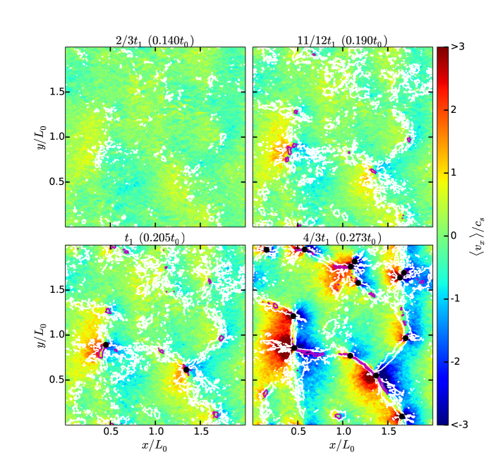
The map of at different times is shown in Figure 3. At the early core-building stage, the velocities are sub-sonic, converging towards the ridge of growing filaments (see also GO11, Chen & Ostriker 2014), due to the gravity from cores and filaments. After a core collapses to reach an LP profile, a sink particle is created and the surrounding material accretes onto the sink particle at the free-fall velocity.
3.1.2 Collapse of the First Cores: the Non-linear Time and Mass
Treating the post-shock layer as a slab with half thickness and surface density that grows in time, for linear-amplitude in-plane perturbations with , GO11 showed the wavelength of the unstable mode that would have the greatest exponential amplification at a given time is
| (19) |
where . The time at which an amplification is reached is
| (20) |
A characteristic mass associated with this mode is
| (21) |
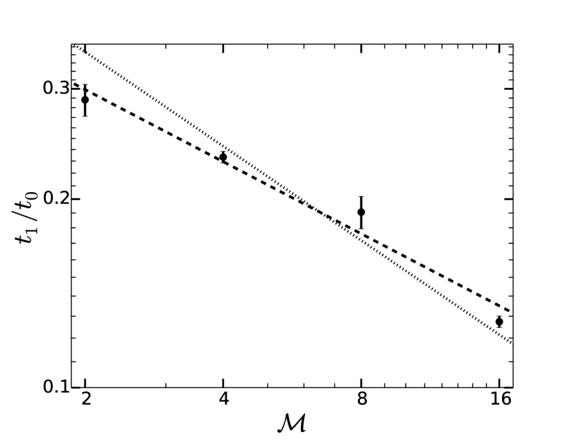
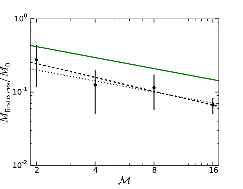
We fitted the time for the first core to collapse and the average mass of the first five cores in each simulation as a function of Mach number. In addition to the primary models (boldface in Table 2), we also included M02L4N1024, M04L4N1024, and M16L1.5N768 models, which have the same resolution and have been demonstrated to have sufficient box-size (see §3.2). The result is shown in Figure 4. Our fit gives and . The dependence of and on Mach number is similar to the dependence of Equations (20) and (21), and would give coefficients in Equations (20) and (21) comparable to our fits.
However, the large dispersion in (see Figure 4) suggests a process more complex than local growth of cores with in-plane waves . In particular, filament development with and unequal clearly plays a role in core formation. We note that using , Equation 19 gives , which we find is roughly equal to the typical filament separation seen in Figure 1, and also consistent with what was found in Van Loo et al. (2014). Thus, both the time to first collapse and the prominence of filaments implies that non-linear instability of asymmetric self-gravitating in-plane modes is important to core formation.
Finally, we note that the mass per unit length associated with the most amplified mode is , which is equal to twice the critical mass per unit length for an isothermal filament (Ostriker 1964), or for .666For a self-gravitating isothermal sheet with fixed surface density and scale height , the mass per unit length of the fastest growing mode is also . Of course, this mass is not all available at time , because only a fraction of this has been gathered into the filament. We find that typical values of the mass per unit length in filaments at time is .
3.1.3 Evolution of Cores
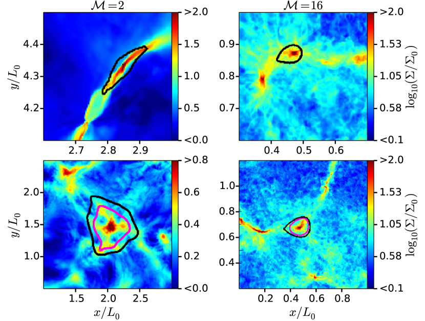
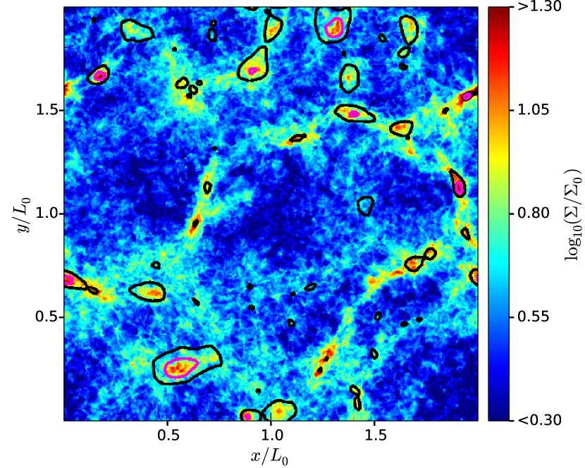
Examples of core finding for individual -cores and an overall map of all -cores in one simulation are shown in Figures 5 and 6. We can see clearly that cores are associated with filaments. A typical mass core is often found embedded in dense filaments. Although high mass cores may form in relative isolation early on, these locations often become junctions of filaments later on. These structures of cores lying in filaments or at the junctions are qualitatively very similar to the observation of star-forming regions with Herschel (André et al. 2014), as well as previous work (e.g., Johnstone & Bally 1999; Hartmann 2002).
GO09 classified the core development into four different stages: core building, core collapse, envelope infall, and late accretion. These stages can also be seen in our simulations, as illustrated in Figure 7 and 8 of the density (angle-averaged) and velocity profiles of typical cores. Initially at the core building stage, the core evolves in quasi hydrostatic equilibrium, with subsonic internal velocities. The core mass and density grow slowly as the gas from surrounding environment flows into the core potential well. When the core becomes gravitationally unstable, it collapses in a short timescale, reaching the LP profile. Then a sink particle is created in the core center, and starts accreting the gas from the envelope, causing the density to drop as the core collapses inside-out and approaches , a profile close to the expectation for free-fall (Shu 1977).
Noticeably, the angle-averaged core density profiles continue to drop smoothly beyond the effective core radius as shown in Figure 7 and 8. We note, however, this is partly due to the method we use to calculate , which takes the average density in a spherical shell at distance from the core center, including the low-density pre-shock gas at outside of the planer post-shock layer. For example, the density profile of the core in Figure 8 only extends to along some directions and is much less smooth than the angle-averaged density profile, as can be seen in the upper right of Figure 5. The anisotropy of cores (e.g., as in the upper left of Figure 5) can also make the angle-averaged density differ from the density profile along individual principal axes. Nevertheless, cores often extend beyond their effective radius , because they are formed in denser environments than the average post-shock density, and instantaneous tidal forces (which define ) do not limit the material that may ultimately fall into a sink particle. In fact, we often see that the mass of the sink continues to grow after it reaches the mass of the -core. There is no obvious boundary between the envelope infall and late accretion stages, as discussed in §3.4.1.
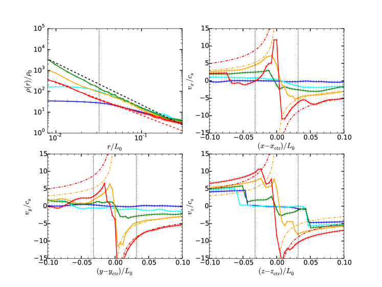
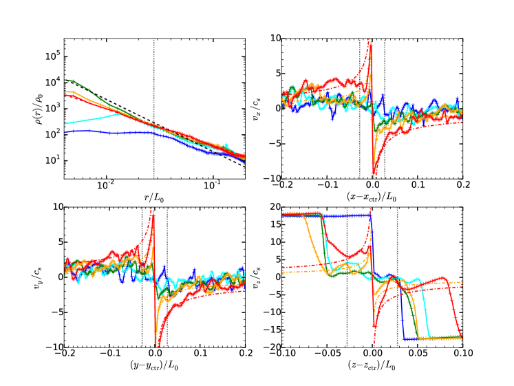
In our tests of the case with high-amplitude perturbations, the overall evolution is very similar to the low-amplitude cases. Cores and filaments still form in a similar manner, with cores embedded within filaments. At smaller scale (), both the initial velocity perturbation in Equation (9) is smaller and the turbulence dissipation timescale is shorter. As a result, even when the large-scale velocity perturbation is super-sonic, the high density regions within filaments where cores form are generally sub-sonic or trans-sonic, leading to very similar core evolution dominated by thermal pressure and gravity. Individual cores formed in simulations with high-amplitude velocity perturbations show the same internal collapse and infall profiles as shown in Figures 7 and 8.
3.2. Convergence of isothermal fragmentation
In order to understand protostar formation in our simulations, it is important to test numerical convergence, both to make sure the fragmentation process is not purely numerical, and the cores in our simulations are well resolved. In the literature, there has been a debate of whether fragmentation in isothermal HD simulations is determined by purely numerical rather than physical factors. If an isothermal sphere were to collapse homologously, the Jeans length within the sphere would decrease with radius as . This led to the early idea (Hoyle 1953) of hierarchical fragmentation into smaller pieces until pieces are no longer isothermal. In reality, however, core collapse is highly nonuniform and leads to centrally-concentrated structures (Bodenheimer & Sweigart 1968; Larson 1969; Penston 1969). At every radius in the asymptotic LP solution, the Jeans length is comparable to the radius. Thus it is not obvious that fragmentation can happen at arbitrarily small scales even for a simple isothermal equation of state. Martel et al. (2006) carried out a series of isothermal SPH simulations employing particle splitting techniques, and argued that the core masses they found are determined by numerical resolution and the density threshold of sink particles. However, the highest resolution they used only marginally resolves the Jeans mass at the density threshold for their sink particles, and they did not test with a higher resolution or density threshold. Krumholz (2014) further suggested that isothermal evolution with self-gravity cannot lead to a characteristic distribution of fragment mases, and that stellar masses must depend crucially on non-isothermal effects. However, Inutsuka & Miyama (1997) found that filaments (even with supercritical mass per unit length ) fragment longitudinally (rather than collapsing to a spindle) provided that the initial density perturbations are sufficiently large. In real clouds, as cores and filaments begin their growth together, filaments may not become supercritical until after cores have become nonlinear.
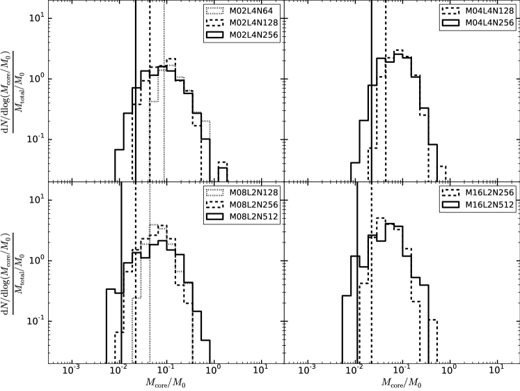
We find that at the stage of core collapse, there is in fact a well defined characteristic mass scale for the ideal isothermal case. Figure 9 shows the core mass function (CMF) for -cores of models with different resolutions for each Mach number. For the lower resolution models, the distribution of core mass drops off rapidly at . This shows that cores with zones may not be well resolved. However, as we increase the resolution, although the CMF continues to extend towards lower masses, the peak of the CMF does not vary much (see also Table 3). We note that the density threshold for sink particle creation also increases with resolution as described in Equation (8). For the highest resolution model of each Mach number, the CMF peaks at a mass of cores that are well resolved with . Although simulations with even higher resolutions could show a modification of the CMF, especially at the low mass end, our models suggest that the CMF peak, or the characteristic mass of the core, would remain the same.
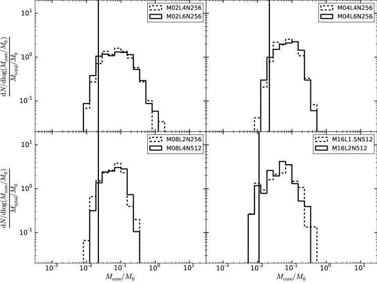
We also investigated the numerical effect of horizontal box size in our simulation. The box size limits the longest wavelength perturbation that can grow in the simulation domain , and also limits the amplitude of initial velocity perturbations as described in Equation (10). Figure 10 shows histograms of of models with different box sizes. The distributions of do not vary appreciably with increasing box size in our models (see also Table 3). This shows that for our simulations with a box sufficiently larger than the dominant non-linear wavelength (, see Equation 19), the box size does not have a significant effect on core formation.
Although our simulations show a well-defined, converged value for the peak in the distribution of core masses at the point of singularity formation, fragmentation at later stages could in principle further alter this distribution. In particular, infall of rotating envelopes leads to formation of prestellar accretion disks, which we do not model in the current study. These accretion disks would be susceptible to fragmentation if external and internal heating are not properly taken into account. We conclude that it is important to distinguish between the core stage and subsequent stages in assessing the outcome of self-gravitating fragmentation in turbulent clouds. Going from the CMF to IMF physically involves structures at increasingly high temperature, and simulations must include these non-isothermal effects to model the stages of disk formation and evolution.
3.3. Core Properties
3.3.1 Typical Core Mass, Radius, and Density
We summarise the basic physical properties for -cores and -cores of different models in Table 3 and Table 4. Cores containing fewer than 27 grid cells are considered to be poorly resolved (similar to the resolution limit in Figure 9) and are not included in Table 3 or further analysis. Table 3 again shows the convergence of the characteristic mass for simulations with different resolutions and box sizes, as discussed in §3.2.
The median -core sizes and masses are quite similar for different Mach numbers, as a result of the similar post-shock density across different Mach numbers . Using the fiducial values of and from Table 1, the characteristic core masses and radii are and pc. Figure 11 plots the mass defined by gravitational potential alone of -cores () versus the post shock critical Bonner-Ebert sphere mass () and Mach number (. Setting in Equation (1), the critical Bonner-Ebert mass becomes
| (22) |
We fit the post-shock density field (defined as zones with ) with a log-normal distribution with mean value of equal to and dispersion . This distribution remains roughly constant over the time of core formation. We then used and at the time when the core formation rate is roughly at its peak to estimate the corresponding distribution of : from Equation (22), also follows a log-normal distribution with a mean value and dispersion , which is plotted as dots and error bars on the x-axis in Figure 11. On the y-axis of Figure 11, we plot the median value of and error bar showing the median absolute deviation of in logarithm space, as listed in Table 3. Typically , consistent with the general range expected for isothermal fragmentation. The median core mass depends on inflow Mach number as . As noted above, the weak variation in , and resulting weak dependence of the characteristic mass on , is a result of instability of the post-shock layer. In magnetized simulations, for which these instabilities are suppressed, the post-shock density is close to the expectation of magnetized isothermal shock . Combining this effect with anisotropic flows along magnetic field lines leads to a stronger dependence of core mass on Mach number close to (Chen & Ostriker 2015, in preparation).
With increasing Mach number, we find that more cores form per unit area in each simulation run. Our fitting gives for -cores, similar to what would be expected from the decreasing separation of filaments of Equation (19).
In comparison to the -cores, the -cores show a wider range of physical properties. This can be explained by the fact that they include cores at very different evolutionary stages, as discussed in detail in the following sections. The median masses of cores are lower, and median radii are higher, for -cores compared to cores. The properties of -cores also show a stronger dependence on Mach number, because they represent the non-linear size and mass in the post-shock sheet that scales as (see Equation (19) and (21)), as also shown in the earlier studies by GO11.
| Model | aafootnotemark: | aafootnotemark: | a,ba,bfootnotemark: | ccfootnotemark: | |
|---|---|---|---|---|---|
| M02L6N256 | 267 | 2.47 | |||
| M02L4N256 | 239 | 2.49 | |||
| M02L4N128 | 169 | 2.64 | |||
| M02L4N64 | 220 | 1.72 | |||
| M04L6N256 | 346 | 4.81 | |||
| M04L4N256 | 266 | 5.54 | |||
| M04L4N128 | 264 | 5.50 | |||
| M08L2N512 | 232 | 7.25 | |||
| M08L2N256 | 197 | 8.21 | |||
| M08L2N128 | 182 | 9.10 | |||
| M08L4N256 | 121 | 7.56 | |||
| M16L2N512 | 122 | 7.62 | |||
| M16L1.5N512 | 107 | 7.93 | |||
| M16L2N256 | 158 | 13.17 |
| Model | |||||
|---|---|---|---|---|---|
| M02L6N256 | 94 | 0.87 | |||
| M02L4N256 | 86 | 0.90 | |||
| M04L6N256 | 151 | 2.10 | |||
| M04L4N256 | 103 | 2.15 | |||
| M08L2N512 | 139 | 4.34 | |||
| M16L2N512 | 103 | 6.44 | |||
| M16L1.5N512 | 83 | 6.15 |
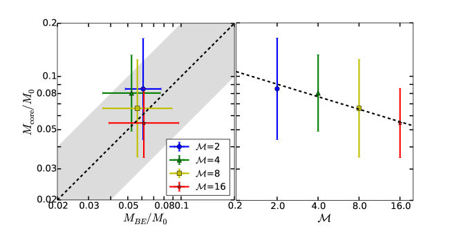
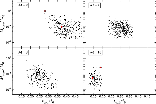
Figure 12 plots the mass and time of collapse for every -core. For higher Mach numbers, the cores form sooner and in a less extended period of time, as explained in §3.1.2. This also leads to more similarity between and cores (see Table 3 and 4) for higher Mach numbers. There is a similar pattern in models with different . The average core mass decreases slightly with time, as smaller cores form in dense filaments which become more developed at later times. At the end of each simulation, the core formation rate drops, when most material in the post-shock region has been accreted by the sink particles. This is further discussed in §3.4.2.
The median value and the median absolute deviation at a logarithm scale of core mass and radius in high-amplitude velocity perturbation simulations are and . This is about % of the core mass and radius in low-amplitude perturbation cases (see the M08L2N256 model in Table 3), but subject to the limited statistics of 21 cores. There are also a few massive turbulence supported cores formed in high-amplitude simulations, which are not seen in low-amplitude cases; this is further discussed in the last paragraph of §3.3.4
3.3.2 Core Binding
Since the -cores are identified at the time of collapse by definition, they are expected to have density profiles close to the LP profile. This is indeed the case, as shown below (see also Figure 7 and 8). Integrating Equation (2), the mass of the core will be proportional to its radius
| (23) |
Solving the Poisson equation
| (24) |
the gravitational potential of an isolated core with LP profile can be written as
| (25) |
where is the gravitational potential at the edge of the core, . Using for the definition of bound cores, we can obtain the relationship of and :
| (26) |
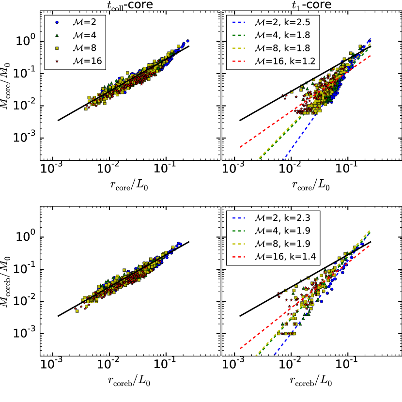
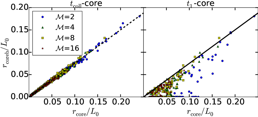
The left panels of Figure 13 shows the mass-radius relation of the -cores defined by gravitational potential alone and the bound -cores with . The results are consistent with equation (23), i.e. and , showing that essentially all cores approach the LP density profile at the time of collapse. The left panel of Figure 14 plots the size of every -core defined by gravitational potential alone compared to the corresponding bound core with , showing that , as expected from Equation (26). Due to the potential of surrounding cores and filaments, gravitational potential profiles at the edges of the -cores in the simulations are slightly flatter than that they would be for isolated cores. Therefore, we find , slightly smaller than the coefficient in Equation (26).
In comparison, many -cores are not strongly centrally concentrated or gravitationally bound, as shown in the right panels of Figure 13 and Figure 14. The mass radius relation of -cores is found to be with , implying that they have flatter density profiles than the LP profile or critical Bonner-Ebert sphere. This is consistent with results for -cores in previous simulations with or without magnetic fields (Gong & Ostriker 2009; Chen & Ostriker 2014), and similar to many core-property surveys in different molecular clouds (e.g., Curtis & Richer 2010; Kirk et al. 2013), in which with various tracers (see Figure 7 and corresponding discussions in Kirk et al. (2013)). This suggests that cores identified at any given time in simulations or observations (-cores in our case) can be in very different stages of evolution. Because any individual core spends most of its lifetime in the core building stage, many of the cores in a given snapshot of time will resemble sub-critical Bonner-Ebert spheres777Cores at very early building stages would, however, be difficult to pick out in a noisy background, as the density contrast would be low., with only a fraction of them more evolved and in the core collapse stage. Some of the cores we identify, especially low mass cores, are structures with weak self-gravity and may not finally collapse. The spread of mass-radius relation is larger for lower mass cores in the right panels of Figure 13, implying a wider range of evolutionary stages. Interestingly, we find a shallower mass-radius relation at for higher Mach number simulations, indicating those cores are more evolved and therefore more centrally concentrated. With complete population studies from Herschel and ALMA that are able to quantify the relative populations of strongly concentrated cores versus those with flatter density profiles, the timescales for core collapse versus core building stages can be measured (see Marsh et al. (2014) for initial Herschel results).
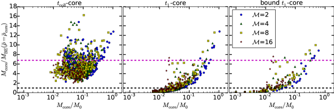
Another way to quantify whether a core is gravitationally unstable or not is to look at the ratio of core mass to the critical Bonner-Ebert sphere with the same average density of the core. For the LP density profile, the ratio (see Equation (1)). In Figure 15, all -cores are gravitationally unstable, with the ratio . In comparison, among all the -cores , only of cores defined by the gravitational potential alone, and of bound cores with , are gravitationally unstable with . There is also a clear trend that this ratio increases with mass, which is not present for the -cores. This again suggests that many -cores, especially the low mass ones ( in the middle and right panels of Figure 15), are transient structures from turbulence perturbations, and may not finally give rise to star formation. This is also evident in the CMF described in §3.3.4.
The core binding properties in high-amplitude perturbation simulations are similar to the low-amplitude cases as discussed above. All of the -cores are strongly gravitationally bound, whereas most of the -cores, especially the lower mass ones, are not strongly concentrated or highly stratified.
3.3.3 Core Shape
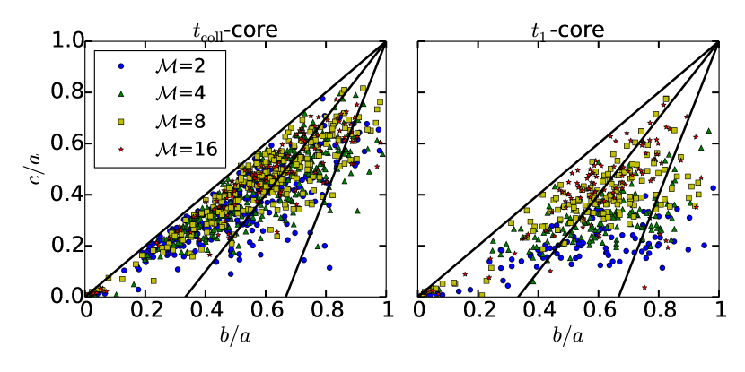
The shape of a core can be described by the eigenvalues of the moment of inertia tensor (e.g., Gammie et al. 2003; Nakamura & Li 2008)), or the covariance matrix of offsets with respect to the center of mass (GO11). Let a,b and c be the lengths of the principal axes and . A prolate core has , and an oblate core . The core aspect ratio distribution in Figure 16 shows several interesting features. First, most cores are prolate and triaxial, and only a small fraction are oblate. If cores form via fragmentation in isothermal filaments, they are expected to be initially prolate, since the fragmentation scale along filaments is expected to have separations larger than the filament diameter (Nagasawa 1987; Inutsuka & Miyama 1992). In fact, the typical -core aspect ratios are smaller than the ratio of spacing to diameter for the fastest growing mode of filament fragmentation, again suggesting that cores are not exclusively formed as instabilities in filaments. Second, the fraction of cores that are prolate is higher in -cores than -cores, implying more evolved cores tends to be more prolate, whereas cores formed via gravitational instability of filaments become more spherical in time. Last, among all -cores, more are prolate for higher Mach numbers, consistent with those cores in high Mach number simulations being slightly more evolved, as also indicated in the left panels of Figure 13.
3.3.4 Core Mass Function
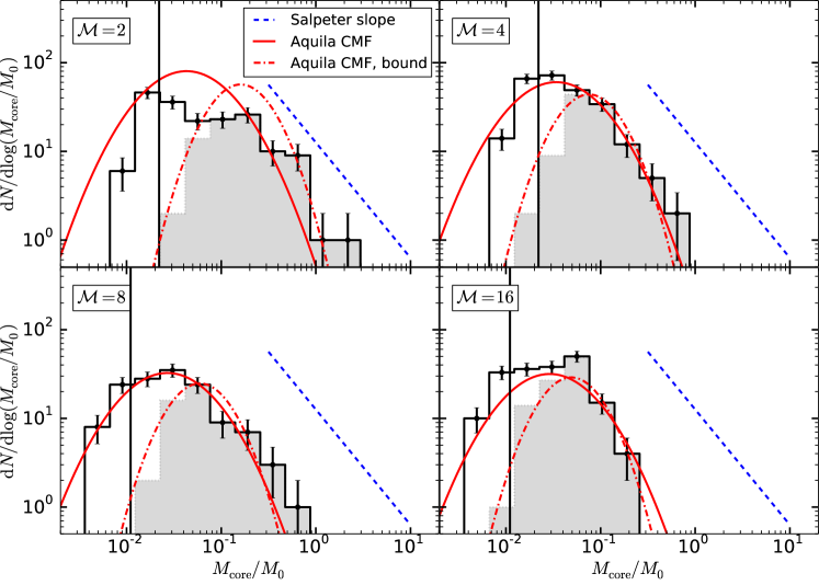
The core mass functions (CMFs) of -cores are shown in Figure 17. To compare the CMFs from our simulations to the observed CMF,we match the median mass, and only compare the shape of different distributions with a logarithmic horizontal scale. This is because the mass scale in our simulations can be adjusted by changing (see Equation (12)). Figure 17 includes the (shifted) fit to full Aquila core sample of André et al. (2010), and the (shifted) fit to the gravitationally bound portion (Könyves et al. 2010). Although our statistics are limited for high-mass cores, for reference in Figure 17 we also show the slope of the Salpeter mass function .
The CMF of the full sample of -cores in Figure 17 is similar to the shape of the observed CMF near the peak. Among the -cores, the majority of the small cores are weakly self-gravitating transient structures. If we only include the gravitationally bound -cores (shaded histogram in Figure 17), the distribution is similar to the gravitationally bound cores observed in Aquila (Könyves et al. 2010). Although statistics for our simulations (and observed) cores are too poor to fit a high-end mass slope with confidence, the distribution of high-mass -cores appear to be consistent with the log-normal fit of observed cores, and shows no evidence of an extended power-law tail.
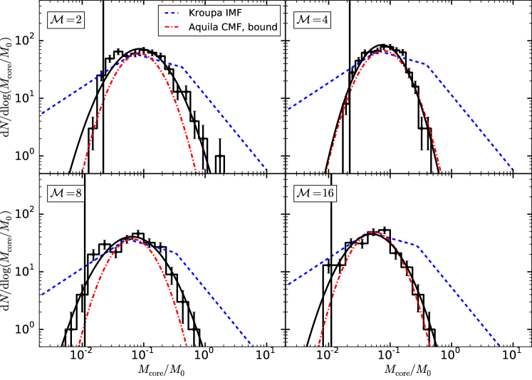
Figure 18 shows the mass distribution of -cores. We also show, for each model, a log-normal fit to the distribution. In addition, Figure 18 includes for comparison the bound core Aquila fit and the Kroupa IMF (shifted so that median masses match). As can be seen in Figure 18, the CMFs of -cores show a statistically significant ( in the high mass bins) deficit of high mass cores compared to the shape of the observed IMF, and can be well-fitted by relatively narrow log-normal distributions with standard deviations of . This is simliar to the bound core CMF log-normal fit in the Aquila cloud, which has a standard deviation .
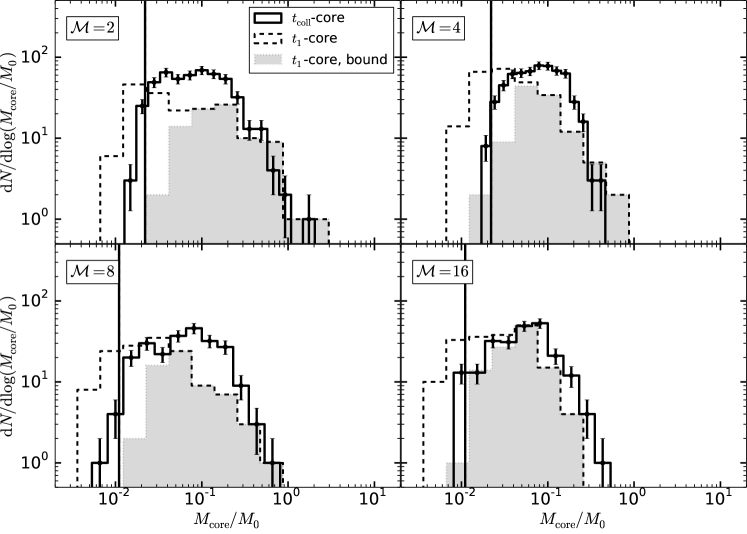
Figure 19 shows a comparison between the -cores and the -cores, for each value of . It is interesting that the CMFs of -cores and -cores do not match in our simulations. The -cores show a wider distribution with more low-mass cores, and the characteristic core mass is a factor of smaller than that of -cores. However, the bound portion of the -core distribution is more similar to the -cores.
The differences between -cores and -cores has interesting implications for interpreting observations. Observations of CMFs represent a snapshot in time of GMCs, and often do not distinguish between gravitationally stable (weakly bound) or unstable (strongly bound) cores (e.g., Nutter & Ward-Thompson 2007; André et al. 2010). Our results suggest that if the cores defined in observations are comparable to our -cores, then a large fraction of the low mass cores in observed CMFs may not end up collapsing, or gain a significant fraction of mass before they collapse. This also implies that the observed similarities between the CMF and IMF cannot be simply interpreted as a fundamental correlation between stellar mass and core mass, with each core contributing the same proportion of its mass to the final star, because we know that there is not a one-to-one mapping between cores observed at a given instant and cores at the time of collapse of star formation. However, the similarity between our bound -cores and our -cores suggests that an analogous selection of just gravitationally bound cores can be obtained in observations, to probe the CMFs that better represent the initial mass reservoir for star formation.
The difference between the CMFs of -cores in our models and the observed IMF could have several possible reasons. First, the idealizations or physics in our simulations may be unfavorable for high mass core formation. For example, the presence of magnetic field, or a larger amplitude turbulent velocities might be able to provide additional magnetic or turbulence support, encouraging high mass core formation888However, the magnetized simulations of Chen & Ostriker (2014) show no difference in median core masses from unmagnetized models. Indeed, in our high-amplitude perturbation tests, 3 among the 21 cores are very massive with . These high-mass cores are all turbulent supported with (most of the smaller cores have ). This is suggestive that massive turbulent supported cores may be more prevalent in systems with high velocity dispersion, but a more systematic study using global rather than local models is required.
Alternatively, the final mass of a star may not be directly set by the mass of the associated -core. For example, more massive cores may be able to hold onto a larger fraction of their -core mass, or capture more mass via competitive accretion at late times from the mutual reservoir. Those factors cannot be directly assessed in our simulations, since the sink particles are artificially merged, and feedback processes are not included. However, there is some evidence that the sink particles in higher mass cores accrete faster, which is discussed in §3.4.1.
3.4. Sink Particles
3.4.1 Accretion Rates of Sink Particles
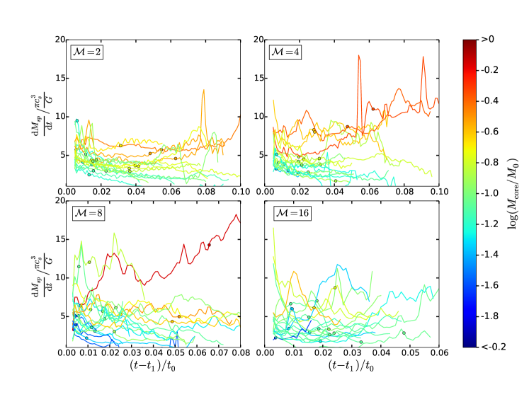
When a sink particle is created, gravity dominates over gas pressure in the envelope, and the gas accelerates into the sink, approaching free-fall. A spherical LP density profile with gas free-falling to the center would have a constant mass accretion rate999The accretion rate unit, , is equal to , for km/s.:
| (27) |
In fact, pressure reduces the accretion rate somewhat (see below), but infall still progresses from the inside to the outside of the envelope. After this inside-out collapse reaches out to where the density profile flattens out and there is more turbulent and thermal support, the accretion rate is expected to change. Figure 20 illustrates the accretion history of sink particles. On average, the accretion rate remains roughly constant, with a slight rising trend after the sink mass equals the -core mass. However, we see no clear separation between the accretion of the initial tidally-bound core and later stages; this is not surprising, as the angle-averaged density profile is continuous at the effective core radius. Noticeably, there are outbursts in accretion rates with the peak several times higher than the average for a period of . This is due to the clumpy density structures that develop and fall into the sink. In reality, the infall onto the protostar has to be processed through an accretion disk which is not resolved in our simulations. The additional mass falling into the star during outbursts of this kind may trigger gravitational or magnetic instabilities in the inner disk, leading to more dramatic outbursts in YSOs, for instance, the episodic accretion of FU Ori-type stars (Audard et al. 2014; Ohtani et al. 2014).
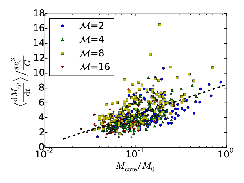
Figure 20 also shows a trend that the average accretion rate increases with the corresponding -core mass, which is quantified in Figure 21. The average depends linearly on , but there is also a big dispersion with a factor of in accretion rates at a given core mass. Another way to show the dependence of accretion rate on core mass is to look at the mass of sink particle at the free-fall timescale of the core. Figure 22 shows sink particle masses at 1, 2, and 4 times the initial free-fall time of the -cores. The initial mass in the core is accreted by the sink at , after which the accretion rate drops for low mass cores while it rises for high mass ones. At , the ratio of sink mass to -core mass is a factor of larger for the highest mass cores than the lowest mass ones. This trend provides one possible explanation of the discrepancy between the CMF in our simulations and the observed IMF, although in addition to this effect, the final stellar mass would depend on feedback and mass loss at later stages of star formation, which is beyond the scope of this paper.
The sink particle accretion properties of our high-amplitude velocity perturbation simulations are similar to the low-amplitude cases discussed above.
3.4.2 Star Formation Rate
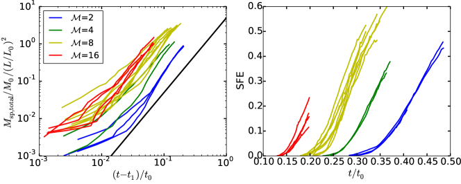
The total mass in sink particles, as shown in the left panel of Figure 23, increases super-linearly with time, roughly as . This is because both the mass of individual sinks and the total number of sink particles increases linearly with time. Lee et al. (2014) also obtained a similar result that the accreted mass grows as in turbulent MHD simulations. For higher Mach numbers, we find that there is more mass accreted at a given time, both because sink particles form faster, and more sinks form per unit area. We note that this only represents the early stage of star formation when gravity dominates, and the surrounding gas is abundant. The star formation rate would have to drop at a later times when stellar feedback becomes important and gas in the GMC is exhausted or removed.
The star formation efficiency (SFE) is shown in the right panel of Figure 23. The SFE is defined as the ratio of total mass in all sinks to , the total mass that has entered the box (or the shocked gas). As the mass in sinks grows , the SFE increases linearly with . Similar to all simulations without feedback (eg. Lee et al. (2014); Smith et al. (2009)), gas is accreted on the free-fall timescale, resulting in a high SFE of .
4. Summary
In this work, we have used three-dimensional numerical simulations to explore the physics of pre-stellar core formation and the subsequent core collapse that leads to the formation of protostars. We focus on local regions (pc) within GMCs where a supersonic turbulent flow converges, triggering star formation in the post-shock layer. Our simulations adopt an idealized isothermal equation of state, include gravity from both gas and sink particles, and explore a wide range of Mach numbers () for the inflow gas. We terminate our simulations at late times, when most of the gas in the post-shock region has been accreted by the sink particles.
For a fixed Mach number, we have carried out a series of simulations with different resolutions and box sizes to study potential numerical effects, especially the convergence of isothermal fragmentation. We have obtained the properties of cores in each model, for both cores identified at the time of individual collapse (-cores) and from a snapshot at the time of first singularity formation in each simulation (-cores). We study the statistical properties of cores, and compare the CMFs in our simulations to the observed CMF and IMF. In addition, we trace the mass accretion rate of sink particles, and its dependence on the core mass.
Our main conclusions are as follows:
-
1.
Cores and self-gravitating filaments form and evolve at the same time. Isothermal filaments do not collapse to become singular spindles (cf. Inutsuka & Miyama 1992, 1997) because both small-scale and large-scale over-densities are seeded by compression from turbulence, and filaments and cores grow simultaneously.
-
2.
At the time of singularity formation, all -cores approach the Larson-Penston asymptotic solution, giving a mass-radius relation of (see Figure 13), with the LP density profile extending beyond several times the angle-averaged tidal radius of the cores. Most -cores are prolate, consistent with filament fragmentation. The mass-radius relation of cores implies a flatter density profile with , similar to observations (e.g., Curtis & Richer 2010; Kirk et al. 2013). Many -cores are only weakly bound.
-
3.
At the stage of core collapse, there is a well-defined characteristic mass scale for fragmentation in our turbulent, self-gravitating simulations. The characteristic -core mass in our simulations converges as we increase the resolution and density threshold for sink particle creation. This mass is very close to the mass of a critical Bonner-Ebert sphere (see Equation (1)), taking the “edge” as equal to the mean pressure in the post-shock layer formed by the converging flow (See Figure 11).
-
4.
The characteristic core mass for the present simulations is insensitive to the Mach number of the large-scale converging flow. As the inflow Mach number increases, the post-shock density and pressure do not vary much, due to instabilities that disperse the gas in the post-shock layer, leading to similar core properties across different Mach numbers. For all models, the characteristic core mass is . We note, however, that inclusion of magnetic fields reduces these instabilities, such that the (magnetically-dominated) post-shock pressure is higher, and characteristic core mass is lower in models with higher Mach numbers (Chen & Ostriker 2015, in preparation)101010However, in the magnetized case, the characteristic core mass is still comparable to the critical Bonner-Ebert mass at the mean post-shock pressure.
-
5.
The CMFs of -cores in our simulations show a log-normal distribution with standard deviation (Figure 18). This is similar to the bound core distribution width for Aquila (Könyves et al. 2010). There is a significant deficit of high mass cores () compared to the shape of the observed IMF. However, the CMFs of -cores (Figure 17) show a wider distribution with more low mass cores, similar to the shape of the full observed CMF (e.g., Alves et al. 2007; Nutter & Ward-Thompson 2007; André et al. 2010). This suggests that observed CMFs, similar to our -cores, may include cores at an early stage of evolution that will gain a significant amount of mass before collapsing, or transient structures from turbulence perturbations that may never collapse. Therefore, the observed CMF from a cloud “snapshot” may not represent the distribution of mass reservoirs for protostar collapse. We find, however, that the -cores that exceed the critical BE mass have a distribution that is closer to that of the -cores; a similar selection could be made for observed cores.
-
6.
The mass accretion rate of sink particles increases weakly with the corresponding -core mass (Figure 22), suggesting that competitive accretion may play a role in filling out the high-mass portion of the IMF. Individual sink particles accrete at roughly constant , and continue to gain more mass even after they have exceeded the mass of the core when it first collapsed. There are outbursts in (Figures 20, 21) due to clumpy density structures forming and falling into the sink.
-
7.
The star formation rate (measured as the total mass in sink particles) in each converging-flow simulation increases with time as , as both the formation rate of sink particles (i.e., rate of cores surpassing the collapse threshold), and the accretion rate of individual sinks are roughly constant. This result is similar to the “accelerating star formation” found in some other recent simulations (Lee et al. 2014). For a realistic cloud, however, the duration of any given large-scale converging flow would be less than the crossing time of the cloud, and feedback would limit the accretion within any individual core.
The present suite of models extend previous simulation studies of gravoturbulent fragmentation in several important ways. Most notably, by systematically varying the Mach number, we are able to test the influence of a key environmental parameter, and by systematically varying the resolution, we are able to demonstrate that evolution robustly includes a core-collapse stage with well-defined mass. The physical ingredients of our simulations are limited, however, in particular lacking magnetic fields, feedback from forming stars, and effects of environmental evolution. Furthermore, global cloud simulations are required in order to incorporate the full spectrum of turbulence at realistic amplitudes. Other work currently underway will address these limitations while maintaining a focus on systematic surveys of the environmental parameter space.
References
- Alves et al. (2007) Alves, J., Lombardi, M., & Lada, C. J. 2007, A&A, 462, L17
- André et al. (2009) André, P., Basu, S., & Inutsuka, S. 2009, The formation and evolution of prestellar cores, ed. G. Chabrier (Cambridge University Press), 254
- André et al. (2014) André, P., Di Francesco, J., Ward-Thompson, D., et al. 2014, Protostars and Planets VI, 27
- André et al. (2010) André, P., Men’shchikov, A., Bontemps, S., et al. 2010, A&A, 518, L102
- Audard et al. (2014) Audard, M., Ábrahám, P., Dunham, M. M., et al. 2014, ArXiv e-prints, arXiv:1401.3368
- Ballesteros-Paredes et al. (2007) Ballesteros-Paredes, J., Klessen, R. S., Mac Low, M.-M., & Vazquez-Semadeni, E. 2007, Protostars and Planets V, 63
- Bate (2009) Bate, M. R. 2009, MNRAS, 392, 1363
- Bate et al. (1995) Bate, M. R., Bonnell, I. A., & Price, N. M. 1995, MNRAS, 277, 362
- Bodenheimer & Sweigart (1968) Bodenheimer, P., & Sweigart, A. 1968, ApJ, 152, 515
- Bonnor (1956) Bonnor, W. B. 1956, MNRAS, 116, 351
- Chen & Ostriker (2012) Chen, C.-Y., & Ostriker, E. C. 2012, ApJ, 744, 124
- Chen & Ostriker (2014) —. 2014, ApJ, 785, 69
- Curtis & Richer (2010) Curtis, E. I., & Richer, J. S. 2010, MNRAS, 402, 603
- di Francesco et al. (2007) di Francesco, J., Evans, II, N. J., Caselli, P., et al. 2007, Protostars and Planets V, 17
- Dobbs et al. (2014) Dobbs, C. L., Krumholz, M. R., Ballesteros-Paredes, J., et al. 2014, Protostars and Planets VI, 3
- Ebert (1955) Ebert, R. 1955, ZAp, 37, 217
- Federrath et al. (2010) Federrath, C., Banerjee, R., Clark, P. C., & Klessen, R. S. 2010, ApJ, 713, 269
- Gammie et al. (2003) Gammie, C. F., Lin, Y.-T., Stone, J. M., & Ostriker, E. C. 2003, ApJ, 592, 203
- Gong & Ostriker (2009) Gong, H., & Ostriker, E. C. 2009, ApJ, 699, 230
- Gong & Ostriker (2011) —. 2011, ApJ, 729, 120
- Gong & Ostriker (2013) —. 2013, ApJS, 204, 8
- Hartmann (2002) Hartmann, L. 2002, ApJ, 578, 914
- Hockney & Eastwood (1981) Hockney, R. W., & Eastwood, J. W. 1981, Computer Simulation Using Particles
- Hoyle (1953) Hoyle, F. 1953, ApJ, 118, 513
- Hunter (1977) Hunter, C. 1977, ApJ, 218, 834
- Inutsuka & Miyama (1992) Inutsuka, S.-I., & Miyama, S. M. 1992, ApJ, 388, 392
- Inutsuka & Miyama (1997) Inutsuka, S.-i., & Miyama, S. M. 1997, ApJ, 480, 681
- Johnstone & Bally (1999) Johnstone, D., & Bally, J. 1999, ApJ, 510, L49
- Kirk et al. (2013) Kirk, J. M., Ward-Thompson, D., Palmeirim, P., et al. 2013, MNRAS, 432, 1424
- Könyves et al. (2010) Könyves, V., André, P., Men’shchikov, A., et al. 2010, A&A, 518, L106
- Koyama & Ostriker (2009) Koyama, H., & Ostriker, E. C. 2009, ApJ, 693, 1316
- Kroupa (2001) Kroupa, P. 2001, MNRAS, astro-ph/0009005
- Krumholz (2014) Krumholz, M. R. 2014, ArXiv e-prints, arXiv:1402.0867
- Krumholz et al. (2004) Krumholz, M. R., McKee, C. F., & Klein, R. I. 2004, ApJ, 611, 399
- Kudoh & Basu (2008) Kudoh, T., & Basu, S. 2008, ApJ, 679, L97
- Kudoh & Basu (2011) —. 2011, ApJ, 728, 123
- Lada et al. (2008) Lada, C. J., Muench, A. A., Rathborne, J., Alves, J. F., & Lombardi, M. 2008, ApJ, 672, 410
- Larson (1969) Larson, R. B. 1969, MNRAS, 145, 271
- Lee et al. (2014) Lee, E. J., Chang, P., & Murray, N. 2014, ArXiv e-prints, arXiv:1406.4148
- Marsh et al. (2014) Marsh, K. A., Griffin, M. J., Palmeirim, P., et al. 2014, MNRAS, 439, 3683
- Martel et al. (2006) Martel, H., Evans, II, N. J., & Shapiro, P. R. 2006, ApJS, 163, 122
- McKee & Ostriker (2007) McKee, C. F., & Ostriker, E. C. 2007, ARA&A, 45, 565
- Men’shchikov et al. (2010) Men’shchikov, A., André, P., Didelon, P., et al. 2010, A&A, 518, L103
- Molinari et al. (2010) Molinari, S., Swinyard, B., Bally, J., et al. 2010, A&A, 518, L100
- Nagasawa (1987) Nagasawa, M. 1987, Progress of Theoretical Physics, 77, 635
- Nakamura & Li (2005) Nakamura, F., & Li, Z.-Y. 2005, ApJ, 631, 411
- Nakamura & Li (2008) —. 2008, ApJ, 687, 354
- Nutter & Ward-Thompson (2007) Nutter, D., & Ward-Thompson, D. 2007, MNRAS, 374, 1413
- Offner et al. (2014) Offner, S. S. R., Clark, P. C., Hennebelle, P., et al. 2014, Protostars and Planets VI, 53
- Ohtani et al. (2014) Ohtani, T., Kimura, S. S., Tsuribe, T., & Vorobyov, E. I. 2014, ArXiv e-prints, arXiv:1408.5596
- Ostriker (1964) Ostriker, J. 1964, ApJ, 140, 1056
- Padoan & Nordlund (2011) Padoan, P., & Nordlund, Å. 2011, ApJ, 730, 40
- Penston (1969) Penston, M. V. 1969, MNRAS, 144, 425
- Roy et al. (2014) Roy, A., André, P., Palmeirim, P., et al. 2014, A&A, 562, A138
- Schisano et al. (2014) Schisano, E., Rygl, K. L. J., Molinari, S., et al. 2014, ApJ, 791, 27
- Shu (1977) Shu, F. H. 1977, ApJ, 214, 488
- Shu et al. (1987) Shu, F. H., Adams, F. C., & Lizano, S. 1987, ARA&A, 25, 23
- Smith et al. (2009) Smith, R. J., Clark, P. C., & Bonnell, I. A. 2009, MNRAS, 396, 830
- Stone & Gardiner (2009) Stone, J. M., & Gardiner, T. 2009, New A, 14, 139
- Stone et al. (2008) Stone, J. M., Gardiner, T. A., Teuben, P., Hawley, J. F., & Simon, J. B. 2008, ApJS, 178, 137
- Stutzki & Guesten (1990) Stutzki, J., & Guesten, R. 1990, ApJ, 356, 513
- Truelove et al. (1997) Truelove, J. K., Klein, R. I., McKee, C. F., et al. 1997, ApJ, 489, L179
- Van Loo et al. (2014) Van Loo, S., Keto, E., & Zhang, Q. 2014, ApJ, 789, 37
- Vishniac (1994) Vishniac, E. T. 1994, ApJ, 428, 186
- Williams et al. (1994) Williams, J. P., de Geus, E. J., & Blitz, L. 1994, ApJ, 428, 693