Geometric Biases in Power-Spectrum Measurements

Abstract

The observed distribution of galaxies has local transverse isotropy around the line-of-sight (LOS) with respect to the observer. The difference in the statistical clustering signal along and across the line-of-sight encodes important information about the geometry of the Universe, its expansion rate and the rate of growth of structure within it. Because the LOS varies across a survey, the standard Fast Fourier Transform (FFT) based methods of measuring the Anisotropic Power-Spectrum (APS) cannot be used for surveys with wide observational footprint, other than to measure the monopole moment. We derive a simple analytic formula to quantify the bias for higher-order Legendre moments and we demonstrate that it is scale independent for a simple survey model, and depends only on the observed area. We derive a similar numerical correction formula for recently proposed alternative estimators of the APS that are based on summing over galaxies rather than using an FFT, and can therefore incorporate a varying LOS. We demonstrate that their bias depends on scale but not on the observed area. For a quadrupole the bias is always less than 1 per cent for $k>0.01h\,\mathrm{Mpc}^{\text{{-}}1}$ at $z>0.32$. For a hexadecapole the bias is below 5 per cent for $k>0.05h\,\mathrm{Mpc}^{\text{{-}}1}$ at $z>0.32$.

1 Introduction

The three-dimensional Power Spectrum (PS) of galaxies is one of the most important measurements that can be made from galaxy surveys. The Baryon Acoustic Oscillation feature in the PS can be used to obtain sub percent constraints on the expansion history of the Universe; The Redshift-Space Distortions (RSD; Kaiser, 1987) allow precise measurements of the growth rate of structure; And the Alcock-Paczynski (AP; Alcock & Paczynski, 1979) effect constraints very tightly the geometry of the Universe (for the most recent measurements see, e.g. Anderson et al., 2014; Samushia et al., 2014).

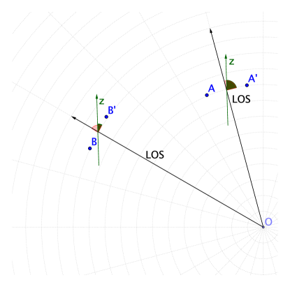
Both RSD and AP are imprinted into galaxy distribution as a signature along the line-of-sight (LOS) from the observer. To extract these signals in an unbiased way it is important that we analyse the data using the correct LOS that varies from a galaxy-pair to a galaxy-pair. It is geometrically impossible to define a Cartesian coordinate grid in such a way that the $\widehat{\bm{z}}$-axis is everywhere aligned with the LOS direction. Thus, the APS cannot be measured in Cartesian coordinates with one of the directions in dual Fourier space identified with the LOS.

Because the PS is a 2-point statistic, it relies on the properties of pairs of overdensities, although estimation methods can instead be based on pairs of galaxies. The varying LOS means that, for pairs of galaxies separated by wide-angles, the RSD for the galaxies in a pair will not be parallel. The resulting clustering signal including these wide-angle (WA) effects can be accurately modelled (Szalay, Matsubara, & Landy, 1998; Szapudi, 2004), but the difference beyond assuming a single LOS to the mid-point between the pair of galaxies is small (Samushia, Percival, & Raccanelli, 2012; Beutler et al., 2012; Yoo & Seljak, 2015). In this paper we will concentrate on quantifying the effect of different methods to allow for the varying LOS between different pairs of galaxies. We will assume that the WA effects are small.

For distant surveys covering a small spatial region, the LOS will not vary significantly across the survey. In order to see where the approximation of a single-LOS breaks down, suppose that we consider making a general FT of the overdensity field,

$$\tilde{\delta}(\bm{k})=\displaystyle\int\!\mathrm{d}^{3}r\,\delta(\bm{r})\mathrm{e}^{-\mathrm{i}\bm{k}\bm{r}},$$ (1)

using an FFT algorithm, with $\widehat{\bm{z}}$-axis pointed towards the middle of the survey. The APS could then be computed by averaging $\tilde{\delta}(\bm{k})$ in wavenumber bins,

$$P(\bm{k})=\frac{1}{V}\left<\tilde{\delta}(\bm{k})\tilde{\delta}^{*}(\bm{k})\right>,$$ (2)

where $V$ is the volume of the survey. This method has been successfully used in the past to measure the monopole moment of the power spectrum, where the LOS direction is irrelevant, and we will now contrast it with recent methods for measuring higher-order moments. We will refer to this method as a single-LOS method.

What we actually want is a method to compute the APS, or moments of it, as if there were no LOS variations. i.e. automatically correct for LOS variations in the computation of the APS, allowing the fast comparison with models and the retention of all information. The most natural way of doing this, allowing for a radially-orientated LOS is to perform an FT in spherical coordinates with the origin at the observers position. Even though approach has been applied to previous galaxy surveys (see, e.g. Tadros et al., 1999; Percival et al., 2004; Leistedt et al., 2012), FFTs have an advantage of being faster and more efficient in terms of computing both the PS estimators and the subsequent likelihood analysis of the measurements.

In principle, it is also possible to measure the corrected APS on a Cartesian grid by replacing the FFT with a sum over galaxy-pairs (Yamamoto et al., 2006). This allows a LOS to be defined for each galaxy pair in the sample (effectively having a separate coordinate grid, or $\widehat{\bm{z}}$-axis for each galaxy pair). It is however impractical for modern large galaxy surveys, as it would require prohibitively large computing times. We will refer to this method as a pairwise-LOS method (see Sec. 2.1). As discussed above, in this paper we will ignore WA effects, and thus consider that the pairwise-LOS method gives an exact result.

(a)

(b)

Figure 1: (a) Angles between the pair separation vector and the LOS assumed in the pairwise-LOS method (red) and the single-LOS method (green). (b) Angles between the pair separation vector and the LOS assumed in the pairwise-LOS method (red) and the moving-LOS (green) methods, for two example pairs of galaxies AA’ and BB’. The moving-LOS method fails (i.e. red and green angles are significantly different) for pairs with large separations, while the single-LOS method fails for pairs whose true LOS is different from the fixed LOS assumed in the single-LOS method. The dashed arrows on panel (b) are parallel to lines $OB$ and $OA$.

A practical approximation for the pairwise-LOS method is to define a LOS for a chosen galaxy in each pair. This allows the estimation method to be reduced from a sum over pairs to a sum over galaxies, which is computationally faster (Blake et al., 2011) . This approximation will break down for galaxy pairs with very large angular separation (it is effectively another WA effect) but will become increasingly accurate for smaller scale measurements. The algorithm can be reduced to series of FFTs (Bianchi et al., 2015; Scoccimarro, 2015) and is significantly faster than the pairwise-LOS algorithms, which makes it feasible for the analysis of galaxy surveys. This method has been applied to WiggleZ data (Blake et al., 2011) and BOSS data (Beutler et al., 2014) and the results suggest that there isn’t an appreciable bias with respect to the pairwise-LOS method. We will refer to this method as a moving-LOS method (see Sec. 2.3).

In this paper we aim to quantify the biases in the APS induced by single-LOS and moving-LOS methods with respect to the pairwise-LOS method. To make the discussion clearer we make certain simplifying assumptions: We ignore the effects of mask and selection function (window effects). Correcting for the mask and selection effects is not a trivial task, but this problem is almost independent from the issue that we want to address in this work, so we will assume that the window effects have been properly dealt with to required accuracy. We also ignore the discrete nature of galaxy survey data and will write all equations as integrals over overdensity field rather than sums over galaxies. These assumptions help to keep the discussion clearer and the equations compact and don’t affect any of our main conclusions. The approximation is further justified by the fact that for large separations (where the geometric bias is larger) the effects of discreteness of the galaxy field are negligible.

We denote vectors by bold symbols ($\bm{r}$), unit vectors by bold symbols with a hat ($\widehat{\bm{r}}=\bm{r}/|r|$), and the modulus of a vector with italic symbols ($r=\bm{r}\bm{r}/|r|^{2}$). A scalar product is assumed between two sequential (unit) vectors.

2 Anisotropic Power-Spectrum

We start with the basic premise of a correlated galaxy overdensity field, with the correlation function (CF) between two galaxies at positions $\bm{r}_{1}$ and $\bm{r}_{2}$, $\xi(\bm{r}_{1},\bm{r}_{2})\equiv\left<\delta(\bm{r}_{1})\delta(\bm{r}_{2})\right>$. For convenience, we define two vectors

$$\bm{r}_{\text{{-}}} \equiv \bm{r}_{2}-\bm{r}_{1},$$ (3)

$$\bm{r}_{\text{{+}}} \equiv (\bm{r}_{2}+\bm{r}_{1})/2,$$ (4)

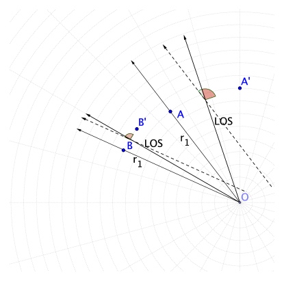
where $\bm{r}_{\text{{-}}}$ connects the two galaxies and $\bm{r}_{\text{{+}}}$ is the vector from the observer to to their midpoint, which we will identify with the LOS of the galaxy pair. Because of local transverse isotropy around the line-of-sight, and our assumption of no WA effects, the CF will only be a function of the distance between the galaxies and the angle they make with respect to the LOS. $\xi(\bm{r}_{1},\bm{r}_{2})=\xi(r_{\text{{-}}},\widehat{\bm{r}}_{\text{{-}}}\widehat{\bm{r}}_{\text{{+}}})$.

The angular dependence of the CF is usually expanded into Legendre polynomials

$$\xi(r_{\text{{-}}},\widehat{\bm{r}}_{\text{{-}}}\widehat{\bm{r}}_{\text{{+}}})=\displaystyle\sum_{\ell}\xi_{\ell}(r_{\text{{-}}})\mathcal{L}_{\ell}(\widehat{\bm{r}}_{\text{{-}}}\widehat{\bm{r}}_{\text{{+}}}),$$ (5)

with most of the useful information in first three even multipoles (Taruya, Saito, & Nishimichi, 2011; Kazin, Sánchez, & Blanton, 2012).

The APS is defined as a FT of CF and can also be decomposed into Legendre polynomials with respect to LOS

$$P(\bm{k})\equiv\displaystyle\int\!\mathrm{d}^{3}r_{\text{{-}}}\,\xi(r_{\text{{-}}},\widehat{\bm{r}}_{\text{{-}}}\widehat{\bm{r}}_{\text{{+}}})\mathrm{e}^{-\mathrm{i}\bm{k}\bm{r}_{\text{{-}}}}=\displaystyle\sum_{\ell}P_{\ell}(k)\mathcal{L}_{\ell}(\widehat{\bm{k}}\widehat{\bm{r}}_{\text{{+}}}).$$ (6)

This is a standard definition and theoretical predictions of APS are computed for this quantity (see e.g., Reimberg, Bernardeau, & Pitrou, 2015, and references therein). The PS multipoles are related to the CF multipoles by

$$P_{\ell}(k)=4\pi\mathrm{i}^{\ell}\displaystyle\int\!\mathrm{d}r_{\text{{-}}}\,\xi_{\ell}(r_{\text{{-}}})j_{\ell}(kr_{\text{{-}}})r_{\text{{-}}}^{2}.$$ (7)

2.1 Pairwise-LOS Method

In the pairwise-LOS method one would correct for the varying LOS, by computing the integral over the overdensity field simultaneously assigning correct LOS direction to all galaxy pairs. In other words, one would compute the multi-dimensional integral

$$P_{\ell}(k)=\frac{2\ell+1}{4\pi V} \displaystyle\int\!\mathrm{d}\widehat{\bm{k}}\mathrm{d}^{3}r_{1}\mathrm{d}^{3}r_{2}$$

$$\delta(\bm{r}_{1})\delta(\bm{r}_{2})\mathrm{e}^{-\mathrm{i}\bm{k}\bm{r}_{1}}\mathrm{e}^{\mathrm{i}\bm{k}\bm{r}_{2}}\mathcal{L}_{\ell}(\widehat{\bm{k}}\widehat{\bm{r}_{\text{{+}}}}).$$ (8)

The expectation value of this integral is

$$P_{\ell}(k)=\frac{2\ell+1}{4\pi V}\displaystyle\int\!\mathrm{d}\widehat{\bm{k}} \mathrm{d}^{3}r_{\text{{-}}}\mathrm{d}^{3}r_{\text{{+}}}$$

$$\xi(r_{\text{{-}}},\widehat{\bm{r}}_{\text{{-}}}\widehat{\bm{r}}_{\text{{+}}})\mathrm{e}^{-\mathrm{i}\bm{k}\bm{r}_{\text{{-}}}}\mathcal{L}_{\ell}(\widehat{\bm{k}}\widehat{\bm{r}_{\text{{+}}}})$$ (9)

and the APS computed in such way would coincide with the definitions of Eq. (6) and (7) and would therefore be exact. Computing this multi-dimensional integral over large galaxy sample however demands prohibitively large CPU time and is not currently viable.

2.2 Single-LOS Method

In the single-LOS method the $\widehat{\bm{z}}$-axis is pointed towards the middle of the survey footprint and it’s assumed that $\widehat{\bm{r}}_{\text{{+}}}\sim\widehat{\bm{z}}$ within the survey volume. This approximation allows us to rewrite Eq. (8) as

$$P_{\ell}(k)=\frac{2\ell+1}{4\pi V}\displaystyle\int\!\mathrm{d}\widehat{\bm{k}}\mathcal{L}_{\ell}(\widehat{\bm{k}}\widehat{\bm{z}})\left|\displaystyle\int\!\mathrm{d}^{3}\bm{r}\delta(\bm{r})\mathrm{e}^{-\mathrm{i}\bm{k}\bm{r}}\right|^{2}.$$ (10)

The expectation value of the integral is

$$P_{\ell}(k)=\frac{2\ell+1}{2}\frac{1}{4\pi}\displaystyle\int\!\mathrm{d}\widehat{\bm{k}}\,P(\bm{k})\mathcal{L}_{\ell}(\widehat{\bm{k}}\widehat{\bm{z}}),$$ (11)

where

$$P(\bm{k})=\frac{1}{V}\displaystyle\iint\!\mathrm{d}^{3}r_{\text{{-}}}\mathrm{d}^{3}r_{\text{{+}}}\xi(r_{\text{{-}}},\widehat{\bm{r}}_{\text{{-}}}\widehat{\bm{r}}_{\text{{+}}})\mathrm{e}^{-\mathrm{i}\bm{k}\bm{r}_{\text{{-}}}},$$ (12)

as before. After integrating over $\bm{r}_{\text{{-}}}$ and $\widehat{\bm{k}}$ this expression reduces to

$$P_{\ell}(k)=P_{\ell}^{\mathrm{t}}(k)\frac{1}{V}\displaystyle\int\!\mathrm{d}^{3}r_{\text{{+}}}\mathcal{L}_{\ell}(\widehat{\bm{z}}\widehat{\bm{r}}_{\text{{+}}}),$$ (13)

where $P^{\mathrm{t}}$ is the true PS multipole defined by Eqs. (6) and (7).

For $\ell=0$ the single-LOS APS reduces to the true APS as $\mathcal{L}_{0}(x)=1$ – The monopole of the APS is unbiased even when measured with the single-LOS method. For higher order multipoles the bias is always present, but could be small in some limits. For example, if the survey area is small and the $\widehat{\bm{z}}$-axis is pointed towards the center of the survey, LOS directions of all pairs will be very close to $\widehat{\bm{z}}$. In this case, $\widehat{\bm{r}}_{\text{{+}}}\sim\widehat{\bm{z}}$ and $\mathcal{L}_{\ell}(\widehat{\bm{z}}\widehat{\bm{r}}_{\text{{+}}})\sim 1$, resulting in small bias.

2.3 Moving-LOS Method

The moving-LOS method is an approximation of Eq. (2.1). The overdensity field is transformed as

$$\tilde{\delta}_{\ell}(\bm{k})=\displaystyle\int\!\mathrm{d}^{3}r\,\delta(\bm{r})\mathcal{L}_{\ell}(\widehat{\bm{k}}\widehat{\bm{r}})\mathrm{e}^{-\mathrm{i}\bm{k}\bm{r}}$$ (14)

and the APS multipoles are computed as

$$P_{\ell}(k)=\frac{2\ell+1}{4\pi V}\displaystyle\int\!\mathrm{d}\widehat{\bm{k}}\tilde{\delta}_{0}(\bm{k})\tilde{\delta}_{\ell}(\bm{k}).$$ (15)

The APS computed in using this expression is equivalent to

$$P_{\ell}(k)=\frac{2\ell+1}{4\pi V} \displaystyle\int\!\mathrm{d}^{3}r_{1}\mathrm{d}^{3}r_{2}\mathrm{d}\widehat{\bm{k}}$$

$$\delta(\bm{r}_{1})\delta(\bm{r}_{2})\mathrm{e}^{-\mathrm{i}\bm{k}\bm{r}_{1}}\mathrm{e}^{\mathrm{i}\bm{k}\bm{r}_{2}}\mathcal{L}_{\ell}(\widehat{\bm{k}}\widehat{\bm{r}_{1}})$$ (16)

and the expectation value of that expression is

$$P_{\ell}(k)=\frac{2\ell+1}{4\pi V}\displaystyle\int\!\mathrm{d}^{3}{r}_{\text{{-}}} \mathrm{d}^{3}r_{\text{{+}}}\mathrm{d}\widehat{\bm{k}}$$

$$\xi(r_{\text{{-}}},\widehat{\bm{r}}_{\text{{-}}}\widehat{\bm{r}}_{\text{{+}}})\mathrm{e}^{-\mathrm{i}\bm{k}\bm{r}_{\text{{-}}}}\mathcal{L}_{\ell}(\widehat{\bm{k}}\widehat{\bm{r}_{1}}).$$ (17)

Using properties of spherical harmonics this can be further reduced to

$$P_{\ell}(k)=\displaystyle\int\!\mathrm{d}k^{\prime}\displaystyle\sum_{\ell^{\prime}}P^{\mathrm{t}}_{\ell^{\prime}}(k^{\prime})W_{\ell\ell^{\prime}}(k,k^{\prime}),$$ (18)

where

$$W_{\ell,\ell^{\prime}}(k,k^{\prime})=\frac{2k^{\prime 2}}{\pi}\displaystyle\int\!\mathrm{d}r_{\text{{-}}}r_{\text{{-}}}^{2}j_{\ell}(kr_{\text{{-}}})j_{\ell^{\prime}}(k^{\prime}r_{\text{{-}}})\mathcal{F}_{\ell\ell^{\prime}}(r_{\text{{-}}})$$ (19)

and

$$\mathcal{F}_{\ell,\ell^{\prime}}(r_{\text{{-}}})\equiv \frac{4\pi\mathrm{i}^{\ell-\ell^{\prime}}}{V(2\ell^{\prime}+1)}\displaystyle\int\!\mathrm{d}^{3}r_{\text{{+}}}\mathrm{d}\widehat{\bm{r}}_{\text{{-}}}$$ (20)

$$\displaystyle\sum_{mm^{\prime}} Y_{\ell^{\prime}m^{\prime}}(\widehat{\bm{r}}_{\text{{-}}})Y^{*}_{\ell^{\prime}m^{\prime}}(\widehat{\bm{r}}_{\text{{+}}})Y^{*}_{\ell m}(\widehat{\bm{r}}_{\text{{-}}})Y_{\ell m}(\widehat{\bm{r}}_{1})$$

(See App. A for details).

This expression will reduce to the true APS only if $W_{\ell\ell^{\prime}}(k,k^{\prime})=\delta_{\ell\ell^{\prime}}\delta(k-k^{\prime})$. In the limit of very small separations $\widehat{\bm{r}}_{\text{{+}}}\sim\widehat{\bm{r}}_{1}$, the $\mathcal{F}$ tends to $\delta_{\ell\ell^{\prime}}$ by the virtue of the closure relation for the spherical harmonics, making $W_{\ell\ell^{\prime}}(k,k^{\prime})$ converge to $\delta_{\ell\ell^{\prime}}\delta(k-k^{\prime})$ in the mean. Properties of spherical harmonics also enforce the condition $W_{0\ell^{\prime}}\propto\delta_{0\ell^{\prime}}$ for all $k$ and $k^{\prime}$, which means that, as with the single-LOS method, there is no bias for $\ell=0$. Unlike the single-LOS method, the bias can’t be expressed as a simple scale-independent scaling of the APS.

3 APS bias as a function of sky area, redshift, and scale

In this section we will quantify the biases in the single-LOS and moving-LOS methods, using the pairwise-LOS method as the reference. To compute the biases we need to specify the geometry of the observed volume as the biases will depend on the distribution of pair separations. For simplicity, we will assume that the observed patch of the sky is circularly symmetric, the $\widehat{\bm{z}}$-axis is pointing to the center of the observed area (this choice results in the least bias for the single-LOS method with the assumed LOS along this direction), and the mask and selection functions are uniform. We will also assume that the width of redshift bin is small compared to the distance of the sample from the observer. This simple model clearly lacks the detailed window of an actual survey, but the angular distribution of pair separations will be roughly correct, and the radial thinness is a conservative choice as it forces pair separations of the same physical separation to wider angular separations.

For this geometry, using a single-LOS analysis the bias, given by Eq. (13), reduces to

$$P_{\ell}(k)=P_{\ell}^{\mathrm{t}}(k)\frac{\displaystyle\int_{0}^{\vartheta_{\mathrm{max}}}\!\!\!\!\!\!\!\!\!\!\!\mathrm{d}\vartheta\,\sin(\vartheta)\mathcal{L}_{\ell}[\cos(\vartheta)]}{\displaystyle\int_{0}^{\vartheta_{\mathrm{max}}}\!\!\!\!\!\!\!\!\!\!\!\mathrm{d}\vartheta\,\sin(\vartheta)}.$$ (21)

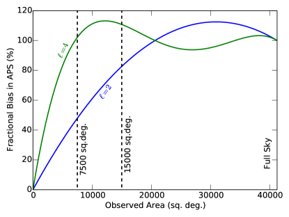
The bias in the APS is independent of the wavenumber and redshift and only depends on the angular extent of the observed area. We plot this bias for $\ell=2$ and $\ell=4$ in Fig. 2. We see a gradual increase in the biases with area for small surveys, with biases that are already larger than 1 per cent when the footprint is only 1000 $\mathrm{deg}^{2}$. For hemispherical or full-sky surveys with a single-LOS, both the quadrupole ($\ell=2$) and the hexadecapole ($\ell=4$) are zero (the fractional error is 1): here any increase in the clustering strength caused by RSD along the single-LOS is matched by an increase perpendicular to the single-LOS around the edges of each hemisphere.

Figure 2: Fractional error in the measured APS as a function of observed area for the single-LOS method.

For the moving-LOS method, the APS bias given by Eq. (18) cannot be expressed as a simple ratio of true and measured power-spectra. For the simple – “thin spherical cap” – geometry we have assumed, we can use the properties of spherical harmonics to reduce the five dimensional integral in Eq. (20) to a one dimensional integral

$$\mathcal{F}_{\ell\ell^{\prime}}(\eta)= \mathrm{i}^{\ell-\ell^{\prime}}\frac{2\ell+1}{2}\displaystyle\int_{-1}^{1}\!\mathrm{d}\mu\,$$ (22)

$$\mathcal{P}_{\ell^{\prime}}^{0}(\mu)\mathcal{P}_{\ell}^{0}(\mu)\mathcal{P}_{\ell}^{0}\left(\frac{1-\eta\mu/2}{\sqrt{1-\eta\mu+\eta^{2}/4}}\right)$$

(see, App. A) where $\mathcal{P}$ denote associated Legendre polynomials and $\eta\equiv r_{\text{{-}}}/r_{\text{{+}}}$. Examining Eq. (22) we see that the expression tends to $\delta_{\ell\ell^{\prime}}$ when $\eta$ tends to zero, suggesting that, for a fixed scale, the approximation works better the further away that galaxies are from the observer, as expected. Eq. (22) also shows that the bias depends only on the wavenumber and doesn’t depend on the observed sky coverage: given that the bias is only related to how each pair of galaxies is treated rather than the distribution of pairs, this is also expected for scales unaffected by the window.

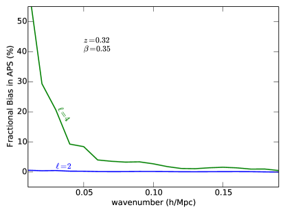
Fig. 3 shows the fractional bias in the APS at $z=0.32$ for $\beta=0.35$. The bias in the quadrupole lies below 1 per cent at wavenumbers above 0.01 $h$/Mpc. The bias in the hexadecapole is larger and reaches a sub per cent level only for wavenumbers above 0.1 $h$/Mpc. At higher redshifts the biases are reduced even further.

Figure 3: Fractional error in the measured APS as a function of observed area for the moving-LOS method for $z=0.32$ and $\beta=0.35$.

4 Summary and Comparison with Previous Work

In this work we quantify biases on the APS measured by various computational methods, focussing on methods correcting for the varying LOS. We have ignored wide-angle effects that arise because the peculiar velocity shifts in galaxies in a pair are not parallel. At 200$h^{\text{{-}}1}$ Mpc this effect is less than a per cent already at $z=0.2$, and decreases for the smaller scales usually of interest in analyses (see e.g. Samushia, Percival, & Raccanelli, 2012; Raccanelli, Samushia, & Percival, 2010). Instead, the approximations discussed in this work are related to the way of measuring the APS, and we have compared two methods - one known to be wrong (single-LOS), and one where small biases have previously been assumed (Blake et al., 2011; Beutler et al., 2014) but that we now quantify (moving-LOS).

To provide a baseline, we have considered ignoring the variation in the LOS and assuming a single-LOS: here we have shown that we are left with a significant bias in measurements other than the monopole moment of the power spectrum, that is independent of scale and only depends on the area of the angular footprint. This has been know for a long time, and consequently this method has not been widely used to measure the APS, other than the monopole. We have shown through an analytic formula for the induced bias of APS multipoles (Eq. 13), that the bias on the quadrupole is large even for surveys as small as 1000 deg². Our results can be used to correct this effect to leading order for analysis methods in which the observed area is subdivided into smaller regions to make the bias smaller (see e.g., Cole, Fisher, & Weinberg, 1994; Hemantha, Wang, & Chuang, 2014).

We have also considered a measurement method proposed more recently, that performs the transform summing over galaxies in a way that allows varying LOS to be factored into the measurement. Ideally we would want to sum over pairs rather than galaxies, but this is impractical, and this revision leads to a small bias in the anisotropic measurements. We have derived an analytic formula for this bais that, in the limit of narrow redshift bin, can be reduced to a one dimensional integral over the true power-spectrum (Eq. 18). This shows that the bias is a function of scale (but not the area) and only depends on the ratio of pair-separation to the distance of pair from the observer $r_{\text{{-}}}/r_{\text{{+}}}$. While small, this correction can easily be calculated and measurements corrected for this effect.

The new method calculating the APS using a sum over galaxies (moving-LOS) remains accurate for the quadrupole APS at scales above $k=0.01h^{-1}$ Mpc even at small redshifts. The bias in the hexadecapole moment is larger, but also decays at high redshifts. Our correction formulas in Eq. (13) and (18) can be used to correct the biases to leading order.

Our analysis of the significance of making various LOS approximations makes a number of simplifying assumptions about the survey for the sake of analytical clarity. We assume the thin-shell approximation and ignore boundary effects, the effects of mask, and the redshift dependence of the mean galaxy number density. While the primary effects of these assumptions can be corrected when making clustering measurements, it is likely that they couple with the geometric biases considered here. Indeed, these approximations are likely to change the corrections due to LOS-assumptions at a comparable order to the corrections presented here for a simplified survey (although when the single-LOS method is used on a data with wide footprint the geometric effects are likely to be dominant). A more precise correction would require a detailed study of how the mask effects couple with the geometric biases.

Appendix A Bias in Moving-LOS Method

We will rewrite Eq. (2.3) using the plane wave expansion,

$$\mathrm{e}^{\mathrm{i}\bm{k}\bm{r}}=\displaystyle\sum_{\ell m}i^{\ell}4\pi j_{\ell}(kr)Y_{\ell m}(\widehat{\bm{k}})Y^{*}_{\ell m}(\widehat{\bm{r}}),$$ (23)

and the addition theorem for Legendre polynomials,

$$\mathcal{L}(\widehat{\bm{k}}\widehat{\bm{r}})=\frac{4\pi}{2\ell+1}\displaystyle\sum_{m}Y_{\ell m}(\widehat{\bm{k}})Y^{*}_{\ell m}(\widehat{\bm{r}}).$$ (24)

This results in

$$P_{\ell}(k)= \frac{2\ell+1}{4\pi V}\displaystyle\sum_{\ell^{\prime}m^{\prime}}\displaystyle\sum_{\ell^{\prime\prime}m^{\prime\prime}}\displaystyle\sum_{m}\displaystyle\int\!\mathrm{d}^{3}r_{\text{{-}}}\mathrm{d}^{3}r_{\text{{+}}}\mathrm{d}\widehat{\bm{k}}$$

$$\xi_{\ell^{\prime}}(r_{\text{{-}}})\frac{4\pi}{2\ell^{\prime}+1}Y_{\ell^{\prime}m^{\prime}}(\widehat{\bm{r}}_{\text{{-}}})Y^{*}_{\ell^{\prime}m^{\prime}}(\widehat{\bm{r}}_{\text{{+}}})$$

$$\mathrm{i}^{\ell^{\prime\prime}}4\pi j_{\ell^{\prime\prime}}(kr)Y^{*}_{\ell^{\prime\prime}m^{\prime\prime}}(\widehat{\bm{k}})Y_{\ell^{\prime\prime}m^{\prime\prime}}(\widehat{\bm{r}}_{\text{{-}}})$$ (25)

$$\frac{4\pi}{2\ell+1}Y_{\ell m}(\widehat{\bm{k}})Y^{*}_{\ell m}(\widehat{\bm{r}}_{1}).$$

Integrating over $\widehat{\bm{k}}$, by virtue of orthogonality of spherical harmonics, results in Eqs. (18)–(20).

The expression in Eq. (20) is invariant under the rotation of coordinate system. This symmetry can be used to align the direction of $\widehat{\bm{z}}$ axis with $\widehat{\bm{r}}_{\text{{+}}}$ as we integrate over $\mathrm{d}\widehat{\bm{r}}_{\text{{+}}}$. Ignoring the boundary effects and assuming that the redshift shell is thin, this results in in

$$\mathcal{F}_{\ell\ell^{\prime}}(r_{\text{{-}}}) =\mathrm{i}^{\ell-\ell^{\prime}}\sqrt{\frac{4\pi}{(2\ell^{\prime}+1)}}$$ (26)

$$\displaystyle\int\!\mathrm{d}\widehat{\bm{r}}_{\text{{-}}}Y_{\ell^{\prime}0}(\widehat{\bm{r}}_{\text{{-}}})\displaystyle\sum_{m}Y^{*}_{\ell m}(\widehat{\bm{r}}_{\text{{-}}})Y_{\ell m}(\widehat{\bm{r}}_{1}),$$

as the integral over $\mathrm{d}^{3}r_{\text{{+}}}$ is equal to volume and only terms with $m^{\prime}=0$ because $\bm{r}_{\text{{+}}}$ is pointing in $\widehat{\bm{z}}$ direction. This expression is again invariant with respect to rotations in azimuthal angle (ignoring boundary effects) and can be reduced to

$$\mathcal{F}_{\ell\ell^{\prime}}(r_{\text{{-}}}) =2\pi\mathrm{i}^{\ell-\ell^{\prime}}\sqrt{\frac{4\pi}{(2\ell^{\prime}+1)}}$$ (27)

$$\displaystyle\int\!\mathrm{d}\mu_{\text{{-}}}Y_{\ell^{\prime}0}(\mu_{\text{{-}}})Y^{*}_{\ell 0}(\mu_{\text{{-}}})Y_{\ell 0}(\mu_{1}),$$

where the $m^{\prime}\neq 0$ terms are killed by the azimuthal integral and $\mu_{\text{{-}}}$ and $\mu_{1}$ are the cosines of respective polar angles. Since $\bm{r}_{1}=\bm{r}_{\text{{+}}}-\bm{r}_{\text{{-}}}/2$ we have $\mu_{1}=(1-\eta\mu_{\text{{-}}}/2)/\sqrt{1-\eta\mu+\eta^{2}/4}$, which will result in Eq. (22).

References

- Alcock & Paczynski (1979) Alcock C., Paczynski B., 1979, Natur, 281, 358
- Anderson et al. (2014) Anderson L., et al., 2014, MNRAS, 441, 24
- Beutler et al. (2012) Beutler F., et al., 2012, MNRAS, 423, 3430
- Beutler et al. (2014) Beutler F., et al., 2014, MNRAS, 443, 1065
- Bianchi et al. (2015) Bianchi D., Gil-Marín H., Ruggeri R., Percival W. J., 2015, arXiv, arXiv:1505.05341
- Blake et al. (2011) Blake C., et al., 2011, MNRAS, 415, 2876
- Cole, Fisher, & Weinberg (1994) Cole S., Fisher K. B., Weinberg D. H., 1994, MNRAS, 267, 785
- Hamilton (1998) Hamilton A. J. S., 1998, ASSL, 231, 185
- Hemantha, Wang, & Chuang (2014) Hemantha M. D. P., Wang Y., Chuang C.-H., 2014, MNRAS, 445, 3737
- Kaiser (1987) Kaiser N., 1987, MNRAS, 227, 1
- Kazin, Sánchez, & Blanton (2012) Kazin E. A., Sánchez A. G., Blanton M. R., 2012, MNRAS, 419, 3223
- Leistedt et al. (2012) Leistedt B., Rassat A., Réfrégier A., Starck J.-L., 2012, A&A, 540, AA60
- Percival et al. (2004) Percival W. J., et al., 2004, MNRAS, 353, 1201
- Raccanelli, Samushia, & Percival (2010) Raccanelli A., Samushia L., Percival W. J., 2010, MNRAS, 409, 1525
- Reimberg, Bernardeau, & Pitrou (2015) Reimberg P. H. F., Bernardeau F., Pitrou C., 2015, arXiv, arXiv:1506.06596
- Samushia, Percival, & Raccanelli (2012) Samushia L., Percival W. J., Raccanelli A., 2012, MNRAS, 420, 2102
- Samushia et al. (2014) Samushia L., et al., 2014, MNRAS, 439, 3504
- Scoccimarro (2015) Scoccimarro R., 2015, arXiv, arXiv:1506.02729
- Szalay, Matsubara, & Landy (1998) Szalay A. S., Matsubara T., Landy S. D., 1998, ApJ, 498, L1
- Szapudi (2004) Szapudi I., 2004, ApJ, 614, 51
- Tadros et al. (1999) Tadros H., et al., 1999, MNRAS, 305, 527
- Taruya, Saito, & Nishimichi (2011) Taruya A., Saito S., Nishimichi T., 2011, PhRvD, 83, 103527
- Yamamoto et al. (2006) Yamamoto K., Nakamichi M., Kamino A., Bassett B. A., Nishioka H., 2006, PASJ, 58, 93
- Yoo & Seljak (2015) Yoo J., Seljak U., 2015, MNRAS, 447, 1789