How clustering dark energy affects matter perturbations

A. Mehrabi1, S. Basilakos2 and F. Pace3
1 Department of Physics, Bu-Ali Sina University, Hamedan 65178, Iran
2 Academy of Athens, Research Center for Astronomy & Applied Mathematics, Soranou Efessiou 4, 11-527, Athens, Greece
3 Jodrell Bank Centre for Astrophysics, School of Physics and Astronomy, The University of Manchester, Manchester, M13ย 9PL, UK
mehrabi@basu.ac.irsvasil@academyofathens.gr
(Accepted ?, Received ?; in original form )
Abstract

The rate of structure formation in the Universe is different in homogeneous and clustered dark energy models. The degree of dark energy clustering depends on the magnitude of its effective sound speed ceff2subscriptsuperscript๐‘2effc^{2}_{\rm eff} and for ceff=0subscript๐‘eff0c_{\rm eff}=0 dark energy clusters in a similar fashion to dark matter while for ceff=1subscript๐‘eff1c_{\rm eff}=1 it stays (approximately) homogeneous. In this paper we consider two distinct equations of state for the dark energy component, wd=cโ€‹oโ€‹nโ€‹sโ€‹tsubscript๐‘คd๐‘๐‘œ๐‘›๐‘ ๐‘กw_{\rm d}=const and wd=w0+w1โ€‹(z1+z)subscript๐‘คdsubscript๐‘ค0subscript๐‘ค1๐‘ง1๐‘งw_{\rm d}=w_{0}+w_{1}\left(\frac{z}{1+z}\right) with ceffsubscript๐‘effc_{\rm eff} as a free parameter and we try to constrain the dark energy effective sound speed using current available data including SnIa, Baryon Acoustic Oscillation, CMB shift parameter (Planck and WMAP), Hubble parameter, Big Bang Nucleosynthesis and the growth rate of structures fโ€‹ฯƒ8โ€‹(z)๐‘“subscript๐œŽ8๐‘งf\sigma_{8}(z). At first we derive the most general form of the equations governing dark matter and dark energy clustering under the assumption that ceff=cโ€‹oโ€‹nโ€‹sโ€‹tsubscript๐‘eff๐‘๐‘œ๐‘›๐‘ ๐‘กc_{\rm eff}=const. Finally, performing an overall likelihood analysis we find that the likelihood function peaks at ceff=0subscript๐‘eff0c_{\rm eff}=0, however the dark energy sound speed is degenerate with respect to the cosmological parameters, namely ฮฉmsubscriptฮฉm\Omega_{\rm m} and wdsubscript๐‘คdw_{\rm d}.

keywords:
Methods: analytic โ€“ cosmological parameters โ€“ cosmology: theory โ€“ dark energy

1 Introduction

We are living in a special epoch of the cosmic history where the expansion of the Universe is accelerated due to an unknown energy component, usually dubbed dark energy (DE). This acceleration has been discovered observationally using the luminosity distance of Type Ia supernovae (SnIa) (Perlmutter etย al., 1997, 1998, 1999; Riess etย al., 2004; Astier etย al., 2006; Jha etย al., 2007). In addition to this, other observations including the cosmic microwave background (CMB) (Bennett etย al., 2003; Spergel etย al., 2003, 2007; Planck Collaboration XIII, 2015; Planck Collaboration XIV, 2015), large scale structures (LSS) (Hawkins etย al., 2003; Tegmark etย al., 2004; Cole etย al., 2005) and baryon acoustic oscillation (BAO) (Eisenstein etย al., 2005; Seo & Eisenstein, 2005; Blake etย al., 2011) support an accelerated expansion. At a fundamental level there are two different approaches to describe the phenomenon of the cosmic acceleration and indeed many efforts are devoted to investigate its deep nature both observationally and theoretically. One way is to consider a fluid with a sufficiently negative pressure dubbed DE and the other is based on the modification of the laws of gravity on large scales. The first approach comes in many different scenarios. The simplest one is a very tiny cosmological constant ฮ›ฮ›\Lambda in Einstein field equations that has a (negative) pressure equal to its energy density and equation-of-state parameter wd=pdฯd=โˆ’1subscript๐‘คdsubscript๐‘dsubscript๐œŒd1w_{\rm d}=\frac{p_{\rm d}}{\rho_{\rm d}}=-1 (Weinberg, 1989; Sahni & Starobinsky, 2000; Peebles & Ratra, 2003). The overall theoretical cosmological model (cosmological constant plus cold dark matter to explain galaxy rotation curves and the potential well for structure formation) is called ฮ›ฮ›\LambdaCDM model. Despite being highly consistent with observational data, the ฮ›ฮ›\LambdaCDM model suffers of two theoretical problems, namely the fine-tuning and the cosmic coincidence problem (Weinberg, 1989; Sahni & Starobinsky, 2000; Peebles & Ratra, 2003). Differently from the cosmological constant case with equation of state (EoS) wd=โˆ’1subscript๐‘คd1w_{\rm d}=-1, other dynamical models have been largely studied in the literature and usually categorised in two branches, quintessence models (Armendariz-Picon etย al., 2000; Copeland etย al., 2006) and k-essence models (Armendariz-Picon etย al., 1999, 2000; Chiba etย al., 2000, 2009; Amendola & Tsujikawa, 2010).

The simplest way to modify gravity is to consider Einstein-Hilbert Lagrangian as a generic function of the Ricci scalar R๐‘…R (fโ€‹(R)๐‘“๐‘…f(R) theories, Schmidt, 1990; Magnano & Sokolowski, 1994; Dobado & Maroto, 1995; Capozziello etย al., 2003; Carroll etย al., 2004) or add extra-dimension models like in the DGP model (Dvali, Gabadadze & Porrati, 2000). Understanding which class of models is the real one is one of the biggest challenges for cosmology.

In addition to the background evolution, large scale structures provide valuable information about the nature of dark energy (Tegmark etย al., 2004, 2006). Primordial matter perturbations grow throughout the cosmic history and their growth rate depends on the overall energy budget and on the properties of the cosmic fluids. DE slows down the growth rate of large-scale structures. Structures grow due to gravitational instability and DE acts opposing and reducing the growth rate. The growth rate of structures can be measured from the redshift space distortion (RSD). Inward peculiar velocities of large-scale structures generate a distortion that is directly related to the matter density contrast.

Since the cosmological constant does not change in space and time, it can not cluster like dark matter (DM) and it has a negligible contribution to the energy density of the universe at high redshift. On the other hand, dynamical DE can cluster and the amount of clustering depends strongly on its effective sound speed. The effective sound speed is defined as ceff2=ce=ฮดโ€‹pdฮดโ€‹ฯdsuperscriptsubscript๐‘eff2subscript๐‘e๐›ฟsubscript๐‘d๐›ฟsubscript๐œŒdc_{\rm eff}^{2}=c_{\rm e}=\frac{\delta p_{\rm d}}{\delta\rho_{\rm d}} (hereafter we use cesubscript๐‘ec_{\rm e}) where ฮดโ€‹pd๐›ฟsubscript๐‘d\delta p_{\rm d} and ฮดโ€‹ฯd๐›ฟsubscript๐œŒd\delta\rho_{\rm d} are the pressure and energy density perturbations for DE respectively and coincides with the actual sound speed in the dark energy comoving rest frame (Hu, 1998). In quintessence models we have ceโ‰ƒ1similar-to-or-equalssubscript๐‘e1c_{\rm e}\simeq 1 so DE perturbations can not grow on sub-horizon scales while in k-essence models the effective sound speed can be tiny (ceโ‰ช1much-less-thansubscript๐‘e1c_{\rm e}\ll 1) (Garriga & Mukhanov, 1999; Armendariz-Picon etย al., 1999, 2000; Babichev etย al., 2006; Akhoury etย al., 2011) and DE perturbations grow similarly to dark matter (DM) perturbations. The possibility of DE clustering has been studied by many authors (Erickson etย al., 2002; Bean & Dorรฉ, 2004; Hu & Scranton, 2004; Ballesteros & Riotto, 2008; deย Putter etย al., 2010; Sapone & Majerotto, 2012; Batista & Pace, 2013; Dossett & Ishak, 2013; Basse etย al., 2014; Batista, 2014; Pace etย al., 2014; Steigerwald etย al., 2014). In particular, it has been shown that the homogeneous DE scenario fails to reproduce the observed concentration parameter of the massive galaxy clusters (Basilakos etย al., 2009). In this framework, deย Putter etย al. (2010) pointed out that CMB and LSS slightly prefer dynamical DE with ceโ‰ 1subscript๐‘e1c_{\rm e}\neq 1 and recently Mehrabi, Malekjani & Pace (2015) and Basilakos (2015) have shown that clustering DE reproduces the growth data better in the framework of the spherical collapse model. A similar conclusion was suggested also by Nesseris & Sapone (2014).

The growth rate f=dโ€‹lnโกฮดmdโ€‹lnโกa๐‘“๐‘‘subscript๐›ฟm๐‘‘๐‘Žf=\frac{d\ln\delta_{\rm m}}{d\ln a} is usually approximated by f=ฮฉmฮณ๐‘“superscriptsubscriptฮฉm๐›พf=\Omega_{\rm m}^{\gamma} as first introduced by Peebles (1993). In this parametrization ฮณ๐›พ\gamma is the so called growth index and can be used to distinguish between DE and modified gravity models (Linder, 2005; Huterer & Linder, 2007; Basilakos & Pouri, 2012; Rapetti etย al., 2013). It is well known that for a ฮ›ฮ›\LambdaCDM model ฮณ๐›พ\gamma is independent of redshift and equal to 6/116116/11. The evolution of the matter density ฮฉmsubscriptฮฉm\Omega_{\rm m} depends on the evolution of the Hubble parameter Hโ€‹(a)๐ป๐‘ŽH(a) and hence on the particular cosmological model adopted. In this paper we consider two distinct models, a constant wdsubscript๐‘คdw_{\rm d} and a dynamical wdโ€‹(z)subscript๐‘คd๐‘งw_{\rm d}(z), and we consider ceffsubscript๐‘effc_{\rm eff} as a free parameter. Then based on the linear regime we numerically solve the perturbed general relativity (GR) equations to evaluate the growth rate of matter in the presence of DE clustering. Using a Markov Chain Monte Carlo (MCMC) method we can constrain the cosmological parameters using SnIa, BAO, CMB shift parameter, the Hubble parameter, the Big Bang Nucleosynthesis (BBN) and growth rate data fโ€‹ฯƒ8โ€‹(z)๐‘“subscript๐œŽ8๐‘งf\sigma_{8}(z).

The structure of this paper is as follows. In sectionย 2 we derive the equations governing the linear growth of matter perturbations in a general relativistic framework and show the effects of DE clustering on the growth rate of matter. In sectionย 3 we present all the details of the observational data used in this work to constrain the cosmological parameters including the DE sound speed and their uncertainties. In sectionย 4, we provide for the first time (to our knowledge) an approximated solution of the growth index of matter fluctuations as a function of the cosmological parameters, DE perturbations and cesubscript๐‘ec_{\rm e}. Finally in sectionย 5 we conclude and discuss our results.

2 Effect of dark energy sound speed on the growth rate of matter perturbations

In this section we revise the fundamental equations necessary to our analysis. The sound horizon of DE with effective sound speed cesubscript๐‘ec_{\rm e} in a FRW universe is given by:

ฮปsโ€‹(a)=โˆซaiaceโ€‹(x)xโ€‹โ„‹โ€‹(x)โ€‹๐‘‘x,subscript๐œ†s๐‘Žsuperscriptsubscriptsubscript๐‘Ži๐‘Žsubscript๐‘e๐‘ฅ๐‘ฅโ„‹๐‘ฅdifferential-d๐‘ฅ\lambda_{\rm s}(a)=\int_{a_{\rm i}}^{a}\frac{c_{\rm e}(x)}{x\mathcal{H}(x)}\leavevmode\nobreak\ dx\;, (1)

where โ„‹=aโ€ฒaโ„‹superscript๐‘Žโ€ฒ๐‘Ž\mathcal{H}=\frac{a^{\prime}}{a}, the prime being the derivative with respect to conformal time (ฮท๐œ‚\eta) and aisubscript๐‘Žia_{\rm i} an initial scale factor. The nominal Hubble parameter is given by H=aห™a๐ปห™๐‘Ž๐‘ŽH=\frac{\dot{a}}{a} and thus โ„‹=aโ€‹Hโ„‹๐‘Ž๐ป\mathcal{H}=aH which implies

โ„‹โ€ฒโ„‹2=1+Hห™H2,superscriptโ„‹โ€ฒsuperscriptโ„‹21ห™๐ปsuperscript๐ป2\frac{\mathcal{H}^{\prime}}{\mathcal{H}^{2}}=1+\frac{\dot{H}}{H^{2}}\;, (2)

where an overdot refers to a derivative with respect to the cosmic time (t๐‘กt). In the case of ceโ‰ƒ1similar-to-or-equalssubscript๐‘e1c_{\rm e}\simeq 1, pressure suppresses any DE perturbation with the consequence that DE may cluster only on scales comparable to the horizon.

The opposite situation holds if ceโ‰ช1much-less-thansubscript๐‘e1c_{\rm e}\ll 1. Indeed in this case DE can cluster in analogy to the DM component and perturbations will grow with time. DE clustering modifies the evolution of DM perturbation and thus it affects the rate of structure formation in the universe.

We start our derivation of the relevant equations by considering the line element of an expanding universe in the Newtonian gauge without anisotropic stress:

dโ€‹s2=โˆ’(1+2โ€‹ฯ•)โ€‹dโ€‹t2+a2โ€‹(t)โ€‹(1โˆ’2โ€‹ฯ•)โ€‹dโ€‹xโ†’2,๐‘‘superscript๐‘ 212italic-ฯ•๐‘‘superscript๐‘ก2superscript๐‘Ž2๐‘ก12italic-ฯ•๐‘‘superscriptโ†’๐‘ฅ2ds^{2}=-(1+2\phi)dt^{2}+a^{2}(t)(1-2\phi)d\vec{x}^{2}\;, (3)

where ฯ•italic-ฯ•\phi is the Bardeen potential. First-order Einstein equations in Fourier space are:

3โ€‹โ„‹โ€‹ฯ•โ€ฒ+(3โ€‹โ„‹2+k2)โ€‹ฯ•3โ„‹superscriptitalic-ฯ•โ€ฒ3superscriptโ„‹2superscript๐‘˜2italic-ฯ•\displaystyle 3\mathcal{H}\phi^{\prime}+\left(3\mathcal{H}^{2}+k^{2}\right)\phi =\displaystyle= โˆ’3โ€‹โ„‹22โ€‹(ฮฉmโ€‹ฮดm+ฮฉdโ€‹ฮดd),3superscriptโ„‹22subscriptฮฉmsubscript๐›ฟmsubscriptฮฉdsubscript๐›ฟd\displaystyle-\frac{3\mathcal{H}^{2}}{2}(\Omega_{\rm m}\delta_{\rm m}+\Omega_{\rm d}\delta_{\rm d})\;, (4)
ฯ•โ€ฒโ€ฒ+3โ€‹โ„‹โ€‹ฯ•โ€ฒ+(2โ€‹aโ€ฒโ€ฒaโˆ’โ„‹2)โ€‹ฯ•superscriptitalic-ฯ•โ€ฒโ€ฒ3โ„‹superscriptitalic-ฯ•โ€ฒ2superscript๐‘Žโ€ฒโ€ฒ๐‘Žsuperscriptโ„‹2italic-ฯ•\displaystyle\phi^{\prime\prime}+3\mathcal{H}\phi^{\prime}+\left(\frac{2a^{\prime\prime}}{a}-\mathcal{H}^{2}\right)\phi =\displaystyle= 3โ€‹โ„‹22โ€‹ฮฉdโ€‹ฮดโ€‹pdฮดโ€‹ฯdโ€‹ฮดd,3superscriptโ„‹22subscriptฮฉd๐›ฟsubscript๐‘d๐›ฟsubscript๐œŒdsubscript๐›ฟd\displaystyle\frac{3\mathcal{H}^{2}}{2}\Omega_{\rm d}\frac{\delta p_{\rm d}}{\delta\rho_{\rm d}}\delta_{\rm d}\;, (5)

where ฮฉm=ฮฉDM+ฮฉbsubscriptฮฉmsubscriptฮฉDMsubscriptฮฉb\Omega_{\rm m}=\Omega_{\rm DM}+\Omega_{\rm b} (ฮฉd=1โˆ’ฮฉmsubscriptฮฉd1subscriptฮฉm\Omega_{\rm d}=1-\Omega_{\rm m}) is the matter (dark energy) density parameter and ฮดmsubscript๐›ฟm\delta_{\rm m} (ฮดdsubscript๐›ฟd\delta_{\rm d}) is the corresponding density contrast. The first-order energy-momentum conservation equations for a generic fluid with equation-of-state parameter w๐‘คw are (Ma & Bertschinger, 1995)

ฮดโ€ฒsuperscript๐›ฟโ€ฒ\displaystyle\delta^{\prime} =\displaystyle= โˆ’(1+w)โ€‹(ฮธโˆ’3โ€‹ฯ•โ€ฒ)โˆ’3โ€‹aโ€ฒaโ€‹(ฮดโ€‹pฮดโ€‹ฯโˆ’w)โ€‹ฮด,1๐‘ค๐œƒ3superscriptitalic-ฯ•โ€ฒ3superscript๐‘Žโ€ฒ๐‘Ž๐›ฟ๐‘๐›ฟ๐œŒ๐‘ค๐›ฟ\displaystyle-(1+w)(\theta-3\phi^{\prime})-3\frac{a^{\prime}}{a}\left(\frac{\delta p}{\delta\rho}-w\right)\delta\;, (6)
ฮธโ€ฒsuperscript๐œƒโ€ฒ\displaystyle\theta^{\prime} =\displaystyle= โˆ’aโ€ฒaโ€‹(1โˆ’3โ€‹w)โ€‹ฮธโˆ’wโ€ฒ1+wโ€‹ฮธ+ฮดโ€‹pฮดโ€‹ฯ1+wโ€‹k2โ€‹ฮด+k2โ€‹ฯ•.superscript๐‘Žโ€ฒ๐‘Ž13๐‘ค๐œƒsuperscript๐‘คโ€ฒ1๐‘ค๐œƒ๐›ฟ๐‘๐›ฟ๐œŒ1๐‘คsuperscript๐‘˜2๐›ฟsuperscript๐‘˜2italic-ฯ•\displaystyle-\frac{a^{\prime}}{a}(1-3w)\theta-\frac{w^{\prime}}{1+w}\theta+\frac{\frac{\delta p}{\delta\rho}}{1+w}k^{2}\delta+k^{2}\phi\;. (7)

These equations are correct for any fluid with p=wโ€‹ฯ๐‘๐‘ค๐œŒp=w\rho (for dust w=0๐‘ค0w=0 and for dark energy w=wd๐‘คsubscript๐‘คdw=w_{\rm d}), where ฮด๐›ฟ\delta is the density contrast, ฮธ๐œƒ\theta is the divergence of the fluid velocity (ฮธ=iโ€‹kiโ€‹vi๐œƒ๐‘–superscript๐‘˜๐‘–subscript๐‘ฃ๐‘–\theta=ik^{i}v_{i}) and ฮดโ€‹pฮดโ€‹ฯ๐›ฟ๐‘๐›ฟ๐œŒ\frac{\delta p}{\delta\rho} can be written as (Bean & Dorรฉ, 2004)

ฮดโ€‹pฮดโ€‹ฯ=ce+3โ€‹โ„‹โ€‹(1+w)โ€‹(ceโˆ’cad2)โ€‹ฮธฮดโ€‹1k2,๐›ฟ๐‘๐›ฟ๐œŒsubscript๐‘e3โ„‹1๐‘คsubscript๐‘esuperscriptsubscript๐‘ad2๐œƒ๐›ฟ1superscript๐‘˜2\frac{\delta p}{\delta\rho}=c_{\rm e}+3\mathcal{H}(1+w)(c_{\rm e}-c_{\rm ad}^{2})\frac{\theta}{\delta}\frac{1}{k^{2}}\;, (8)

where ca2=casuperscriptsubscript๐‘a2subscript๐‘ac_{\rm a}^{2}=c_{\rm a} is the DE adiabatic sound speed:

ca=wโˆ’wโ€ฒ3โ€‹โ„‹โ€‹(1+w).subscript๐‘a๐‘คsuperscript๐‘คโ€ฒ3โ„‹1๐‘คc_{\rm a}=w-\frac{w^{\prime}}{3\mathcal{H}(1+w)}\;. (9)

Note that the second term in the right hand side of Eq.ย (8) appears because we demand pressure perturbations to be a gauge invariant quantity (Bean & Dorรฉ, 2004). For a perfect fluid, perturbations in the pressure are purely determined by the adiabatic sound speed but for an imperfect fluid dissipative processes generate entropic perturbations and therefore we have a more general relation. In this case, cesubscript๐‘ec_{\rm e} acts like a proxy for pressure perturbations and the growth of perturbation in the DE component depends on the effective sound speed and not on the adiabatic sound speed any more. In the following this statement will be confirmed by solving the perturbed equations numerically.

To study the effect of the DE sound speed on structure formation, we consider a universe with pressure-less DM and a DE component with varying equation of state that we specialise to wdโ€‹(z)=w0+w1โ€‹z1+zsubscript๐‘คd๐‘งsubscript๐‘ค0subscript๐‘ค1๐‘ง1๐‘งw_{\rm d}(z)=w_{0}+w_{1}\frac{z}{1+z}. The latter parametrization is the well known Chevallier-Polarski-Linder (CPL) parametrization (Chevallier & Polarski, 2001; Linder, 2003). We eliminate ฮธ๐œƒ\theta from Eqs.ย (6) andย (7) and find two second order differential equations for the density contrast of DM and DE. In addition using ddโ€‹ฮท=aโ€‹โ„‹โ€‹ddโ€‹a๐‘‘๐‘‘๐œ‚๐‘Žโ„‹๐‘‘๐‘‘๐‘Ž\frac{d}{d\eta}=a\mathcal{H}\frac{d}{da} and d2dโ€‹ฮท2=a2โ€‹โ„‹2โ€‹d2dโ€‹a2+(aโ€‹โ„‹2+aโ€‹โ„‹ห™)โ€‹ddโ€‹asuperscript๐‘‘2๐‘‘superscript๐œ‚2superscript๐‘Ž2superscriptโ„‹2superscript๐‘‘2๐‘‘superscript๐‘Ž2๐‘Žsuperscriptโ„‹2๐‘Žห™โ„‹๐‘‘๐‘‘๐‘Ž\frac{d^{2}}{d\eta^{2}}=a^{2}\mathcal{H}^{2}\frac{d^{2}}{da^{2}}+(a\mathcal{H}^{2}+a\dot{\mathcal{H}})\frac{d}{da}, these equations can be written in terms of the scale factor. Finally our desired equations governing the growth of DM and DE perturbations are:

d2โ€‹ฮดmdโ€‹a2+Amโ€‹dโ€‹ฮดmdโ€‹a+Bmโ€‹ฮดmsuperscript๐‘‘2subscript๐›ฟm๐‘‘superscript๐‘Ž2subscript๐ดm๐‘‘subscript๐›ฟm๐‘‘๐‘Žsubscript๐ตmsubscript๐›ฟm\displaystyle\frac{d^{2}\delta_{\rm m}}{da^{2}}+A_{\rm m}\frac{d\delta_{\rm m}}{da}+B_{\rm m}\delta_{\rm m} =\displaystyle= Sm,subscript๐‘†m\displaystyle S_{\rm m}\;, (10)
d2โ€‹ฮดddโ€‹a2+Adโ€‹dโ€‹ฮดddโ€‹a+Bdโ€‹ฮดdsuperscript๐‘‘2subscript๐›ฟd๐‘‘superscript๐‘Ž2subscript๐ดd๐‘‘subscript๐›ฟd๐‘‘๐‘Žsubscript๐ตdsubscript๐›ฟd\displaystyle\frac{d^{2}\delta_{\rm d}}{da^{2}}+A_{\rm d}\frac{d\delta_{\rm d}}{da}+B_{\rm d}\delta_{\rm d} =\displaystyle= Sd,subscript๐‘†d\displaystyle S_{\rm d}\;, (11)

and the coefficients [see also Eq.ย (2)] are:

Amsubscript๐ดm\displaystyle A_{\rm m} =\displaystyle= 1aโ€‹(2+โ„‹โ€ฒโ„‹2)=1aโ€‹(3+Hห™H2),1๐‘Ž2superscriptโ„‹โ€ฒsuperscriptโ„‹21๐‘Ž3ห™๐ปsuperscript๐ป2\displaystyle\frac{1}{a}\left(2+\frac{\mathcal{H}^{\prime}}{\mathcal{H}^{2}}\right)=\frac{1}{a}\left(3+\frac{\dot{H}}{H^{2}}\right)\;, (12)
Bmsubscript๐ตm\displaystyle B_{\rm m} =\displaystyle= 0,0\displaystyle 0\;,
Smsubscript๐‘†m\displaystyle S_{\rm m} =\displaystyle= 3โ€‹d2โ€‹ฯ•dโ€‹a2+3aโ€‹[2+โ„‹โ€ฒโ„‹2]โ€‹dโ€‹ฯ•dโ€‹aโˆ’k2a2โ€‹โ„‹2โ€‹ฯ•,3superscript๐‘‘2italic-ฯ•๐‘‘superscript๐‘Ž23๐‘Ždelimited-[]2superscriptโ„‹โ€ฒsuperscriptโ„‹2๐‘‘italic-ฯ•๐‘‘๐‘Žsuperscript๐‘˜2superscript๐‘Ž2superscriptโ„‹2italic-ฯ•\displaystyle 3\frac{d^{2}\phi}{da^{2}}+\frac{3}{a}\left[2+\frac{\mathcal{H}^{\prime}}{\mathcal{H}^{2}}\right]\frac{d\phi}{da}-\frac{k^{2}}{a^{2}\mathcal{H}^{2}}\phi\;,
Adsubscript๐ดd\displaystyle A_{\rm d} =\displaystyle= 1aโ€‹[2+โ„‹โ€ฒโ„‹2+3โ€‹caโˆ’6โ€‹wd],1๐‘Ždelimited-[]2superscriptโ„‹โ€ฒsuperscriptโ„‹23subscript๐‘a6subscript๐‘คd\displaystyle\frac{1}{a}\left[2+\frac{\mathcal{H}^{\prime}}{\mathcal{H}^{2}}+3c_{\rm a}-6w_{\rm d}\right]\;,
Bdsubscript๐ตd\displaystyle B_{\rm d} =\displaystyle= 1a2[3(ceโˆ’wd)(1+โ„‹โ€ฒโ„‹2โˆ’3wd+3caโˆ’3ce)\displaystyle\frac{1}{a^{2}}\left[3\left(c_{\rm e}-w_{\rm d}\right)\left(1+\frac{\mathcal{H}^{\prime}}{\mathcal{H}^{2}}-3w_{\rm d}+3c_{\rm a}-3c_{\rm e}\right)\right.\;
+\displaystyle+ k2โ„‹2ceโˆ’3adโ€‹wddโ€‹a],\displaystyle\left.\frac{k^{2}}{\mathcal{H}^{2}}c_{\rm e}-3a\frac{dw_{\rm d}}{da}\right]\;,
Sdsubscript๐‘†d\displaystyle S_{\rm d} =\displaystyle= (1+wd)[3d2โ€‹ฯ•dโ€‹a2+3a(2+โ„‹โ€ฒโ„‹2โˆ’3ca)dโ€‹ฯ•dโ€‹a\displaystyle(1+w_{\rm d})\left[3\frac{d^{2}\phi}{da^{2}}+\frac{3}{a}\left(2+\frac{\mathcal{H}^{\prime}}{\mathcal{H}^{2}}-3c_{\rm a}\right)\frac{d\phi}{da}\right.\;
โˆ’\displaystyle- k2a2โ€‹โ„‹2ฯ•+31+wddโ€‹ฯ•dโ€‹adโ€‹wddโ€‹a],\displaystyle\left.\frac{k^{2}}{a^{2}\mathcal{H}^{2}}\phi+\frac{3}{1+w_{\rm d}}\frac{d\phi}{da}\frac{dw_{\rm d}}{da}\right]\;,

where โ„‹โ€ฒโ„‹2superscriptโ„‹โ€ฒsuperscriptโ„‹2\frac{\mathcal{H}^{\prime}}{\mathcal{H}^{2}} (or Hห™H2ห™๐ปsuperscript๐ป2\frac{\dot{H}}{H^{2}}) is a function of the scale factor and using Friedmann equations we have

โ„‹โ€ฒโ„‹2=โˆ’12โ€‹ฮฉm+ฮฉdโ€‹(1+3โ€‹wd)ฮฉm+ฮฉd=โˆ’12โ€‹(1+3โ€‹ฮฉdโ€‹wd),superscriptโ„‹โ€ฒsuperscriptโ„‹212subscriptฮฉmsubscriptฮฉd13subscript๐‘คdsubscriptฮฉmsubscriptฮฉd1213subscriptฮฉdsubscript๐‘คd\frac{\mathcal{H}^{\prime}}{\mathcal{H}^{2}}=-\frac{1}{2}\frac{\Omega_{\rm m}+\Omega_{\rm d}(1+3w_{\rm d})}{\Omega_{\rm m}+\Omega_{\rm d}}=-\frac{1}{2}(1+3\Omega_{\rm d}w_{\rm d})\;, (13)

These equations are not in agreement with Eq. (44) in Abramo etย al. (2009), which were obtained in the limit of a matter dominated universe (โ„‹โ€ฒโ„‹2=โˆ’12superscriptโ„‹โ€ฒsuperscriptโ„‹212\frac{\mathcal{H}^{\prime}}{\mathcal{H}^{2}}=-\frac{1}{2}) and a constant wdsubscript๐‘คdw_{\rm d}. To resolve this discrepancy, see appendixย (A).

We integrate Eqs.ย (10) andย (11) numerically from zi=100subscript๐‘งi100z_{\rm i}=100 to z=0๐‘ง0z=0, in order to obtain the density contrast of DM and DE. We use the same procedure of Abramo etย al. (2009) to find the initial conditions. In the matter dominated era ฯ•โ€ฒโ‰ƒ0similar-to-or-equalssuperscriptitalic-ฯ•โ€ฒ0\phi^{\prime}\simeq 0, so from Eq.ย (4) we have:

ฮดm,i=โˆ’2โ€‹ฯ•iโ€‹(1+k23โ€‹โ„‹i2),subscript๐›ฟmi2subscriptitalic-ฯ•i1superscript๐‘˜23superscriptsubscriptโ„‹i2\delta_{\rm m,i}=-2\phi_{\rm i}\left(1+\frac{k^{2}}{3\mathcal{H_{\rm i}}^{2}}\right)\;, (14)

for the initial value of ฮดmsubscript๐›ฟm\delta_{\rm m} and

dโ€‹ฮดm,idโ€‹a=โˆ’23โ€‹k2โ„‹i2โ€‹ฯ•i,๐‘‘subscript๐›ฟmi๐‘‘๐‘Ž23superscript๐‘˜2superscriptsubscriptโ„‹i2subscriptitalic-ฯ•i\frac{d\delta_{\rm m,i}}{da}=-\frac{2}{3}\frac{k^{2}}{\mathcal{H_{\rm i}}^{2}}\phi_{\rm i}\;, (15)

for its derivative. For ฮดdsubscript๐›ฟd\delta_{\rm d} the initial value is set using the adiabatic perturbations condition (Kodama & Sasaki, 1984; Amendola & Tsujikawa, 2010),

ฮดd,i=(1+wd)โ€‹ฮดm,i,subscript๐›ฟdi1subscript๐‘คdsubscript๐›ฟmi\delta_{\rm d,i}=(1+w_{\rm d})\delta_{\rm m,i}\;, (16)

and its derivative is set to

dโ€‹ฮดd,idโ€‹a=(1+wd)โ€‹dโ€‹ฮดm,idโ€‹a+dโ€‹wddโ€‹aโ€‹ฮดm,i.๐‘‘subscript๐›ฟdi๐‘‘๐‘Ž1subscript๐‘คd๐‘‘subscript๐›ฟmi๐‘‘๐‘Ž๐‘‘subscript๐‘คd๐‘‘๐‘Žsubscript๐›ฟmi\frac{d\delta_{\rm d,i}}{da}=(1+w_{\rm d})\frac{d\delta_{\rm m,i}}{da}+\frac{dw_{\rm d}}{da}\delta_{\rm m,i}\;. (17)

According to the above argument, by fixing the initial condition of ฯ•isubscriptitalic-ฯ•i\phi_{\rm i} we have all the initial conditions. We set ฯ•i=โˆ’6ร—10โˆ’7subscriptitalic-ฯ•i6superscript107\phi_{\rm i}=-6\times 10^{-7} which corresponds to ฮดm=0.1subscript๐›ฟm0.1\delta_{\rm m}=0.1 at present time for k=0.1โ€‹hโ€‹Mโ€‹pโ€‹cโˆ’1๐‘˜0.1โ„Ž๐‘€๐‘superscript๐‘1k=0.1hMpc^{-1}. Our results are robust under small changes of the initial conditions, and we donโ€™t worry about the exact values. (For ฯ•i=โˆ’7ร—10โˆ’8subscriptitalic-ฯ•i7superscript108\phi_{\rm i}=-7\times 10^{-8}, ฮดmsubscript๐›ฟm\delta_{\rm m} reach to 0.010.010.01 at present time but fโ€‹ฯƒ8๐‘“subscript๐œŽ8f\sigma_{8} differs less than 10โˆ’4%percentsuperscript10410^{-4}\%.)

DE clustering affects the growth of matter perturbations through the change of the potential ฯ•italic-ฯ•\phi. As we noticed the amount of DE clustering is directly related to its effective sound speed. We restrict our analysis to the choice of k=1/ฮป=0.1โ€‹h๐‘˜1๐œ†0.1โ„Žk=1/\lambda=0.1hMpc-1 which corresponds to ฮป=10โ€‹hโˆ’1๐œ†10superscriptโ„Ž1\lambda=10h^{-1}Mpc (Zhang etย al., 2012). Note that the power-spectrum normalization ฯƒ8subscript๐œŽ8\sigma_{8} which is the rms mass fluctuation on a scale R8=8โ€‹hโˆ’1subscript๐‘…88superscriptโ„Ž1R_{8}=8h^{-1}Mpc corresponds to k=0.125โ€‹h๐‘˜0.125โ„Žk=0.125hMpc-1. On the other hand it has been common practice to assume that the shape of the power spectrum recovered from galaxy surveys matches the linear matter power spectrum shape on scales kโ‰ค0.15โ€‹h๐‘˜0.15โ„Žk\leq 0.15hMpc-1 (Smith etย al., 2003; Tegmark etย al., 2004; Percival etย al., 2007). Obviously the choice of k=0.1โ€‹h๐‘˜0.1โ„Žk=0.1hMpc-1 assures that we are in the linear regime. We find that small variations around this value do not really affect the qualitative evolution of the growth rate of clustering and thus of ฮณโ€‹(z)๐›พ๐‘ง\gamma(z).111Since we are in the linear regime we verify that for different values of k๐‘˜k the differences in fโ€‹ฯƒ8๐‘“subscript๐œŽ8f\sigma_{8} are practically negligible (โˆผ10โˆ’5%similar-toabsentpercentsuperscript105\sim 10^{-5}\%).

To compare these results with observations we calculate the growth factor fโ€‹(z)=โˆ’1+zฮดmโ€‹(z)โ€‹dโ€‹ฮดmโ€‹(z)dโ€‹z๐‘“๐‘ง1๐‘งsubscript๐›ฟ๐‘š๐‘ง๐‘‘subscript๐›ฟ๐‘š๐‘ง๐‘‘๐‘งf(z)=-\frac{1+z}{\delta_{m}(z)}\frac{d\delta_{m}(z)}{dz} and the growth index ฮณโ€‹(z)=dโ€‹lnโกfโ€‹(z)dโ€‹ฮฉmโ€‹(z)๐›พ๐‘ง๐‘‘๐‘“๐‘ง๐‘‘subscriptฮฉm๐‘ง\gamma(z)=\frac{d\ln f(z)}{d\Omega_{\rm m}(z)} using our numerical results. The growth index in the ฮ›ฮ›\LambdaCDM model is redshift-independent and approximately equal to ฮณ=0.55๐›พ0.55\gamma=0.55. To compare this model to observational data we need to evaluate fโ€‹(z)โ€‹ฯƒ8โ€‹(z)๐‘“๐‘งsubscript๐œŽ8๐‘งf(z)\sigma_{8}(z) where ฯƒ8โ€‹(z)subscript๐œŽ8๐‘ง\sigma_{8}(z) is the mass variance in a sphere of radius of 8 Mpc/h. The variance ฯƒ8โ€‹(z)subscript๐œŽ8๐‘ง\sigma_{8}(z) can be written in terms of ฯƒ8subscript๐œŽ8\sigma_{8} at present time as ฯƒ8โ€‹(z)=ฯƒ8โ€‹(z=0)โ€‹ฮดmโ€‹(z)ฮดmโ€‹(z=0)subscript๐œŽ8๐‘งsubscript๐œŽ8๐‘ง0subscript๐›ฟ๐‘š๐‘งsubscript๐›ฟ๐‘š๐‘ง0\sigma_{8}(z)=\sigma_{8}(z=0)\frac{\delta_{m}(z)}{\delta_{m}(z=0)}. Also, in order to treat ฯƒ8โ‰กฯƒ8โ€‹(z=0)subscript๐œŽ8subscript๐œŽ8๐‘ง0\sigma_{8}\equiv\sigma_{8}(z=0) properly for the DE models we rescale the value of ฯƒ8subscript๐œŽ8\sigma_{8} by ฯƒ8=ฮดmโ€‹(z=0)ฮดm,ฮ›โ€‹(z=0)โ€‹ฯƒ8,ฮ›subscript๐œŽ8subscript๐›ฟ๐‘š๐‘ง0subscript๐›ฟ๐‘šฮ›๐‘ง0subscript๐œŽ8ฮ›\sigma_{8}=\frac{\delta_{m}(z=0)}{\delta_{m,\Lambda}(z=0)}\sigma_{8,\Lambda}. Regarding ฯƒ8,ฮ›subscript๐œŽ8ฮ›\sigma_{8,\Lambda} we utilise ฯƒ8,ฮ›=0.818โ€‹(0.30/ฮฉm)0.26subscript๐œŽ8ฮ›0.818superscript0.30subscriptฮฉm0.26\sigma_{8,\Lambda}=0.818\left(0.30/\Omega_{\rm m}\right)^{0.26} provided by the Planck analysis of Spergel etย al. (2015) and it is also in agreement with the results of Planck 2015 (Planck Collaboration XIII, 2015).

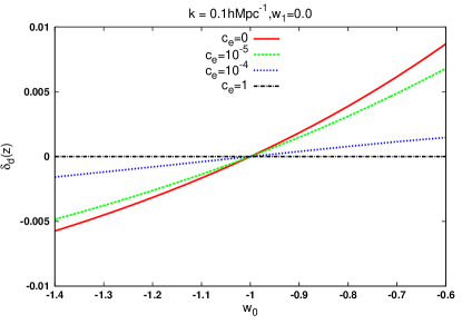
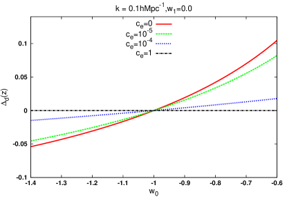
DE perturbations not only depend on the sound speed but also on the EoS wdsubscript๐‘คdw_{\rm d}. In the limit wdโ†’โˆ’1โ†’subscript๐‘คd1w_{\rm d}\rightarrow-1 all DE perturbations are washed out due to the 1+wd1subscript๐‘คd1+w_{\rm d} factor in front of the source term in the evolution equation of ฮดdsubscript๐›ฟd\delta_{\rm d}. To show how the DE sound speed affects the linear evolution of DM, we consider ฮฉm=0.28subscriptฮฉ๐‘š0.28\Omega_{m}=0.28 and h=0.7โ„Ž0.7h=0.7 in the wCDM model to evaluate ฮดdsubscript๐›ฟd\delta_{\rm d} and ฮ”d=ฮดdฮดmsubscriptฮ”dsubscript๐›ฟdsubscript๐›ฟm\Delta_{\rm d}=\frac{\delta_{\rm d}}{\delta_{\rm m}}, the relative DE density contrast, for a few distinct values of the DE sound speed as a function of the EoS. In Fig.ย (1) the density contrast of DE as a function of wdsubscript๐‘คdw_{\rm d} at the present time is presented. The non-clustering case remains homogeneous but for small values of the DE sound speed, the density contrast grows while increasing the EoS. In contrast to the non-clustering case, the fully clustering regime with ce=0subscript๐‘e0c_{\rm e}=0 gives a maximum value for the DE density contrast. In Fig.ย (2) the relative DE density contrast is shown as a function of EoS. The behaviour of this quantity is similar to that of the density contrast.
Refer to caption
Figure 1: The density contrast of DE as a function of the EoS at the present time for four different values of the sound speed. The red solid curve shows a fully clustering DE model with ce=0subscript๐‘e0c_{\rm e}=0. The green dashed (blue dotted) curve is for ce=10โˆ’5subscript๐‘esuperscript105c_{\rm e}=10^{-5} (ce=10โˆ’4subscript๐‘esuperscript104c_{\rm e}=10^{-4}). A non-clustering model with ce=1subscript๐‘๐‘’1c_{e}=1 is shown by a black dashed-dotted line.
Refer to caption
Figure 2: The relative density contrast of DE as a function of the EoS at the present time for four different values of the sound speed. Line style and colours are as in Fig.ย (1).

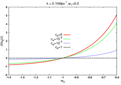
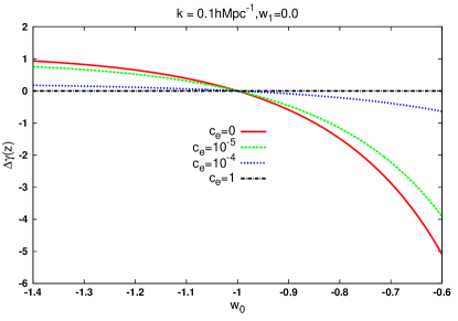
As we stated the quantity fโ€‹ฯƒ8โ€‹(z)๐‘“subscript๐œŽ8๐‘งf\sigma_{8}(z) is affected by DE clustering. To show how fโ€‹ฯƒ8โ€‹(z)๐‘“subscript๐œŽ8๐‘งf\sigma_{8}(z) changes with the DE sound speed, we evaluate ฮ”โ€‹fโ€‹ฯƒ8โ€‹(z)=fhโ€‹ฯƒ8,hโ€‹(z)โˆ’fโ€‹ฯƒ8โ€‹(z)fโ€‹ฯƒ8โ€‹(z)ร—100ฮ”๐‘“subscript๐œŽ8๐‘งsubscript๐‘“โ„Žsubscript๐œŽ8โ„Ž๐‘ง๐‘“subscript๐œŽ8๐‘ง๐‘“subscript๐œŽ8๐‘ง100\Delta f\sigma_{8}(z)=\frac{f_{h}\sigma_{8,h}(z)-f\sigma_{8}(z)}{f\sigma_{8}(z)}\times 100 and ฮ”โ€‹ฮณโ€‹(z)=ฮณhโ€‹(z)โˆ’ฮณโ€‹(z)ฮณโ€‹(z)ร—100ฮ”๐›พ๐‘งsubscript๐›พโ„Ž๐‘ง๐›พ๐‘ง๐›พ๐‘ง100\Delta\gamma(z)=\frac{\gamma_{h}(z)-\gamma(z)}{\gamma(z)}\times 100 as a function of the EoS parameter. In the previous equations, hโ„Žh stands for homogeneous DE. For the growth rate, results at present time are presented in Fig.ย (3). As expected, the deviation increases by increasing the EoS and for wd<โˆ’0.9subscript๐‘คd0.9w_{\rm d}<-0.9 the difference is less than 1%percent11\%. The relative difference between homogeneous and clustering DE for the growth index ฮ”โ€‹ฮณโ€‹(z=0)ฮ”๐›พ๐‘ง0\Delta\gamma(z=0) has been shown in Fig.ย (4). The difference between the homogeneous and the clustering DE models is also very small for wdsubscript๐‘คdw_{\rm d} very close to the ฮ›ฮ›\LambdaCDM model.

Refer to caption
Figure 3: The relative difference of fโ€‹ฯƒ8๐‘“subscript๐œŽ8f\sigma_{8} at the present time as a function of EoS. Line style and colours are as in Fig.ย (1).
Refer to caption
Figure 4: The relative difference of the growth index at present time as a function of EoS. Line style and colours are as in Fig.ย (1).

3 Observational constraints on the dark energy sound speed

In this section we use current available observational data sets to constrain the cosmological background parameters and the DE sound speed. In this analysis we assume that the DE sound speed is constant in time, regardless of the particular equation-of-state parameter adopted. Our cosmological model will be described by the following parameters: ฮฉm0subscriptฮฉm0\Omega_{\rm m0} (matter density), ฮฉb0subscriptฮฉb0\Omega_{\rm b0} (baryon density), h=H0/100โ„Žsubscript๐ป0100h=H_{0}/100 (normalised Hubble constant), w0subscript๐‘ค0w_{0} and w1subscript๐‘ค1w_{1} (dark energy equation-of-state parameters) and cesubscript๐‘ec_{\rm e} (effective sound speed) to describe the dark energy perturbations. In our analysis we assume a flat universe so that ฮฉDM+ฮฉb+ฮฉd=1subscriptฮฉDMsubscriptฮฉbsubscriptฮฉd1\Omega_{\rm DM}+\Omega_{\rm b}+\Omega_{\rm d}=1, hence the amount of dark energy is known from the knowledge of the matter and baryon density parameters.

The first data set we consider is the SnIa distance module from Union 2.1 sample (Suzuki etย al., 2012). This data set includes 580 SnIa and its ฯ‡2superscript๐œ’2\chi^{2} is given by:

ฯ‡sn2=โˆ‘i[ฮผthโ€‹(zi)โˆ’ฮผobโ€‹(zi)]2ฯƒi2,subscriptsuperscript๐œ’2snsubscript๐‘–superscriptdelimited-[]subscript๐œ‡thsubscript๐‘ง๐‘–subscript๐œ‡obsubscript๐‘ง๐‘–2superscriptsubscript๐œŽ๐‘–2\chi^{2}_{\rm sn}=\sum_{i}\frac{[\mu_{\rm th}(z_{i})-\mu_{\rm ob}(z_{i})]^{2}}{\sigma_{i}^{2}}\;, (18)

where ฮผthโ€‹(z)=5โ€‹log10โก[(1+z)โ€‹โˆซ0zdโ€‹xEโ€‹(x)]+ฮผ0subscript๐œ‡th๐‘ง5subscript101๐‘งsuperscriptsubscript0๐‘ง๐‘‘๐‘ฅ๐ธ๐‘ฅsubscript๐œ‡0\mu_{\rm th}(z)=5\log_{10}\left[(1+z)\int_{0}^{z}\frac{dx}{E(x)}\right]+\mu_{0}, ฮผ0=42.384โˆ’5โ€‹log10โกhsubscript๐œ‡042.3845subscript10โ„Ž\mu_{0}=42.384-5\log_{10}h and ฯƒisubscript๐œŽ๐‘–\sigma_{i} are the corresponding uncertainties. Before finding the minimum of ฯ‡sn2subscriptsuperscript๐œ’2sn\chi^{2}_{\rm sn} we can expand ฯ‡sn2subscriptsuperscript๐œ’2sn\chi^{2}_{\rm sn} around ฮผ0subscript๐œ‡0\mu_{0}

ฯ‡sn2=A+2โ€‹Bโ€‹ฮผ0+Cโ€‹ฮผ02,subscriptsuperscript๐œ’2sn๐ด2๐ตsubscript๐œ‡0๐ถsuperscriptsubscript๐œ‡02\chi^{2}_{\rm sn}=A+2B\mu_{0}+C\mu_{0}^{2}\;, (19)

where

A๐ด\displaystyle A =\displaystyle= โˆ‘i[ฮผthโ€‹(ฮผ0=0)โˆ’ฮผob]2ฯƒi2,subscript๐‘–superscriptdelimited-[]subscript๐œ‡thsubscript๐œ‡00subscript๐œ‡ob2superscriptsubscript๐œŽ๐‘–2\displaystyle\sum_{i}\frac{[\mu_{\rm th}(\mu_{0}=0)-\mu_{\rm ob}]^{2}}{\sigma_{i}^{2}}\;,
B๐ต\displaystyle B =\displaystyle= โˆ‘i[ฮผthโ€‹(ฮผ0=0)โˆ’ฮผob]ฯƒi2,subscript๐‘–delimited-[]subscript๐œ‡thsubscript๐œ‡00subscript๐œ‡obsuperscriptsubscript๐œŽ๐‘–2\displaystyle\sum_{i}\frac{[\mu_{\rm th}(\mu_{0}=0)-\mu_{\rm ob}]}{\sigma_{i}^{2}}\;,
C๐ถ\displaystyle C =\displaystyle= โˆ‘i1ฯƒi2.subscript๐‘–1superscriptsubscript๐œŽ๐‘–2\displaystyle\sum_{i}\frac{1}{\sigma_{i}^{2}}\;.

Obviously, for ฮผ0=โˆ’B/Csubscript๐œ‡0๐ต๐ถ\mu_{0}=-B/C Eq.ย (19) has a minimum, namely Aโˆ’B2C๐ดsuperscript๐ต2๐ถA-\frac{B^{2}}{C}. Now by defining ฯ‡~sn2=Aโˆ’B2Csuperscriptsubscript~๐œ’sn2๐ดsuperscript๐ต2๐ถ\tilde{\chi}_{\rm sn}^{2}=A-\frac{B^{2}}{C}, we can use the minimum of ฯ‡~sn2superscriptsubscript~๐œ’sn2\tilde{\chi}_{\rm sn}^{2} which is independent of ฮผ0subscript๐œ‡0\mu_{0} in order to find the best values of the parameters. Of course both estimators provide the same results (Nesseris & Perivolaropoulos, 2005).

The second data set we consider is the BAO sample which includes 6 distinct measurements of the baryon acoustic scale. These 6 data points and their references are summarised in Tab.ย (LABEL:tab:bao).

Table 1: The current available BAO data which we use in our analysis.
z๐‘งz disubscript๐‘‘๐‘–d_{i} Survey & References
0.1060.1060.106 0.3360.3360.336 6dF (Beutler etย al., 2011)
0.350.350.35 0.1130.1130.113 SDSS-DR7 (Padmanabhan etย al., 2012)
0.570.570.57 0.0730.0730.073 SDSS-DR9 (Anderson etย al., 2013)
0.440.440.44 0.09160.09160.0916 WiggleZ (Blake etย al., 2011)
0.60.60.6 0.07260.07260.0726 WiggleZ (Blake etย al., 2011)
0.730.730.73 0.05920.05920.0592 WiggleZ (Blake etย al., 2011)

To find the ฯ‡BAO2subscriptsuperscript๐œ’2BAO\chi^{2}_{\rm BAO} we follow the same procedure as Hinshaw etย al. (2013). So the ฯ‡BAO2subscriptsuperscript๐œ’2BAO\chi^{2}_{\rm BAO} is given by

ฯ‡BAO2=๐˜Tโ€‹๐‚BAOโˆ’1โ€‹๐˜,subscriptsuperscript๐œ’2BAOsuperscript๐˜๐‘‡superscriptsubscript๐‚BAO1๐˜\chi^{2}_{\rm BAO}=\mathbf{Y}^{T}\mathbf{C}_{\rm BAO}^{-1}\mathbf{Y}\;, (20)

where ๐˜=(dโ€‹(0.1)โˆ’d1,1dโ€‹(0.35)โˆ’1d2,1dโ€‹(0.57)โˆ’1d3,dโ€‹(0.44)โˆ’d4,dโ€‹(0.6)โˆ’d5,dโ€‹(0.73)โˆ’d6)๐˜๐‘‘0.1subscript๐‘‘11๐‘‘0.351subscript๐‘‘21๐‘‘0.571subscript๐‘‘3๐‘‘0.44subscript๐‘‘4๐‘‘0.6subscript๐‘‘5๐‘‘0.73subscript๐‘‘6\mathbf{Y}=(d(0.1)-d_{1},\frac{1}{d(0.35)}-\frac{1}{d_{2}},\frac{1}{d(0.57)}-\frac{1}{d_{3}},d(0.44)-d_{4},d(0.6)-d_{5},d(0.73)-d_{6}) and

dโ€‹(z)=rsโ€‹(zdrag)DVโ€‹(z),๐‘‘๐‘งsubscript๐‘Ÿssubscript๐‘งdragsubscript๐ท๐‘‰๐‘งd(z)=\frac{r_{\rm s}(z_{\rm drag})}{D_{V}(z)}\;, (21)

with

rsโ€‹(a)=โˆซ0acsโ€‹dโ€‹aa2โ€‹Hโ€‹(a),subscript๐‘Ÿs๐‘Žsuperscriptsubscript0๐‘Žsubscript๐‘s๐‘‘๐‘Žsuperscript๐‘Ž2๐ป๐‘Žr_{\rm s}(a)=\int_{0}^{a}\frac{c_{\rm s}da}{a^{2}H(a)}\;, (22)

is the comoving sound horizon at the baryon drag epoch, cssubscript๐‘sc_{\rm s} the baryon sound speed and DVโ€‹(z)subscript๐ท๐‘‰๐‘งD_{V}(z) is defined by:

DVโ€‹(z)=[(1+z)2โ€‹DA2โ€‹(z)โ€‹zHโ€‹(z)]13,subscript๐ท๐‘‰๐‘งsuperscriptdelimited-[]superscript1๐‘ง2subscriptsuperscript๐ท2A๐‘ง๐‘ง๐ป๐‘ง13D_{V}(z)=\left[(1+z)^{2}D^{2}_{\rm A}(z)\frac{z}{H(z)}\right]^{\frac{1}{3}}\;, (23)

and DAโ€‹(z)subscript๐ทA๐‘งD_{\rm A}(z) is the angular diameter distance. We used the fitting formula for zdsubscript๐‘งdz_{\rm d} from Eisenstein & Hu (1998) and the baryon sound speed is given by:

csโ€‹(a)=13โ€‹(1+3โ€‹ฮฉb04โ€‹ฮฉฮณ0โ€‹a),subscript๐‘s๐‘Ž1313superscriptsubscriptฮฉ๐‘04superscriptsubscriptฮฉ๐›พ0๐‘Žc_{\rm s}(a)=\frac{1}{\sqrt{3(1+\frac{3\Omega_{b}^{0}}{4\Omega_{\gamma}^{0}}a)}}\;, (24)

where we set ฮฉฮณ0=2.469ร—10โˆ’5โ€‹hโˆ’2superscriptsubscriptฮฉ๐›พ02.469superscript105superscriptโ„Ž2\Omega_{\gamma}^{0}=2.469\times 10^{-5}h^{-2} (Hinshaw etย al., 2013). The covariance matrix ๐‚BAOโˆ’1superscriptsubscript๐‚BAO1\mathbf{C}_{\rm BAO}^{-1} in Eq.ย (20) was obtained by Hinshaw etย al. (2013)

(4444.40.0.0.0.0.0.34.6020.0.0.0.0.0.20.66110.0.0.0.0.0.24532.1โˆ’25137.712099.10.0.0.โˆ’25137.7134598.4โˆ’64783.90.0.0.12099.1โˆ’64783.9128837.6).4444.400000034.60200000020.661100000024532.125137.712099.100025137.7134598.464783.900012099.164783.9128837.6\displaystyle\left(\begin{array}[]{cccccc}4444.4&0.&0.&0.&0.&0.\\ 0.&34.602&0.&0.&0.&0.\\ 0.&0.&20.6611&0.&0.&0.\\ 0.&0.&0.&24532.1&-25137.7&12099.1\\ 0.&0.&0.&-25137.7&134598.4&-64783.9\\ 0.&0.&0.&12099.1&-64783.9&128837.6\end{array}\right)\;. (31)

The position of the CMB acoustic peak provides a useful data to constrain dark energy models. The position of this peak is given by (la,R,zโˆ—)subscript๐‘™a๐‘…subscript๐‘งโˆ—(l_{\rm a},R,z_{\ast}), where R๐‘…R is the scale distance to recombination

lasubscript๐‘™๐‘Ž\displaystyle l_{a} =\displaystyle= ฯ€โ€‹DAโ€‹(zโˆ—)rsโ€‹(zโˆ—),๐œ‹subscript๐ทAsubscript๐‘งโˆ—subscript๐‘Ÿ๐‘ subscript๐‘งโˆ—\displaystyle\pi\frac{D_{\rm A}(z_{\ast})}{r_{s}(z_{\ast})}\;, (32)
R๐‘…\displaystyle R =\displaystyle= ฮฉm0โ€‹H0โ€‹DAโ€‹(zโˆ—),superscriptsubscriptฮฉm0subscript๐ป0subscript๐ทAsubscript๐‘งโˆ—\displaystyle\sqrt{\Omega_{\rm m}^{0}}H_{\rm 0}D_{\rm A}(z_{\ast})\;, (33)

and rsโ€‹(z)subscript๐‘Ÿs๐‘งr_{\rm s}(z) is the comoving sound horizon defined in Eq.ย (22). In this case we used the formula for zโˆ—subscript๐‘งโˆ—z_{\ast} from Hu & Sugiyama (1996). For the WMAP data set we have (Hinshaw etย al., 2013)

๐—CMB=(laโˆ’302.40Rโˆ’1.7264zโˆ—โˆ’1090.88),subscript๐—CMBsubscript๐‘™a302.40๐‘…1.7264subscript๐‘งโˆ—1090.88\mathbf{X}_{\rm CMB}=\left(\begin{array}[]{c}l_{\rm a}-302.40\\ R-1.7264\\ z_{\ast}-1090.88\end{array}\right)\;, (34)

and

๐‚CMBโˆ’1=(3.18218.253โˆ’1.42918.25311887.879โˆ’193.808โˆ’1.429โˆ’193.8084.556).superscriptsubscript๐‚CMB13.18218.2531.42918.25311887.879193.8081.429193.8084.556\displaystyle\mathbf{C}_{\rm CMB}^{-1}=\left(\begin{array}[]{ccc}3.182&18.253&-1.429\\ 18.253&11887.879&-193.808\\ -1.429&-193.808&4.556\end{array}\right)\;. (38)

In addition to this data set the Planck data provide more accurate CMB data for which the position of the acoustic peak is given by (Shafer & Huterer, 2014)

๐—CMB=(laโˆ’301.65Rโˆ’1.7499zโˆ—โˆ’1090.41),subscript๐—CMBsubscript๐‘™a301.65๐‘…1.7499subscript๐‘งโˆ—1090.41\mathbf{X}_{\rm CMB}=\left(\begin{array}[]{c}l_{\rm a}-301.65\\ R-1.7499\\ z_{\ast}-1090.41\end{array}\right)\;, (39)

and

๐‚CMBโˆ’1=(42.7044โˆ’418.36โˆ’0.7820โˆ’418.3657366.3โˆ’762.152โˆ’0.7820โˆ’762.15214.6995).superscriptsubscript๐‚CMB142.7044418.360.7820418.3657366.3762.1520.7820762.15214.6995\displaystyle\mathbf{C}_{\rm CMB}^{-1}=\left(\begin{array}[]{ccc}42.7044&-418.36&-0.7820\\ -418.36&57366.3&-762.152\\ -0.7820&-762.152&14.6995\end{array}\right)\;. (43)

In both cases the ฯ‡CMB2subscriptsuperscript๐œ’2CMB\chi^{2}_{\rm CMB} is given by :

ฯ‡CMB2=๐—CMBTโ€‹๐‚CMBโˆ’1โ€‹๐—CMB.subscriptsuperscript๐œ’2CMBsuperscriptsubscript๐—CMB๐‘‡superscriptsubscript๐‚CMB1subscript๐—CMB\chi^{2}_{\rm CMB}=\mathbf{X}_{\rm CMB}^{T}\mathbf{C}_{\rm CMB}^{-1}\mathbf{X}_{\rm CMB}\;. (44)

A further data set used in this work is the Hubble evolution data obtained from the evolution of galaxies (Simon etย al., 2005). We use the 12 available data points and the ฯ‡2superscript๐œ’2\chi^{2} for this data set is:

ฯ‡H2=โˆ‘i[Hโ€‹(zi)โˆ’Hob,i]2ฯƒi2.subscriptsuperscript๐œ’2Hsubscript๐‘–superscriptdelimited-[]๐ปsubscript๐‘ง๐‘–subscript๐ปobi2superscriptsubscript๐œŽ๐‘–2\chi^{2}_{\rm H}=\sum_{i}\frac{[H(z_{i})-H_{\rm ob,i}]^{2}}{\sigma_{i}^{2}}\;. (45)

The Big Bang Nucleosynthesis (BBN) provides a data point (Serra etย al., 2009; Burles etย al., 2001) which constrains mostly ฮฉb0superscriptsubscriptฮฉb0\Omega_{\rm b}^{0}. The ฯ‡BBN2subscriptsuperscript๐œ’2BBN\chi^{2}_{\rm BBN} is given by

ฯ‡BBN2=(ฮฉb0โ€‹h2โˆ’0.022)20.0022.subscriptsuperscript๐œ’2BBNsuperscriptsuperscriptsubscriptฮฉb0superscriptโ„Ž20.0222superscript0.0022\chi^{2}_{\rm BBN}=\frac{(\Omega_{\rm b}^{0}h^{2}-0.022)^{2}}{0.002^{2}}\;. (46)

The final data set used is the growth rate data. These data were derived from redshift space distortions from galaxy surveys including PSCs, 2DF, VVDS, SDSS, 6dF, 2MASS, BOSS and WiggleZ and the data with their references are shown in Tab.ย 2. We solve Eqs.ย (10) andย (11) numerically to find fโ€‹(z)โ€‹ฯƒ8โ€‹(z)๐‘“๐‘งsubscript๐œŽ8๐‘งf(z)\sigma_{8}(z) and compute ฯ‡fs2subscriptsuperscript๐œ’2fs\chi^{2}_{\rm fs} with

ฯ‡fs2=โˆ‘i[fโ€‹ฯƒ8โ€‹(zi)โˆ’fโ€‹ฯƒ8,ob]2ฯƒi2.subscriptsuperscript๐œ’2fssubscript๐‘–superscriptdelimited-[]๐‘“subscript๐œŽ8subscript๐‘ง๐‘–๐‘“subscript๐œŽ8ob2superscriptsubscript๐œŽ๐‘–2\chi^{2}_{\rm fs}=\sum_{i}\frac{[f\sigma_{8}(z_{i})-f\sigma_{8,\rm ob}]^{2}}{\sigma_{i}^{2}}\;. (47)
Table 2: The fโ€‹ฯƒ8โ€‹(z)๐‘“subscript๐œŽ8๐‘งf\sigma_{8}(z) data points including their references and surveys.
z fโ€‹ฯƒ8โ€‹(z)๐‘“subscript๐œŽ8๐‘งf\sigma_{8}(z) Reference
0.020.020.02 0.360ยฑ0.040plus-or-minus0.3600.0400.360\pm 0.040 Hudson & Turnbull (2013)
0.0670.0670.067 0.423ยฑ0.055plus-or-minus0.4230.0550.423\pm 0.055 Beutler etย al. (2012)
0.100.100.10 0.37ยฑ0.13plus-or-minus0.370.130.37\pm 0.13 Feix etย al. (2015)
0.170.170.17 0.510ยฑ0.060plus-or-minus0.5100.0600.510\pm 0.060 Percival etย al. (2004)
0.350.350.35 0.440ยฑ0.050plus-or-minus0.4400.0500.440\pm 0.050 Song & Percival (2009); Tegmark etย al. (2006)
0.770.770.77 0.490ยฑ0.180plus-or-minus0.4900.1800.490\pm 0.180 Guzzo etย al. (2008); Song & Percival (2009)
0.250.250.25 0.351ยฑ0.058plus-or-minus0.3510.0580.351\pm 0.058 Samushia etย al. (2012)
0.370.370.37 0.460ยฑ0.038plus-or-minus0.4600.0380.460\pm 0.038 Samushia etย al. (2012)
0.220.220.22 0.420ยฑ0.070plus-or-minus0.4200.0700.420\pm 0.070 Blake etย al. (2011)
0.410.410.41 0.450ยฑ0.040plus-or-minus0.4500.0400.450\pm 0.040 Blake etย al. (2011)
0.600.600.60 0.430ยฑ0.040plus-or-minus0.4300.0400.430\pm 0.040 Blake etย al. (2011)
0.600.600.60 0.433ยฑ0.067plus-or-minus0.4330.0670.433\pm 0.067 Tojeiro etย al. (2012)
0.780.780.78 0.380ยฑ0.040plus-or-minus0.3800.0400.380\pm 0.040 Blake etย al. (2011)
0.570.570.57 0.427ยฑ0.066plus-or-minus0.4270.0660.427\pm 0.066 Reid etย al. (2012)
0.300.300.30 0.407ยฑ0.055plus-or-minus0.4070.0550.407\pm 0.055 Tojeiro etย al. (2012)
0.400.400.40 0.419ยฑ0.041plus-or-minus0.4190.0410.419\pm 0.041 Tojeiro etย al. (2012)
0.500.500.50 0.427ยฑ0.043plus-or-minus0.4270.0430.427\pm 0.043 Tojeiro etย al. (2012)
0.800.800.80 0.47ยฑ0.08plus-or-minus0.470.080.47\pm 0.08 deย la Torre etย al. (2013)

The overall likelihood function is given by the product of the individual likelihoods:

โ„’tot=โ„’snร—โ„’BAOร—โ„’CMBร—โ„’Hร—โ„’BBNร—โ„’fs,subscriptโ„’totsubscriptโ„’snsubscriptโ„’BAOsubscriptโ„’CMBsubscriptโ„’๐ปsubscriptโ„’BBNsubscriptโ„’fs{\cal L}_{\rm tot}={\cal L}_{\rm sn}\times{\cal L}_{\rm BAO}\times{\cal L}_{\rm CMB}\times{\cal L}_{H}\times{\cal L}_{\rm\rm BBN}\times{\cal L}_{\rm fs}\;, (48)

and the total chi-square ฯ‡tot2subscriptsuperscript๐œ’2tot\chi^{2}_{\rm tot} is given by:

ฯ‡tot2=ฯ‡sn2+ฯ‡BAO2+ฯ‡CMB2+ฯ‡H2+ฯ‡BBN2+ฯ‡fs2.subscriptsuperscript๐œ’2totsubscriptsuperscript๐œ’2snsubscriptsuperscript๐œ’2BAOsubscriptsuperscript๐œ’2CMBsubscriptsuperscript๐œ’2๐ปsubscriptsuperscript๐œ’2BBNsubscriptsuperscript๐œ’2fs\chi^{2}_{\rm tot}=\chi^{2}_{\rm sn}+\chi^{2}_{\rm BAO}+\chi^{2}_{\rm CMB}+\chi^{2}_{H}+\chi^{2}_{\rm BBN}+\chi^{2}_{\rm fs}\;. (49)
Table 3: The best value parameters and their 1-ฯƒ๐œŽ\sigma uncertainty for the wCDM model.
Parameters Best (WMAP) Best (Planck)
hโ„Žh 0.6955โˆ’0.0037+0.0040subscriptsuperscript0.69550.00400.00370.6955^{+0.0040}_{-0.0037} 0.7064โˆ’0.0012+0.0011subscriptsuperscript0.70640.00110.00120.7064^{+0.0011}_{-0.0012}
ฮฉDM0superscriptsubscriptฮฉDM0\Omega_{\rm DM}^{0} 0.2273โˆ’0.0029+0.0027subscriptsuperscript0.22730.00270.00290.2273^{+0.0027}_{-0.0029} 0.2361โˆ’0.0010+0.0010subscriptsuperscript0.23610.00100.00100.2361^{+0.0010}_{-0.0010}
ฮฉb0superscriptsubscriptฮฉb0\Omega_{\rm b}^{0} 0.0470โˆ’0.0005+0.0004subscriptsuperscript0.04700.00040.00050.0470^{+0.0004}_{-0.0005} 0.0482โˆ’0.0002+0.0003subscriptsuperscript0.04820.00030.00020.0482^{+0.0003}_{-0.0002}
w0subscript๐‘ค0w_{0} โˆ’0.9436โˆ’0.0141+0.0144subscriptsuperscript0.94360.01440.0141-0.9436^{+0.0144}_{-0.0141} โˆ’0.9975โˆ’0.0053+0.0055subscriptsuperscript0.99750.00550.0053-0.9975^{+0.0055}_{-0.0053}
cesubscript๐‘ec_{\rm e} 0.00. 0.0010.0010.001
ฯƒ8subscript๐œŽ8\sigma_{\rm 8} 0.8370.8370.837 0.8290.8290.829
Table 4: The best value parameters and their 1-ฯƒ๐œŽ\sigma uncertainty for the w(t)CDM model.
Parameters Best (WMAP) Best (Planck)
hโ„Žh 0.7001โˆ’0.0038+0.0040subscriptsuperscript0.70010.00400.00380.7001^{+0.0040}_{-0.0038} 0.7070โˆ’0.0013+0.0012subscriptsuperscript0.70700.00120.00130.7070^{+0.0012}_{-0.0013}
ฮฉDM0superscriptsubscriptฮฉDM0\Omega_{\rm DM}^{0} 0.2234โˆ’0.0027+0.0028subscriptsuperscript0.22340.00280.00270.2234^{+0.0028}_{-0.0027} 0.2361โˆ’0.0011+0.0012subscriptsuperscript0.23610.00120.00110.2361^{+0.0012}_{-0.0011}
ฮฉb0superscriptsubscriptฮฉb0\Omega_{\rm b}^{0} 0.0474โˆ’0.0005+0.0005subscriptsuperscript0.04740.00050.00050.0474^{+0.0005}_{-0.0005} 0.0481โˆ’0.0003+0.0003subscriptsuperscript0.04810.00030.00030.0481^{+0.0003}_{-0.0003}
w0subscript๐‘ค0w_{0} โˆ’1.0176โˆ’0.0124+0.0128subscriptsuperscript1.01760.01280.0124-1.0176^{+0.0128}_{-0.0124} โˆ’0.95204โˆ’0.0058+0.0060subscriptsuperscript0.952040.00600.0058-0.95204^{+0.0060}_{-0.0058}
w1subscript๐‘ค1w_{1} 0.3289โˆ’0.0405+0.0395subscriptsuperscript0.32890.03950.04050.3289^{+0.0395}_{-0.0405} โˆ’0.18512โˆ’0.0195+0.0205subscriptsuperscript0.185120.02050.0195-0.18512^{+0.0205}_{-0.0195}
cesubscript๐‘ec_{\rm e} 0.0020.0020.002 0.00.
ฯƒ8subscript๐œŽ8\sigma_{\rm 8} 0.8400.8400.840 0.8290.8290.829

We calculate the total chi-square ฯ‡tot2subscriptsuperscript๐œ’2tot\chi^{2}_{\rm tot} and find the best value of the parameters with an MCMC algorithm. The number of degrees of freedom is ฮฝ=Nโˆ’nfitโˆ’1๐œˆ๐‘subscript๐‘›fit1\nu=N-n_{\rm fit}-1, where N=616๐‘616N=616 and nfitsubscript๐‘›fitn_{\rm fit} is the number of the fitted parameters. The results of this analysis for the wCDM, w(t)CDM and ฮ›ฮ›\LambdaCDM are summarized in Tabs.ย (3),ย (4) andย (5) respectively.

Table 5: The best value parameters and their 1-ฯƒ๐œŽ\sigma uncertainty for the ฮ›ฮ›\LambdaCDM model.
Parameters Best (WMAP) Best (Planck)
hโ„Žh 0.7048โˆ’0.0041+0.0042subscriptsuperscript0.70480.00420.00410.7048^{+0.0042}_{-0.0041} 0.7069โˆ’0.0010+0.0011subscriptsuperscript0.70690.00110.00100.7069^{+0.0011}_{-0.0010}
ฮฉDM0superscriptsubscriptฮฉDM0\Omega_{\rm DM}^{0} 0.2261โˆ’0.0029+0.0030subscriptsuperscript0.22610.00300.00290.2261^{+0.0030}_{-0.0029} 0.2359โˆ’0.0011+0.0010subscriptsuperscript0.23590.00100.00110.2359^{+0.0010}_{-0.0011}
ฮฉb0superscriptsubscriptฮฉb0\Omega_{\rm b}^{0} 0.0456โˆ’0.0005+0.0006subscriptsuperscript0.04560.00060.00050.0456^{+0.0006}_{-0.0005} 0.0481โˆ’0.0003+0.0003subscriptsuperscript0.04810.00030.00030.0481^{+0.0003}_{-0.0003}
ฯƒ8subscript๐œŽ8\sigma_{\rm 8} 0.8390.8390.839 0.8290.8290.829

To compare the DE models we have computed the corrected Akaike information criterion (AIC) (Akaike, 1974; Sugiura, 1978) which, in our case, due to N/nfit>40๐‘subscript๐‘›fit40N/n_{\rm fit}>40, is given by:

AIC=ฯ‡mโ€‹iโ€‹n2+2โ€‹nfit.AICsubscriptsuperscript๐œ’2๐‘š๐‘–๐‘›2subscript๐‘›fit{\rm AIC}=\chi^{2}_{min}+2n_{\rm fit}\;. (50)

A smaller value of AIC indicates a better model-data fit. Of course it is well known that small differences in AIC are not necessarily significant and therefore, in order to assess the effectiveness of the different models in reproducing the data, we need to estimate the model pair difference ฮ”ฮ”\DeltaAIC=AICyโˆ’AICxabsentsubscriptAIC๐‘ฆsubscriptAIC๐‘ฅ={\rm AIC}_{y}-{\rm AIC}_{x}. The higher the value of |ฮ”โ€‹AIC|ฮ”AIC|\Delta{\rm AIC}|, the higher the evidence against the model with a higher value of AICAIC{\rm AIC}. With a difference |ฮ”|\DeltaAIC|โ‰ฅ2|\geq 2 indicating a positive evidence and |ฮ”|\DeltaAIC|โ‰ฅ6|\geq 6 indicating a strong evidence, while a value |ฮ”|\DeltaAIC|โ‰ค2|\leq 2 indicates consistency among the two models. The results of our analysis are the following:

  1. 1.

    Using WMAP data:

    • โ€ข

      For the wCDM model, ฯ‡min2=586.53subscriptsuperscript๐œ’2min586.53\chi^{2}_{\rm min}=586.53, nfit=5subscript๐‘›fit5n_{\rm fit}=5, so AIC=596.53

    • โ€ข

      For the w(t)CDM model, ฯ‡min2=585.32subscriptsuperscript๐œ’2min585.32\chi^{2}_{\rm min}=585.32, nfit=6subscript๐‘›fit6n_{\rm fit}=6, so AIC=597.32

    • โ€ข

      For the ฮ›ฮ›\LambdaCDM model, ฯ‡min2=589.22subscriptsuperscript๐œ’2min589.22\chi^{2}_{\rm min}=589.22, nfit=3subscript๐‘›fit3n_{\rm fit}=3, so AIC=595.32

  2. 2.

    Using Planck data:

    • โ€ข

      For the wCDM model, ฯ‡min2=595.76subscriptsuperscript๐œ’2min595.76\chi^{2}_{\rm min}=595.76, nfit=5subscript๐‘›fit5n_{\rm fit}=5, so AIC=605.76

    • โ€ข

      For the w(t)CDM model, ฯ‡min2=595.50subscriptsuperscript๐œ’2min595.50\chi^{2}_{\rm min}=595.50, nfit=6subscript๐‘›fit6n_{\rm fit}=6, so AIC=607.50

    • โ€ข

      For the ฮ›ฮ›\LambdaCDM model, ฯ‡min2=595.79subscriptsuperscript๐œ’2min595.79\chi^{2}_{\rm min}=595.79, nfit=3subscript๐‘›fit3n_{\rm fit}=3, so AIC=601.79

Concerning the best value of the dark energy sound speed we find that it tends to zero but the corresponding error bars remain quite large within 1โ€‹ฯƒ1๐œŽ1\sigma. In particular cesubscript๐‘ec_{\rm e} lies in the range โˆˆ[0.,1]\in[0.,1].

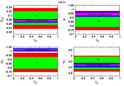
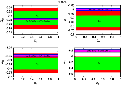
In order to investigate the range of validity for cesubscript๐‘ec_{\rm e}, in Figs.ย (5) and (6) we provide the 1โ€‹ฯƒ1๐œŽ1\sigma and 2โ€‹ฯƒ2๐œŽ2\sigma contours of our analysis. Note that in both plots the upper panels are for wCDM in which we present the confidence levels in the (ce,ฮฉm)subscript๐‘esubscriptฮฉm(c_{\rm e},\Omega_{\rm m}) and (ce,w)subscript๐‘e๐‘ค(c_{\rm e},w) planes, where ฮฉm=ฮฉDM0+ฮฉb0subscriptฮฉmsuperscriptsubscriptฮฉDM0superscriptsubscriptฮฉb0\Omega_{\rm m}=\Omega_{\rm DM}^{0}+\Omega_{\rm b}^{0}. In the bottom panels of Figs.ย (5) and (6) the contours for w0subscript๐‘ค0w_{0} and w1subscript๐‘ค1w_{1} in the CPL model are shown with respect to the DE sound speed. From this analysis it becomes clear that there is a strong degeneracy between cesubscript๐‘ec_{\rm e} and (ฮฉm,w)subscriptฮฉm๐‘ค(\Omega_{\rm m},w) which implies that all values in the interval 0โ‰คceโ‰ค10subscript๐‘e10\leq c_{\rm e}\leq 1 are acceptable within the 1โ€‹ฯƒ1๐œŽ1\sigma uncertainty. As we stated, with data used in this paper the error bar of DE sound speed is quite large.
Refer to caption
Figure 5: The 1โ€‹ฯƒ1๐œŽ1\sigma and 2โ€‹ฯƒ2๐œŽ2\sigma contours of ฮฉmsubscriptฮฉm\Omega_{\rm m}(wCDM), w๐‘คw(wCDM), w0subscript๐‘ค0w_{0}(w(t)CDM) and w1subscript๐‘ค1w_{1}(w(t)CDM) versus DE sound speed using WMAP data. The 1โ€‹ฯƒ1๐œŽ1\sigma and 2โ€‹ฯƒ2๐œŽ2\sigma contours correspond to ฯ‡2โˆ’ฯ‡b2=2.3superscript๐œ’2subscriptsuperscript๐œ’2b2.3\chi^{2}-\chi^{2}_{\rm b}=2.3 and ฯ‡2โˆ’ฯ‡b2=6.16superscript๐œ’2subscriptsuperscript๐œ’2b6.16\chi^{2}-\chi^{2}_{\rm b}=6.16. The green (red) area correspond to 1โ€‹ฯƒ1๐œŽ1\sigma (2โ€‹ฯƒ2๐œŽ2\sigma) using only fโ€‹ฯƒ8๐‘“subscript๐œŽ8f\sigma_{8} data and purple (blue) show 1โ€‹ฯƒ1๐œŽ1\sigma (2โ€‹ฯƒ2๐œŽ2\sigma) using all data set.
Refer to caption
Figure 6: Same as Fig.ย (5) but using the Planck shift parameter.

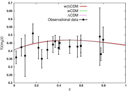
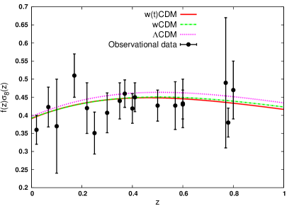
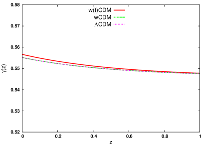
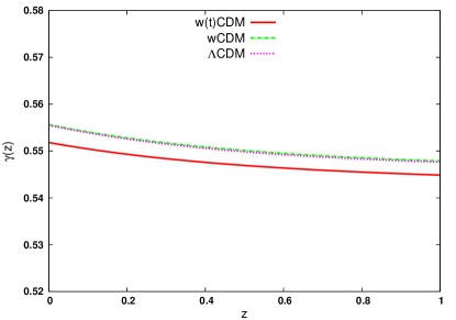
In Figs.ย (7) and (8) we present the quantity fโ€‹ฯƒ8โ€‹(z)๐‘“subscript๐œŽ8๐‘งf\sigma_{8}(z) for our best value parameters by considering the Planck and WMAP data for the wCDM, w(t)CDM and the ฮ›ฮ›\LambdaCDM models, respectively. We also show the observational data points. In addition to this quantity in Figs.ย (9) and (10) the growth index for the best values of the parameters have been shown. Note that using Planck CMB data our likelihood analysis indicates that all three models are very close to each others. 222See the results of ฯ‡2superscript๐œ’2\chi^{2} for the Planck case.

Refer to caption
Figure 7: The fโ€‹ฯƒ8โ€‹(z)๐‘“subscript๐œŽ8๐‘งf\sigma_{8}(z) quantity (using Planck data), for the best values cosmological parameters for the wCDM (green dot-dashed curve) and w(t)CDM (red solid curve) models. The ฮ›ฮ›\LambdaCDM model is shown by the violet short-dashed curve.
Refer to caption
Figure 8: The fโ€‹ฯƒ8โ€‹(z)๐‘“subscript๐œŽ8๐‘งf\sigma_{8}(z) quantity (using WMAP data), for the best values cosmological parameters for the wCDM (green dot-dashed curve) and w(t)CDM (red solid curve) models. The ฮ›ฮ›\LambdaCDM model is shown by the violet short-dashed curve.
Refer to caption
Figure 9: The growth index (using Planck data), for the best values cosmological parameters for the wCDM (green dot-dashed curve) and w(t)CDM (red solid curve) models. The ฮ›ฮ›\LambdaCDM model is shown by the violet short-dashed curve.
Refer to caption
Figure 10: The growth index (using WMAP data), for the best values cosmological parameters for the wCDM (green dot-dashed curve) and w(t)CDM (red solid curve) models. The ฮ›ฮ›\LambdaCDM model is shown by the violet short-dashed curve.

Previous works in literature tried to put constraints on the dark energy effective sound speed cesubscript๐‘ec_{\rm e} using different kind of data. deย Putter etย al. (2010)combination of CMB temperature power spectrum data, their cross-correlation with several mass-density tracers and the SDSS LRG auto-correlation function. Supernovae data were used to break degeneracies with background cosmological parameters. Hannestad (2005)set of Supernova data, LSS and CMB power spectra. Finally Xia etย al. (2008) performed a similar analysis for a single perfect fluid and a two-field Quintom dark energy model with w=โˆ’1๐‘ค1w=-1 crossing by analysing CMB anisotropy data, LSS and SNIa observational data. In all these studies, using a similar approach to the one used in this work, the authors reach our same results. While previous and current data can constrain at a good level the current equation-of-state parameter of the dark energy component, the quality of the observations is unfortunately still not sufficient enough to put any constraint on the dark energy effective sound speed. Note however that this is also due to the negligible contribution of dark energy at early times on one side, and to the fact that current observations favour wโ‰ƒโˆ’1similar-to-or-equals๐‘ค1w\simeq-1. As pointed out by deย Putter etย al. (2010), if one considers the case of early dark energy models (Doran & Robbers, 2006) where the contribution of dark energy at early times, i.e. CB, is not negligible, then more stringent limits can be set on cesubscript๐‘ec_{\rm e}.

4 Growth index analytic solution

In sectionย 2 we investigated the evolution of the growth index by solving numerically the system of Eqs.ย (5), (10) and (11). Here our aim is to extend the work of Basilakos (2015) in order to provide a general ฮณโ€‹(z)๐›พ๐‘ง\gamma(z) approximated solution which can be used in studies of structure formation. On sub-horizon scales, namely k2a2โ‰ซH2much-greater-thansuperscript๐‘˜2superscript๐‘Ž2superscript๐ป2\frac{k^{2}}{a^{2}}\gg H^{2} (or k2โ‰ซโ„‹2much-greater-thansuperscript๐‘˜2superscriptโ„‹2k^{2}\gg\mathcal{H}^{2}), Poisson equation (see appendixย B) takes the form

โˆ’k2a2โ€‹ฯ•=3โ€‹H22โ€‹[ฮฉmโ€‹ฮดm+ฮฉdโ€‹ฮดdโ€‹(1+3โ€‹ce)].superscript๐‘˜2superscript๐‘Ž2italic-ฯ•3superscript๐ป22delimited-[]subscriptฮฉmsubscript๐›ฟmsubscriptฮฉdsubscript๐›ฟd13subscript๐‘e-\frac{k^{2}}{a^{2}}\phi=\frac{3H^{2}}{2}\left[\Omega_{\rm m}\delta_{\rm m}+\Omega_{\rm d}\delta_{\rm d}(1+3c_{\rm e})\right]\;. (51)

Under the above conditions, Eq.ย (10) becomes

a2โ€‹d2โ€‹ฮดmdโ€‹a2+aโ€‹(3+Hห™H2)โ€‹dโ€‹ฮดmdโ€‹a=32โ€‹[ฮฉmโ€‹ฮดm+(1+3โ€‹ce)โ€‹ฮฉdโ€‹ฮดd].superscript๐‘Ž2superscript๐‘‘2subscript๐›ฟm๐‘‘superscript๐‘Ž2๐‘Ž3ห™๐ปsuperscript๐ป2๐‘‘subscript๐›ฟm๐‘‘๐‘Ž32delimited-[]subscriptฮฉmsubscript๐›ฟm13subscript๐‘esubscriptฮฉdsubscript๐›ฟda^{2}\frac{d^{2}\delta_{\rm m}}{da^{2}}+a\left(3+\frac{\dot{H}}{H^{2}}\right)\frac{d\delta_{\rm m}}{da}=\frac{3}{2}\left[\Omega_{\rm m}\delta_{\rm m}+(1+3c_{\rm e})\Omega_{\rm d}\delta_{\rm d}\right]\;. (52)

In this framework, for ฮดd=0subscript๐›ฟd0\delta_{\rm d}=0, the latter equation reduces to the well known scale independent equation which is also valid for the concordance ฮ›ฮ›\Lambda cosmology.

Concerning the equation of state parameter, it is well known that one can express it in terms of the Hubble parameter (Saini etย al., 2000; Huterer & Turner, 2001)

wdโ€‹(a)=โˆ’1โˆ’23โ€‹aโ€‹dโ€‹lnโกHdโ€‹a1โˆ’ฮฉmโ€‹(a),subscript๐‘คd๐‘Ž123๐‘Ž๐‘‘๐ป๐‘‘๐‘Ž1subscriptฮฉm๐‘Žw_{\rm d}(a)=\frac{-1-\frac{2}{3}a\frac{d\ln H}{da}}{1-\Omega_{\rm m}(a)}\;, (53)

or

aโ€‹dโ€‹lnโ€‹Hdโ€‹a=Hห™H2=โˆ’32โˆ’32โ€‹wdโ€‹(a)โ€‹ฮฉdโ€‹(a),๐‘Ž๐‘‘ln๐ป๐‘‘๐‘Žห™๐ปsuperscript๐ป23232subscript๐‘คd๐‘Žsubscriptฮฉd๐‘Ža\frac{d{\rm ln}H}{da}=\frac{{\dot{H}}}{H^{2}}=-\frac{3}{2}-\frac{3}{2}w_{\rm d}(a)\Omega_{\rm d}(a)\;, (54)

where ฮฉmโ€‹(a)=1โˆ’ฮฉdโ€‹(a)=ฮฉmโ€‹0a3โ€‹E2โ€‹(a)subscriptฮฉm๐‘Ž1subscriptฮฉd๐‘Žsubscriptฮฉ๐‘š0superscript๐‘Ž3superscript๐ธ2๐‘Ž\Omega_{\rm m}(a)=1-\Omega_{\rm d}(a)=\frac{\Omega_{m0}}{a^{3}E^{2}(a)} and Eโ€‹(a)=Hโ€‹(a)/H0๐ธ๐‘Ž๐ป๐‘Žsubscript๐ป0E(a)=H(a)/H_{0}. Now, substituting Eq.ย (54) and f=dโ€‹lnโ€‹ฮดm/dโ€‹lnโ€‹a๐‘“๐‘‘lnsubscript๐›ฟm๐‘‘ln๐‘Žf=d{\rm ln}\delta_{\rm m}/d{\rm ln}a into Eq.ย (52) we obtain the basic differential equation which governs the growth rate of clustering

aโ€‹dโ€‹fdโ€‹a+f2+(12โˆ’32โ€‹wdโ€‹ฮฉd)โ€‹f=32โ€‹[ฮฉm+(1+3โ€‹ce)โ€‹ฮ”dโ€‹ฮฉd],๐‘Ž๐‘‘๐‘“๐‘‘๐‘Žsuperscript๐‘“21232subscript๐‘คdsubscriptฮฉd๐‘“32delimited-[]subscriptฮฉm13subscript๐‘esubscriptฮ”dsubscriptฮฉda\frac{df}{da}+f^{2}+\left(\frac{1}{2}-\frac{3}{2}w_{\rm d}\Omega_{\rm d}\right)f=\frac{3}{2}\left[\Omega_{\rm m}+(1+3c_{\rm e})\Delta_{\rm d}\Omega_{\rm d}\right]\;, (55)

where ฮ”dโ€‹(a)โ‰กฮดd/ฮดmsubscriptฮ”d๐‘Žsubscript๐›ฟdsubscript๐›ฟm\Delta_{\rm d}(a)\equiv\delta_{\rm d}/\delta_{\rm m}. To this end, changing the variables in Eq.ย (55) from aโ€‹(z)๐‘Ž๐‘งa(z) to redshift [dโ€‹fdโ€‹a=โˆ’(1+z)โˆ’2โ€‹dโ€‹fdโ€‹z๐‘‘๐‘“๐‘‘๐‘Žsuperscript1๐‘ง2๐‘‘๐‘“๐‘‘๐‘ง\frac{df}{da}=-(1+z)^{-2}\frac{df}{dz}] and utilising fโ€‹(z)=ฮฉmโ€‹(z)ฮณโ€‹(z)๐‘“๐‘งsubscriptฮฉ๐‘šsuperscript๐‘ง๐›พ๐‘งf(z)=\Omega_{m}(z)^{\gamma(z)} we arrive to

โˆ’(1+z)โ€‹ฮณzโ€‹lnโ€‹(ฮฉm)+ฮฉmฮณ+3โ€‹wdโ€‹ฮฉdโ€‹(ฮณโˆ’12)+12=32โ€‹ฮฉm1โˆ’ฮณโ€‹X,1๐‘งsubscript๐›พ๐‘งlnsubscriptฮฉmsuperscriptsubscriptฮฉm๐›พ3subscript๐‘คdsubscriptฮฉd๐›พ121232superscriptsubscriptฮฉm1๐›พ๐‘‹-(1+z)\gamma_{z}{\rm ln}(\Omega_{\rm m})+\Omega_{\rm m}^{\gamma}+3w_{\rm d}\Omega_{\rm d}\left(\gamma-\frac{1}{2}\right)+\frac{1}{2}=\frac{3}{2}\Omega_{\rm m}^{1-\gamma}X\;, (56)

where ฮณz=dโ€‹ฮณ/dโ€‹zsubscript๐›พ๐‘ง๐‘‘๐›พ๐‘‘๐‘ง\gamma_{z}=d\gamma/dz and

Xโ€‹(z)=1+ฮฉdโ€‹(z)ฮฉmโ€‹(z)โ€‹ฮ”dโ€‹(z)โ€‹(1+3โ€‹ce).๐‘‹๐‘ง1subscriptฮฉd๐‘งsubscriptฮฉm๐‘งsubscriptฮ”d๐‘ง13subscript๐‘eX(z)=1+\frac{\Omega_{\rm d}(z)}{\Omega_{\rm m}(z)}\Delta_{\rm d}(z)(1+3c_{\rm e})\;. (57)

On the other hand, the parametrization fโ€‹(a)=dโ€‹lnโ€‹ฮดm/dโ€‹lnโ€‹aโ‰ƒฮฉmโ€‹(a)ฮณโ€‹(a)๐‘“๐‘Ž๐‘‘lnsubscript๐›ฟm๐‘‘ln๐‘Žsimilar-to-or-equalssubscriptฮฉ๐‘šsuperscript๐‘Ž๐›พ๐‘Žf(a)=d{\rm ln}\delta_{\rm m}/d{\rm ln}a\simeq\Omega_{m}(a)^{\gamma(a)} has a great impact in cosmological studies because it can be used in order to simplify the numerical calculations of Eq.ย (52). Obviously, a direct integration gives

ฮดmโ€‹(a,ฮณ)=aโ€‹(z)โ€‹expโ€‹[โˆซaiaโ€‹(z)dโ€‹uuโ€‹(ฮฉmฮณโ€‹(u)โˆ’1)],subscript๐›ฟm๐‘Ž๐›พ๐‘Ž๐‘งexpdelimited-[]superscriptsubscriptsubscript๐‘Ž๐‘–๐‘Ž๐‘ง๐‘‘๐‘ข๐‘ขsuperscriptsubscriptฮฉm๐›พ๐‘ข1\delta_{\rm m}(a,\gamma)=a(z)\;{\rm exp}\left[\int_{a_{i}}^{a(z)}\frac{du}{u}\;\left(\Omega_{\rm m}^{\gamma}(u)-1\right)\right]\;, (58)

where aโ€‹(z)=1/(1+z)๐‘Ž๐‘ง11๐‘งa(z)=1/(1+z) and aisubscript๐‘Ž๐‘–a_{i} is the scale factor of the universe at which the matter component dominates the cosmic fluid (here we use aiโ‰ƒ10โˆ’1similar-to-or-equalssubscript๐‘Ž๐‘–superscript101a_{i}\simeq 10^{-1} or ziโ‰ƒ10similar-to-or-equalssubscript๐‘ง๐‘–10z_{i}\simeq 10). Hence, the linear growth factor normalised to unity at the present epoch is Dโ€‹(a)=ฮดmโ€‹(a,ฮณ)ฮดmโ€‹(1,ฮณ)๐ท๐‘Žsubscript๐›ฟm๐‘Ž๐›พsubscript๐›ฟm1๐›พD(a)=\frac{\delta_{\rm m}(a,\gamma)}{\delta_{\rm m}(1,\gamma)}. Therefore, in order to proceed with the analysis we need to somehow know the functional form of ฮณโ€‹(z)๐›พ๐‘ง\gamma(z). From the phenomenological point of view we may parametrize ฮณโ€‹(z)๐›พ๐‘ง\gamma(z) as follows

ฮณโ€‹(z)=ฮณ0+ฮณ1โ€‹yโ€‹(z).๐›พ๐‘งsubscript๐›พ0subscript๐›พ1๐‘ฆ๐‘ง\gamma(z)=\gamma_{0}+\gamma_{1}y(z)\;. (59)

This equation can be seen as a first order Taylor expansion around some cosmological quantity such as aโ€‹(z)๐‘Ž๐‘งa(z) and z๐‘งz.

Recently, it has been found (Basilakos, 2012; Basilakos & Pouri, 2012, and references therein) that for those yโ€‹(z)๐‘ฆ๐‘งy(z) functions which satisfy the condition yโ€‹(0)=0๐‘ฆ00y(0)=0 [or ฮณโ€‹(0)=ฮณ0๐›พ0subscript๐›พ0\gamma(0)=\gamma_{0}], the parameter ฮณ1subscript๐›พ1\gamma_{1} is written as a function of ฮณ0subscript๐›พ0\gamma_{0}. For example, at the present epoch [z=0๐‘ง0z=0, ฮณzโ€‹(0)=ฮณ1โ€‹yzโ€‹(0)subscript๐›พ๐‘ง0subscript๐›พ1subscript๐‘ฆ๐‘ง0\gamma_{z}(0)=\gamma_{1}y_{z}(0), X0=Xโ€‹(0)subscript๐‘‹0๐‘‹0X_{0}=X(0), w0=wdโ€‹(0)subscript๐‘ค0subscript๐‘ค๐‘‘0w_{0}=w_{d}(0)], Eq.ย (56) is written as

ฮณ1=ฮฉm0ฮณ0+3โ€‹w0โ€‹(ฮณ0โˆ’12)โ€‹ฮฉd0+12โˆ’32โ€‹ฮฉm01โˆ’ฮณ0โ€‹X0yzโ€‹(0)โ€‹lnโกฮฉm0,subscript๐›พ1superscriptsubscriptฮฉm0subscript๐›พ03subscript๐‘ค0subscript๐›พ012subscriptฮฉd01232superscriptsubscriptฮฉm01subscript๐›พ0subscript๐‘‹0subscript๐‘ฆ๐‘ง0subscriptฮฉm0\gamma_{1}=\frac{\Omega_{\rm m0}^{\gamma_{0}}+3w_{0}(\gamma_{0}-\frac{1}{2})\Omega_{\rm d0}+\frac{1}{2}-\frac{3}{2}\Omega_{\rm m0}^{1-\gamma_{0}}X_{0}}{y_{z}(0)\ln\Omega_{\rm m0}}\;, (60)

where yz=dโ€‹y/dโ€‹zsubscript๐‘ฆ๐‘ง๐‘‘๐‘ฆ๐‘‘๐‘งy_{z}=dy/dz. Note that a similar equation has been found in Basilakos (2015) in the case of ceโ‰กwdsubscript๐‘esubscript๐‘คdc_{\rm e}\equiv w_{\rm d} with wd=cโ€‹oโ€‹nโ€‹sโ€‹tsubscript๐‘คd๐‘๐‘œ๐‘›๐‘ ๐‘กw_{\rm d}=const. As it is expected, for the homogeneous DE case (ฮ”d=0subscriptฮ”d0\Delta_{\rm d}=0, X=1๐‘‹1X=1), we verify that the above formula boils down to that of Polarski & Gannouji (2008) for yโ€‹(z)=z๐‘ฆ๐‘ง๐‘งy(z)=z. Within this framework, assuming yโ€‹(z)=1โˆ’aโ€‹(z)=z1+z๐‘ฆ๐‘ง1๐‘Ž๐‘ง๐‘ง1๐‘งy(z)=1-a(z)=\frac{z}{1+z} (Ballesteros & Riotto, 2008), we fully recover results in literature (Ishak & Dossett, 2009; Bueno Belloso etย al., 2011; di Porto etย al., 2012). Notice that below we focus on yโ€‹(z)=1โˆ’aโ€‹(z)=z1+z๐‘ฆ๐‘ง1๐‘Ž๐‘ง๐‘ง1๐‘งy(z)=1-a(z)=\frac{z}{1+z} with yzโ€‹(0)=1subscript๐‘ฆ๐‘ง01y_{z}(0)=1. The fact that ฮฉdโ€‹(z)โ‰ƒ0similar-to-or-equalssubscriptฮฉd๐‘ง0\Omega_{\rm d}(z)\simeq 0 at zโ‰ซ1much-greater-than๐‘ง1z\gg 1 implies that the asymptotic value of the growth index ฮณโˆž=ฮณ0+ฮณ1subscript๐›พsubscript๐›พ0subscript๐›พ1\gamma_{\infty}=\gamma_{0}+\gamma_{1} is not really affected by the dark energy clustering. Therefore, plugging ฮณ0=ฮณโˆžโˆ’ฮณ1subscript๐›พ0subscript๐›พsubscript๐›พ1\gamma_{0}=\gamma_{\infty}-\gamma_{1} 333Regarding the asymptotic value of the growth index we use ฮณโˆžโ‰ˆ3โ€‹(wโˆ’1)/(6โ€‹wโˆ’5)subscript๐›พ3๐‘ค16๐‘ค5\gamma_{\infty}\approx 3(w-1)/(6w-5) for the wCDM model (see Linder & Cahn, 2007; Nesseris & Perivolaropoulos, 2008) and ฮณโˆžโ‰ˆ0.55+0.05โ€‹[1+wโ€‹(z=1)]subscript๐›พ0.550.05delimited-[]1๐‘ค๐‘ง1\gamma_{\infty}\approx 0.55+0.05[1+w(z=1)] for the w(t)CDM model (Linder, 2005). into Eq.ย (60) we can obtain the constants ฮณ0,1subscript๐›พ01\gamma_{0,1} in terms of (ฮฉm0,w0,ฮ”d0,ce)subscriptฮฉm0subscript๐‘ค0subscriptฮ”d0subscript๐‘e(\Omega_{\rm m0},w_{0},\Delta_{\rm d0},c_{\rm e}).

Refer to caption
Figure 11: The pair (ฮณ0,ฮณ1)subscript๐›พ0subscript๐›พ1(\gamma_{0},\gamma_{1}) as a function of ฮ”d0subscriptฮ”d0\Delta_{\rm d0}. The solid and the dashed lines correspond to the w(t)CDM and wCDM dark energy models, respectively. The homogeneous case ฮ”d0=0subscriptฮ”d00\Delta_{\rm d0}=0 is shown by the solid point. For the cosmological parameters, we use the values of Table 3 and 4 (third column).

In Fig.ย (11) we present (ฮณ0,ฮณ1)subscript๐›พ0subscript๐›พ1(\gamma_{0},\gamma_{1}) as a function of ฮ”d0subscriptฮ”d0\Delta_{\rm d0}. The curves are constructed using the parameters from Table 3 and 4 (third column) and they correspond to w(t)CDM (solid) and wCDM (dashed) models. We observe that for ฮ”d0>0subscriptฮ”d00\Delta_{\rm d0}>0 the growth index starts to deviate from that of the ฮ›ฮ›\LambdaCDM model, namely ฮณ0<0.55subscript๐›พ00.55\gamma_{0}<0.55 and ฮณ1>0subscript๐›พ10\gamma_{1}>0. In the case of ฮ”d0<0subscriptฮ”d00\Delta_{\rm d0}<0 the value of ฮณ0subscript๐›พ0\gamma_{0} is greater than that of the homogeneous case (ฮณ0>0.55subscript๐›พ00.55\gamma_{0}>0.55). In this context, concerning the value of ฮณ1subscript๐›พ1\gamma_{1} we find that it becomes negative. Of course for ฮ”d0=0subscriptฮ”d00\Delta_{\rm d0}=0 the pair (ฮณ0,ฮณ1)subscript๐›พ0subscript๐›พ1(\gamma_{0},\gamma_{1}) reduces to that of the homogeneous case (see solid points in Fig.ย (11)), as it should.

5 Conclusions

To summarize, we study the impact of dark energy clustering on the growth index of matter fluctuations. Initially we provide the most general form of the equations governing dark matter and dark energy clustering within the framework of ce=cโ€‹oโ€‹nโ€‹sโ€‹tsubscript๐‘e๐‘๐‘œ๐‘›๐‘ ๐‘กc_{\rm e}=const. Then using the well known equation of state parameters, namely wdโ€‹(z)=w0+w1โ€‹z/(1+z)subscript๐‘คd๐‘งsubscript๐‘ค0subscript๐‘ค1๐‘ง1๐‘งw_{\rm d}(z)=w_{0}+w_{1}z/(1+z), wdโ€‹(z)=cโ€‹oโ€‹nโ€‹sโ€‹tsubscript๐‘คd๐‘ง๐‘๐‘œ๐‘›๐‘ ๐‘กw_{\rm d}(z)=const and the current cosmological data we place constrains on the cosmological parameters, including that of the effective sound speed cesubscript๐‘ec_{\rm e}. Although the likelihood function peaks at ceโˆผ0similar-tosubscript๐‘e0c_{\rm e}\sim 0, which indicates that the dark energy component clusters in analogy to the matter component ceโˆผ0similar-tosubscript๐‘e0c_{\rm e}\sim 0, the corresponding error bars are quite large within 1โˆ’ฯƒ1๐œŽ1-\sigma uncertainties which implies that cesubscript๐‘ec_{\rm e} remains practically unconstrained. We also compared our findings with previous work reaching the same conclusion that at the moment the quality of cosmological data is not sufficient enough to put constraint on the dark energy effective sound speed. Future cosmological data, based for example on Euclid, are expected to improve even further the relevant constraints on cesubscript๐‘ec_{\rm e} and thus the validity of clustered dark energy will be effectively tested. Finally, we have derived a new approximated solution of the growth index in terms of the cosmological parameters, dark energy perturbations and cesubscript๐‘ec_{\rm e}.

Acknowledgements

We thank the anonymous referee whose comments helped to improve the paper.

References

  • Abramo etย al. (2009) Abramo L., Batista R., Liberato L., Rosenfeld R., 2009, Phys. Rev. D, 79, 023516
  • Akaike (1974) Akaike H., 1974, IEEE Transactions of Automatic Control, 19, 716
  • Akhoury etย al. (2011) Akhoury R., Garfinkle D., Saotome R., 2011, JHEP, 1104, 096
  • Amendola & Tsujikawa (2010) Amendola L., Tsujikawa S., 2010, Dark Energy: Theory and Observations. Cambridge University Press, Cambridge UK
  • Anderson etย al. (2013) Anderson L., Aubourg E., Bailey S., Bizyaev D., Blanton M., etย al., 2013, MNRAS, 427, 3435
  • Armendariz-Picon etย al. (1999) Armendariz-Picon C., Damour T., Mukhanov V.ย F., 1999, Phys. Lett. B, 458, 209
  • Armendariz-Picon etย al. (2000) Armendariz-Picon C., Mukhanov V.ย F., Steinhardt P.ย J., 2000, Phys. Rev. Lett., 85, 4438
  • Astier etย al. (2006) Astier P., etย al., 2006, A& A, 447, 31
  • Babichev etย al. (2006) Babichev E., Mukhanov V.ย F., Vikman A., 2006, JHEP, 0609, 061
  • Ballesteros & Riotto (2008) Ballesteros G., Riotto A., 2008, Phys. Lett. B, 668, 171
  • Basilakos (2012) Basilakos S., 2012, International Journal of Modern Physics D, 21, 50064
  • Basilakos (2015) Basilakos S., 2015, Mon. Not. Roy. Astron. Soc., 449, 2151
  • Basilakos etย al. (2009) Basilakos S., Buenoย Sanchez J., Perivolaropoulos L., 2009, Phys. Rev. D, 80, 043530
  • Basilakos & Pouri (2012) Basilakos S., Pouri A., 2012, Mon. Not. Roy. Astron. Soc., 423, 3761
  • Basse etย al. (2014) Basse T., Bjaelde O.ย E., Hamann J., Hannestad S., Wong Y.ย Y., 2014, JCAP, 1405, 021
  • Batista & Pace (2013) Batista R., Pace F., 2013, JCAP, 1306, 044
  • Batista (2014) Batista R.ย C., 2014, Phys. Rev. D, 89, 123508
  • Bean & Dorรฉ (2004) Bean R., Dorรฉ O., 2004, Phys. Rev. D, 69, 083503
  • Bennett etย al. (2003) Bennett C., etย al., 2003, ApJS, 148, 1
  • Beutler etย al. (2011) Beutler F., Blake C., Colless M., Jones D.ย H., Staveley-Smith L., etย al., 2011, MNRAS, 416, 3017
  • Beutler etย al. (2012) Beutler F., Blake C., Colless M., Jones D.ย H., Staveley-Smith L., etย al., 2012, MNRAS, 423, 3430
  • Blake etย al. (2011) Blake C., Brough S., Colless M., Contreras C., Couch W., etย al., 2011, MNRAS, 415, 2876
  • Blake etย al. (2011) Blake C., Kazin E., Beutler F., Davis T., Parkinson D., etย al., 2011, MNRAS, 418, 1707
  • Bueno Belloso etย al. (2011) Bueno Belloso A., Garcรญa-Bellido J., Sapone D., 2011, JCAP, 10, 10
  • Burles etย al. (2001) Burles S., Nollett K.ย M., Turner M.ย S., 2001, ApJ, 552, L1
  • Capozziello etย al. (2003) Capozziello S., Carloni S., Troisi A., 2003, Recent Res. Dev. Astron. Astrophys., 1, 625
  • Carroll etย al. (2004) Carroll S.ย M., Duvvuri V., Trodden M., Turner M.ย S., 2004, Phys. Rev. D, 70, 043528
  • Chevallier & Polarski (2001) Chevallier M., Polarski D., 2001, IJMP D, 10, 213
  • Chiba etย al. (2009) Chiba T., Dutta S., Scherrer R.ย J., 2009, Phys. Rev. D, 80, 043517
  • Chiba etย al. (2000) Chiba T., Okabe T., Yamaguchi M., 2000, Phys. Rev. D, 62, 023511
  • Cole etย al. (2005) Cole S., etย al., 2005, MNRAS, 362, 505
  • Copeland etย al. (2006) Copeland E.ย J., Sami M., Tsujikawa S., 2006, IJMP, D15, 1753
  • deย la Torre etย al. (2013) deย la Torre S., Guzzo L., Peacock J., Branchini E., Iovino A., etย al., 2013, A& A, 557, A54
  • deย Putter etย al. (2010) de Putter R., Huterer D., Linder E.ย V., 2010, Phys. Rev. D, 81, 103513
  • di Porto etย al. (2012) di Porto C., Amendola L., Branchini E., 2012, MNRAS, 419, 985
  • Dobado & Maroto (1995) Dobado A., Maroto A.ย L., 1995, Phys. Rev. D, 52, 1895
  • Doran & Robbers (2006) Doran M., Robbers G., 2006, JCAP, 0606, 026
  • Dossett & Ishak (2013) Dossett J., Ishak M., 2013, Phys. Rev. D, D88, 103008
  • Dvali etย al. (2000) Dvali G., Gabadadze G., Porrati M., 2000, Phys. Lett. B, 485, 208
  • Eisenstein etย al. (2005) Eisenstein D.ย J., etย al., 2005, ApJ, 633, 560
  • Eisenstein & Hu (1998) Eisenstein D.ย J., Hu W., 1998, ApJ, 496, 605
  • Erickson etย al. (2002) Erickson J.ย K., Caldwell R., Steinhardt P.ย J., Armendariz-Picon C., Mukhanov V.ย F., 2002, Phys. Rev. Lett., 88, 121301
  • Feix etย al. (2015) Feix M., Nusser A., Branchini E., 2015, ArXiv e-prints, 1503.05945
  • Garriga & Mukhanov (1999) Garriga J., Mukhanov V.ย F., 1999, Phys. Lett. B, 458, 219
  • Guzzo etย al. (2008) Guzzo L., Pierleoni M., Meneux B., Branchini E., Fevre O.ย L., etย al., 2008, Nature, 451, 541
  • Hannestad (2005) Hannestad S., 2005, Phys. Rev., D71, 103519
  • Hawkins etย al. (2003) Hawkins E., Maddox S., Cole S., Madgwick D., Norberg P., etย al., 2003, MNRAS, 346, 78
  • Hinshaw etย al. (2013) Hinshaw G., etย al., 2013, ApJS, 208, 19
  • Hu (1998) Hu W., 1998, ApJ, 506, 485
  • Hu & Scranton (2004) Hu W., Scranton R., 2004, Phys. Rev. D, 70, 123002
  • Hu & Sugiyama (1996) Hu W., Sugiyama N., 1996, ApJ, 471, 542
  • Hudson & Turnbull (2013) Hudson M.ย J., Turnbull S.ย J., 2013, ApJ, 751, L30
  • Huterer & Linder (2007) Huterer D., Linder E.ย V., 2007, Phys. Rev. D, 75, 023519
  • Huterer & Turner (2001) Huterer D., Turner M.ย S., 2001, Phys. Rev. D, 64, 123527
  • Ishak & Dossett (2009) Ishak M., Dossett J., 2009, Phys. Rev. D, 80, 043004
  • Jha etย al. (2007) Jha S., Riess A.ย G., Kirshner R.ย P., 2007, ApJ, 659, 122
  • Kodama & Sasaki (1984) Kodama H., Sasaki M., 1984, Prog. Theor. Phys. Suppl., 78, 1
  • Lima etย al. (1997) Lima J., Zanchin V., Brandenberger R.ย H., 1997, MNRAS, 291, L1
  • Linder (2003) Linder E.ย V., 2003, Phys. Rev. Lett., 90, 091301
  • Linder (2005) Linder E.ย V., 2005, Phys. Rev. D, 72, 043529
  • Linder & Cahn (2007) Linder E.ย V., Cahn R.ย N., 2007, Astroparticle Physics, 28, 481
  • Ma & Bertschinger (1995) Ma C.-P., Bertschinger E., 1995, ApJ, 455, 7
  • Magnano & Sokolowski (1994) Magnano G., Sokolowski L.ย M., 1994, Phys. Rev. D, 50, 5039
  • Mehrabi etย al. (2015) Mehrabi A., Malekjani M., Pace F., 2015, Astrophys. Space Sci., 356, 129
  • Nesseris & Perivolaropoulos (2005) Nesseris S., Perivolaropoulos L., 2005, Phys. Rev. D, 72, 123519
  • Nesseris & Perivolaropoulos (2008) Nesseris S., Perivolaropoulos L., 2008, Phys. Rev. D, 77, 023504
  • Nesseris & Sapone (2014) Nesseris S., Sapone D., 2014, ArXiv e-prints, 1409.3697
  • Pace etย al. (2014) Pace F., Batista R.ย C., Delย Popolo A., 2014, MNRAS, 445, 648
  • Padmanabhan etย al. (2012) Padmanabhan N., Xu X., Eisenstein D.ย J., Scalzo R., Cuesta A.ย J., etย al., 2012, MNRAS, 427, 2132
  • Peebles & Ratra (2003) Peebles P., Ratra B., 2003, Rev. Mod. Phys., 75, 559
  • Peebles (1993) Peebles P.ย J.ย E., 1993, Principles of physical cosmology. Princeton University Press
  • Percival etย al. (2004) Percival W.ย J., etย al., 2004, MNRAS, 353, 1201
  • Percival etย al. (2007) Percival W.ย J., etย al., 2007, ApJ, 657, 645
  • Perlmutter etย al. (1997) Perlmutter S., etย al., 1997, ApJ, 483, 565
  • Perlmutter etย al. (1998) Perlmutter S., etย al., 1998, Nature, 391, 51
  • Perlmutter etย al. (1999) Perlmutter S., etย al., 1999, ApJ, 517, 565
  • Planck Collaboration XIII (2015) Planck Collaboration XIII 2015, ArXiv e-prints, 1502.01589
  • Planck Collaboration XIV (2015) Planck Collaboration XIV 2015, ArXiv e-prints, 1502.01590
  • Polarski & Gannouji (2008) Polarski D., Gannouji R., 2008, Physics Letters B, 660, 439
  • Rapetti etย al. (2013) Rapetti D., Blake C., Allen S.ย W., Mantz A., Parkinson D., etย al., 2013, MNRAS, 432, 973
  • Reid etย al. (2012) Reid B.ย A., Samushia L., White M., Percival W.ย J., Manera M., etย al., 2012, MNRAS, 426, 2719
  • Riess etย al. (2004) Riess A.ย G., etย al., 2004, ApJ, 607, 665
  • Sahni & Starobinsky (2000) Sahni V., Starobinsky A.ย A., 2000, IJMPD, 9, 373
  • Saini etย al. (2000) Saini T.ย D., Raychaudhury S., Sahni V., Starobinsky A.ย A., 2000, Physical Review Letters, 85, 1162
  • Samushia etย al. (2012) Samushia L., Percival W.ย J., Raccanelli A., 2012, MNRAS, 420, 2102
  • Sapone & Majerotto (2012) Sapone D., Majerotto E., 2012, Phys. Rev. D, 85, 123529
  • Schmidt (1990) Schmidt H.-J., 1990, Astron. Nachr., 311, 165
  • Seo & Eisenstein (2005) Seo H.-J., Eisenstein D.ย J., 2005, ApJ, 633, 575
  • Serra etย al. (2009) Serra P., Cooray A., Holz D.ย E., Melchiorri A., Pandolfi S., etย al., 2009, Phys. Rev. D, 80, 121302
  • Shafer & Huterer (2014) Shafer D.ย L., Huterer D., 2014, Phys. Rev. D, 89, 063510
  • Simon etย al. (2005) Simon J., Verde L., Jimenez R., 2005, Phys. Rev. D, 71, 123001
  • Smith etย al. (2003) Smith R.ย E., etย al., 2003, MNRAS, 341, 1311
  • Song & Percival (2009) Song Y.-S., Percival W.ย J., 2009, JCAP, 0910, 004
  • Spergel etย al. (2003) Spergel D., etย al., 2003, ApJS., 148, 175
  • Spergel etย al. (2007) Spergel D., etย al., 2007, ApJS., 170, 377
  • Spergel etย al. (2015) Spergel D.ย N., Flauger R., Hloลพek R., 2015, Phys. Rev. D, 91, 023518
  • Steigerwald etย al. (2014) Steigerwald H., Bel J., Marinoni C., 2014, JCAP, 1405, 042
  • Sugiura (1978) Sugiura N., 1978, Communications in Statistics A, Theory and Methods, 7, 13
  • Suzuki etย al. (2012) Suzuki N., Rubin D., Lidman C., Aldering G., et.al 2012, ApJ, 746, 85
  • Tegmark etย al. (2004) Tegmark M., etย al., 2004, Phys. Rev. D, 69, 103501
  • Tegmark etย al. (2006) Tegmark M., etย al., 2006, Phys. Rev. D, 74, 123507
  • Tojeiro etย al. (2012) Tojeiro R., Percival W., Brinkmann J., Brownstein J., Eisenstein D., etย al., 2012, MNRAS, 424, 2339
  • Weinberg (1989) Weinberg S., 1989, Reviews of Modern Physics, 61, 1
  • Xia etย al. (2008) Xia J.-Q., Cai Y.-F., Qiu T.-T., Zhao G.-B., Zhang X., 2008, Int. J. Mod. Phys., D17, 1229
  • Zhang etย al. (2012) Zhang W.-S., etย al., 2012, Sci China-Phys Mech Astron, 55, 2244

Appendix A Proof of Eq. (12)

We start with Eqs.ย (6) andย (7). The term ฮดโ€‹pฮดโ€‹ฯ๐›ฟ๐‘๐›ฟ๐œŒ\frac{\delta p}{\delta\rho} appears in both equations but it behaves very differently in these equations. In the first equation we have

โˆ’3โ€‹โ„‹โ€‹ฮดโ€‹pฮดโ€‹ฯโ€‹ฮด=โˆ’3โ€‹โ„‹โ€‹ceโ€‹ฮดโˆ’9โ€‹โ„‹2k2โ€‹(1+wd)โ€‹(ceโˆ’ca)โ€‹ฮธ,3โ„‹๐›ฟ๐‘๐›ฟ๐œŒ๐›ฟ3โ„‹subscript๐‘๐‘’๐›ฟ9superscriptโ„‹2superscript๐‘˜21subscript๐‘คdsubscript๐‘๐‘’subscript๐‘๐‘Ž๐œƒ-3\mathcal{H}\frac{\delta p}{\delta\rho}\delta=-3\mathcal{H}c_{e}\delta-9\frac{\mathcal{H}^{2}}{k^{2}}(1+w_{\rm d})(c_{e}-c_{a})\theta\;, (61)

and on sub-horizon scale we can neglect the latter term (k2โ‰ซโ„‹2much-greater-thansuperscript๐‘˜2superscriptโ„‹2k^{2}\gg\mathcal{H}^{2}), but in Eq.ย (7) we have

k2โ€‹ฮดโ€‹pฮดโ€‹ฯโ€‹ฮด=k2โ€‹ceโ€‹ฮด+3โ€‹โ„‹โ€‹(1+wd)โ€‹(ceโˆ’ca)โ€‹ฮธ,superscript๐‘˜2๐›ฟ๐‘๐›ฟ๐œŒ๐›ฟsuperscript๐‘˜2subscript๐‘๐‘’๐›ฟ3โ„‹1subscript๐‘คdsubscript๐‘๐‘’subscript๐‘๐‘Ž๐œƒk^{2}\frac{\delta p}{\delta\rho}\delta=k^{2}c_{e}\delta+3\mathcal{H}(1+w_{\rm d})(c_{e}-c_{a})\theta\;, (62)

where the latter term can not be neglected. Differentiating Eq.ย (6) with respect to conformal time we have:

ฮดโ€ฒโ€ฒsuperscript๐›ฟโ€ฒโ€ฒ\displaystyle\delta^{\prime\prime} +\displaystyle+ wdโ€ฒโ€‹ฮธ+(1+wd)โ€‹ฮธโ€ฒ+3โ€‹โ„‹โ€ฒโ€‹ceโ€‹ฮดsuperscriptsubscript๐‘คdโ€ฒ๐œƒ1subscript๐‘คdsuperscript๐œƒโ€ฒ3superscriptโ„‹โ€ฒsubscript๐‘๐‘’๐›ฟ\displaystyle w_{\rm d}^{\prime}\theta+(1+w_{\rm d})\theta^{\prime}+3\mathcal{H}^{\prime}c_{e}\delta\;
+\displaystyle+ 3โ€‹โ„‹โ€‹ceโ€‹ฮดโ€ฒโˆ’3โ€‹โ„‹โ€ฒโ€‹wdโ€‹ฮดโˆ’3โ€‹โ„‹โ€‹wdโ€ฒโ€‹ฮด3โ„‹subscript๐‘๐‘’superscript๐›ฟโ€ฒ3superscriptโ„‹โ€ฒsubscript๐‘คd๐›ฟ3โ„‹superscriptsubscript๐‘คdโ€ฒ๐›ฟ\displaystyle 3\mathcal{H}c_{e}\delta^{\prime}-3\mathcal{H}^{\prime}w_{\rm d}\delta-3\mathcal{H}w_{\rm d}^{\prime}\delta\;
โˆ’\displaystyle- 3โ€‹โ„‹โ€‹wdโ€‹ฮดโ€ฒ=3โ€‹wdโ€ฒโ€‹ฯ•โ€ฒ+3โ€‹(1+wd)โ€‹ฯ•โ€ฒโ€ฒ.3โ„‹subscript๐‘คdsuperscript๐›ฟโ€ฒ3superscriptsubscript๐‘คdโ€ฒsuperscriptitalic-ฯ•โ€ฒ31subscript๐‘คdsuperscriptitalic-ฯ•โ€ฒโ€ฒ\displaystyle 3\mathcal{H}w_{\rm d}\delta^{\prime}=3w_{\rm d}^{\prime}\phi^{\prime}+3(1+w_{\rm d})\phi^{\prime\prime}\;.

Now from Eq.ย (7)

ฮธโ€ฒ=โˆ’โ„‹โ€‹(1โˆ’3โ€‹wd)โ€‹ฮธโˆ’wdโ€ฒ1+wdโ€‹ฮธ+k2โ€‹ceโ€‹ฮด1+wd+3โ€‹โ„‹โ€‹(ceโˆ’ca)โ€‹ฮธ+k2โ€‹ฯ•,superscript๐œƒโ€ฒโ„‹13subscript๐‘คd๐œƒsuperscriptsubscript๐‘คdโ€ฒ1subscript๐‘คd๐œƒsuperscript๐‘˜2subscript๐‘e๐›ฟ1subscript๐‘คd3โ„‹subscript๐‘esubscript๐‘a๐œƒsuperscript๐‘˜2italic-ฯ•\theta^{\prime}=-\mathcal{H}(1-3w_{\rm d})\theta-\frac{w_{\rm d}^{\prime}}{1+w_{\rm d}}\theta+k^{2}\frac{c_{\rm e}\delta}{1+w_{\rm d}}+3\mathcal{H}(c_{\rm e}-c_{\rm a})\theta+k^{2}\phi\;, (64)

and from Eq.ย (6)

ฮธ=3โ€‹ฯ•โ€ฒโˆ’ฮดโ€ฒ1+wdโˆ’3โ€‹โ„‹โ€‹ceโ€‹ฮด1+wd+3โ€‹โ„‹โ€‹wdโ€‹ฮด1+wd.๐œƒ3superscriptitalic-ฯ•โ€ฒsuperscript๐›ฟโ€ฒ1subscript๐‘คd3โ„‹subscript๐‘e๐›ฟ1subscript๐‘คd3โ„‹subscript๐‘คd๐›ฟ1subscript๐‘คd\theta=3\phi^{\prime}-\frac{\delta^{\prime}}{1+w_{\rm d}}-\frac{3\mathcal{H}c_{\rm e}\delta}{1+w_{\rm d}}+\frac{3\mathcal{H}w_{\rm d}\delta}{1+w_{\rm d}}\;. (65)

Substituting Eqs.ย (64) and (65) into Eq.ย (A), we have a second order equation governing the evolution of DE. Changing the independent variable to the scale factor, the coefficients in Eqs.ย (12) can be retrieved. On the other hand if we consider ฮดโ€‹pฮดโ€‹ฯ=ce๐›ฟ๐‘๐›ฟ๐œŒsubscript๐‘e\frac{\delta p}{\delta\rho}=c_{\rm e} and ignore the second term in Eq.ย (62), we find

Adsubscript๐ดd\displaystyle A_{\rm d} =\displaystyle= 1aโ€‹[2+โ„‹โ€ฒโ„‹2+3โ€‹ceโˆ’6โ€‹wd],1๐‘Ždelimited-[]2superscriptโ„‹โ€ฒsuperscriptโ„‹23subscript๐‘e6subscript๐‘คd\displaystyle\frac{1}{a}\left[2+\frac{\mathcal{H}^{\prime}}{\mathcal{H}^{2}}+3c_{\rm e}-6w_{\rm d}\right]\;,
Bdsubscript๐ตd\displaystyle B_{\rm d} =\displaystyle= 1a2โ€‹[3โ€‹(ceโˆ’wd)โ€‹(1+โ„‹โ€ฒโ„‹2โˆ’3โ€‹wd)+k2โ„‹2โ€‹ceโˆ’3โ€‹aโ€‹dโ€‹wddโ€‹a],1superscript๐‘Ž2delimited-[]3subscript๐‘esubscript๐‘คd1superscriptโ„‹โ€ฒsuperscriptโ„‹23subscript๐‘คdsuperscript๐‘˜2superscriptโ„‹2subscript๐‘e3๐‘Ž๐‘‘subscript๐‘คd๐‘‘๐‘Ž\displaystyle\frac{1}{a^{2}}\left[3\left(c_{\rm e}-w_{\rm d}\right)(1+\frac{\mathcal{H}^{\prime}}{\mathcal{H}^{2}}-3w_{\rm d})+\frac{k^{2}}{\mathcal{H}^{2}}c_{\rm e}-3a\frac{dw_{\rm d}}{da}\right]\;,
Sdsubscript๐‘†d\displaystyle S_{\rm d} =\displaystyle= (1+wd)[3d2โ€‹ฯ•dโ€‹a2+3a(2+โ„‹โ€ฒโ„‹2โˆ’3wd)dโ€‹ฯ•dโ€‹a\displaystyle(1+w_{\rm d})\left[3\frac{d^{2}\phi}{da^{2}}+\frac{3}{a}\left(2+\frac{\mathcal{H}^{\prime}}{\mathcal{H}^{2}}-3w_{\rm d}\right)\frac{d\phi}{da}\right.\;
โˆ’\displaystyle- k2a2โ€‹โ„‹2ฯ•+31+wddโ€‹ฯ•dโ€‹adโ€‹wddโ€‹a],\displaystyle\left.\frac{k^{2}}{a^{2}\mathcal{H}^{2}}\phi+\frac{3}{1+w_{\rm d}}\frac{d\phi}{da}\frac{dw_{\rm d}}{da}\right]\;,

which coincide with the values in Abramo etย al. (2009) for wd=cโ€‹oโ€‹nโ€‹sโ€‹tsubscript๐‘คd๐‘๐‘œ๐‘›๐‘ ๐‘กw_{\rm d}=const and โ„‹โ€ฒโ„‹2=โˆ’12superscriptโ„‹โ€ฒsuperscriptโ„‹212\frac{\mathcal{H}^{\prime}}{\mathcal{H}^{2}}=-\frac{1}{2}(matter dominated). We notice that for wd=ce=ca=0subscript๐‘คdsubscript๐‘esubscript๐‘a0w_{\rm d}=c_{\rm e}=c_{\rm a}=0 the coefficients for matter density contrast are recovered.

Appendix B Poisson equation

On sub-horizon scales, the basic equation describing the evolution of linear matter fluctuations is

ฮดยจm+2โ€‹Hโ€‹(t)โ€‹ฮดห™m+k2a2โ€‹ฯ•=0.subscriptยจ๐›ฟm2๐ป๐‘กsubscriptห™๐›ฟmsuperscript๐‘˜2superscript๐‘Ž2italic-ฯ•0\ddot{\delta}_{\rm m}+2H(t)\dot{\delta}_{\rm m}+\frac{k^{2}}{a^{2}}\phi=0\;. (66)

In this context the Poisson equation in the Fourier space is written as (Lima etย al., 1997)

k2โ€‹ฯ•=โˆ’4โ€‹ฯ€โ€‹Gโ€‹a2โ€‹(ฮดโ€‹ฯ+3โ€‹ฮดโ€‹p).superscript๐‘˜2italic-ฯ•4๐œ‹๐บsuperscript๐‘Ž2๐›ฟ๐œŒ3๐›ฟ๐‘k^{2}\phi=-4\pi Ga^{2}(\delta\rho+3\delta p)\;. (67)

where ฮดโ€‹ฯ=ฮดโ€‹ฯm+ฮดโ€‹ฯd๐›ฟ๐œŒ๐›ฟsubscript๐œŒm๐›ฟsubscript๐œŒd\delta\rho=\delta\rho_{\rm m}+\delta\rho_{\rm d} and ฮดโ€‹p=ฮดโ€‹pm+ฮดโ€‹pd๐›ฟ๐‘๐›ฟsubscript๐‘m๐›ฟsubscript๐‘d\delta p=\delta p_{\rm m}+\delta p_{\rm d}. Now using ฮดโ€‹pm=0๐›ฟsubscript๐‘m0\delta p_{\rm m}=0, ฮดโ€‹pd=ceโ€‹ฮดโ€‹ฯd๐›ฟsubscript๐‘dsubscript๐‘e๐›ฟsubscript๐œŒd\delta p_{\rm d}=c_{\rm e}\delta\rho_{\rm d}, ฮดโ€‹ฯm=ฯmโ€‹ฮดm๐›ฟsubscript๐œŒmsubscript๐œŒmsubscript๐›ฟm\delta\rho_{\rm m}=\rho_{\rm m}\delta_{\rm m}, ฮดโ€‹ฯd=ฯdโ€‹ฮดd๐›ฟsubscript๐œŒdsubscript๐œŒdsubscript๐›ฟd\delta\rho_{\rm d}=\rho_{\rm d}\delta_{\rm d}, and inserting the above quantities into Eq.(67), we arrive to

โˆ’k2a2โ€‹ฯ•=4โ€‹ฯ€โ€‹Gโ€‹[ฯmโ€‹ฮดm+(1+3โ€‹ce)โ€‹ฯdโ€‹ฮดd],superscript๐‘˜2superscript๐‘Ž2italic-ฯ•4๐œ‹๐บdelimited-[]subscript๐œŒmsubscript๐›ฟm13subscript๐‘esubscript๐œŒdsubscript๐›ฟd-\frac{k^{2}}{a^{2}}\phi=4\pi G[\rho_{\rm m}\delta_{\rm m}+(1+3c_{\rm e})\rho_{\rm d}\delta_{\rm d}]\;, (68)

or

โˆ’k2a2โ€‹ฯ•=32โ€‹H2โ€‹[ฮฉmโ€‹ฮดm+(1+3โ€‹ce)โ€‹ฮฉdโ€‹ฮดd].superscript๐‘˜2superscript๐‘Ž2italic-ฯ•32superscript๐ป2delimited-[]subscriptฮฉmsubscript๐›ฟm13subscript๐‘esubscriptฮฉdsubscript๐›ฟd-\frac{k^{2}}{a^{2}}\phi=\frac{3}{2}H^{2}[\Omega_{\rm m}\delta_{\rm m}+(1+3c_{\rm e})\Omega_{\rm d}\delta_{\rm d}]\;. (69)

Utilising the above equations it is easy to check that

ฮดยจm+2โ€‹Hโ€‹(t)โ€‹ฮดห™m=3โ€‹H22โ€‹[ฮฉmโ€‹ฮดm+ฮฉdโ€‹ฮดdโ€‹(1+3โ€‹ce)].subscriptยจ๐›ฟm2๐ป๐‘กsubscriptห™๐›ฟm3superscript๐ป22delimited-[]subscriptฮฉmsubscript๐›ฟmsubscriptฮฉdsubscript๐›ฟd13subscript๐‘e\ddot{\delta}_{\rm m}+2H(t)\dot{\delta}_{\rm m}=\frac{3H^{2}}{2}\left[\Omega_{\rm m}\delta_{\rm m}+\Omega_{\rm d}\delta_{\rm d}(1+3c_{\rm e})\right]\;. (70)

Obviously for ce=wd=cโ€‹oโ€‹nโ€‹sโ€‹t.subscript๐‘esubscript๐‘คd๐‘๐‘œ๐‘›๐‘ ๐‘กc_{\rm e}=w_{\rm d}=const. the latter equation reduces to that of Abramo etย al. (2009) and Mehrabi etย al. (2015). Changing the variables from t๐‘กt to a๐‘Ža we finally obtain Eq.ย (52).