Application of Operator Splitting Methods in Finance

Abstract

Financial derivatives pricing aims to find the fair value of a financial contract on an underlying asset. Here we consider option pricing in the partial differential equations framework. The contemporary models lead to one-dimensional or multidimensional parabolic problems of the convection-diffusion type and generalizations thereof. An overview of various operator splitting methods is presented for the efficient numerical solution of these problems.
Splitting schemes of the Alternating Direction Implicit (ADI) type are discussed for multidimensional problems, e.g. given by stochastic volatility (SV) models. For jump models Implicit-Explicit (IMEX) methods are considered which efficiently treat the nonlocal jump operator. For American options an easy-to-implement operator splitting method is described for the resulting linear complementarity problems.
Numerical experiments are presented to illustrate the actual stability and convergence of the splitting schemes. Here European and American put options are considered under four asset price models: the classical Black–Scholes model, the Merton jump-diffusion model, the Heston SV model, and the Bates SV model with jumps.

1 Introduction

In the contemporary international financial markets option products are widely traded. The average daily turnover in the global over-the-counter derivatives markets is huge. For example, in the foreign exchange market this was approximately equal to 337 billion US dollars in April 2013 BIS13 . In addition to standard call and put options, the so-called vanilla options, a broad range of exotic derivatives exists. One of the primary goals of financial mathematics is to determine the fair values of these derivatives as well as their sensitivities to underlying variables and parameters, which are crucial for hedging. To this purpose, advanced mathematical models are employed nowadays, yielding initial-boundary value problems for time-dependent partial differential equations (PDEs) and generalizations thereof, see e.g. Andersen10 ; Clark11 ; Lipton01 ; Shreve08 ; Tavella00 ; Wilmott98 . These problems are in general multidimensional and of the convection-diffusion kind. In some cases analytical formulas in semi-closed form for the exact solutions have been obtained in the literature. For the majority of option valuation problems, however, such formulas are not available. In view of this, one resorts to numerical methods for their approximate solution. To banks and other financial institutions, the efficient, stable, and robust numerical approximation of option values and their sensitivities is of paramount importance.

A well-known and versatile approach to the numerical solution of time-dependent convection-diffusion equations is given by the method of lines. It consists of two general, consecutive steps. In the first step the PDE is discretized in the spatial variables, e.g. by finite difference, finite volume, or finite element methods. This leads to a so-called semidiscrete system of ordinary differential equations. In the second step the obtained semidiscrete system is numerically solved by applying a suitable, implicit time-discretization method. If the PDE is multidimensional, then the latter task can be computationally very intensive when standard application of classical implicit methods, such as the Crank–Nicolson scheme, is used. In the recent years, a variety of operator splitting methods have been developed that enable a highly efficient and stable numerical solution of semidiscretized multidimensional PDEs and generalizations thereof that arise in financial mathematics.

The aim of this chapter to give an overview of main classes of operator splitting methods with applications in finance. Here we have chosen to consider a variety of, increasingly sophisticated, models that are well-known in the financial option valuation literature.

We deal in the following with two basic types of options, involving a given so-called strike price $K>0$ and a given maturity time $T>0$, where today is always denoted by time $0$. A European call (put) option is a contract between two parties, the holder and the writer, which gives the holder the right to buy from (sell to) the writer a prescribed asset for the price $K$ at the future date $T$. An American call (put) option is the same, except that the holder can exercise at any time between today and the maturity date. An option is a right and not an obligation. The underlying asset can be a stock, a foreign currency, a commodity, etc. For a detailed introduction to financial options we refer to Hull11 . Clearly, an option has value and a central question in financial mathematics is what its fair value is.

2 Models for Underlying Assets

2.1 Geometric Brownian Motion

The seminal papers by Black & Scholes Black73 and Merton Merton73 present a key equation for the fair values of European call and put options. In these papers the dynamics of the underlying asset price is modeled by the stochastic differential equation (SDE)

$$dS(t)=\mu S(t)dt+\sigma S(t)dW(t)\quad(t\geq 0).$$ (1)

Here $W(t)$ denotes the Wiener process or standard Brownian motion, and $\mu$, $\sigma$ are given real parameters that are called the drift and the volatility, respectively. The volatility is a degree for the uncertainty of the return realized on the asset.

The SDE (1) describes a so-called geometric Brownian motion, which satisfies $S(t)\geq 0$ whenever $S(0)\geq 0$. Under this asset price model and several additional assumptions, Black, Scholes, and Merton derived the famous partial differential equation (PDE)

$$\frac{\partial u}{\partial t}=\frac{1}{2}\sigma^{2}s^{2}\frac{\partial^{2}u}{\partial s^{2}}+rs\frac{\partial u}{\partial s}-ru\quad(s>0,\,\,0<t\leq T).$$ (2)

Here $u(s,t)$ represents the fair value at time $T-t$ of a European vanilla option if $S(T-t)=s$. The quantity $r$ in (2) is the risk-free interest rate and is given. A main consequence of the Black, Scholes, and Merton analysis is that the drift $\mu$ actually does not appear in the option pricing PDE. This observation has led to the important risk-neutral valuation theory. It is beyond the scope of the present chapter to discuss this theory in more detail, but see e.g. Hull11 ; Shreve08 .

In formulating (2) we have chosen $t$ as the time till maturity. Thus the time runs in the opposite direction compared to (1). Accordingly, the payoff function $\phi$, which defines the value of the option contract at maturity time $T$, leads to an initial condition

$$u(s,0)=\phi(s)\quad(s\geq 0).$$ (3)

For a European vanilla option with given strike price $K$ there holds

$$\phi(s)=\left\{\begin{array}[]{ll}\max(s-K,0)\quad{\rm for}~{}~{}s\geq 0&~{}~{}\hbox{(call),}\\ \max(K-s,0)\quad{\rm for}~{}~{}s\geq 0&~{}~{}\hbox{(put),}\end{array}\right.$$ (4)

and at $s=0$ one has the Dirichlet boundary condition

$$u(0,t)=\left\{\begin{array}[]{ll}0~{}~{}~{}~{}~{}~{}~{}\,\quad{\rm for}~{}~{}0\leq t\leq T&~{}~{}\hbox{(call),}\\ e^{-rt}K\quad{\rm for}~{}~{}0\leq t\leq T&~{}~{}\hbox{(put).}\end{array}\right.$$ (5)

Equation (2) is called the Black–Scholes PDE or Black–Scholes–Merton PDE. It is fully deterministic and it can be viewed as a time-dependent convection-diffusion-reaction equation. For European vanilla options, an analytical solution $u$ in semi-closed form was derived in Black73 , constituting the well-known Black–Scholes formula.

The Black–Scholes PDE is generic in the sense that it is valid for a wide range of European-style options. The initial and boundary conditions are determined by the specific option. As an example, for a European up-and-out call option with given barrier $B>K$, the PDE (2) holds whenever $0<s<B,\,\,0<t\leq T$. In this case, the initial condition is

$$u(s,0)=\max(s-K,0)\quad{\rm for}~{}~{}0\leq s<B$$

and one has the Dirichlet boundary conditions

$$u(0,t)=u(B,t)=0\quad{\rm for}~{}~{}0\leq t\leq T.$$

The homogeneous condition at $s=B$ corresponds to the fact that, by construction, an up-and-out call option becomes worthless whenever the underlying asset price moves above the barrier.

For many types of options, including (continuous) barrier options, semi-analytical pricing formulas have been obtained in the literature in the Black–Scholes framework, see e.g. Hull11 . At present it is well-known, however, that each of the assumptions underlying this framework are violated to a smaller or larger extent in practice. In particular, the interest rate $r$ and the volatility $\sigma$ are not constant, but vary in time. In view of this, more advanced asset pricing models have been developed and, as a consequence, more advanced option valuation PDEs are obtained. In this chapter we do not enter into the details of the mathematical connection between asset price SDEs and option valuation PDEs, but mention that a main tool is the celebrated Feynman–Kac theorem, see e.g. Shreve08 . In the following we discuss typical, contemporary instances of more advanced option valuation PDEs.

2.2 Stochastic Volatility and Stochastic Interest Rate Models

Heston Heston93 modeled the volatility itself by a SDE. The Heston stochastic volatility model is popular especially in the foreign exchange markets. The corresponding option valuation PDE is

$$\frac{\partial u}{\partial t}=\tfrac{1}{2}s^{2}v\frac{\partial^{2}u}{\partial s^{2}}+\rho\sigma sv\frac{\partial^{2}u}{\partial s\partial v}+\tfrac{1}{2}\sigma^{2}v\frac{\partial^{2}u}{\partial v^{2}}+rs\frac{\partial u}{\partial s}+\kappa(\eta-v)\frac{\partial u}{\partial v}-ru$$ (6)

for $s>0$, $v>0$, and $0<t\leq T$. Here $u(s,v,t)$ represents the fair value of a European-style option if at $t$ time units before maturity the asset price equals $s$ and the variance equals $v$. We note that by definition the variance is the square of the volatility. The positive parameters $\kappa$ and $\eta$ are the mean-reversion rate and long-term mean, respectively, of the variance, $\sigma>0$ is the volatility-of-variance, and $\rho\in[-1,1]$ denotes the correlation between the two underlying Brownian motions. Equation (6) is called the Heston PDE. It can be viewed as a time-dependent convection-diffusion-reaction equation on an unbounded, two-dimensional spatial domain. If the correlation $\rho$ is nonzero, which almost always holds in practice, then the Heston PDE contains a mixed spatial derivative term.

For a European vanilla option under the Heston model, one has an initial condition as well as a boundary condition at $s=0$ that are the same as in the Black–Scholes case discussed above. In the Heston case there is also a boundary $v=0$. Observe that as $v\downarrow 0$, then all second-order derivative terms vanish in (6). It has been proved in Ekstrom10 that for the fair option value function $u$ the Heston PDE is fulfilled if $v=0$, which constitutes the (nonstandard) boundary condition at $v=0$.

For the Heston asset pricing model (which we did not explicitly formulate) the so-called Feller condition $2\kappa\eta\geq\sigma^{2}$ is often considered in the literature. This condition determines whether or not the variance process can attain the value zero (given a strictly positive initial variance): it cannot attain zero if and only if Feller holds. The situation where the Feller condition is violated is well-known to be challenging when numerically solving the Heston asset pricing model. For the Heston option valuation PDE (6), on the other hand, it turns out that this issue is not critical in the numerical solution.

A refinement of the Heston model is obtained by considering also a stochastic interest rate, see e.g. Grzelak11 ; Grzelak12 ; Haentjens13a ; Haentjens12 . As an illustration we consider the case where the interest rate is described by the well-known Hull–White model Hull11 ; Hull90 . This leads to the following so-called Heston–Hull–White (HHW) PDE for the option value function $u=u(s,v,r,t)$:

$$\frac{\partial u}{\partial t}= ~{}\tfrac{1}{2}s^{2}v\frac{\partial^{2}u}{\partial s^{2}}+\tfrac{1}{2}\sigma_{1}^{2}v\frac{\partial^{2}u}{\partial v^{2}}+\tfrac{1}{2}\sigma_{2}^{2}\frac{\partial^{2}u}{\partial r^{2}}+\rho_{12}\sigma_{1}sv\frac{\partial^{2}u}{\partial s\partial v}+\rho_{13}\sigma_{2}s\sqrt{v}\frac{\partial^{2}u}{\partial s\partial r}$$

$$~{}+\rho_{23}\sigma_{1}\sigma_{2}\sqrt{v}\frac{\partial^{2}u}{\partial v\partial r}+rs\frac{\partial u}{\partial s}+\kappa(\eta-v)\frac{\partial u}{\partial v}+a(b(T-t)-r)\frac{\partial u}{\partial r}-ru$$ (7)

for $s>0$, $v>0$, $-\infty<r<\infty$, and $0<t\leq T$. Here $\kappa$, $\eta$, $\sigma_{1}$, $a$, and $\sigma_{2}$ are given positive real constants and $b$ denotes a given deterministic, positive function of time. Further, there are given correlations $\rho_{12}$, $\rho_{13}$, $\rho_{23}\in[-1,1]$. Clearly, the HHW PDE is a time-dependent convection-diffusion-reaction equation on an unbounded, three-dimensional spatial domain with three mixed derivative terms. For a European vanilla option, initial and boundary conditions are the same as in the Heston case above. Note that if $v\downarrow 0$, then all second-order derivative terms, apart from the $\partial^{2}u/\partial r^{2}$ term, vanish in (2.2).

The Heston and HHW models are two of many instances of asset pricing models that lead to multidimensional option valuation PDEs. Multidimensional PDEs are also obtained when considering other types of options, e.g. options on a basket of assets. Then, in the Black–Scholes framework, the dimension of the PDE is equal to the number of assets. In general, analytical solutions in (semi-)closed form to these PDEs are not available.

2.3 Jump Models

Sometimes the value of the underlying asset changes so rapidly that this would have very tiny probability under the above Brownian motion based models. For example, the stock price during a market crash or after a major news event can move very fast. Already in 1976, Merton proposed in Merton76 to add a jump component in the model of the underlying asset price. In his model, the jumps are log-normally distributed and their arrival times follow a Poisson process. After a jump the value of the asset is obtained by multiplying the value before the jump by a random variable with the probability density function (PDF)

$$f(y)=\frac{1}{y\delta\sqrt{2\pi}}\exp{\left(-\frac{(\log y-\gamma)^{2}}{2\delta^{2}}\right)}$$ (8)

for $y>0$, where $\gamma$ is the mean of the normal distribution and $\delta$ is its standard deviation. Kou proposed in Kou02 a log-double-exponential distribution defined by the PDF

$$f(y)=\left\{\begin{aligned} &q\alpha_{2}y^{\alpha_{2}-1},&&0<y<1,\\ &p\alpha_{1}y^{-\alpha_{1}-1},&&y\geq 1,\end{aligned}\right.\\$$ (9)

where $p,q,\alpha_{1}>1$, and $\alpha_{2}$ are positive constants such that $p+q=1$. These models have finite jump activity which is denoted by $\lambda$ here. There are also many popular infinite jump activity models like the CGMY model Carr02 . In the following we shall consider only finite activity models.

The value $u(s,t)$ of a European option satisfies the partial integro-differential equation (PIDE)

$$\frac{\partial u}{\partial t}=\tfrac{1}{2}\sigma^{2}s^{2}\frac{\partial^{2}u}{\partial s^{2}}+(r-\lambda\zeta)s\frac{\partial u}{\partial s}-(r+\lambda)u+\lambda\int_{0}^{\infty}u(sy,t)f(y)dy$$ (10)

for $s>0$ and $0<t\leq T$, where $\zeta$ is the mean jump size given by

$$\zeta=\int_{0}^{\infty}(y-1)f(y)dy.$$ (11)

For the Merton and Kou models the mean jumps are $\zeta=e^{\gamma+\delta^{2}/2}-1$ and $\zeta=\frac{q\alpha_{2}}{\alpha_{2}+1}+\frac{p\alpha_{1}}{\alpha_{1}-1}-1$, respectively.

Bates proposed to combine the Heston stochastic volatility model and the Merton jump model in Bates96 . Under this model the value $u(s,v,t)$ of a European option satisfies the PIDE

$$\begin{split}\frac{\partial u}{\partial t}={}&{}\tfrac{1}{2}s^{2}v\frac{\partial^{2}u}{\partial s^{2}}+\rho\sigma sv\frac{\partial^{2}u}{\partial s\partial v}+\tfrac{1}{2}\sigma^{2}v\frac{\partial^{2}u}{\partial v^{2}}+(r-\lambda\zeta)s\frac{\partial u}{\partial s}+\kappa(\eta-v)\frac{\partial u}{\partial v}\\ &{}-(r+\lambda)u+\lambda\int_{0}^{\infty}u(sy,v,t)f(y)dy\end{split}$$ (12)

for $s>0$, $v>0$, and $0<t\leq T$, where the PDF $f$ is given by (8). For an extensive discussion on jump models in finance see e.g. Cont04 .

3 Linear Complementarity Problem for American Options

Unlike European-style options, American-style options can be exercised at any time up to the maturity date. Hence, the fair value of an American option is always greater than or equal to the instantaneous payoff,

$$u\geq\phi.$$ (13)

Due to this early exercise constraint, the P(I)DE does not hold everywhere anymore. Instead, a linear complementarity problem (LCP) or partial (integro-)differential complementarity problem is obtained in general for the fair value of an American option:

$$\left\{\begin{aligned} &\displaystyle\frac{\partial u}{\partial t}\geq{\mathcal{A}}u,\qquad u\geq\phi,\\[2.84526pt] &\displaystyle\left(\frac{\partial u}{\partial t}-{\mathcal{A}}u\right)(u-\phi)=0,\end{aligned}\right.$$ (14)

where ${\mathcal{A}}$ stands for the pertinent spatial differential operator. For example, for the Black–Scholes model,

$${\mathcal{A}}u=\frac{1}{2}\sigma^{2}s^{2}\frac{\partial^{2}u}{\partial s^{2}}+rs\frac{\partial u}{\partial s}-ru.$$

The above inequalities and equation hold pointwise. The equation in (14) is the complementarity condition. It states that at each point one of the two inequalities has to be an equality. The paper Huang98 discusses the LCP formulation for American-style options under various asset price models and studies the structure and properties of the obtained fully discrete LCPs.

We note that the penalty approach is a popular alternative for LCPs. Here a penalty term is added to the P(I)DE for a European option with the aim to enforce the early exercise constraint (13). The resulting problems are nonlinear and their efficient numerical solution is considered in Forsyth02 , for example. For several other alternative formulations and approximations for LCPs, we refer to Toivanen10b .

4 Spatial Discretization

In this chapter we employ finite difference (FD) discretizations for the spatial derivatives. An alternative approach would be to use finite element discretizations; see e.g. Achdou05 ; Seydel12 . It is common practice to first truncate the infinite $s$-domain $[0,\infty)$ to $[0,S_{\max}]$ with a sufficiently large, real $S_{\max}$. Typically one wishes $S_{\max}$ to be such that the error caused by this truncation is a small fraction of the error due to the discretization of the differential (and integral) operators. Similarly, with multidimensional models including the variance $v$ or the interest rate $r$, their corresponding infinite domains are truncated to sufficiently large bounded domains. The truncation requires additional boundary conditions to be specified. For an actual choice of these conditions for the models considered in Sections 2, 3 we refer to Section 7.

Let the grid in the $s$-direction be defined by the $m_{1}+1$ grid points $0=s_{0}<s_{1}<\cdots<s_{m_{1}}=S_{\max}$. The corresponding grid sizes are denoted by $\Delta s_{i}=s_{i}-s_{i-1}$,  $i=1,2,\ldots,m_{1}$. For multidimensional models, we use tensor product grids. For example, in the case of a stochastic volatility model, if a grid for the variance $v$ is given by $0=v_{0}<v_{1}<\cdots<v_{m_{2}}=V_{\max}$, then $(m_{1}+1)\times(m_{2}+1)$ spatial grid points are defined by $(s_{i},v_{j})$ with $i=0,1,\ldots,m_{1}$ and $j=0,1,\ldots,m_{2}$. In financial applications nonuniform grids are often preferable over uniform grids. The use of suitable nonuniform grids will be illustrated in Section 7.

For discretizing the first derivative $\frac{\partial u_{i}}{\partial s}$ and the second derivative $\frac{\partial^{2}u_{i}}{\partial s^{2}}$ at $s=s_{i}$, we employ in this chapter the well-known central FD schemes

$$\frac{\partial u_{i}}{\partial s}\approx\frac{-\Delta s_{i+1}}{\Delta s_{i}(\Delta s_{i}+\Delta s_{i+1})}u_{i-1}+\frac{\Delta s_{i+1}-\Delta s_{i}}{\Delta s_{i}\Delta s_{i+1}}u_{i}+\frac{\Delta s_{i}}{(\Delta s_{i}+\Delta s_{i+1})\Delta s_{i+1}}u_{i+1}$$ (15)

and

$$\frac{\partial^{2}u_{i}}{\partial s^{2}}\approx\frac{2}{\Delta s_{i}(\Delta s_{i}+\Delta s_{i+1})}u_{i-1}-\frac{2}{\Delta s_{i}\Delta s_{i+1}}u_{i}+\frac{2}{(\Delta s_{i}+\Delta s_{i+1})\Delta s_{i+1}}u_{i+1}.$$ (16)

With multidimensional models the analogous schemes are used for the other spatial directions, thus e.g. for $\frac{\partial u_{j}}{\partial v}$ and $\frac{\partial^{2}u_{j}}{\partial v^{2}}$ at $v=v_{j}$. For the mixed derivative $\frac{\partial^{2}u_{i,j}}{\partial s\partial v}$ at $(s,v)=(s_{i},v_{j})$ we consider the 9-point stencil obtained by successively applying the central FD schemes for the first derivative in the $s$- and $v$-directions. With sufficiently smooth varying grid sizes, the above central FDs give second-order accurate approximations for the derivatives.

We mention that in financial applications other FD schemes are employed as well, such as upwind discretization for first derivative terms or alternative discretizations for mixed derivative terms.

With the jump models the integral term needs to be discretized at grid points $s_{i}$. First the integral is divided into two parts

$$\int_{0}^{\infty}u(s_{i}y,t)f(y)dy=\int_{0}^{S_{\max}/s_{i}}u(s_{i}y,t)f(y)dy+\int_{S_{\max}/s_{i}}^{\infty}u(s_{i}y,t)f(y)dy,$$

which correspond to the values of $u$ in the computational domain $[0,S_{\max}]$ and outside of it, respectively. The second part can be estimated using knowledge about $u$ in the far field $[S_{\max},\infty)$. For example, for put options $u$ is usually assumed to be close to zero for $s\geq S_{\max}$ and, thus, the second integral is approximated by zero in this case. The PDFs $f$ are smooth functions apart from the potential jump at $y=1$ in the Kou model. Due to the smoothness of the integrand the trapezoidal rule leads to second-order accuracy with respect to the grid size. This gives the approximation

$$\int_{0}^{S_{\max}/s_{i}}u(s_{i}y,t)f(y)dy\approx\sum_{j=1}^{m_{1}}\frac{\Delta s_{j}}{2s_{i}}\left(u(s_{j-1},t)f(s_{j-1}/s_{i})+u(s_{j},t)f(s_{j}/s_{i})\right).$$

For example, the papers Salmi11 and Toivanen08 describe more accurate quadrature rules for the Merton and Kou jumps models, respectively. The discretization of the integral term leads to a dense matrix. The integral can be transformed into a convolution integral and due to this FFT can be used to compute it more efficiently; see Almendral05 ; Andersen00 ; dHalluin05 ; Tavella00 , for example. In the case of the Kou model, efficient recursion formulas can be used Carr07 ; Toivanen08 .

5 Time Discretization

5.1 The $\theta$-method

For any P(I)DE from Section 2, the spatial discretization outlined in Section 4 leads to an initial value problem for a system of ordinary differential equations,

$$\dot{U}(t)={\bf A}(t)U(t)+G(t)\quad(0\leq t\leq T),\quad U(0)=U_{0}.$$ (17)

Here ${\bf A}(t)$ for $0\leq t\leq T$ is a given square real matrix and $G(t)$ is a given real vector that depends on the boundary conditions. The entries of the solution vector $U(t)$ represent approximations to the exact solution of the option valuation P(I)DE at the spatial grid points, ordered in a convenient way. The vector $U_{0}$ is given by direct evaluation of the option’s payoff function at these grid points.

The semidiscrete system (17) is stiff in general and, hence, implicit time discretization methods are natural candidates for its numerical solution. Let parameter $\theta\in(0,1]$ be given. Let time step $\Delta t=T/N$ with integer $N\geq 1$ and temporal grid points $t_{n}=n\,\Delta t$ for integers $0\leq n\leq N$. The $\theta$-method  forms a well-known implicit time discretization method. It generates approximations $U_{n}$ to $U(t_{n})$ successively for $n=1,2,\ldots,N$ by

$$U_{n}=U_{n-1}+(1-\theta)\Delta t\,{\bf A}(t_{n-1})U_{n-1}+\theta\Delta t\,{\bf A}(t_{n})U_{n}+\Delta t\,G_{n-1+\theta},$$ (18)

where $G_{n-1+\theta}$ denotes an approximation to $G(t)$ at $t=(n-1+\theta)\Delta t$. This can also be written as

$$({\bf I}-\theta\Delta t{\bf A}(t_{n}))U_{n}=({\bf I}+(1-\theta)\Delta t\,{\bf A}(t_{n-1}))U_{n-1}+\Delta t\,G_{n-1+\theta},$$

with ${\bf I}$ the identity matrix of the same size as ${\bf A}(t)$. For $\theta=1$ one obtains the first-order backward Euler method  and for $\theta=\frac{1}{2}$ the second-order Crank–Nicolson method  or  trapezoidal rule. For simplicity we consider in this chapter only constant time steps, but most of the presented time discretization methods can directly be extended to variable time steps.

When applying the Crank–Nicolson method, it is common practice in finance to first perform a few backward Euler steps to start the time stepping. This is often called Rannacher smoothing Rannacher84 . It helps to damp high-frequency components in the numerical solution, due to the nonsmooth initial (payoff) function, which are usually not sufficiently damped by the Crank–Nicolson method itself.

Clearly, in order to compute the vector $U_{n}$ defined by (18), one has to solve a linear system of equations with the matrix ${\bf I}-\theta\Delta t{\bf A}(t_{n})$. When the option valuation PDE is multidimensional, the size of this matrix is usually very large and it possesses a large bandwidth. For a PIDE, this matrix is dense. In these situations, the solution of the linear system can be computationally demanding when standard methods, like LU decomposition, are applied. Time discretization methods based on operator splitting can then form an attractive alternative. The key idea is to split the matrix ${\bf A}(t)$ into several parts, each of which is numerically handled more easily than the complete matrix itself.

5.2 Operator Splitting Methods Based on Direction

For multidimensional PDEs, splitting schemes of the Alternating Direction Implicit (ADI) type are often applied in financial practice. To illustrate the idea, the two-dimensional Heston PDE and three-dimensional HHW PDE, given in Section 2.2, are considered. For the Heston PDE the semidiscrete system (17) is autonomous; we split

$${\bf A}={\bf A}_{0}+{\bf A}_{1}+{\bf A}_{2}.$$

Next, for the HHW PDE,

$${\bf A}(t)={\bf A}_{0}+{\bf A}_{1}+{\bf A}_{2}+{\bf A}_{3}(t).$$

Here ${\bf A}_{0}$ is chosen as the part that represents all mixed derivative terms. It is nonzero whenever (one of) the correlation factor(s) is nonzero. The parts ${\bf A}_{1}$, ${\bf A}_{2}$, and ${\bf A}_{3}(t)$ represent all spatial derivatives in the $s$-, $v$-, and $r$-directions, respectively. The latter three matrices have, possibly up to permutation, all a fixed small bandwidth. The vector $G(t)$ in the semidiscrete system is splitted in a similar way. For notational convenience, define functions ${\bf F}_{j}$ by

$${\bf F}_{j}(t,V)={\bf A}_{j}V+G_{j}~{}~{}(j=0,1,2)~{}~{}{\rm and}~{}~{}{\bf F}_{3}(t,V)={\bf A}_{3}(t)V+G_{3}(t)$$

for $0\leq t\leq T$, $V\in\mathbb{R}^{m}$. Set ${\bf F}=\sum_{j=0}^{k}{\bf F}_{j}$ with $k=2$ for Heston and $k=3$ for HHW. We discuss in this section four contemporary ADI-type splitting schemes:

Douglas (Do) scheme

$$\left\{\begin{array}[]{lll}Y_{0}=U_{n-1}+\Delta t\,{\bf F}(t_{n-1},U_{n-1}),\\ \\ Y_{j}=Y_{j-1}+\theta\Delta t\,({\bf F}_{j}(t_{n},Y_{j})-{\bf F}_{j}(t_{n-1},U_{n-1}))\quad(j=1,2,\ldots,k),\\ \\ U_{n}=Y_{k}.\end{array}\right.$$ (19)

Craig–Sneyd (CS) scheme

$$\left\{\begin{array}[]{lll}Y_{0}=U_{n-1}+\Delta t\,{\bf F}(t_{n-1},U_{n-1}),\\ \\ Y_{j}=Y_{j-1}+\theta\Delta t\,({\bf F}_{j}(t_{n},Y_{j})-{\bf F}_{j}(t_{n-1},U_{n-1}))\quad(j=1,2,\ldots,k),\\ \\ \widetilde{Y}_{0}=Y_{0}+\frac{1}{2}\Delta t\,({\bf F}_{0}(t_{n},Y_{k})-{\bf F}_{0}(t_{n-1},U_{n-1})),\\ \\ \widetilde{Y}_{j}=\widetilde{Y}_{j-1}+\theta\Delta t\,({\bf F}_{j}(t_{n},\widetilde{Y}_{j})-{\bf F}_{j}(t_{n-1},U_{n-1}))\quad(j=1,2,\ldots,k),\\ \\ U_{n}=\widetilde{Y}_{k}.\end{array}\right.$$ (20)

Modified Craig–Sneyd (MCS) scheme

$$\left\{\begin{array}[]{lll}Y_{0}=U_{n-1}+\Delta t\,{\bf F}(t_{n-1},U_{n-1}),\\ \\ Y_{j}=Y_{j-1}+\theta\Delta t\,({\bf F}_{j}(t_{n},Y_{j})-{\bf F}_{j}(t_{n-1},U_{n-1}))\quad(j=1,2,\ldots,k),\\ \\ \widehat{Y}_{0}=Y_{0}+\theta\Delta t\,({\bf F}_{0}(t_{n},Y_{k})-{\bf F}_{0}(t_{n-1},U_{n-1})),\\ \\ \widetilde{Y}_{0}=\widehat{Y}_{0}+(\frac{1}{2}-\theta)\Delta t\,({\bf F}(t_{n},Y_{k})-{\bf F}(t_{n-1},U_{n-1})),\\ \\ \widetilde{Y}_{j}=\widetilde{Y}_{j-1}+\theta\Delta t\,({\bf F}_{j}(t_{n},\widetilde{Y}_{j})-{\bf F}_{j}(t_{n-1},U_{n-1}))\quad(j=1,2,\ldots,k),\\ \\ U_{n}=\widetilde{Y}_{k}.\end{array}\right.$$ (21)

Hundsdorfer–Verwer (HV) scheme

$$\left\{\begin{array}[]{lll}Y_{0}=U_{n-1}+\Delta t\,{\bf F}(t_{n-1},U_{n-1}),\\ \\ Y_{j}=Y_{j-1}+\theta\Delta t\,({\bf F}_{j}(t_{n},Y_{j})-{\bf F}_{j}(t_{n-1},U_{n-1}))\quad(j=1,2,\ldots,k),\\ \\ \widetilde{Y}_{0}=Y_{0}+\frac{1}{2}\Delta t\,({\bf F}(t_{n},Y_{k})-{\bf F}(t_{n-1},U_{n-1})),\\ \\ \widetilde{Y}_{j}=\widetilde{Y}_{j-1}+\theta\Delta t\,({\bf F}_{j}(t_{n},\widetilde{Y}_{j})-{\bf F}_{j}(t_{n},Y_{k}))\quad(j=1,2,\ldots,k),\\ \\ U_{n}=\widetilde{Y}_{k}.\end{array}\right.$$ (22)

In the Do scheme (19), a forward Euler predictor step is followed by $k$ implicit but unidirectional corrector steps that serve to stabilize the predictor step. The CS scheme (20), the MCS scheme (21), and the HV scheme (22) can be viewed as different extensions to the Do scheme. Indeed, their first two lines are identical to those of the Do scheme. They next all perform a second predictor step, followed by $k$ unidirectional corrector steps. Observe that the CS and MCS schemes are equivalent if (and only if) $\theta=\tfrac{1}{2}$.

Clearly, in all four ADI schemes the ${\bf A}_{0}$ part, representing all mixed derivatives, is always treated in an explicit  fashion. In the original formulation of ADI schemes mixed derivative terms were not considered. It is a common and natural use in the literature to refer to the above, extended schemes also as ADI schemes. In the special case where ${\bf F}_{0}=0$, the CS scheme reduces to the Do scheme, but the MCS scheme (with $\theta\not=\frac{1}{2}$) and the HV scheme do not. Following the original ADI approach, the ${\bf A}_{1}$, ${\bf A}_{2}$, ${\bf A}_{3}(t)$ parts are treated in an implicit  fashion. In every step of each scheme, systems of linear equations need to be solved involving the matrices $({\bf I}-\theta\,\Delta t\,{\bf A}_{j})$ for $j=1,2$ as well as $({\bf I}-\theta\,\Delta t\,{\bf A}_{3}(t_{n}))$ if $k=3$. Since all these matrices have a fixed, small bandwidth, this can be done very efficiently by means of LU decomposition, cf. also Section 6.1. Because for $j=1,2$ the pertinent matrices are further independent of the step index $n$, their LU decompositions can be computed once, beforehand, and then used in all time steps. Accordingly, for each ADI scheme, the number of floating point operations per time step is directly proportional to the number of spatial grid points, which is a highly favorable property.

By Taylor expansion one obtains (after some elaborate calculations) the classical order of consistency of each ADI scheme. For any given $\theta$, the order of the Do scheme is just one whenever ${\bf A}_{0}$ is nonzero. This low order is due to the fact that the ${\bf A}_{0}$ part is treated in a simple, forward Euler fashion. The CS scheme has order two provided $\theta=\tfrac{1}{2}$. The MCS and HV schemes are of order two for any given $\theta$. A virtue of ADI schemes, compared to other operator splitting schemes based on direction, is that the internal vectors $Y_{j}$, $\widetilde{Y}_{j}$ form consistent approximations to $U(t_{n})$.

The Do scheme can be regarded as a generalization of the original ADI schemes for two-dimensional diffusion equations by Douglas & Rachford Douglas56 and Peaceman & Rachford Peaceman55 to the situation where mixed derivative terms are present. This generalization was first considered by McKee & Mitchell McKee70 for diffusion equations and subsequently in McKee96 for convection-diffusion equations.

The CS scheme was developed by Craig & Sneyd Craig88 with the aim to obtain a stable second-order ADI scheme for diffusion equations with mixed derivative terms.

The MCS scheme was constructed by In ’t Hout & Welfert intHout09b so as to arrive at more freedom in the choice of $\theta$ as compared to the second-order CS scheme.

The HV scheme was designed by Hundsdorfer Hundsdorfer02 and Verwer et. al. Verwer99 for the numerical solution of convection-diffusion-reaction equations arising in atmospheric chemistry, cf. also Hundsdorfer03 . The application of the HV scheme to equations containing mixed derivative terms was first studied in intHout07 ; intHout09b .

The Do and CS schemes are well-known for PDEs in finance, see e.g. Andersen10 ; Lipton01 . More recently, the MCS and HV schemes have gained interest, see e.g. Clark11 ; Dang10 ; Egloff11 ; Haentjens13a ; Haentjens12 ; intHout10 ; Itkin11 .

The formulation of the ADI schemes (19)–(22) is analogous to the type of formulation used in Hundsdorfer02 . In the literature, ADI schemes are also sometimes referred to as Stabilizing Correction schemes, and are further closely related to Approximate Matrix Factorization methods and Implicit-Explicit (IMEX) Runge–Kutta methods, cf. e.g. Hundsdorfer03 .

In intHout11 ; intHout13 ; intHout07 ; intHout09b comprehensive stability results in the von Neumann sense have been derived for the four schemes (19)–(22) in the application to multidimensional convection-diffusion equations with mixed derivative terms. These results concern unconditional stability, that is, without any restriction on the time step $\Delta t$. For each ADI scheme, lower bounds on $\theta$ guaranteeing unconditional stability have been obtained, depending in particular on the spatial dimension. Based on these theoretical stability results and the numerical experience in Haentjens13a ; Haentjens12 ; intHout10 the following values are found to be useful for $k=2,3$:

• Do scheme     with $\theta=\frac{1}{2}$ (if $k=2$) and $\theta=\frac{2}{3}$ (if $k=3$)

• CS scheme     with $\theta=\frac{1}{2}$

• MCS scheme with $\theta=\frac{1}{3}$ (if $k=2$) and $\theta=\max\{\frac{1}{3},\frac{2}{13}(2\gamma+1)\}$ (if $k=3$)

• HV scheme    with $\theta=\frac{1}{2}+\frac{1}{6}\sqrt{3}$.

Here $\gamma=\max\left\{|\rho_{12}|,|\rho_{13}|,|\rho_{23}|\right\}\in[0,1]$, which is a measure for the relative size of the mixed derivative coefficients.

In addition to ADI schemes, there exists a variety of well-known alternative operator splitting schemes based on direction, called Locally One-Dimensional (LOD) methods, fractional step methods, or componentwise splitting schemes. These schemes originate in the 1960s in the work by Dyakonov, Marchuk, Samarskii, Yanenko, and others. Some of them are related to Strang splitting schemes, developed at the same time. For a general overview and analysis of such methods we refer to Hundsdorfer03 ; Marchuk90 . Applications in financial mathematics of these schemes are considered in, for example, Ikonen07a ; Toivanen10a .

5.3 Operator Splitting Methods Based on Operator Type

For the jump models considered in Section 2.3 the semidiscrete matrix ${\bf A}$ can be written in the form

$${\bf A}={\bf D}+{\bf J},$$ (23)

where ${\bf D}$ and ${\bf J}$ correspond to the differential operator and integral operator, respectively. The matrix ${\bf D}$ is sparse while in general ${\bf J}$ is a dense matrix or has dense blocks. In view of the different nature of these two matrices it can be preferable to employ an operator splitting method based on them.

In Andersen00 , Andersen and Andreasen describe a generalized $\theta$-method

$$\left({\bf I}-\theta_{D}\Delta t{\bf D}-\theta_{J}\Delta t{\bf J}\right)U_{n}=\left({\bf I}+\left(1-\theta_{D}\right)\Delta t{\bf D}+\left(1-\theta_{J}\right)\Delta t{\bf J}\right)U_{n-1}$$ (24)

assuming here $G=0$. The standard choice $\theta_{D}=1$ and $\theta_{J}=0$ corresponds to the IMEX Euler method: it treats the stiff differential part implicitly, using the backward Euler method, and the nonstiff integral part explicitly, using the forward Euler method. This choice yields first-order consistency. The benefit is that it is not necessary to solve dense linear systems involving the matrix ${\bf J}$. Instead, in each time step only one multiplication with ${\bf J}$ is required. This approach has been considered and analysed in Cont05 .

In Feng08 an extrapolation approach is advocated based on the IMEX Euler method. Here approximations at a given fixed time are computed for a decreasing sequence of step sizes and then linearly combined so as to achieve a high order of accuracy.

In Andersen00 second-order consistency is obtained through an alternating treatment of the ${\bf D}$ and ${\bf J}$ parts. They propose to take a $\Delta t/2$ substep with $\theta_{D}=1$ and $\theta_{J}=0$ followed by a $\Delta t/2$ substep with $\theta_{D}=0$ and $\theta_{J}=1$. Here linear systems involving the dense matrix ${\bf J}$ need to be solved, for which the authors employ FFT.

In dHalluin05 the original $\theta$-method is analyzed, where the linear system in each time step is solved by applying a fixed-point iteration on the jump part following an idea in Tavella00 .

The following, second-order IMEX midpoint scheme has been considered in e.g. Feng08 ; Kwon11a ; Kwon11b ; Salmi12 ,

$$({\bf I}-\Delta t{\bf D})U_{n}=({\bf I}+\Delta t{\bf D})U_{n-2}+2\Delta t{\bf J}U_{n-1}+2\Delta tG_{n-1}.$$ (25)

The scheme (25) can be viewed as obtained from the semidiscrete system (17) at $t_{n-1}$ by the approximations ${\bf D}U_{n-1}\approx\tfrac{1}{2}{\bf D}(U_{n}+U_{n-2})$ and $\dot{U}_{n-1}\approx\tfrac{1}{2\Delta t}(U_{n}-U_{n-2})$. Two subsequent second-order IMEX methods are the IMEX–CNAB scheme

$$\left({\bf I}-\tfrac{\Delta t}{2}{\bf D}\right)U_{n}=\left({\bf I}+\tfrac{\Delta t}{2}{\bf D}\right)U_{n-1}+\tfrac{\Delta t}{2}{\bf J}\left(3U_{n-1}-U_{n-2}\right)+\Delta tG_{n-1/2}$$ (26)

and the IMEX–BDF2 scheme

$$\left(\tfrac{3}{2}{\bf I}-\Delta t{\bf D}\right)U_{n}=2U_{n-1}-\tfrac{1}{2}U_{n-2}+\Delta t{\bf J}\left(2U_{n-1}-U_{n-2}\right)+\Delta tG_{n}.$$ (27)

These schemes have recently been applied for option pricing in Salmi14 and can be regarded as obtained by approximating the semidiscrete system (17) at $t_{n-1/2}=\tfrac{1}{2}(t_{n}+t_{n-1})$ and at $t_{n}$, respectively.

The IMEX schemes (25), (26), and (27) were studied in a general framework, without application to option valuation, in Frank97 . Here it was noted that such schemes can be considered as starting with an implicit method and then replacing the nonstiff part of the implicit term by an explicit formula using extrapolation based on previous time steps. An overview of IMEX methods is given in Hundsdorfer03 .

In general, IMEX methods are only conditionally stable, that is, they are stable for a sufficiently small time step $\Delta t$. For example, the IMEX midpoint scheme (25) and the IMEX–CNAB scheme (26) are stable whenever $\lambda\Delta t<1$ and the $\lambda u$ term in (10) is included in ${\bf D}$; see Salmi14 . Recall that $\lambda$ denotes the jump activity.

The schemes discussed in this section are of the linear multistep type. For IMEX schemes of Runge–Kutta type applied to jump models we mention Briani07 .

5.4 Operator Splitting Method for Linear Complementarity Problems

The fully discrete LCPs obtained by spatial and temporal discretization of (14) for American-style options are more difficult to solve than the corresponding systems of linear equations for the European-style counterparts. It is desirable to split these LCPs into simpler subproblems. Here we describe the operator splitting method considered in Ikonen04 ; Ikonen09 which was motivated by splitting methods for incompressible flows Chorin68 ; Glowinski86 . To this purpose, we reformulate LCPs with Lagrange multipliers.

The $\theta$-method discretization (18) naturally gives rise to the following, fully discrete LCP

$$\left\{\begin{aligned} &\displaystyle{\bf B}U_{n}-{\bf C}U_{n-1}-\Delta tG_{n-1+\theta}\geq 0,\\[2.84526pt] &\displaystyle U_{n}\geq U_{0},\quad\left({\bf B}U_{n}-{\bf C}U_{n-1}-\Delta tG_{n-1+\theta}\right)^{T}\left(U_{n}-U_{0}\right)=0,\end{aligned}\right.$$ (28)

where ${\bf B}={\bf I}-\theta\Delta t{\bf A}$, ${\bf C}={\bf I}+(1-\theta)\Delta t{\bf A}$, and ${\bf A}$ is assumed to be constant in time. By introducing a Lagrange multiplier vector $\lambda_{n}$, the LCP (28) takes the equivalent form

$$\left\{\begin{aligned} &\displaystyle{\bf B}U_{n}-{\bf C}U_{n-1}-\Delta tG_{n-1+\theta}=\Delta t\lambda_{n}\geq 0,\\[2.84526pt] &\displaystyle U_{n}\geq U_{0},\quad\left(\lambda_{n}\right)^{T}\left(U_{n}-U_{0}\right)=0.\end{aligned}\right.$$ (29)

The basic idea of the operator splitting method proposed in Ikonen04 is to decouple in (29) the first line from the second line. This is accomplished by approximating the Lagrange multiplier $\lambda_{n}$ in the first line by the previous Lagrange multiplier $\lambda_{n-1}$. This leads to the system of linear equations

$${\bf B}\widetilde{U}_{n}={\bf C}U_{n-1}+\Delta tG_{n-1+\theta}+\Delta t\lambda_{n-1}.$$ (30)

After solving this system, the intermediate solution vector $\widetilde{U}_{n}$ and the Lagrange multiplier $\lambda_{n}$ are updated to satisfy the (spatially decoupled) equation and complementarity conditions

$$\left\{\begin{aligned} &\displaystyle U_{n}-\widetilde{U}_{n}=\Delta t(\lambda_{n}-\lambda_{n-1}),\\[2.84526pt] &\displaystyle\lambda_{n}\geq 0,\quad U_{n}\geq U_{0},\quad\displaystyle\left(\lambda_{n}\right)^{T}\left(U_{n}-U_{0}\right)=0.\\[2.84526pt] \end{aligned}\right.$$ (31)

Thus, this operator splitting method for American options leads to the solution of linear systems (30), which are essentially the same as for European options, and a simple update step (31). This update can be performed very fast, at each spatial grid point independently, with the formula

$$(U_{n,i}~{},~{}\lambda_{n,i})=\left\{\begin{aligned} &\displaystyle\left(\widetilde{U}_{n,i}-\Delta t\lambda_{n-1,i}~{},~{}0\right),\qquad\text{if }\;\widetilde{U}_{n,i}-\Delta t\lambda_{n-1,i}>U_{0,i}~{},\\ &\displaystyle\left(U_{0,i}~{},~{}\lambda_{n-1,i}+\tfrac{1}{\Delta t}\left(U_{0,i}-\widetilde{U}_{n,i}\right)\right),\qquad\text{otherwise.}\end{aligned}\right.$$ (32)

The above operator splitting approach has been studied for more advanced time discretization schemes of both linear multistep and Runge–Kutta type in Ikonen04 ; Ikonen09 . Moreover, it has recently been effectively combined with IMEX schemes in Salmi12 for the case of jump models and with ADI schemes in Haentjens15 for the case of the Heston model. For instance, the pertinent adaptations of the IMEX–CNAB scheme and the MCS scheme are

$$\left({\bf I}-\tfrac{\Delta t}{2}{\bf D}\right)\widetilde{U}_{n}=\left({\bf I}+\tfrac{\Delta t}{2}{\bf D}\right)U_{n-1}+\tfrac{\Delta t}{2}{\bf J}\left(3U_{n-1}-U_{n-2}\right)+\Delta tG_{n-1/2}+\Delta t\,\lambda_{n-1},$$

and

$$\left\{\begin{array}[]{lll}Y_{0}=U_{n-1}+\Delta t\,{\bf F}(t_{n-1},U_{n-1})+\Delta t\,\lambda_{n-1},\\ \\ Y_{j}=Y_{j-1}+\theta\Delta t\,({\bf F}_{j}(t_{n},Y_{j})-{\bf F}_{j}(t_{n-1},U_{n-1}))\quad(j=1,2,\ldots,k),\\ \\ \widehat{Y}_{0}=Y_{0}+\theta\Delta t\,({\bf F}_{0}(t_{n},Y_{k})-{\bf F}_{0}(t_{n-1},U_{n-1})),\\ \\ \widetilde{Y}_{0}=\widehat{Y}_{0}+(\frac{1}{2}-\theta)\Delta t\,({\bf F}(t_{n},Y_{k})-{\bf F}(t_{n-1},U_{n-1})),\\ \\ \widetilde{Y}_{j}=\widetilde{Y}_{j-1}+\theta\Delta t\,({\bf F}_{j}(t_{n},\widetilde{Y}_{j})-{\bf F}_{j}(t_{n-1},U_{n-1}))\quad(j=1,2,\ldots,k),\\ \\ \widetilde{U}_{n}=\widetilde{Y}_{k},\end{array}\right.$$

respectively, followed by the update (32). The other three ADI schemes from Section 5.2 are adapted analogously. Note that only a $\Delta t\lambda_{n-1}$ term has been added to the first line of the MCS scheme (21). Accordingly, like for the $\theta$-method, the amount of computational work per time step is essentially the same as for the corresponding European-style option.

6 Solvers for Algebraic Systems

The implicit time discretizations described in Section 5 lead, in each time step, to systems of linear equations of the form

$${\bf B}U=\Psi$$ (33)

or LCPs of the form

$$\left\{\begin{aligned} &\displaystyle{\bf B}U\geq\Psi,\qquad U\geq\Phi,\\[2.84526pt] &\displaystyle\left({\bf B}U-\Psi\right)^{T}\left(U-\Phi\right)=0\end{aligned}\right.$$ (34)

with given matrix ${\bf B}$ and given vectors $\Phi$, $\Psi$. For models without jumps, semidiscretization by finite difference, finite volume, and finite element methods yields sparse matrices ${\bf B}$. For one-dimensional models, the central FDs (15) and (16) lead to tridiagonal ${\bf B}$. For higher dimensional models they give rise to matrices ${\bf B}$ with a large bandwidth whenever classical (non-splitted) time stepping schemes are applied. On the other hand, for the operator splitting methods based on direction (cf. Section 5.2) one also acquires tridiagonal matrices (possibly after renumbering the unknowns). Wider FD stencils lead to additional nonzero diagonals. Time discretization of jump models with an implicit treatment of jumps makes ${\bf B}$ dense.

6.1 Direct Methods

The system of linear equations (33) can be solved by a direct method using LU decomposition. This method first forms a lower triangular matrix ${\bf L}$ and an upper triangular matrix ${\bf U}$ such that ${\bf B}={\bf L}{\bf U}$. After this the solution vector $U$ is obtained by solving first ${\bf L}V=\Psi$ and then ${\bf U}U=V$.

Let $m$ denote the dimension of the matrix ${\bf B}$. For tridiagonal ${\bf B}$, or more generally matrices with a fixed small bandwidth, the LU decomposition yields optimal computational cost in the sense that the number of floating point operations is of order $m$. Hence, it is very efficient for one-dimensional models and for higher-dimensional models when operator splitting schemes based on direction are applied.

For two-dimensional models with classical time stepping schemes, a LU decomposition can be formed by order $m^{3/2}$ floating point operations if a nested dissection method can be used and then the computational cost of the solution is of order $m\log m$, see Davis06 ; George73 . For higher-dimensional models with classical time stepping schemes, the computational cost is less favorable.

For a general matrix ${\bf B}$, solving the LCP (34) requires iterative methods. However, in the special case that ${\bf B}$ is tridiagonal, the solution vector satisfies $U_{i}=\Phi_{i}$ ($1\leq i\leq i_{0}$),  $U_{i}>\Phi_{i}$ ($i_{0}<i\leq m$) for certain $i_{0}$ and some additional assumptions hold, the Brennan–Schwartz algorithm Brennan77 gives a direct method to solve the LCP; see also Achdou05 ; Ikonen07b ; Jaillet90 . After inverting the numbering of the unknowns to be from right to left, represented by a permutation matrix ${\bf P}$, this algorithm is equivalent to applying the LU decomposition method to the corresponding linear system with matrix ${\bf P}{\bf B}{\bf P}$ where the projection step is carried out directly after computing each component in the back substitution step with ${\bf U}$. More precisely the back substitution step reads after the renumbering of unknowns:

$$\left\{\begin{aligned} &\displaystyle U_{m}=\max\{V_{m}/{\bf U}_{m,m}\,,\,\Phi_{m}\},\\[2.84526pt] &\displaystyle U_{i}=\max\{(V_{i}-{\bf U}_{i,i+1}U_{i+1})/{\bf U}_{i,i}\,,\,\Phi_{i}\}\quad(i=m-1,m-2,\ldots,1).\end{aligned}\right.$$ (35)

The Brennan–Schwartz algorithm is essentially as fast as the LU decomposition method for linear systems and, thus, it has optimal computational cost.

6.2 Iterative Methods

There are many iterative methods for solving systems of linear equations. The two most important method categories are the stationary iterative methods and the Krylov subspace methods. Well-known Krylov subspace methods for the, typically unsymmetric, system (33) are the generalized minimal residual (GMRES) method Saad86 and the BiCGSTAB method VanderVorst92 . In the following we discuss a stationary iterative method in some more detail which is familiar in finance applications. The successive over-relaxation (SOR) method reads

$$U_{i}^{(k+1)}=U_{i}^{(k)}+\frac{\omega}{{\bf B}_{i,i}}\left(\Psi_{i}-\sum_{j=1}^{i-1}{\bf B}_{i,j}U_{j}^{(k+1)}-\sum_{j=i}^{m}{\bf B}_{i,j}U_{j}^{(k)}\right)\quad$$ (36)

for $i=1,2,\ldots,m,~{}k=0,1,2,\ldots$, where $\omega$ is a relaxation parameter. This method reduces to the Gauss–Seidel method in the case $\omega=1$. The convergence rate of the iteration (36) can be improved significantly by an optimal choice of $\omega$. Still the number of iterations to reach a given accuracy typically grows with $m$, that is, when the spatial grid is refined the convergence slows down.

The SOR iteration can be generalized for LCPs by performing a projection after each update Cryer71 ; see also Glowinski84 . This method is called the projected SOR (PSOR) method and it reads

$$U_{i}^{(k+1)}=\max\left\{U_{i}^{(k)}+\frac{\omega}{{\bf B}_{i,i}}\left(\Psi_{i}-\sum_{j=1}^{i-1}{\bf B}_{i,j}U_{j}^{(k+1)}-\sum_{j=i}^{m}{\bf B}_{i,j}U_{j}^{(k)}\right),\;\Phi_{i}\right\}\quad$$ (37)

$(i=1,2,\ldots,m,~{}k=0,1,2,\ldots)$. As can be expected, the PSOR method suffers from the same drawback as the SOR method mentioned above.

6.3 Multigrid Methods

The aim of multigrid methods for solving linear systems (33) is to render the number of iterations essentially independent of the problem size $m$. The stationary iterative methods typically reduce high frequency errors quickly, while low frequency errors are reduced much more slowly. The idea of multigrid methods is to compute efficiently corrections to these slowly varying errors on coarser spatial grids. The multigrid methods can be divided into geometrical and algebraic methods. With the geometrical methods discretizations are explicitly constructed on a sequence of grids and transfer operators between these grids are explicitly defined. Algebraic multigrid (AMG) methods Ruge87 ; Stueben01 build the coarse problems and the transfer operators automatically using the properties of the matrix ${\bf B}$. The details of these methods are beyond the scope of this chapter and we refer to e.g. Trottenberg01 for details and extensive literature on this.

Several versions of multigrid methods also exist for LCPs. Brandt and Cryer introduced in Brandt83 a projected full approximation scheme (PFAS) multigrid method for LCPs. American options under stochastic volatility were priced using the PFAS method in Clarke99 ; Oosterlee03 . A projected multigrid (PMG) method for LCPs introduced in Reisinger04 resembles more closely a classical multigrid method for linear problems. This method has been used to price American options in Ikonen08 ; Reisinger04 . Recently, an AMG method was generalized for LCPs in Toivanen12 . The resulting method is called the projected algebraic multigrid (PAMG) method and resembles the PMG method in the treatment of the complementarity conditions.

7 Numerical Illustrations

In the following we price European and American put options under a hierarchy of models: Black–Scholes, Merton, Heston, and Bates. The interest rate, the maturity time, and the strike price are always taken as

$$r=0.03,~{}~{}T=0.5,~{}~{}\text{and}~{}~{}K=100.$$

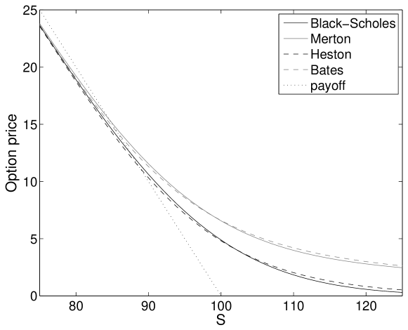
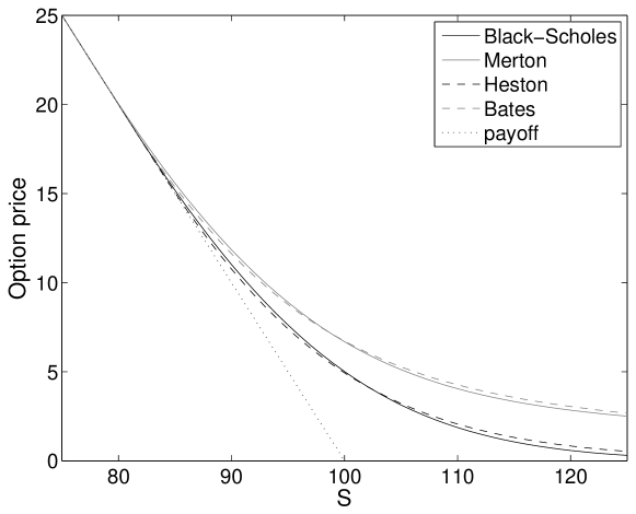
For the purpose of illustration, Fig. 1 and Fig. 2 show fair values of European and American options, respectively, under the four considered models with the model parameters described in the following sections.

Figure 1: The fair values of European put options for the asset prices $75\leq s\leq 125$ and the volatility $\sigma=0.2$ (the variance $v=0.04$) under the four considered models.

Figure 2: The fair values of American put options for the asset prices $75\leq s\leq 125$ and the volatility $\sigma=0.2$ (the variance $v=0.04$) under the four considered models.

7.1 Black–Scholes model

In the case of the Black–Scholes model, we price American put options. The volatility in the model (1) is taken as

$$\sigma=0.2$$

and the following boundary conditions are employed:

$$u(0,t)= K ~{}~{}{\rm for}~{}~{}~{}0<t\leq T,$$ (38)

$$u_{s}(S_{\max},t)= 0 ~{}~{}{\rm for}~{}~{}~{}0<t\leq T.$$ (39)

The Neumann boundary condition (39) introduces a modeling error as it is not exactly fulfilled by the actual option price function. If $S_{\max}$ is taken sufficiently large, however, this error will be small in the region of interest.

For the spatial discretization of the Black–Scholes PDE (2), we apply FD formulas on nonuniform grids such that a large fraction of the grid points lie in the region of interest, that is, in the neighborhood of $s=K$.

For the construction of the spatial grid we adopt Haentjens12 . Let integer $m_{1}\geq 1$, constant $c>0$, and $0<S_{\rm{left}}<K<S_{\rm{right}}<S_{\max}$ be given. Let equidistant points $\xi_{\min}=\xi_{0}<\xi_{1}<\ldots<\xi_{m_{1}}=\xi_{\max}$ be given with distance $\Delta\xi$ and

$$\xi_{\min} =\sinh^{-1}\left(\frac{-S_{\rm{left}}}{c}\right),$$

$$\xi_{\rm{int}} =\frac{S_{\rm{right}}-S_{\rm{left}}}{c},$$

$$\xi_{\max} =\xi_{\rm{int}}+\sinh^{-1}\left(\frac{S_{\max}-S_{\rm{right}}}{c}\right).$$

Then we define a nonuniform grid $0=s_{0}<s_{1}<\ldots<s_{m_{1}}=S_{\max}$ by the transformation

$$s_{i}=\varphi(\xi_{i})\quad(0\leq i\leq m_{1}),$$ (40)

where

$$\varphi(\xi)=\begin{cases}S_{\rm{left}}\,\,+c\cdot\sinh(\xi)&~{}(\xi_{\min}\leq\xi\leq 0),\\ S_{\rm{left}}\,\,+c\cdot\xi&~{}(0<\xi<\xi_{\rm{int}}),\\ S_{\rm{right}}+c\cdot\sinh(\xi-\xi_{\rm{int}})&~{}(\xi_{\rm{int}}\leq\xi\leq\xi_{\max}).\end{cases}$$

The grid (40) is uniform inside $[S_{\rm{left}},S_{\rm{right}}]$ and nonuniform outside. The parameter $c$ controls the fraction of grid points $s_{i}$ that lie inside $[S_{\rm{left}},S_{\rm{right}}]$. The grid is smooth in the sense that there exist real constants $C_{0},C_{1},C_{2}>0$ such that the grid sizes $\Delta s_{i}=s_{i}-s_{i-1}$ satisfy

$$C_{0}\,\Delta\xi\leq\Delta s_{i}\leq C_{1}\,\Delta\xi\quad{\rm and}\quad|\Delta s_{i+1}-\Delta s_{i}|\leq C_{2}\left(\Delta\xi\right)^{2}$$ (41)

uniformly in $i$ and $m_{1}$. For the parameters in the grid we make the (heuristic) choice

$$S_{\max}=8K,~{}~{}c=\frac{K}{10},~{}~{}S_{\rm{left}}=\max\left(\tfrac{1}{2},e^{-T/10}\right)K~{},~{}~{}S_{\rm{right}}=\min\left(\tfrac{3}{2},e^{T/10}\right)K.$$

The semidiscretization of the initial-boundary value problem for the Black–Scholes PDE is then performed as follows. At the interior grid points each spatial derivative appearing in (2) is replaced by its corresponding second-order central FD formula described in Section 4. At the boundary $s=S_{\max}$ the Neumann condition (39) gives $\partial u/\partial s$. Next, $\partial^{2}u/\partial s^{2}$ is approximated by the central formula with the value at the virtual point $S_{\max}+\Delta s_{m_{1}}$ defined by linear extrapolation using (39).

Concerning the initial condition, we always replace the value of the payoff function $\phi$ at the grid point $s_{i}$ nearest to the strike $K$ by its cell average,

$$\frac{1}{h}\int_{s_{i-1/2}}^{s_{i+1/2}}\max(K-s,0)\,ds,$$

where

$$s_{i-1/2}=\tfrac{1}{2}(s_{i-1}+s_{i}),~{}~{}s_{i+1/2}=\tfrac{1}{2}(s_{i}+s_{i+1}),~{}~{}h=s_{i+1/2}-s_{i-1/2}.$$

This reduces the dependency of the discretization error on the location of the strike relative to the $s$-grid, see e.g. Tavella00 .

The time discretization is performed by the Crank–Nicolson method with Rannacher smoothing. The time stepping is started by taking two backward Euler steps using the time step $\tfrac{1}{2}\Delta t$. With this choice all time steps are performed with the same coefficient matrix ${\bf I}-\tfrac{1}{2}\Delta t{\bf A}$. Furthermore, halving the time step with the Euler method helps to reduce the additional error caused by this method. Note that we count these two Euler steps as one time step in order to keep the notations convenient.

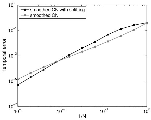
We define the temporal discretization error to be

$$\widehat{e}(m_{1},N)=\max\left\{\,|U_{N,i}-U_{i}(T)|:~{}\tfrac{1}{2}K<s_{i}<\tfrac{3}{2}K\right\},$$ (42)

where $U_{N,i}$ denotes the component of the vector $U_{N}$ associated to the grid point $s_{i}$. We study the temporal discretization errors on the grids $(m_{1},N)=(160,2^{k})$ for $k=0,1,\ldots,10$. The reference price vector $U(T)$ is computed using the space-time grid $(160,5000)$. Fig. 3 compares the temporal errors of the smoothed Crank–Nicolson method with and without the operator splitting method for LCPs described in Section 5.4. For larger time steps the Crank–Nicolson method without splitting is more accurate. In this example the convergence rate of the splitted method is slightly less than second-order and a bit higher than the convergence rate of the unsplitted method. Thus, for smaller time steps the operator splitting method is slightly more accurate.

Figure 3: The temporal discretization errors for the American option under the Black–Scholes model for the smoothed Crank–Nicolson method with and without the operator splitting method for LCPs.

7.2 Merton model

Under the Merton jump diffusion model, we price European and American put options. For the jump part of the model, the jump activity, the mean of the normal distribution, and its standard deviation are taken as

$$\lambda=0.2,~{}~{}\delta=0.4,~{}~{}\text{and}~{}~{}\gamma=-0.5,$$ (43)

respectively; see (8). The boundary condition at $s=0$ is given by (5) for the European put option and by (38) for the American put option. At the truncation boundary $s=S_{\max}$, we use the Neumann boundary condition (39).

The same space-time grids are considered as with the Black–Scholes model in Section 7.1 and also the spatial derivatives are discretized in the same way. For the integral term, we use a linear interpolation for $u$ between grid points and take $u$ to be zero for $s>S_{\max}$. The formulas for the resulting matrix ${\bf J}$ are given in Salmi11 , for example.

For the time discretization, we apply the IMEX–CNAB scheme, which is always smoothed by two Euler steps with the time step $\tfrac{1}{2}\Delta t$. In these first steps the backward Euler method is used for the discretized differential part ${\bf D}$ and the forward Euler method is used for the discretized integral part ${\bf J}$. For European options, these steps are given by

$$\begin{split}\left({\bf I}-\tfrac{\Delta t}{2}{\bf D}\right)U_{1/2}&=U_{0}+\tfrac{\Delta t}{2}{\bf J}U_{0}+\tfrac{\Delta t}{2}G_{1/2},\\ \left({\bf I}-\tfrac{\Delta t}{2}{\bf D}\right)U_{1}&=U_{1/2}+\tfrac{\Delta t}{2}{\bf J}U_{1/2}+\tfrac{\Delta t}{2}G_{1}.\end{split}$$

In the absence of jumps, these steps reduce to the same Rannacher smoothing used with the Black–Scholes model. After these two steps the IMEX–CNAB scheme defined by (26) is employed.

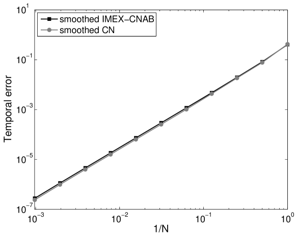
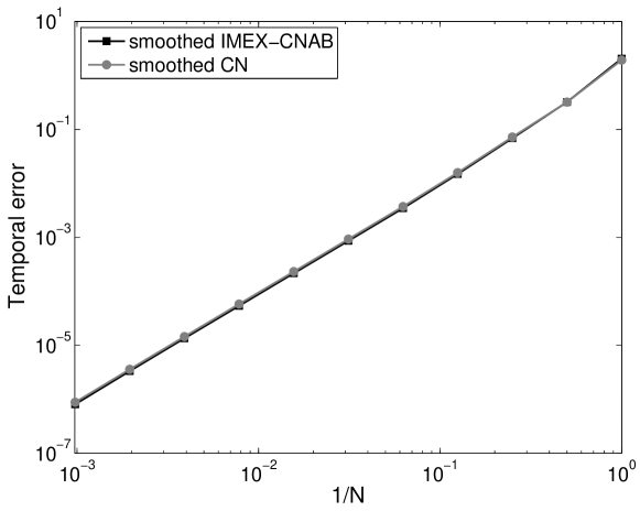
We study the temporal discretization errors for European and American options on the same grids $(m_{1},N)=(160,2^{k})$, $k=0,1,\ldots,10$, and using the same error measure (42) as before. Fig. 4 shows the temporal errors for the European option using the IMEX–CNAB scheme and the Crank–Nicolson method with classical Rannacher smoothing. We observe that the temporal errors for the two methods are essentially the same and they exhibit second-order convergence.

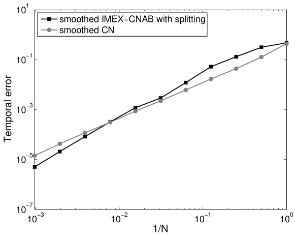
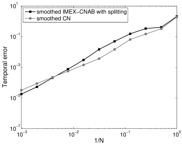
Fig. 6 shows the same temporal errors for American options using the IMEX–CNAB scheme with operator splitting for LCPs and the Crank–Nicolson method without splitting. The convergence result for the two methods is very similar to the case of the Black–Scholes model in Section 7.1. Thus, for larger time steps the Crank–Nicolson method is more accurate while for smaller time steps the IMEX–CNAB scheme with splitting is more accurate.

In order to gauge the effectiveness of the proposed discretizations, we report the total discretization errors for the European option on the space-time refining grids $(m_{1},N)=2^{k}(10,2)$, $k=0,1,\ldots,6$. The total discretization error is defined by

$$e(m_{1},N)=\max\left\{\,|U_{N,i}-u(s_{i},T)|:~{}\tfrac{1}{2}K<s_{i}<\tfrac{3}{2}K\right\}.$$ (44)

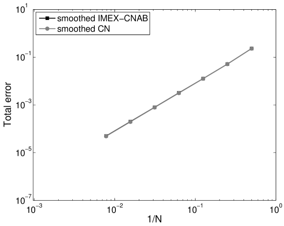
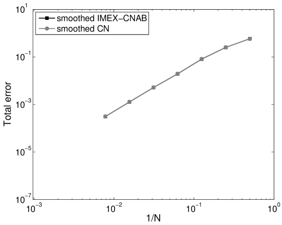
The reference price function $u$ is computed on the space-time grid $(10240,2048)$. Fig. 5 shows the total error for the European option using the IMEX–CNAB scheme and the Crank–Nicolson method. As with the temporal errors the total errors for both methods are essentially the same and both show a second-order convergence behavior.

Figure 4: The temporal discretization errors for the European option under the Merton model with the IMEX–CNAB scheme and the Crank–Nicolson method, both with smoothing.

Figure 5: The total discretization errors for the European option under the Merton model with the IMEX–CNAB scheme and the Crank–Nicolson method, both with smoothing.

Figure 6: The temporal discretization errors for the American option under the Merton model with the IMEX–CNAB scheme together with the operator splitting method for LCPs, and the Crank–Nicolson method, both with smoothing.

7.3 Heston model

Under the Heston stochastic volatility model we consider European and American put options as well. For the mean-reversion rate, the long-term mean, the volatility-of-variance and the correlation the following values are taken:

$$\kappa=2,~{}~{}\eta=0.04,~{}~{}\sigma=0.25,~{}~{}\text{and}~{}~{}\rho=-0.5.$$ (45)

The spatial domain is truncated to $[0,S_{\max}]\times[0,V_{\max}]$ with $S_{\max}=8K$ and $V_{\max}=5$. The following boundary conditions are imposed:

$$u(0,v,t)= d\!f\cdot K ~{}~{}{\rm for}~{}~{}~{}0\leq v\leq V_{\max},~{}0<t\leq T,$$ (46)

$$u_{s}(S_{\max},v,t)= 0 ~{}~{}{\rm for}~{}~{}~{}0\leq v\leq V_{\max},~{}0<t\leq T,$$ (47)

$$u_{v}(s,V_{\max},t)= 0 ~{}~{}{\rm for}~{}~{}~{}0\leq s\leq S_{\max},~{}0<t\leq T,$$ (48)

where $d\!f=e^{-rt}$ in the European case and $d\!f=1$ in the American case. At the degenerate boundary $v=0$ the Heston PDE holds in the European case and it is assumed that the Heston LCP holds in the American case. The two conditions at $s=S_{\max}$ and $v=V_{\max}$ introduce a modeling error, as they are not exactly fulfilled by the actual option price function, but in our experiments this error is small on the region of interest in the $(s,v)$-domain.

For the spatial discretization of the Heston PDE and Heston LCP we apply FD formulas on Cartesian grids. Here nonuniform grids are used in both the $s$- and $v$-directions such that a large fraction of the grid points lie in the neighborhoods of $s=K$ and $v=0$, respectively. This is the region in the $(s,v)$-domain where one wishes to obtain option prices. Next, the application of such nonuniform grids can greatly improve the accuracy of the FD discretization as compared to using uniform grids. This is related to the facts that the initial function (4) possesses a discontinuity in its first derivative at $s=K$ and that for $v\approx 0$ the Heston PDE is convection-dominated. The grid in the $s$-direction is taken identical to that in Section 7.1.

To construct the grid in the $v$-direction, let integer $m_{2}\geq 1$ and constant $d>0$ and let equidistant points be given by $\psi_{j}=j\cdot\Delta\psi$ for $j=0,1,\ldots,m_{2}$ with

$$\Delta\psi=\frac{1}{m_{2}}\,\sinh^{-1}\left(\frac{V_{\max}}{d}\right).$$

Then a smooth, nonuniform grid $0=v_{0}<v_{1}<\ldots<v_{m_{2}}=V_{\max}$ is defined by

$$v_{j}=d\cdot{\rm sinh}(\psi_{j})\quad(0\leq j\leq m_{2}).$$ (49)

The parameter $d$ controls the fraction of grid points $v_{j}$ that lie near $v=0$. We heuristically choose

$$d=\frac{V_{\max}}{500}\,.$$

The semidiscretization of the initial-boundary value problem for the Heston PDE and Heston LCP is performed as follows. In view of the Dirichlet condition (46), the grid in $[0,S_{\max}]\times[0,V_{\max}]$ is given by $\{(s_{i},v_{j}):1\leq i\leq m_{1},~{}0\leq j\leq m_{2}\}.$ At this grid, each spatial derivative is replaced by its corresponding second-order central FD formula described in Section 4 with a modification for the boundaries $v=0$, $s=S_{\max}$, and $v=V_{\max}$.

At the boundary $v=0$ the derivative $\partial u/\partial v$ is approximated using a second-order forward formula. All other derivative terms in the $v$-direction vanish at $v=0$, and therefore do not require further treatment.

At the boundary $s=S_{\max}$ the spatial derivatives in the $s$-direction are dealt with as in Section 7.1. Note that the Neumann condition (47) at $s=S_{\max}$ implies that the mixed derivative $\partial^{2}u/\partial s\partial v$ vanishes there.

At the boundary $v=V_{\max}$ the spatial derivatives in the $v$-direction need to be considered. This is done fully analogously to those in the $s$-direction at $s=S_{\max}$ using now the Neumann condition (48).

Define the temporal discretization error by

$$\widehat{e}(m_{1},m_{2},N)=\max\left\{\,|U_{N,l}-U_{l}(T)|:~{}\tfrac{1}{2}K<s_{i}<\tfrac{3}{2}K,~{}0<v_{j}<1\right\},$$ (50)

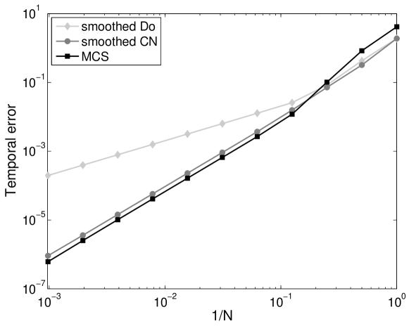
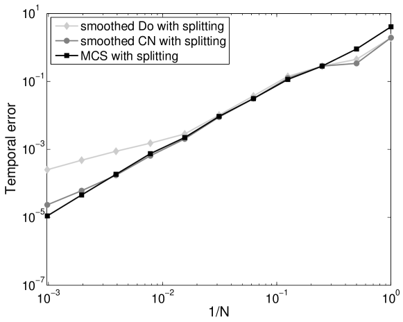
where the index $l$ corresponds to the grid point $(s_{i},v_{j})$. The reference vector $U(T)$ is computed using $(m_{1},m_{2},N)=(160,80,5000)$. We study these errors for $(m_{1},m_{2},N)=(160,80,2^{k})$ with $k=0,1,\ldots,10$ and three methods: the Do scheme with $\theta=\frac{1}{2}$ and smoothing, the MCS scheme with $\theta=\frac{1}{3}$ without smoothing, and the Crank–Nicolson scheme with smoothing.

Fig. 7 displays the obtained results for the European put option. As a first observation, for all three methods the temporal errors are bounded from above by a moderate value and decrease monotonically as $N$ increases. The error graphs for the MCS and Crank–Nicolson schemes are almost identical and reveal a second-order convergence behavior. The Do scheme only shows first-order convergence. Clearly, the convergence orders observed for the three methods agree with their respective classical orders of consistency. Additional experiments by substantially changing $(m_{1},m_{2})$ indicate that for all three methods the temporal errors are almost unaffected, which is a desirable property and suggests convergence in the so-called stiff sense. Whereas their results are not displayed, we mention that the CS scheme with $\theta=\frac{1}{2}$ and smoothing and the HV scheme with $\theta=\frac{1}{2}+\frac{1}{6}\sqrt{3}$ without smoothing behave similarly to the MCS scheme in this experiment, with slightly larger errors.

Fig. 9 displays the obtained results for the American put option. Our observations are analogous to those made above in the case of the European option. It is interesting to note, however, that the Do scheme often has temporal errors that are almost the same as for the MCS and Crank–Nicolson schemes. But if $N$ gets sufficiently large, then a first-order convergence behavior for this method indeed sets in. For the Crank–Nicolson scheme a small deviation from second-order is seen when $N$ is large. This disappears however when other values $(m_{1},m_{2})$ are considered. Additional experiments by substantially changing $(m_{1},m_{2})$ indicate that for all three methods the temporal errors are at most mildly affected.

We next consider, in the European put option case, the total discretization error defined by

$$e(m_{1},m_{2},N)=\max\left\{\,|U_{N,l}-u(s_{i},v_{j},T)|:~{}\tfrac{1}{2}K<s_{i}<\tfrac{3}{2}K,~{}0<v_{j}<1\right\},$$ (51)

with index $l$ corresponding to the grid point $(s_{i},v_{j})$. Here exact solution values $u$ are computed by a suitable implementation of Heston’s semi-closed form analytical formula Heston93 . Note that the modeling error, which is due to the truncation of the domain of the Heston PDE to a bounded set, is also contained in $e(m_{1},m_{2},N)$. In our experiment, this contribution is negligible.

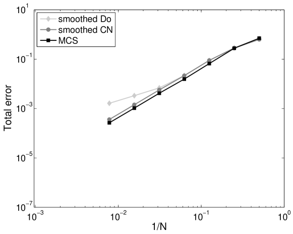
Fig. 8 displays the total discretization errors for $(m_{1},m_{2},N)=2^{k}(10,5,2)$ with $k=0,1,\ldots,6$ and the three schemes under consideration in this section. With the MCS and Crank–Nicolson schemes the total errors are essentially the same and a second-order convergence behavior is observed. With the Do scheme, the total errors are almost same as these two schemes up to $k=4$, but then the convergence drops to the expected first-order.

For a more extensive numerical study of ADI schemes in the (two-dimensional) Heston model we refer to intHout10 for European-style options and to Haentjens15 for American-style options. For three-dimensional PDEs in finance, such as the HHW PDE, the numerical convergence of ADI schemes has been investigated in Haentjens13a ; Haentjens12 and for a four-dimensional PDE in Haentjens13c . In these references a variety of parameter sets has been considered, including long maturity times and cases where the Feller condition is strongly violated, together with various barrier options and the approximation of hedging quantities.

Figure 7: Temporal discretization errors in the case of the European put option under the Heston model. The time discretization methods are: the Do scheme with $\theta=\frac{1}{2}$ and smoothing, the MCS scheme with $\theta=\frac{1}{3}$ without smoothing, and the Crank–Nicolson scheme with smoothing.

Figure 8: Total discretization errors in the case of the European put option under the Heston model. The time discretization methods are: the Do scheme with $\theta=\frac{1}{2}$ and smoothing, the MCS scheme with $\theta=\frac{1}{3}$ without smoothing, and the Crank–Nicolson scheme with smoothing.

Figure 9: Temporal discretization errors in the case of the American put option under the Heston model. The time discretization methods are: the Do scheme with $\theta=\frac{1}{2}$ and smoothing, the MCS scheme with $\theta=\frac{1}{3}$ without smoothing, and the Crank–Nicolson scheme with smoothing.

7.4 Bates model

We price European and American put options under the Bates model. The boundary conditions are given by (46)–(48). For the stochastic volatility part of the model the parameters are taken the same as for the Heston model and they are given by (45). For the jump part, the parameters are the same as for the Merton model and they are given by (43). The discretizations are based on the same grids and the spatial derivatives are discretized in the same way as with the Heston model in Section 7.3. For the jump integral, the same discretization is used as with the Merton model in Section 7.2. We consider here the IMEX–CNAB scheme and Crank–Nicolson method both applied with smoothing as for the Merton model.

As with the Heston model, we consider the temporal discretization errors on the grids $(m_{1},m_{2},N)=(160,80,2^{k})$, $k=0,1,\ldots,10$. The reference price vector $U(T)$ is computed using the space-time grid $(160,80,5000)$. The temporal discretization errors $\widehat{e}(m_{1},m_{2},N)$ are shown for the European option in Fig. 10 and for the American option in Fig. 12. The plots show the errors for the IMEX–CNAB scheme and the Crank–Nicolson method. For the American option the operator splitting method for LCPs is used with the IMEX–CNAB scheme. As with other models, the temporal errors for the European option are very similar for both methods and they both exhibit second-order convergence. For the American option, the difference between the methods is less pronounced than with the Black–Scholes and Merton models. Still the Crank–Nicolson method is slightly more accurate than the operator splitting method for large time steps and the reverse is true for small time steps. In this example the convergence rates seem to be between 1.5 and 2.0.

We computed the total discretization errors $e(m_{1},m_{2},N)$ for the European option on the grids $(m_{1},m_{2},N)=2^{k}(10,5,2)$, $k=0,1,\ldots,6$. The reference prices are computed on the space-time grid $(2560,1280,512)$. Fig. 11 shows the total errors for the IMEX–CNAB scheme and the Crank–Nicolson method. As with the other models, the total errors for both methods are virtually the same and both have second-order convergence of the total error.

Figure 10: The temporal discretization errors for the European option under the Bates model with the IMEX–CNAB scheme and the Crank–Nicolson method, both with smoothing.

Figure 11: The total discretization errors for the European option under the Bates model with the IMEX–CNAB scheme and the Crank–Nicolson method, both with smoothing.

Figure 12: The temporal discretization errors for the American option under the Bates model with the IMEX–CNAB scheme together with the operator splitting method for LCPs, and the Crank–Nicolson method, both with smoothing.

8 Conclusions

We have discussed numerical solution methods for financial option valuation problems in the contemporary partial(-integro) differential equations framework. These problems are often multidimensional and can involve nonlocal integral operators due to jumps incorporated in the underlying asset price models. The early exercise feature of American-style options gives rise to linear complementarity problems, which are nonlinear. All these properties add complexity to the discrete problems obtained by classical implicit numerical methods and renders their efficient solution a challenging task. The efficient computation of option values is, however, crucial in many applications. In this chapter an overview has been given of various types of operator splitting methods for the discretization in time, which yield in each time step a sequence of discrete subproblems that can be handled much more easily and efficiently without essentially influencing the accuracy of the underlying discretization. The following highlights the different operator splitting methods presented in this chapter.

For multidimensional models the directional splitting methods of the ADI type offer a fast, accurate, and easy-to-implement way for the numerical time stepping. They are adapted to effectively deal with mixed spatial derivative terms, which are ubiquitous in finance. ADI schemes lead to a sequence of sparse linear subproblems that can be solved by LU decomposition at optimal computational cost, that is, the number of required operations is directly proportional to the number of unknowns. The MCS and HV schemes, with a proper choice of their parameter $\theta$, are recommended as these show stability and second-order convergence and reveal a better inherent smoothing than second-order CS.

The spatial discretization of jumps models for the underlying asset price yields dense matrices. All classical implicit time discretization schemes require solving systems with these dense matrices. By employing an IMEX method like the IMEX–CNAB scheme advocate here, with an explicit treatment of (finite activity) jumps and an implicit treatment of the remainder of the operator, each time step involves only multiplications with these dense matrices. This is computationally a much easier task and can be often performed very fast using FFT. The accuracy and stability of the IMEX–CNAB scheme are good when the jump activity is not very high, e.g. less than several jumps per year.

Iterative methods like the PSOR method for solving LCPs resulting from the pricing of American-style options often converge slowly. We discussed an operator splitting method based on a Lagrange multiplier formulation, treating in each time step the early exercise constraint and complementarity condition in separate subproblems, where the main subproblem is essentially the same as for the European-style counterpart. With this approach it is easy to adapt a European option pricer to American options. We presented such an adaptation for ADI and IMEX methods. Also, it is applicable for most models of underlying asset prices. Numerical experience with this operator splitting method indicates that the accuracy stays essentially the same as in the case of the original LCP, but there can be a major reduction in computational time.

References

- (1) Achdou, Y., Pironneau, O.: Computational methods for option pricing, Frontiers in Applied Mathematics, vol. 30. Society for Industrial and Applied Mathematics (SIAM), Philadelphia, PA (2005)
- (2) Almendral, A., Oosterlee, C.W.: Numerical valuation of options with jumps in the underlying. Appl. Numer. Math. 53(1), 1–18 (2005)
- (3) Andersen, L., Andreasen, J.: Jump-diffusion processes: Volatility smile fitting and numerical methods for option pricing. Rev. Deriv. Res. 4(3), 231–262 (2000)
- (4) Andersen, L.B.G., Piterbarg, V.V.: Interest rate modeling, volume I: foundations and vanilla models. Atlantic Financial Press (2010)
- (5) Bank for International Settlements: Triennial Central Bank Survey, Foreign exchange turnover in April 2013: preliminary global results (2013)
- (6) Bates, D.S.: Jumps and stochastic volatility: Exchange rate processes implicit in Deutsche Mark options. Review Financial Stud. 9(1), 69–107 (1996)
- (7) Black, F., Scholes, M.: The pricing of options and corporate liabilities. J. Political Economy 81, 637–654 (1973)
- (8) Brandt, A., Cryer, C.W.: Multigrid algorithms for the solution of linear complementarity problems arising from free boundary problems. SIAM J. Sci. Statist. Comput. 4(4), 655–684 (1983)
- (9) Brennan, M.J., Schwartz, E.S.: The valuation of American put options. J. Finance 32, 449–462 (1977)
- (10) Briani, M., Natalini, R., Russo, G.: Implicit-explicit numerical schemes for jump-diffusion processes. Calcolo 44(1), 33–57 (2007)
- (11) Carr, P., Geman, H., Madan, D.B., Yor, M.: The fine structure of asset returns: an empirical investigation. J. Business 75, 305–332 (2002)
- (12) Carr, P., Mayo, A.: On the numerical evaluation of option prices in jump diffusion processes. Eur. J. Finance 13, 353–372 (2007)
- (13) Chorin, A.J.: Numerical solution of the Navier-Stokes equations. Math. Comp. 22, 745–762 (1968)
- (14) Clark, I.J.: Foreign exchange option pricing. Wiley, Chichester (2011)
- (15) Clarke, N., Parrott, K.: Multigrid for American option pricing with stochastic volatility. Appl. Math. Finance 6, 177–195 (1999)
- (16) Cont, R., Tankov, P.: Financial modelling with jump processes. Chapman & Hall/CRC, Boca Raton, FL (2004)
- (17) Cont, R., Voltchkova, E.: A finite difference scheme for option pricing in jump diffusion and exponential Lévy models. SIAM J. Numer. Anal. 43(4), 1596–1626 (2005)
- (18) Craig, I.J.D., Sneyd, A.D.: An alternating-direction implicit scheme for parabolic equations with mixed derivatives. Comput. Math. Appl. 16, 341–350 (1988)
- (19) Cryer, C.W.: The solution of a quadratic programming problem using systematic overrelaxation. SIAM J. Control 9, 385–392 (1971)
- (20) Dang, D.M., Christara, C.C., Jackson, K.R., Lakhany, A.: A PDE pricing framework for cross-currency interest rate derivatives. Proc. Comp. Sc. 1, 2371–2380 (2010)
- (21) Davis, T.A.: Direct methods for sparse linear systems, Fundamentals of Algorithms, vol. 2. Society for Industrial and Applied Mathematics (SIAM), Philadelphia, PA (2006)
- (22) d’Halluin, Y., Forsyth, P.A., Vetzal, K.R.: Robust numerical methods for contingent claims under jump diffusion processes. IMA J. Numer. Anal. 25(1), 87–112 (2005)
- (23) Douglas, J., Rachford, H.H.: On the numerical solution of heat conduction problems in two and three space variables. Trans. Amer. Math. Soc. 82, 421–439 (1956)
- (24) Egloff, D.: GPUs in financial computing part III: ADI solvers on GPUs with application to stochastic volatility. Wilmott Magazine (March), 51–53 (2011)
- (25) Ekström, E., Tysk, J.: The Black–Scholes equation in stochastic volatility models. J. Math. Anal. Appl. 368, 498 –507 (2010)
- (26) Feng, L., Linetsky, V.: Pricing options in jump-diffusion models: an extrapolation approach. Oper. Res. 56(2), 304–325 (2008)
- (27) Forsyth, P.A., Vetzal, K.R.: Quadratic convergence for valuing American options using a penalty method. SIAM J. Sci. Comput. 23(6), 2095–2122 (2002)
- (28) Frank, J., Hundsdorfer, W., Verwer, J.G.: On the stability of implicit-explicit linear multistep methods. Appl. Numer. Math. 25(2-3), 193–205 (1997)
- (29) George, A.: Nested dissection of a regular finite element mesh. SIAM J. Numer. Anal. 10, 345–363 (1973). Collection of articles dedicated to the memory of George E. Forsythe
- (30) Glowinski, R.: Numerical methods for nonlinear variational problems. Scientific Computation. Springer-Verlag, New York (1984)
- (31) Glowinski, R.: Splitting methods for the numerical solution of the incompressible Navier-Stokes equations. In: Vistas in applied mathematics, Transl. Ser. Math. Engrg., pp. 57–95. Optimization Software, New York (1986)
- (32) Grzelak, L.A., Oosterlee, C.W.: On the Heston model with stochastic interest rates. SIAM J. Financial Math. 2(1), 255–286 (2011)
- (33) Grzelak, L.A., Oosterlee, C.W., Van Weeren, S.: Extension of stochastic volatility equity models with the Hull-White interest rate process. Quant. Finance 12(1), 89–105 (2012)
- (34) Haentjens, T.: ADI schemes for the efficient and stable numerical pricing of financial options via multidimensional partial differential equations. PhD thesis. University of Antwerp (2013)
- (35) Haentjens, T.: Efficient and stable numerical solution of the Heston–Cox–Ingersoll–Ross partial differential equation by alternating direction implicit finite difference schemes. Int. J. Comput. Math. 90(11), 2409–2430 (2013)
- (36) Haentjens, T., in ’t Hout, K.J.: Alternating direction implicit finite difference schemes for the Heston–Hull–White partial differential equation. J. Comput. Finance 16(1), 83–110 (2012)
- (37) Haentjens, T., in ’t Hout, K.J.: ADI schemes for pricing American options under the Heston model. Appl. Math. Finance (2015). URL http://dx.doi.org/10.1080/1350486X.2015.1009129
- (38) Heston, S.L.: A closed-form solution for options with stochastic volatility with applications to bond and currency options. Review Financial Stud. 6, 327–343 (1993)
- (39) in ’t Hout, K.J., Foulon, S.: ADI finite difference schemes for option pricing in the Heston model with correlation. Int. J. Numer. Anal. Model. 7(2), 303–320 (2010)
- (40) in ’t Hout, K.J., Mishra, C.: Stability of the modified Craig–Sneyd scheme for two-dimensional convection-diffusion equations with mixed derivative term. Math. Comput. Simulation 81(11), 2540–2548 (2011)
- (41) in ’t Hout, K.J., Mishra, C.: Stability of ADI schemes for multidimensional diffusion equations with mixed derivative terms. Appl. Numer. Math. 74, 83–94 (2013)
- (42) in ’t Hout, K.J., Welfert, B.D.: Stability of ADI schemes applied to convection-diffusion equations with mixed derivative terms. Appl. Numer. Math. 57(1), 19–35 (2007)
- (43) in ’t Hout, K.J., Welfert, B.D.: Unconditional stability of second-order ADI schemes applied to multi-dimensional diffusion equations with mixed derivative terms. Appl. Numer. Math. 59(3-4), 677–692 (2009)
- (44) Huang, J., Pang, J.S.: Option pricing and linear complementarity. J. Comput. Finance 2, 31–60 (1998)
- (45) Hull, J.C.: Options, futures and other derivatives. Pearson Education, Harlow (2011)
- (46) Hull, J.C., White, A.: Pricing interest-rate-derivative securities. Review Financial Stud. 3, 573–592 (1990)
- (47) Hundsdorfer, W.: Accuracy and stability of splitting with Stabilizing Corrections. Appl. Numer. Math. 42, 213–233 (2002)
- (48) Hundsdorfer, W., Verwer, J.G.: Numerical solution of time-dependent advection-diffusion-reaction equations, Computational Mathematics, vol. 33. Springer, Berlin (2003)
- (49) Ikonen, S., Toivanen, J.: Operator splitting methods for American option pricing. Appl. Math. Lett. 17(7), 809–814 (2004)
- (50) Ikonen, S., Toivanen, J.: Componentwise splitting methods for pricing American options under stochastic volatility. Int. J. Theor. Appl. Finance 10(2), 331–361 (2007)
- (51) Ikonen, S., Toivanen, J.: Pricing American options using LU decomposition. Appl. Math. Sci. (Ruse) 1(49-52), 2529–2551 (2007)
- (52) Ikonen, S., Toivanen, J.: Efficient numerical methods for pricing American options under stochastic volatility. Numer. Methods Partial Differential Equations 24(1), 104–126 (2008)
- (53) Ikonen, S., Toivanen, J.: Operator splitting methods for pricing American options under stochastic volatility. Numer. Math. 113(2), 299–324 (2009)
- (54) Itkin, A., Carr, P.: Jumps without tears: a new splitting technology for barrier options. Int. J. Numer. Anal. Model. 8(4), 667–704 (2011)
- (55) Jaillet, P., Lamberton, D., Lapeyre, B.: Variational inequalities and the pricing of American options. Acta Appl. Math. 21(3), 263–289 (1990)
- (56) Kou, S.G.: A jump-diffusion model for option pricing. Management Sci. 48(8), 1086–1101 (2002)
- (57) Kwon, Y., Lee, Y.: A second-order finite difference method for option pricing under jump-diffusion models. SIAM J. Numer. Anal. 49(6), 2598–2617 (2011)
- (58) Kwon, Y., Lee, Y.: A second-order tridiagonal method for American options under jump-diffusion models. SIAM J. Sci. Comput. 33(4), 1860–1872 (2011)
- (59) Lipton, A.: Mathematical methods for foreign exchange. World Scientific, Singapore (2001)
- (60) Marchuk, G.I.: Splitting and alternating direction methods. Handb. Numer. Anal., I. North-Holland, Amsterdam (1990)
- (61) McKee, S., Mitchell, A.R.: Alternating direction methods for parabolic equations in two space dimensions with a mixed derivative. Computer J. 13, 81–86 (1970)
- (62) McKee, S., Wall, D.P., Wilson, S.K.: An alternating direction implicit scheme for parabolic equations with mixed derivative and convective terms. J. Comput. Phys. 126, 64–76 (1996)
- (63) Merton, R.C.: Theory of rational option pricing. Bell J. Econom. Management Sci. 4, 141–183 (1973)
- (64) Merton, R.C.: Option pricing when underlying stock returns are discontinuous. J. Financial Econ. 3, 125–144 (1976)
- (65) Oosterlee, C.W.: On multigrid for linear complementarity problems with application to American-style options. Electron. Trans. Numer. Anal. 15, 165–185 (2003)
- (66) Peaceman, D.W., Rachford, H.H.: The numerical solution of parabolic and elliptic differential equations. J. Soc. Ind. Appl. Math. 3, 28–41 (1955)
- (67) Rannacher, R.: Finite element solution of diffusion problems with irregular data. Numer. Math. 43(2), 309–327 (1984)
- (68) Reisinger, C., Wittum, G.: On multigrid for anisotropic equations and variational inequalities: pricing multi-dimensional European and American options. Comput. Vis. Sci. 7(3-4), 189–197 (2004)
- (69) Ruge, J.W., Stüben, K.: Algebraic multigrid. In: Multigrid methods, Frontiers Appl. Math., vol. 3, pp. 73–130. SIAM, Philadelphia, PA (1987)
- (70) Saad, Y., Schultz, M.H.: GMRES: a generalized minimal residual algorithm for solving nonsymmetric linear systems. SIAM J. Sci. Statist. Comput. 7(3), 856–869 (1986)
- (71) Salmi, S., Toivanen, J.: An iterative method for pricing American options under jump-diffusion models. Appl. Numer. Math. 61(7), 821–831 (2011)
- (72) Salmi, S., Toivanen, J.: Comparison and survey of finite difference methods for pricing American options under finite activity jump-diffusion models. Int. J. Comput. Math. 89(9), 1112–1134 (2012)
- (73) Salmi, S., Toivanen, J.: IMEX schemes for pricing options under jump-diffusion models. Appl. Numer. Math. 84, 33–45 (2014)
- (74) Seydel, R.U.: Tools for computational finance. Springer, London (2012)
- (75) Shreve, S.E.: Stochastic calculus for finance II. Springer, New York (2008)
- (76) Stüben, K.: Algebraic multigrid: An introduction with applications. In: Multigrid. Academic Press Inc., San Diego, CA (2001)
- (77) Tavella, D., Randall, C.: Pricing financial instruments: The finite difference method. John Wiley & Sons (2000)
- (78) Toivanen, J.: Numerical valuation of European and American options under Kou’s jump-diffusion model. SIAM J. Sci. Comput. 30(4), 1949–1970 (2008)
- (79) Toivanen, J.: A componentwise splitting method for pricing American options under the Bates model. In: Applied and numerical partial differential equations, Comput. Methods Appl. Sci., vol. 15, pp. 213–227. Springer, New York (2010)
- (80) Toivanen, J.: Finite difference methods for early exercise options. In: R. Cont (ed.) Encyclopedia of Quantitative Finance. John Wiley & Sons (2010)
- (81) Toivanen, J., Oosterlee, C.W.: A projected algebraic multigrid method for linear complementarity problems. Numer. Math. Theory Methods Appl. 5(1), 85–98 (2012)
- (82) Trottenberg, U., Oosterlee, C.W., Schüller, A.: Multigrid. Academic Press Inc., San Diego, CA (2001). With contributions by A. Brandt, P. Oswald and K. Stüben
- (83) Verwer, J.G., Spee, E.J., Blom, J.G., Hundsdorfer, W.: A second-order Rosenbrock method applied to photochemical dispersion problems. SIAM J. Sci. Comput. 20, 1456–1480 (1999)
- (84) van der Vorst, H.A.: Bi-CGSTAB: A fast and smoothly converging variant of Bi-CG for the solution of nonsymmetric linear systems. SIAM J. Sci. Stat. Comp. 13, 631–644 (1992)
- (85) Wilmott, P.: Derivatives. John Wiley & Sons Ltd., Chichester (1998)