Records in the classical and quantum standard map

Abstract

Record statistics is the study of how new highs or lows are created and sustained in any dynamical process. The study of the highest or lowest records constitute the study of extreme values. This paper represents an exploration of record statistics for certain aspects of the classical and quantum standard map. For instance the momentum square or energy records is shown to behave like that of records in random walks when the classical standard map is in a regime of hard chaos. However different power laws is observed for the mixed phase space regimes. The presence of accelerator modes are well-known to create anomalous diffusion and we notice here that the record statistics is very sensitive to their presence. We also discuss records in random vectors and use it to analyze the quantum standard map via records in their eigenfunction intensities, reviewing some recent results along the way.

1 Introduction

Breaking a record, or setting a new one has been a human passion, perhaps one may say weakness, for a while now. Evidence how one yearns for a record to be set by a particular sportsperson or the euphoria (depression) that sets in when the stock market fluctuations reach a maximum (minimum) never seen before. Of course our view of nature also abounds in such characterizations: the highest mountains, the deepest oceans, the smallest temperatures reached and so on. While these may seem to be questions about extremes, records are a record of extremes, the times they last and the number of new ones created. For engineers designing a dam, one important piece of information is when and by how much the water level of the river has exceeded all its previous values; similar questions are naturally asked about rainfall when planning for agricultural policies is taken up. Practical considerations such as these have been the early applications in a study of events which exceed themselves in some aspect and are often called as “record statistics”, akin to the study of extreme statistics in many ways. An accessible introduction to record statistics is found in Schmittmann and Zia (1999).

Questions about how the records increase with time, or the number of records set, are of natural interest in all these complex, sometimes social contexts, have therefore been studied for example, Gembris et al. (2002); Vogel et al. (2001); Redner and Petersen (2006). A mathematical theory of records for independent identically distributed (i.i.d.) random variables has been developed since the pioneering work of Rényi (1962) for example developed in Glick (1978); Arnold et al. (1998). The applications in Physics started somewhat later, but have by now found use in various problems related to random walks, spin-glasses, type II superconductors and quantum chaos. In this work, our emphasis is on the record statistics in deterministic dynamical systems, both classical and quantum. In particular we choose the most studied low-dimensional paradigm of Hamiltonian chaos, namely the standard map, or known variously as the kicked-rotor, Chirikov-Taylor map etc.. Its quantization has also been extensively studied, as well as realized experimentally in cold atom set ups in Moore et al. (1995).

Now to define records more precisely, given that $\{X_{t},t=1,\cdots,N\}$ is a finite time series, the first element, $R(1)$, of the corresponding records series is $X_{1}$ itself and at subsequent times $t$ it will be $R(t)=\mbox{max}(X_{t},R(t-1))$. As $X_{t}$ is a random variable, so is $R(t)$ and properties of this random variable is of interest. Thus $R(t)$ which consists of elements of $X_{t}$ in a non-decreasing order are the upper record sequence. If the minimum value is taken instead of the maximum the record sequence is called the lower record sequence. From the definition of records, it is clear that last upper (lower) record is also the global maximum (minimum) of the sequence $\{X_{j}\}$. Hence, the statistics of last record will correspond to similar results of maximum or minimum from extreme value theory. A word of caution is warranted here, as the second last upper (lower) record will not be the second maximum (minimum) of the sequence. This can be easily understood by visualizing a sequence $X_{t}$ whose global maximum (minimum) occurs before second maximum (minimum). As in that case, record statistics will not sense the presence of second maximum (minimum). To develop more familiarity with record sequence, let’s take $\sin x,~{}0\leq x\leq 2\pi$ as an example. In the range $[0,\pi/2]$ the upper record sequence is $\sin x$ itself and beyond that the entries will be constant 1.

Our motivations in this study are many. Firstly, while there is an elegant and simple theory of records for the case of independent random variables, we can naturally expect interesting departures for correlated processes. One such class of problems, namely random walks, have been studied in this context and remarkable departures and universalities have been uncovered. One of our motivations is to see how much of this survives for deterministic dynamical systems. For instance it has been appreciated now for more than 40 years that deterministic systems such as the kicked rotor can display normal diffusion, as well as anomalous diffusion. It is then of interest to ask if the record statistics behaves in the same manner as that of random walks in this scenario, and what happens in the different diffusion regimes. Also related question is how do the record statistics change as the system undergoes a transition to chaos. The latter question is natural here, but not so in the setting of random walks. We also wish to go on to explore quantum dynamics and review some of our recent works on record statistics. In this publication, all the material pertaining to record statistics in the classical standard map or kicked rotor is new, so also detailed derivations of the record statistics for delta correlated variables, as well the lower record statistics. Some other material, having to do with eigenfunction statistics have been partially presented in publications before (see Srivastava et al. (2013)) and is included here as a brief review.

1.1 Independent and identically distributed (i.i.d.) random variables

Consider the entries of $\{X_{j}\}$ as being independent and identically distributed random numbers. As we have exchangeable entries, the symmetry of the sequence determines the probability of $X_{j}$ being a record to be $1/j$ at the $j^{th}$ trial; see Rényi (1962) or Arnold et al. (1998). In other words, any of the $j$ entries till $X_{j}$, including itself, is equally possible to be the record. Consider temperatures in a particular city, despite all the fluctuations, it is clear that it beats its own record. In formal language, the process of setting a record is persistent. Let us denote the number of records in a sequence of length $n$ by $N_{n}$, then the above statement can be rephrased as $N_{n}\rightarrow\infty$ with length of sequence $n\rightarrow\infty$.

The next natural question is about the frequency with which records are broken. Define an indicator function

$$I_{j}=\left\{\begin{array}[]{ll}1&\textrm{if there is a record at $j$ },\\ 0&\textrm{otherwise}.\end{array}\right.$$ (1)

Calculating the expected value of $I_{j}$ is equivalent to calculating the probability of $I_{j}$ taking the value 1, but this is precisely the probability of $X_{j}$ being the record- which is $1/j$. Thus $\langle I_{j}\rangle=1/j$. Similarly, for variance, we note that expected value of $I_{j}^{2}$ is the same as expected value of $I_{j}$. This immediately gives the variance as $1/j-1/j^{2}$. It can be easily proven that $I_{j}$ are pairwise uncorrelated (statistically independent). In other words the probability of the position of the records is a Bernoulli process, $\mbox{Ber}(1/j)$.

As the total number of records $N_{n}$ in a sequence $\{X_{1},X_{2},\cdots X_{n}\}$ is $\sum_{j=1}^{n}I_{j}$, the expectation and variance can be readily calculated:

$$\langle N_{n}\rangle =\sum_{j=1}^{n}\langle I_{j}\rangle=\sum_{j=1}^{n}\frac{1}{j}=H_{n}.$$ (2)

$$V(N_{n}) =\sum_{j=1}^{n}V(I_{j})=\sum_{j=1}^{n}\frac{1}{j}-\sum_{j=1}^{n}\frac{1}{j^{2}}.$$

Here $H_{n}$ is the $n^{th}$ harmonic number. A remarkable, well-known fact from the theory of records is that for i.i.d. variables these quantities are distribution-free, that is independent of the particular underlying distribution $p(x)$, see Arnold et al. (1998). For example the average number of records $\langle N_{n}\rangle=H_{n}\sim\log(n)+\gamma$, where $\gamma$ is the Euler constant, is indeed very small compared to the length $n$ of the data set; typically records are rare events in independent processes. From the above it immediately follows that the variance also grows as $\log(n)$. Next section on, we will change the notation from $N_{n}$ to $N_{R}$.

1.2 Random walks and records

Some of the recent works concerns the behavior of records in correlated processes, for example see Majumdar and Ziff (2008); Wergen et al. (2011); Schehr and Majumdar (2013). One important class of such processes are random walks and the few studies on their record statistics is now very briefly reviewed. In case of random walks, $x_{t}$ represents the position of a random walker at a time step, $t$. For discrete time steps and jump-lengths drawn from an i.i.d. symmetric distribution, Majumdar and Ziff showed that the probability $P(M,N)$ of $M$ records in $t=N$ steps is given by

$$P(M,N)=\binom{2N-M+1}{N}2^{-2N+M-1},\quad M\leq N+1$$ (3)

with mean $\langle M\rangle\sim\frac{2}{\sqrt{\pi}}\sqrt{N}$. Age statistics of record i.e., how long a record survives before it is broken, is given by $\langle l\rangle\sim\frac{N}{\langle M\rangle}\sim\sqrt{\frac{\pi N}{4}}$ (Majumdar and Ziff (2008)). Thus in strong contrast to the i.i.d. case, the number of records is very large.

This makes physical sense, as the random walker is indeed trying to go somewhere and each time she has genuinely progressed in a particular direction a record is set. Being diffusive, this process is certainly slower than ballistic, and in fact grows in the same way as the distance from the origin. That said, it is then interesting and somewhat surprising that it retains the property of being universal in that it is independent of the exact distribution of the jump-lengths. In fact even when distributions have a fat tail (like Cauchy distribution), this result has been shown to be valid by Majumdar and Ziff (2008).

In the case of continuous time random walks, i.e. when position of a random walker is now observed at equal discrete time steps with time interval $\tau_{0}$, the probability $P(M,t)$ of finding $M$ records within a given time duration $t$, as derived by Sabhapandit (2011), and attains a scaling form given by,

$$P(M,t) \sim(t/\tau_{0})^{-\alpha/2}g_{\alpha}\left(M(t/\tau_{0})^{-\alpha/2}\right)$$ (4)

$$g_{\alpha}(x) =\frac{2}{\alpha}x^{-(1+2/\alpha)}L_{\alpha/2}(x^{-2/\alpha}),\quad 0<\alpha\leq 1,$$

where $L_{\alpha/2}(x)$ is a one-sided Lévy stable probability distribution function. The moments of records, asymptotically go as

$$\langle M^{\nu}\rangle\sim\frac{(2/\alpha)\Gamma(\nu)}{\Gamma(\nu\alpha/2)}(t/\tau_{0})^{\nu\alpha/2}.$$ (5)

The mean-age of the record is

$$\langle l\rangle=\langle t/M\rangle\sim\frac{\tau_{0}(\alpha/2)}{\Gamma(1-\alpha/2)}[\ln(t/\tau_{0})-\Psi(1-\alpha/2)](t/\tau_{0})^{(1-\alpha)},$$ (6)

where $\Psi(x)$ is di-gamma function, see Sabhapandit (2011). The parameter $\alpha\in(0,1)$, appearing as exponent of power law decay of the waiting time distribution decides the qualitative behavior of record statistics.

In another generalization due to Wergen et al. (2011), the record distribution for a random walk with discrete time steps but asymmetric jump distribution, has been calculated for the model governed by $x_{n}=x_{n-1}+\xi_{n}+c$ with $\xi_{n}$ being the jump length with symmetric distribution while $c$ is the constant drift. For Gaussian jump distribution with variance $\sigma$, in the limit of small drift (smallness is compared with respect to $c=0$ case) i.e. $\left(\frac{c}{\sigma}\ll\frac{1}{\sqrt{n}}\right)$, the mean number of records and record rate (i.e. probability of $n^{th}$ event being a record), is given by,

$$\langle M_{n}(c)\rangle \approx\frac{2\sqrt{n}}{\sqrt{\pi}}+\frac{c}{\sigma}\frac{\sqrt{2}}{\pi}(n\arctan(\sqrt{n})-\sqrt{n}),$$ (7)

$$P_{n}(c) \approx\frac{1}{\sqrt{\pi n}}\frac{c}{\sigma}\frac{\sqrt{2}}{\pi}\arctan(\sqrt{n}).$$

In the large drift limit, $P_{n}(c)$ approaches a constant value Wergen et al. (2011). Later, this problem was exactly solved for arbitrary value of constant bias $c$ and a number of interesting results have been obtained such as the qualitatively different regions in the space of $c,\mu$ by Majumdar et al. (2012) where $\mu$ is the Lévy index for symmetric stable law of jump distribution.

1.3 Application of record statistics in superconductors and quantum chaos

The geometric feature of random systems such as size of the largest cluster in percolation on a finite lattice of size $N$, has been shown to follow Gumbel distribution in the large-$N$ limit by Bazant (2000). In type-II superconductors, temperature independence of the magnetic creep rate i.e. rate of change of magnetic field in the sample at a constant temperature for a range of temperatures has been understood in terms of record dynamics, namely, the dynamical properties of the times at which a stochastic fluctuating signal (in this case thermal noise due to non-zero temperature) establishes records. This puzzling temperature independence of the creep rate, which at non-zero temperatures has its origin due to thermal fluctuations, has been sorted out by showing that the process of vortex penetration into the sample can be described in terms of a Poisson process with logarithmic time argument, called the log-Poisson process; a result from record dynamics by Oliveira et al. (2005).

The application of record statistics in case of quantum chaos has been treated in Srivastava et al. (2013). It is known that the eigenstate intensities in fully chaotic systems with no particular symmetries are conjectured to behave exactly as these random vectors subject only to a normalization constraint. These are also the statistical properties of eigenvectors of the classical ensembles of random matrix theory. For chaotic systems, the applicability of random matrix theory Mehta (2004); Brody et al. (1981) has been well appreciated for long Bohigas et al. (1984). As we will discuss in detail in Section 3 for the standard map the breaking of the last KAM torus allows for diffusion in phase space and diffusion being connected with random walks, we expect and indeed observe the average number of records in eigenvectors to go as $\sqrt{N}$. In fact this is first known instance where $K$ values at which the last KAM torus breaks has been seen in a quantity derived from quantum mechanical spectrum.

2 Records in $\delta$-correlated variables

2.1 Upper records for complex random vectors

For a correlated sequence, let the probability density for a record variable $R$, at time $t$ be $P(R,t)$. The average record is given by $\left\langle R\right\rangle=\int\mathop{\mathrm{\mathstrut d}}\nolimits\!R~{}RP(R,t)$. Let $P(x_{1},\ldots,x_{N})$ be the j.p.d.f. of $N$ random variables. The probability that the record at time $t$, is less than $R$ is given by (for example Srivastava et al. (2013)):

$$Q(R,t)=\int_{0}^{R}\mathop{\mathrm{\mathstrut d}}\nolimits\!x_{1}\cdots\mathop{\mathrm{\mathstrut d}}\nolimits\!x_{t}P_{t}(x_{1},...x_{t})$$ (8)

where $P_{t}(x_{1},\ldots,x_{t})=\int P(x_{1},\ldots,x_{N})\mathop{\mathrm{\mathstrut d}}\nolimits\!x_{t+1}\cdots\mathop{\mathrm{\mathstrut d}}\nolimits\!x_{N}$ is the marginal j.p.d.f. of the first $t$ random variables . It follows that $P(R,t)=\mathop{\mathrm{\mathstrut d}}\nolimits\!Q(R,t)/\mathop{\mathrm{\mathstrut d}}\nolimits\!R$.

Let us specialize to the case of $\delta$ correlated random variables i.e. sum of the random entries is a constant. For example, components of normalized complex random vectors $z_{n}=\langle n|\psi\rangle$, have the j.p.d.f:

$$P(z_{1},z_{2},\ldots,z_{N})=(\Gamma(N)/\pi^{N})\delta\left(\sum_{j=1}^{N}|z_{j}|^{2}-1\right).$$ (9)

This is also the distribution of the components of the eigenvectors of the GUE or CUE (Gaussian or Circular unitary ensembles) random matrices, for example see the book by Haake (1991). It is the invariant uniform distribution under an arbitrary unitary transformations on the $2N-1$ dimensional sphere. It is the unique (Haar) measure on $S^{2N-1}$. The normalization provides correlation among the components that becomes weak for large $N$. The intensities $x_{i}=|z_{i}|^{2}$ being the random variables of interest it is more useful to define the j.p.d.f. directly in terms of these:

$$P(x_{1},\dots,x_{N};u)=\Gamma(N)\delta\left(\sum_{i=1}^{N}x_{i}-u\right),$$ (10)

where $u$ is an auxiliary quantity, the actual j.p.d.f. corresponding to $u=1$.

The delta constraint also arises in problems such as the “broken-stick” one, wherein a stick is broken into a fixed number of pieces but with random lengths. The delta correlation is a very weak constraint, and in fact it is not hard to conclude on some reflection that the number of records and its statistics remains unaffected by this correlation. The way in which a set of random numbers can be correlated by the delta function, gives us a hint: take i.i.d random normal variables and normalize them, then the resulting set of numbers are uniformly distributed on some sphere and hence are delta correlated. But the rank order remains the same on a normalization process and hence the record statistics remains the same. Note that we have here the new variables $x_{i}$ being distributed uniformly on a simplex rather than a sphere: however this does not matter for the records as again the act of taking a square does not affect the rank order. Nevertheless we show this explicitly here, as we derive the probability of the value of the record itself, which does differ from the uncorrelated case. Also our analysis generalizes in a significant way an earlier analysis of extreme values in such random variables by Lakshminarayan et al. (2008).

Defining

$$Q(R,t;u)=\int_{0}^{R}\mathop{\mathrm{\mathstrut d}}\nolimits\!x_{1}\cdots\mathop{\mathrm{\mathstrut d}}\nolimits\!x_{t}\int_{0}^{\infty}P(x_{1},\dots,x_{N};u)\mathop{\mathrm{\mathstrut d}}\nolimits\!x_{t+1}\cdots\mathop{\mathrm{\mathstrut d}}\nolimits\!x_{N}$$ (11)

leads to

$$\int_{0}^{\infty}e^{-su}Q(R,t;u)\mathop{\mathrm{\mathstrut d}}\nolimits\!u=\frac{\Gamma(N)}{s^{N}}\sum_{m=0}^{t}(-1)^{m}\binom{t}{m}e^{-smR}.$$ (12)

Using the convolution theorem, and then setting $u=1$ in $Q(R,t;u)$ gives

$$Q(R,t)=\sum_{m=0}^{t}(-1)^{m}\binom{t}{m}(1-mR)^{N-1}\Theta(1-mR).$$ (13)

Hence

$$P(R,t)=\sum_{m=1}^{t}(-1)^{m+1}\binom{t}{m}m(N-1)(1-mR)^{N-2}\Theta(1-mR),$$ (14)

the probability density that the record is $R$ at time $t$. Note that $P(R,N)$ is the probability density that the maximum value of the entire data set is $R$, which was calculated for the case of random GUE vectors in Lakshminarayan et al. (2008) and therefore $P(R,t)$ here is a generalization. The piecewise smooth probability distribution found there has a similar behavior here.

It was shown in Lakshminarayan et al. (2008) that $P(R,N)$ is Gumbel distributed asymptotically. In fact the generalization presented in Eq. (13) is also Gumbel distributed for large $N$, as for large $N$ and large $t\gg 1$

$$Q(R,t)\approx(1-\exp(-NR))^{t}\approx\exp\left(-t\exp(-NR)\right).$$ (15)

Since the Gumbel distribution is of the form $\exp[-\exp(-(x-a_{N})/b_{N}]$ where $a_{N}$ and $b_{N}$ are the shift and scaling. It follows that for the record statistics the relevant parameters are $a_{N}=\log(t)/N$ and $b_{N}=1/N$. The shift generalizes from $\log(N)/N$ for the maximum, while the scaling remains the same. The above form also appears in the limit when the correlations are ignored.

The average value of the record as a function of time is

$$\langle R(t)\rangle=1-\int_{0}^{1}Q(R,t)\,dR=\frac{1}{N}\sum_{m=1}^{t}(-1)^{m+1}\frac{1}{m}\binom{t}{m}=\frac{H_{t}}{N}=\frac{1}{N}\sum_{k=1}^{t}\frac{1}{k},$$ (16)

where $H_{t}$ is a Harmonic number as defined above. Known asymptotics of the Harmonic numbers implies that

$$\langle R(t)\rangle=\frac{1}{N}\left(\gamma+\ln(t)+\frac{1}{2t}-\sum_{k=1}^{\infty}\frac{B_{2k}}{2k\,t^{2k}}\right),$$ (17)

where $B_{2k}$ are Bernoulli numbers, and $\gamma$ is the Euler-Mascheroni constant. Again, this presents a generalization of the average maximum intensity found in Lakshminarayan et al. (2008) which corresponds to $t=N$.

It is not hard to prove that for intensities of random states too, the probability of the position of the records is a Bernoulli process although they are correlated by the normalization constraint. Let there be records at positions $(j_{1}=1<j_{2}<\cdots<j_{m})$ and let $I_{J_{k}}=1$ if there is a record at $j_{k}$ or $0$ otherwise. Then the j.p.d.f.

$$\mbox{Prob}(I_{j_{1}}=1,I_{j_{2}}=1,\ldots,I_{j_{m}}=1)=\int_{{\cal C}}P(x_{1},\ldots,x_{N};u=1)dx_{1}\cdots dx_{N}=\prod_{k=1}^{m}\frac{1}{j_{k}}.$$ (18)

Here ${\cal C}$ is the set of constraints: $0\leq x_{k}\leq x_{j_{2}},$ $j_{1}\leq k\leq j_{2}-1$; $0\leq x_{k}\leq x_{j_{3}},$ $j_{2}\leq k\leq j_{3}-1$; $\cdots$, $0\leq x_{k}\leq x_{j_{m}},$ $j_{m-1}\leq k\leq j_{m}-1$; $0\leq x_{k}\leq 1$, $j_{m}\leq k\leq N$. The above result follows on using the Laplace transform to free the constraint in Eq. (10). However this is the result for i.i.d. random variables, and implies that the occurrence of a record at $j_{k}$ is an independent process, as the above is valid for all arbitrary choices of the locations $j_{k}$. Hence $\mbox{Prob}(I_{j}=1)=1/j$ and $\mbox{Prob}(I_{j}=0)=1-1/j$, in other words the process is $\mbox{Ber}(1/j)$.

The average number of records is thus

$$\langle N_{R}\rangle=\left\langle\sum_{j=1}^{N}I_{j}\right\rangle=\sum_{j=1}^{N}\frac{1}{j}=H_{N},$$ (19)

while as a random variable $N_{R}$ has a distribution essentially given by the signless Stirling numbers of the first kind, some times called the Karamata-Stirling law (see Nevzorov (1987)). Such laws hold for a variety of disparate processes including the number of cycles in a random permutation of $N$ objects, number of nodes in extreme side branch of random binary search trees etc. Bai et al. (1998). Being distribution-free, the number of records is a statistics that directly detects correlations.

The probability that the final record, which is the maximum in the entire data sequence, lasts for time $m$ can also be simply calculated: denoted $S_{N}(m)=P(I_{N}=0,I_{N-1}=0,\cdots,I_{N-m+2}=0,I_{N-m+1}=1)=1/N$, it is (somewhat surprisingly) independent of $m$, and uniform. This implies that the position at which the maximum occurs is uniformly distributed. The implications of this for quantum chaotic wavefunctions where strong scarring effects of classical periodic orbits ( see McDonald and Kaufman (1979); Heller (1984); Biswas and Jain (1990); Kudrolli et al. (1995); Laurent et al. (2007)) can affect the maxima of states is of natural interest, and will be discussed below.

2.2 Lower records in complex random vectors

The question of a record minimum can be asked in a similar way, the cumulative density function for a record minimum, i.e. the probability that the record is “greater” than $R$ at a time $t$ is given by

$$Q(R,t)=\int_{R}^{\infty}\mathop{\mathrm{\mathstrut d}}\nolimits\!x_{1}\cdots\mathop{\mathrm{\mathstrut d}}\nolimits\!x_{t}P_{t}(x_{1},\dots,x_{t})$$ (20)

where $P(x_{1},\dots,x_{N})$ is j.p.d.f. of $N$ random variables, and $P_{t}(x_{1},\dots,x_{t})$ is the j.p.d.f. of $t$ random variables given by $\int_{all~{}range}P(x_{1},\dots,x_{N})\mathop{\mathrm{\mathstrut d}}\nolimits\!x_{t+1}\dots\mathop{\mathrm{\mathstrut d}}\nolimits\!x_{N}$. From $Q(R,t)$ we can get $P(R,t)$ as

$$P(R,t)=-\frac{\mathop{\mathrm{\mathstrut d}}\nolimits\!Q(R,t)}{\mathop{\mathrm{\mathstrut d}}\nolimits\!R}.$$ (21)

It is not difficult to calculate the probability distribution of record minima in the case of a complex random vector, essentially following the same technique as in the case of maximum records,

$$Q(R,t;s) = \Gamma(N)e^{-s\sum_{i=1}^{t}r_{i}}\left[\prod_{i=1}^{t}\int_{R}^{\infty}\mathop{\mathrm{\mathstrut d}}\nolimits\!r_{i}e^{-sr_{i}}\right]\left[\prod_{i=t+1}^{N}\int_{0}^{\infty}\mathop{\mathrm{\mathstrut d}}\nolimits\!r_{i}e^{-sr_{i}}\right]$$

$$= \frac{\Gamma(N)}{s^{N-t}}\frac{e^{-sRt}}{s^{t}}$$

Using the convolution theorem and then replacing $u=1$, we get

$$Q(R,t)=(1-Rt)^{N-1}\Theta(1-Rt)$$ (22)

Density,

$$P(R,t)=-\frac{dQ(R,t)}{dR}=(N-1)t(1-Rt)^{N-2}\Theta(1-Rt)$$ (23)

and average record as a function of $t$ can be easily found

$$\langle R(t)\rangle = \int RP(R,t)\mathop{\mathrm{\mathstrut d}}\nolimits\!R$$

$$= \frac{1}{Nt}.$$

Again this generalizes the results obtained in Lakshminarayan et al. (2008). For large $N$ limit $Q(R,t)$ is again exponential and for $t=N$, it retrieves all the results obtained in Lakshminarayan et al. (2008). In particular while the average intensity is $1/N$,the average minimum intensity is $1/N^{2}$ corresponding to $t=N$. The record low intensity is inversely proportion to the “time”, which in the case of static wavefunctions is the index of the basis used. It is easy to show (by just changing the conditions and hence the limits in appropriate integrations) that these are also Bernoulli process, $\mbox{Ber}\left(1/n\right)$ and hence all the results for survival probability, lifetime distribution etc. remains same in this case too. We remark that the exponential form of $Q(R,t)$ in the large $N$ limit is a special case of the Weibull distribution of the standard theory of extreme value statistics of i.i.d. random variables.

3 Record statistics in the classical and quantum standard map

Attention is now turned to the standard map. This is chosen as the standard map is a simply defined dynamical system which has a well-studied transition to chaos through the usual route of smooth two-degree of freedom Hamiltonian systems. It also has a simple and well-studied quantization and allows breaking parity and time-reversal symmetries through quantum phases and hence allows for studying GUE, GOE, (or CUE, COE), as well as intermediate statistics. Before discussing the record statistics for eigenvectors we summarize some aspects of the standard map pertaining to quantization and the intensity distribution of its eigenvectors.

3.1 Elementary aspects of the standard map

We recall for convenience some well-known basic aspects of the standard map. The Hamiltonian of the $\delta$-kicked rotor is given by

$$H(q,p,t)=\frac{p^{2}}{2}-\frac{g}{4\pi^{2}}\cos(2\pi q)\sum_{n=-\infty}^{\infty}\delta\left(t/T-n\right).$$ (24)

On rescaling $Tp\rightarrow p$ and $T^{2}g\rightarrow K$, this results in the area-preserving map:

$$q_{n+1} = (q_{n}+p_{n})~{}\mbox{mod}~{}1,$$

$$p_{n+1} = p_{n}-\frac{K}{2\pi}\sin(2\pi q_{n+1}),$$ (25)

connecting the position and momentum just after kick $n$ ($q_{n},p_{n})$ to that after kick $n+1$. This is the Chirikov-Taylor map or standard map. The fixed points $(0,0)$, $(1/2,0)$ of this map are stable and unstable respectively for small $K$.

The periodic property of $q$ endows the phase space with the topology of a cylinder. It is also well known that the translational boost in momentum by $n\in\mathbb{Z}$ is a symmetry of the standard map, and this allows one to take the modulo 1 for momentum as well and hence endows the topology of the two-torus to the phase space. Similarly, it also enjoys a discrete symmetry of reflection about the centre of square i.e. $p\rightarrow(1-p)$, $q\rightarrow(1-q)$. In the limit $K=0$, this map is completely integrable and with the increase in $K$, destruction and creation of invariant surface (i.e. KAM tori) takes place.

About $K\approx 1$, the last rotationally invariant KAM torus breaks, allowing global diffusion in the momentum space. If the standard map is unfolded to a cylinder it displays normal diffusion in momentum for large enough $K$. When $K\gg 5$, the classical map is essentially fully chaotic. While for very small $K$ the phase space seems to constitute only invariant curves, the $K=10$ case appears to be completely hyperbolic with no traces of islands. At $K\approx 1$ a well-known transition takes place when the last rotational KAM torus breaks and allows for global momentum transport when viewed on a cylindrical phase space. When $K<5$ the phase space is clearly mixed with large stable islands and chaotic regions coexisting.

To study the signatures of chaos in quantum mechanical spectrum of such systems has been the concern of the subject of “quantum chaos” or “quantum chaology”. Naturally quantization of such maps were the first step Casati and Ford (1979); Berry et al. (1979). Analogous to Eq. (3.1), Heisenberg equations can be integrated to yield similar equation for the operators. The unitary operator connecting states separated by a period of the kick is the quantum map. For the standard map on the plane, it is easy to see that corresponding unitary operator will be (Chang and Shi (1986); Izrailev (1999)),

$$\hat{U}=\exp\left(-\frac{igT}{2\pi^{2}\hbar}\cos(2\pi\hat{q})\right)\exp\left(-\frac{iT}{2\hbar}\hat{p}^{2}\right).$$ (26)

Due to periodicity in momentum and cyclic nature of the position variable, the natural phase space will be $[0,1)\times[0,1)$ so this map needs to be quantized on torus. The periodicity of both the canonical variables implies that the Hilbert space of quantum mechanics is finite dimensional. This dimensionality $N$ is related to a scaled Planck constant as $N=1/h$ and hence the classical limit is the large $N$ limit. A description can be found in the notes of Lakshminarayan (2009); Bäcker (2003).

The quantized standard map in position basis on torus takes the form,

$$U_{nn^{\prime}} = \frac{1}{N}\sum_{m=0}^{N-1}\exp\left[-i\pi\frac{(m+\beta)^{2}}{N}+2\pi i\frac{(m+\beta)}{N}(n-n^{\prime})\right]$$ (27)

$$\quad\quad\quad\quad\times\exp\left[i\frac{KN}{2\pi}\cos\frac{2\pi(n^{\prime}+\alpha)}{N}\right].$$

$\beta$ and $\alpha$ are the phases which a state acquires along position and momentum directions respectively. For periodic boundary conditions, $\beta=0$ while for anti-periodic, $\beta=1/2$. For all other $\beta$ values, time-reversal symmetry is broken. A similar role is played by $\alpha$ for parity symmetry. We will focus for the case, $\beta\neq 0$ and $\alpha\neq 0,1/2$ when we can expect that both the time-reversal symmetry and parity symmetry are broken and the typical eigenstates would be like complex random states.

To develop more familiarity with the intensities in different eigenfunctions of the quantum standard map, we have plotted them in Fig. 1 for $K=0.3,0.7$ and 5. It is clear that up to $K=1$, intensities are (almost) symmetric about $p=1/2$ despite $\alpha$ being $0.25$. This will have an impact when different aspects of record statistics of intensity vectors are considered.

\begin{overpic}[width=144.54pt]{husimi0p3st3} \par\put(18.0,60.0){\includegraphics[width=108.405pt]{k0p3_intensity3state}} \end{overpic}

(a)

\begin{overpic}[width=144.54pt]{husimi0p3st241} \put(18.0,50.0){\includegraphics[width=108.405pt]{k0p3_intensity241}} \end{overpic}

(b)

\begin{overpic}[width=144.54pt]{husimi0p7st33} \put(18.0,60.0){\includegraphics[width=108.405pt]{k0p7_intensity33}} \end{overpic}

(c)

\begin{overpic}[width=144.54pt]{husimi0p7st315} \put(18.0,50.0){\includegraphics[width=108.405pt]{k0p7_intensity315}} \end{overpic}

(d)

\begin{overpic}[width=144.54pt]{husimi5p0st7} \put(18.0,60.0){\includegraphics[width=108.405pt]{k5_intensity7}} \end{overpic}

(e)

\begin{overpic}[width=144.54pt]{husimi5p0st398} \put(18.0,60.0){\includegraphics[width=108.405pt]{k5_intensity398}} \end{overpic}

(f)

Figure 1: For different $K$ value the Husimi function, $|\langle q,p|\psi\rangle|^{2}$, of representative states and respective intensity plots are shown where $|q,p\rangle$ is coherent state which has been calculated following reference Saraceno (1990). Parity seems to be hold good for lower $K$ values despite the value of $\alpha$ being 0.25 (i.e. maximally broken parity).

3.2 Records and anomalous transport in the classical standard map

The transport of momentum in the standard map has been studied extensively. It is known that in the strongly chaotic regimes the diffusion might be normal or anomalous depending on the absence or presence of very special orbits, namely the accelerator modes. Thus momentum diffuses either as normal Brownian motion or if anomalous then as Lévy walks (Chirikov (1979); MacKay et al. (1984)). Recently a detailed analysis on the role of accelerator modes for anomalous diffusion has been carried out using the so-called GALI (Generalized ALignment Index) method (Manos and Robnik (2014)). In this section, numerical results for various quantities in the record statistics for momentum transport in the standard map is presented. The time series being studied are the squared deviation of momentum at $n^{\text{th}}$ iteration from the initial momentum. As have been already mentioned in the introduction that it has been shown in Majumdar and Ziff (2008), the average record for random walk or Levy walk (both), goes as $\sim\sqrt{4t/\pi}$ with time, $t$ while the variance of record depends on time linearly i.e. as $2(1-2/\pi)t$. It is then of interest to ask if this is the case for the standard map as well.

For large $K$, when the standard map is strongly chaotic, the distribution of position is uniform in range $[0,1)$. This suggests that in chaotic regime one can take the position variable as uncorrelated. Then, the standard map reduces to an effective one dimensional stochastic map:

$$p_{n+1}=p_{n}-\frac{K}{2\pi}\sin(2\pi r_{n})~{}~{}\text{with}~{}~{}r_{n}\in\text{Uniform}[0,1)$$ (28)

This is precisely the random walk with jump distribution taken from a i.i.d. distribution. This clearly brings out not only why the results for random walk can be expected to describe the results for record statistics for standard map in the hard chaos regime but also that any departure from it is due to correlations present in the steps of the deterministic dynamical system. For mixed phase regime, when a portion of phase space remains quasi-integrable, the time evolution of average records is expected to be sub-diffusive. But, any deviation in the large $K$ region can be a signature of accelerator modes.

Rewriting the Eq. 3.1 as

$$(p_{n}-p_{0})^{2}=\frac{K^{2}}{4\pi^{2}}\left(\sum_{i=0}^{n-1}\sin^{2}(2\pi q_{i})+\sum_{i\neq j}\sin(2\pi q_{i})\sin(2\pi q_{j})\right).$$ (29)

The record and the number of records for the quantity $(p_{n}-p_{0})^{2}$, namely the deviation in momentum square, are studied in this paper. Since, the square root of deviation in momentum square, as argued previously, will behave like random walk, the exponent in average record as a function of time will become 1 for true random walk cases. We have plotted the average record as a function of time in Fig. 2 and clearly the long-time behavior is a powerlaw $\propto t^{\alpha}$. The averaging is done over 10000 trajectories with initial conditions chosen uniformly from $[0,1)\times[0,1)$. The left panel corresponds to the case of mixed phase space or small $K$. We see the exponent increasing from values smaller than $1$ to $1$ and for $K=4.05$ be as high as $1.33$. At this value of $K$ there is still a mixed phase space regime, with the stable periodic orbit at $(0,0)$ having just undergone a bifurcation and having become unstable. This large value of the exponent may then arise from the presence of period-2 accelerator modes that have not nearly been studied as much as the usual period-1 modes.

Figure 2: Average record of deviation in momentum square as a function of time has been plotted on log-log scale. Clearly the long-time behaviour is $\propto t^{\alpha}$. (Left panel) $K$ values and the fitted exponent in the power law, are $K=0.5$, with $\alpha=0.11$ denoted by $\circ$, $K=2.00$, with $\alpha=0.86$ denoted by ${\color[rgb]{1,0,0}\Box}$, $K=3.2$ with $\alpha=1.009$ denoted by ${\color[rgb]{0,1,0}\Diamond}$ and $K=4.05,{\color[rgb]{0,0,1}\triangle}$ with $\alpha=1.33$. It is known that $K=4.05$, there exist an accelerator mode of period 2. (Right panel) The exponent $\alpha$ goes to $\sim 1$ for $K=10$ (denoted by ${\color[rgb]{1,0,0}\Box}$) i.e. in fully chaotic region. A slightly higher value of $\alpha$ for all the $K$ corresponding to the regime where accelerator modes are present in the phase space ($K=6.4$ with $\alpha=1.61$ denoted by $\circ$, $K=12.70,{\color[rgb]{0,1,0}\Diamond}$ with $\alpha=1.495$, $K=19.0,{\color[rgb]{0,0,1}\triangle}$ with $\alpha=1.3788$ and $K=25.25,{\color[rgb]{1,0,1}\ast}$ with $\alpha=1.2992$). The dashed lines are the fitting curves.

Figure 3: Average number of records as function of time has been shown for various $K$ values. The averaging is done over 10000 trajectories with initial conditions for position drawn uniformly from [0,1) and momentum from uniform distribution in $[0,1)$. (Left panel) $K$ values and the fitted exponent in the power law, are $K=0.5$, with $\alpha=0.22$ denoted by $\circ$, $K=2.00$, with $\alpha=0.47$ denoted by ${\color[rgb]{1,0,0}\Box}$, $K=3.2$ with $\alpha=0.51$ denoted by ${\color[rgb]{0,1,0}\Diamond}$ and $K=4.05,{\color[rgb]{0,0,1}\triangle}$ with $\alpha=0.53$. (Right panel) For hard chaos regime ($K=10$ denoted by ${\color[rgb]{1,0,0}\Box}$ with exponent 0.52) again the $\langle R_{n}\rangle$ varies in agreement with the analytical results for random walk. In figure, the various K values with the fitted straight lines are, $K=6.4$ with exponent 0.60, denoted by $\circ$, $K=12.70,{\color[rgb]{0,1,0}\Diamond}$ with exponent 0.57, $K=19.0,{\color[rgb]{0,0,1}\triangle}$ with exponent 0.55 and $K=25.25,{\color[rgb]{1,0,1}\ast}$ with exponent 0.54. The dashed lines are the fitting curves.The values quoted here are the best fitted exponents.

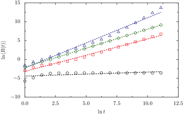
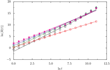
The right panel shows the case for $K\gg 5$ or hard chaos regime. At $K=10$ there is no evidence of any stable region or accelerator modes (Tomsovic and Lakshminarayan (2007)) and it is found that $\alpha\sim 1.0$. However the same figure also shows several other large $K$ values that deviates from this and has larger exponents. In all these values there are known accelerator modes. As we have averaged over 10000 trajectories with initial momentum drawn from uniform distribution in $[0,1)$, a few will satisfy the initial condition for accelerator modes which explains why the $\langle R(t)\rangle$ for $(p_{n}-p_{0})^{2}$ is not increasing quadratically with time. This shows that simple record statistics can be used as a signature to find the anomalous transport region. This clearly captures the presence of accelerator modes even of higher periods as can be seen in left panel of Fig. 2.

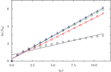
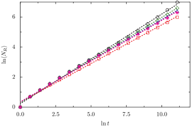
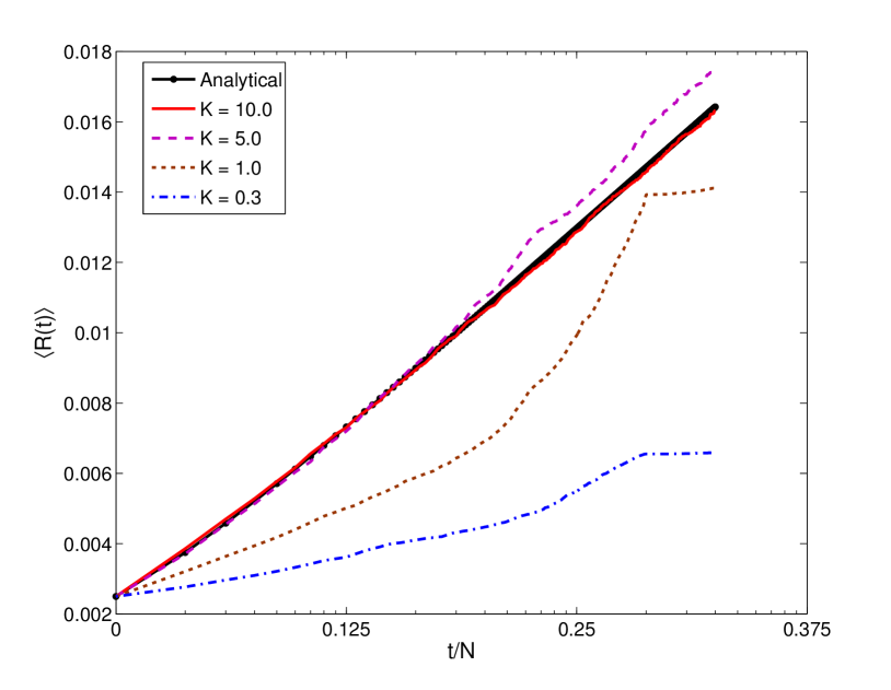
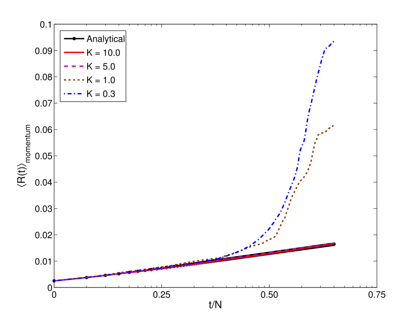
In Fig. 3, we have plotted the average number of records upto time $t$. Again the averaging is done over the ensemble of 10000 trajectories with initial conditions chosen uniformly from $[0,1)\times[0,1)$. The left panel again corresponds to a mixed phase space regime, while the right to hard chaos. Once again the same trends are observed and accelerator modes seem to have a strong influence on the number of records set. While in the absence of these special structures and for the case of hard chaos $N_{R}(t)\sim\sqrt{t}$, which is in agreement with the analytical results obtained in Majumdar and Ziff (2008) for random walks. This implies that the average time for which records lasts in the classical standard map’s diffusive regime also increases as $\sqrt{t}$ as in the random walk. It will be interesting to study the maximum and minimum intervals over which records last, but we have not pursued that here. In the case of random walks this has recently been studied by Godrèche et al. (2014).

However it should be pointed out that even if the steps lengths were that of a Levy walk the scaling was $\sqrt{t}$ for random walks, while in the case of a deterministic dynamical system, the Lévy walk leads to easily discernible departures. Thus these Lévy walks are evidently correlated ones and the correlation plays an important role here. Analytical studies of such walks is warranted in this context.

3.3 Record statistics for standard map eigenvector intensities

Let us briefly recall the intensity distribution expected from random matrix theory for a complex random state. As the expected value of each intensity component $x$ in an $N$ dimensional space is $1/N$, it will be convenient to transform to normalized variable $y=Nx$, and in the limit $N\rightarrow\infty$ its distribution becomes the exponential distribution,

$$\rho(y)=e^{-y}.$$ (30)

For $N=2048,~{}2050,~{}4096,~{}4098$, this is shown in Fig. 4. Except the tail region, it matches very well with the exponential distribution.

Figure 4: Intensity distribution for eigenvectors of standard map at $K=10$, $\alpha=0.25$, $\beta=0.25$ for different $N=2048,~{}2050,~{}4096,~{}4098$.

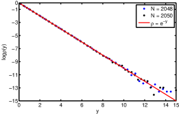
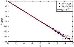
It is interesting to study the tail region, and the distribution of large intensities. Is there a pattern in observing larger intensities (“records”) as we go along the index of eigenvectors? What is the probability of occurrence of maximum intensity in, say the middle of the eigenfunction? These are some questions that we will be addressing comparing with the results obtained for random states in Section 2. For large $K$ quantum eigenstates of standard map follow the CUE/GUE or COE/GOE results depending on the value of the phases $\alpha$ and $\beta$. If $\beta\neq 0$ and $\alpha\neq 0,1/2$ we can expect that both the time-reversal symmetry and parity symmetry is broken and the typical eigenstates are expected to be like complex random states.

The wavefunctions are basis dependent and record statistics will in general depend on the space in which the eigenfunctions are represented. For small values of $K$ we expect there to be many localized states in the momentum space while being nearly uniformly distributed in the position, as the dominant invariant classical phase space structures are rotational KAM tori. However for large $K$, position or momentum basis will be equivalent statistically. Our analysis below is based on the quantum standard map on the torus. It is well known that the eigenstates of the quantum standard map on the cylinder are exponentially localized in momentum space (Izrailev (1999)) and share phenomenology similar to Anderson localization. Study of extremes or records in this case may also be interesting, but is not pursued further.

(a) position representation

(b) momentum representation

Figure 5: The average upper record $\langle R(t)\rangle$, from the ensemble of eigenstates of the quantum standard map. The parameters used are $N=400$ and $K=10$ (highly chaotic), $K=5$ (mostly chaotic), $K=1$ (mixed phase space), and $K=0.3$ (mostly regular). The analytical curve refers to the random state result in Eq. (17). In all cases $\alpha=\beta=0.25$.

The average value of the upper record as a function of the index for various values of $K$ is plotted in Fig. 5(a). This agrees well with the random states result in the chaotic region for example when $K=10$. However there are significant deviations in the mixed phase space regime. For example when $K=0.3$, in the position space most of the records are set up by $t/N=0.5$. It has been pointed out in Srivastava et al. (2013) that this feature is due to the weakly broken parity symmetry. There are significant deviations from the random state even for $K=5$ when the phase space is largely chaotic. The momentum space average records in the mixed phase space regime lie above the random state result and are not affected so much by the weakly broken parity symmetry due to their localization (see Fig. 5(b)). Thus for small $K$ we see much larger records being set than for the position space.

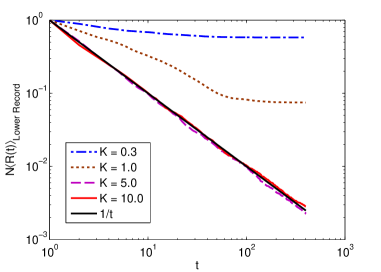
A similar picture appears with lower records as well, the results of random vector is followed for large $K(=10)$, while for smaller $K$ the records themselves do not vary with $t$ as compared to chaotic cases (see Fig. 6). As is clear that upper record and lower record combined will give the variation of the values that function assumes, let’s call it range, therefore in the case of standard map for smaller $K$ values (close to integrable regime), say $K=0.3$, average range of the intensities of eigenvectors is very small as compared to large $K$ values (chaotic regime), say $K=10$ (See Fig. 5(a) and Fig. 6). This is consistent with semiclassical analysis that for smaller value of $K$ invariant rotation KAM tori are not broken and therefore support wavefunctions with smaller range.

Figure 6: The average lower record $\langle R(t)\rangle_{\text{lower record}}$, from the ensemble of eigenstates of the quantum standard map in position representation. The parameters used are $N=400$ and $K=10$ (highly chaotic), $K=5$ (mostly chaotic), $K=1$ (mixed phase space), and $K=0.3$ (mostly regular). The analytical curve refers to the random state result in Eq. (2.2). In all cases $\alpha=\beta=0.25$.

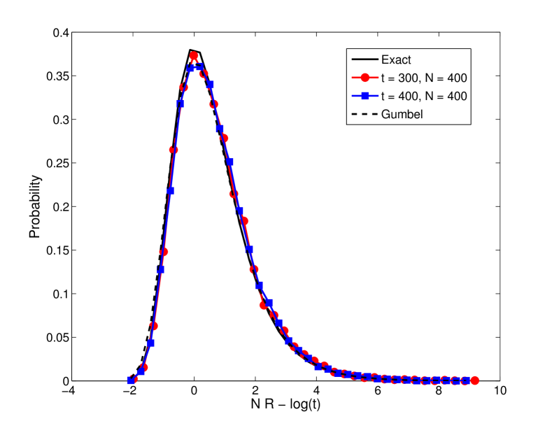
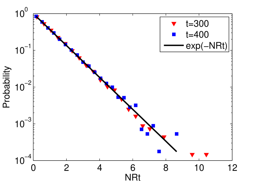
As has been previously discussed, the distribution of the upper (lower) record at “time” $t$ is Gumbel (exponential) for large $N$ with appropriate shift and scaling. It is shown in Fig. 7(a) (Fig. 7(b)) that indeed the upper (lower) record for eigenfunctions of the quantum standard map in the classically chaotic regime is Gumbel (exponentially)-distributed; also plotted is the distribution for the “upper (lower) record” when $t=N$ which refers to the maximum (minimum) intensity, thus recovering the earlier results of Lakshminarayan et al. (2008).

(a) upper record

(b) lower record

Figure 7: The distribution of the upper (lower) records when the index is $t$ for eigenfunctions of the quantum standard map with $K=10$. After re-scaling and a shift, the distributions are of the Gumbel (exponential) type.

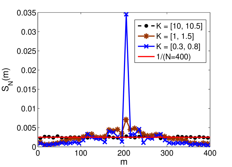
The distribution of the position of the maximum intensity in the position representation is shown in Fig. 8(a), where one can see a transition to the uniform distribution along with the transition to classical chaos. As has been discussed above, in the context of the quantity $S_{N}(m)$, the probability that the final record, which is also the maximum, lasts for time $m$ is independent of $m$ for both i.i.d. and delta correlated variables. Thus the uniform distribution of the maximum intensity is consistent with this.

The sharp peak at the center for small $K$ (here $K=0.3$) deserves further analysis. In Srivastava et al. (2013), it has been pointed out that for small $K$, when there are many narrow classical resonances, a large fraction of eigenfunctions are localized on separatrices and have maximum intensity at or very close to $q=1/2$, although this is an unstable fixed point (zero momentum). For example, with $N=400$, $K=0.1$ and $0.3$, about $75\%$ and $50\%$ of eigenstates are peaked at $q=1/2$. This is because at the prominent $0/1$ resonance corresponding to the fixed points, $q=1/2$ is near the turning point of orbits on which the eigenstates are localized.

As $K$ increases there are more prominent resonances and turning points move away from $q=1/2$. Eigenstates localize in the resonance interiors, thereby the maximum intensity shifts away from $q=1/2$. This was the qualitative picture put forward in Srivastava et al. (2013) as leading to the uniform distribution for maximum intensity for large $K$. This qualitative explanation is also well supported by the distribution of the position of the minimum in the position representation. As we expect and indeed observe that most of the states have their minimum around stable fixed point, i.e. $q=0$ (see Fig. 8(b)). The transition in classical behavior from integrable ($K=0$), to mixed phase space where islands of stability coexist within the stochastic sea (intermediate $K$), to fully-developed chaos is thus well captured by the quantity $S_{N}(m)$, the distribution of the position of extreme intensities.

(a) upper record

(b) lower record

Figure 8: The distribution of the position of the last record set, which is also the maximum in case of upper record and minimum in case of lower record, for eigenfunctions of the standard map with $N=400$ and for various values of $K$. In Fig. 8(b), inset shows a zoomed in view to clearly see the features of $S_{N}(m)$ as function of $m$ for various $K$ values.

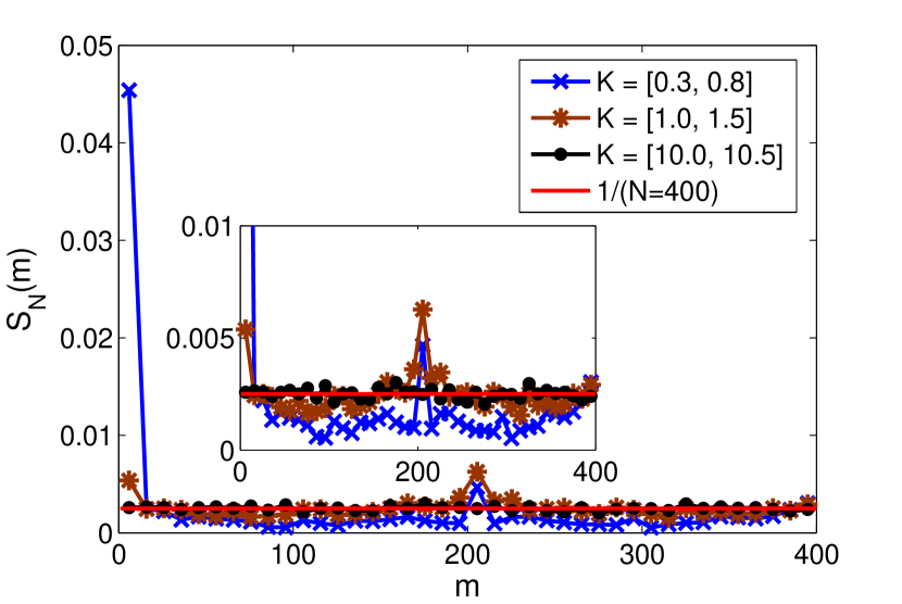
It has been shown above that for random $N$-dimensional states the number of intensity records increases as in the i.i.d. case, namely as $\sim\log N+\gamma$ both upper and lower records. While we expect to see this for the quantum standard map eigenfunctions in the strongly chaotic, large $K$ regime, the mixed and near-integrable regimes show a marked departure that were discussed in Srivastava et al. (2013) for the case of upper records. The correlations present for small $K$ lead to results that are similar to those for the random walks, or the classical standard map and results in records increasing as a power-law with $N$. For example it was found that it is almost a pure power-law with exponent $0.5$ at the critical value $K=0.98$, exactly like that of random walks.

4 Summary

We have shown that time evolution of records for squared deviation of momentum of the classical standard map follows a power law. In a heuristic manner, it has been argued why in the hard chaos regime this is the same as the results for discrete random walks with jump distribution being i.i.d. random variables. Hence, any deviation from such a result accounts for the correlation present in dynamical system, and is clearly borne out in the numerical simulations. The deviation for the large $K$ regime is due to the presence of accelerator modes, and result in records that maybe relevant for correlated Levy walks. Even, in the mixed phase regime the higher period accelerator modes seem to affect the records.

We have reviewed the results on upper records of intensities of correlated random vectors and derived new ones for lower records. Apart from deriving the average record, it has been shown that the probability that a record appears at an index $j$ is a Bernoulli process, which is the same as for i.i.d. variables. The quantum standard map is a good test bed and has increasingly complex spectrum with the system parameter $K$. For a quantum system with random high-lying states, records’ statistics for random vectors applies. Also the study of the position of the last record set in the case of the standard map, parametrized by $K$ suggests that beyond a certain value of $K$, the eigenvectors do become like random vectors insofar as the records of intensities is concerned. This is also consistent with finding where the number of records vs $N$ goes through a transition from a power law to logarithmic, as $K$ increases.

We have essentially begun studying classical and quantum dynamical systems using novel measures related to the theory of extremes and records, and hope to have shown that this is fruitful and interesting enough to pursue further.

References

- Arnold et al. (1998) Arnold, B. C., Balakrishnan, N., Nagaraja, H. N., 1998. Records. John Wiley & Sons, New York.
- Bäcker (2003) Bäcker, A., 2003. Numerical Aspects of Eigenvalue and Eigenfunction Computations for Chaotic Quantum Systems. Vol. 618 of Lect. Notes in Phys. Springer-Verlag, Berlin.
-
Bai et al. (1998)
Bai, Z.-D., Hwang, H.-K., Liang, W.-Q., 1998. Normal approximations of the
number of records in geometrically distributed random variables. Random
Structures and Algorithms 13 (3-4), 319.
URL http://dx.doi.org/10.1002/(SICI)1098-2418(199810/12)13:3/4<319::AID-RSA7>3.0.CO;2-Y -
Bazant (2000)
Bazant, M. Z., Aug 2000. Largest cluster in subcritical percolation. Phys. Rev.
E 62, 1660–1669.
URL http://link.aps.org/doi/10.1103/PhysRevE.62.1660 -
Berry et al. (1979)
Berry, M. V., Balazs, N. L., Tabor, M., Voros, A., 1979. Quantum maps. Ann.
Phys. (NY) 122, 26–63.
URL http://dx.doi.org/10.1016/0003-4916(79)90296-3 -
Biswas and Jain (1990)
Biswas, D., Jain, S. R., Sep 1990. Quantum description of a pseudointegrable
system: The /3-rhombus billiard. Phys. Rev. A 42, 3170–3185.
URL http://link.aps.org/doi/10.1103/PhysRevA.42.3170 - Bohigas et al. (1984) Bohigas, O., Giannoni, M.-J., Schmit, C., 1984. Characterization of Chaotic Quantum Spectra and Universality of Level Fluctuation Laws. Phys. Rev. Lett. 52, 1.
- Brody et al. (1981) Brody, T. A., Flores, J., French, J. B., Mello, P. A., Pandey, A., Wong, S. S. M., 1981. Random-matrix physics: Spectrum and strength fluctuations. Rev. Mod. Phys. 53, 385 – 479.
- Casati and Ford (1979) Casati, G., Ford, J. (Eds.), 1979. Stochastic Behavior in Classical and Quantum Hamiltonian Systems. Vol. 93 of Lect. Notes in Phys. Springer-Verlag, Berlin.
Chang and Shi (1986)
Chang, S.-J., Shi, K.-J., Jul 1986. Evolution and exact eigenstates of a
resonant quantum system. Phys. Rev. A 34, 7–22.
URL http://link.aps.org/doi/10.1103/PhysRevA.34.7 - Chirikov (1979) Chirikov, B. V., may 1979. A universal instability of many-dimensional oscillator systems. Phys. Rep. 52, 263–379.
- Gembris et al. (2002) Gembris, D., Taylor, J. G., Suter, D., 2002. Sports statistics: Trends and random fluctuations in athletics. Nature 417, 506.
- Glick (1978) Glick, N., 1978. Breaking records and breaking boards. American Mathematical Monthly 85, 2.
Godrèche et al. (2014)
Godrèche, C., Majumdar, S. N., Schehr, G., 2014. Universal statistics of
longest lasting records of random walks and lévy flights. Journal of Physics
A: Mathematical and Theoretical 47 (25), 255001.
URL http://stacks.iop.org/1751-8121/47/i=25/a=255001 - Haake (1991) Haake, F., 1991. Quantum Signatures of Chaos. Springer-Verlag, New York.
- Heller (1984) Heller, E. J., 1984. Bound-state eigenfunctions of classically chaotic hamiltonian systems: Scars of periodic orbits. Phys. Rev. Lett. 53, 1515.
- Izrailev (1999) Izrailev, F., 1999. Simple models of quantum chaos: Spectrum and eigenfunctions. Phys. Rep. 196, 299–392.
Kudrolli et al. (1995)
Kudrolli, A., Kidambi, V., Sridhar, S., Jul 1995. Experimental studies of chaos
and localization in quantum wave functions. Phys. Rev. Lett. 75, 822–825.
URL http://link.aps.org/doi/10.1103/PhysRevLett.75.822 -
Lakshminarayan (2009)
Lakshminarayan, A., 2009. SERC School-2009, Delhi University: Lecture Notes.
www.physics.iitm.ac.in/ãrul/serc/serc1.html.
URL www.physics.iitm.ac.in/ãrul/serc/serc1.html - Lakshminarayan et al. (2008) Lakshminarayan, A., Tomsovic, S., Bohigas, O., Majumdar, S. N., 2008. Extreme Statistics of Complex Random and Quantum Chaotic States. Phys. Rev. Lett. 100, 044103.
Laurent et al. (2007)
Laurent, D., Legrand, O., Sebbah, P., Vanneste, C., Mortessagne, F., Dec 2007.
Localized modes in a finite-size open disordered microwave cavity. Phys. Rev.
Lett. 99, 253902.
URL http://link.aps.org/doi/10.1103/PhysRevLett.99.253902 -
MacKay et al. (1984)
MacKay, R. S., Meiss, J. D., Percival, I. C., Feb 1984. Stochasticity and
transport in hamiltonian systems. Phys. Rev. Lett. 52, 697–700.
URL http://link.aps.org/doi/10.1103/PhysRevLett.52.697 -
Majumdar et al. (2012)
Majumdar, S. N., Schehr, G., Wergen, G., 2012. Record statistics and
persistence for a random walk with a drift. Journal of Physics A:
Mathematical and Theoretical 45 (35), 355002.
URL http://stacks.iop.org/1751-8121/45/i=35/a=355002 - Majumdar and Ziff (2008) Majumdar, S. N., Ziff, R. M., 2008. Universal Record Statistics of Random Walks and Lévy Flights. Phys. Rev. Lett. 101, 050601.
Manos and Robnik (2014)
Manos, T., Robnik, M., feb 2014. Survey on the role of accelerator modes for
anomalous diffusion: The case of the standard map. Phys. Rev. E 89 (2),
022905.
URL http://link.aps.org/doi/10.1103/PhysRevE.89.022905 -
McDonald and Kaufman (1979)
McDonald, S. W., Kaufman, A. N., Apr 1979. Spectrum and eigenfunctions for a
hamiltonian with stochastic trajectories. Phys. Rev. Lett. 42, 1189–1191.
URL http://link.aps.org/doi/10.1103/PhysRevLett.42.1189 - Mehta (2004) Mehta, M. L., 2004. Random Matrices. Elsevier Academic Press, London.
Moore et al. (1995)
Moore, F., Robinson, J., Bharucha, C., Sundaram, B., Raizen, M., Dec 1995. Atom
optics realization of the quantum -kicked rotor. Phys. Rev. Lett.
75, 4598–4601.
URL http://link.aps.org/doi/10.1103/PhysRevLett.75.4598 - Nevzorov (1987) Nevzorov, V. B., 1987. Records. Theory of Probability and its Applications 32, 201.
Oliveira et al. (2005)
Oliveira, L. P., Jensen, H. J., Nicodemi, M., Sibani, P., Mar 2005. Record
dynamics and the observed temperature plateau in the magnetic creep-rate of
type-ii superconductors. Phys. Rev. B 71, 104526.
URL http://link.aps.org/doi/10.1103/PhysRevB.71.104526 -
Redner and Petersen (2006)
Redner, S., Petersen, M. R., Dec 2006. Role of global warming on the statistics
of record-breaking temperatures. Phys. Rev. E 74, 061114.
URL http://link.aps.org/doi/10.1103/PhysRevE.74.061114 - Rényi (1962) Rényi, A., 1962. Théorie des éléments saillants d’une suite d’observations, Selected Papers of Alfred Renyi. Vol. 2. Academic Press, New York.
Sabhapandit (2011)
Sabhapandit, S., 2011. Record statistics of continuous time random walk. Eur.
Phys. Lett. 94 (2), 20003.
URL http://stacks.iop.org/0295-5075/94/i=2/a=20003 -
Saraceno (1990)
Saraceno, M., 1990. Classical structures in the quantized baker transformation.
Ann. Phys. (NY) 199 (1), 37 – 60.
URL http://www.sciencedirect.com/science/article/pii/000349169090367W - Schehr and Majumdar (2013) Schehr, G., Majumdar, S. N., May 2013. Exact record and order statistics of random walks via first-passage ideas. World Scientific.
Schmittmann and Zia (1999)
Schmittmann, B., Zia, R. K. P., dec 1999. “weather” records: Musings on
cold days after a long hot indian summer. Am. J. Phys. 67 (12), 1269–1276.
URL http://scitation.aip.org/content/aapt/journal/ajp/67/12/10.1119/1.19114 -
Srivastava et al. (2013)
Srivastava, S. C. L., Lakshminarayan, A., Jain, S. R., 2013. Record statistics
in random vectors and quantum chaos. Eur. Phys. Lett. 101, 10003.
URL http://arxiv.org/abs/1205.0698 -
Tomsovic and Lakshminarayan (2007)
Tomsovic, S., Lakshminarayan, A., Sep 2007. Fluctuations of finite-time
stability exponents in the standard map and the detection of small islands.
Phys. Rev. E 76, 036207.
URL http://link.aps.org/doi/10.1103/PhysRevE.76.036207 - Vogel et al. (2001) Vogel, R. M., Zafirakou-Koulouris, A., Matalas, N. C., 2001. Frequency of record-breaking floods in the United States. Water Res. Research 37, 1723.
Wergen et al. (2011)
Wergen, G., Bogner, M., Krug, J., May 2011. Record statistics for biased random
walks, with an application to financial data. Phys. Rev. E 83, 051109.
URL http://link.aps.org/doi/10.1103/PhysRevE.83.051109